Noninvasive Assessment of Existing Concrete

Transcription

1 Noninvasive Assessment of Existing Concrete FINAL REPORT February 2, 2016 By Piervincenzo Rizzo University of Pittsburgh COMMONWEALTH OF PENNSYLVANIA DEPARTMENT OF TRANSPORTATION CONTRACT # WORK ORDER # PIT 008

2 Technical Report Documentation Page 1. Report No. FHWA-PA PIT WO Government Accession No. 3. Recipient s Catalog No. 4. Title and Subtitle Noninvasive Assessment of Existing Concrete 7. Author(s) Piervincenzo Rizzo, Ph.D. University of Pittsburgh, Dept. of Civil & Environmental Engineering 3700 O'Hara Street, 729 Benedum Hall Pittsburgh, PA USA pir3@pitt.edu, Phone: Performing Organization Name and Address University of Pittsburgh, 123 University Place Pittsburgh, PA, Report Date 02/02/ Performing Organization Code 8. Performing Organization Report No. 10. Work Unit No. (TRAIS) 11. Contract or Grant No , PIT WO Sponsoring Agency Name and Address The Pennsylvania Department of Transportation Bureau of Planning and Research Commonwealth Keystone Building 400 North Street, 6 th Floor Harrisburg, PA Type of Report and Period Covered Final Report 2/03/2015 2/02/ Sponsoring Agency Code 15. Supplementary Notes Technical Advisor Ronald D. Schreckengost, Jr., P.E. PA Department of Transportation District Oakland Avenue, PO Box 429 Indiana PA ROSCHRECKE@pa.gov, Phone: Abstract The nondestructive evaluation (NDE) of concrete has been a long-standing challenge. In the last three decades, many NDE methods have been proposed, and some of them resulted in commercial products. The most common method is probably the one based on the measurement of the velocity of bulk ultrasonic waves propagating through concrete. The measurement helps to assess the strength of concrete or to monitor the curing of fresh concrete. Another popular commercial system is the Schmidt hammer that consists of a springdriven steel hammer that hits the specimen with a defined energy. Part of the impact energy is absorbed by the plastic deformation of the specimen, and the remaining impact energy is rebounded. The rebound distance depends on the hardness of the specimen and the conditions of the surface. As these methods are not universally accepted, much research is still ongoing on the NDE of concrete. In this report, we preset an NDE method based on the propagation of highly nonlinear solitary waves (HNSWs) along a 1-D chain of spherical particles in contact with the concrete to be tested. With respect to ultrasonic-based NDE, the proposed approach: 1) exploits the propagation of waves confined within the grains; 2) employs a cost-effective transducer; 3) measures different waves parameters (time of flight, speed, and amplitude of one or two pulses); 4) does not require any knowledge of the sample thickness; 5) does not require an access to the sample s back-wall. Moreover, the method differs from the Schmidt hammer because it can be applied also onto fresh concrete, multiple HNSWs features can be exploited, and it does not induce plastic deformation. In this project, the propagation of HNSWs is used to measure the strength of cured concrete under concrete s control mix design and under excessive water/cement (w/c) ratio. The objective was the assessment of the modulus of hardened concrete to predict the compressive strength of bridge concrete decks, or other concrete structures. In the work presented here many HNSW-based transducer were used to test concrete cylinders cast with well controlled w/c ratios and short beams cast with a certain w/c ratio but corrupted with excessive water. The latter mimicked rainfall prior, during, and after construction. We monitor the characteristics of the waves reflected from the transducer/concrete interface in terms of their amplitude and time-of-flight (TOF). The latter denotes the transit time at a given sensor bead in the granular crystal between the incident and the reflected waves. When a single HNSW interacts with a "soft" neighboring medium, secondary reflected solitary waves (SSW) form in the granular crystal, in addition to the primary reflected solitary waves (PSW). We observed that the waves propagating within the transducer are affected by the amount of water present in the mix design. Future studies shall expand the research by including more samples and by conducting field tests in existing bridges. 17. Key Words Nondestructive evaluation, highly nonlinear solitary waves, concrete modulus, water-to-cement ratio. 19. Security Classif. (of this report) 20. Security Classif. (of this page) 18. Distribution Statement No restrictions. This document is available from the National Technical Information Service, Springfield, VA No. of Pages 22. Price Unclassified Unclassified 117 N/A Form DOT F (8-72) Reproduction of completed page authorized

3 STATEMENT OF CREDIT This work was sponsored by the Pennsylvania Department of Transportation and the U.S. Department of Transportation, Federal Highway Administration. DISCLAIMER The contents of this report reflect the views of the author(s) who is(are) responsible for the facts and the accuracy of the data presented herein. The contents do not necessarily reflect the official views or policies of the US Department of Transportation, Federal Highway Administration, or the Commonwealth of Pennsylvania at the time of publication. This report does not constitute a standard, specification or regulation. iii

4 TABLE OF CONTENTS STATEMENT OF CREDIT DISCLAIMER TABLE OF CONTENTS LIST OF FIGURES LIST OF TABLES iii iii iv vi xiv CHAPTER 1: INTRODUCTION Problem Statement and Motivation Scope of Work Report Outline 4 CHAPTER 2: LITERATURE REVIEW Theoretical Background HNSW Transducer Cement: Experimental Setup Cement: Numerical Setup and Results Cement: Experimental Results Concrete: Experimental Setup Concrete: Results Conclusions 23 CHAPTER 3: LABORATORY SAMPLES Mix Design of the Concrete Cylinders Mix Design of the Short Concrete Beams 30 CHAPTER 4: DESIGN AND ASSEMBLY OF THE NONDESTRUCTIVE EVALUATION METHODS Highly Nonlinear Solitary Waves: Experimental Setup Ultrasonic Pulse Velocity (UPV) Method: Experimental Setup Repeatability Tests Materials Testing Numerical Model Concrete Testing: Setup Concrete Testing: Results Summary 71 CHAPTER 5: NONDESTRUCTIVE AND ASTM TESTING (28 DAYS TESTS) 74 iv

5 5.1. Concrete Cylinders and Test Protocol Results of the M-Transducers Results of the P-Transducers Young s Modulus Computation Destructive Testing Using ASTM C39 and C UPV Testing HNSW-based Transducers Comparison from All Methods Short Beams with Standing Water During Concreting HNSW Results Results of UPV Test Conclusions 91 CHAPTER 6: NONDESTRUCTIVE AND ASTM TESTING (122 DAYS TESTS) Results of the HNSW-based Transducers Results of M-Transducers Results of P-transducers Estimation of the Modulus of Elasticity of the Cylinders Moduli of Elasticity Measured by M-transducers Modulus of Elasticity Measured using P-transducers Results of the UPV Test Results of the ASTM C Comparison of the Methods for Estimating the Moduli of Elasticity of the Cylinders Testing Short Beams with Standing Water During Concreting NDE Results Result of HNSW-based Transducers Result of the UPV Tests Summary 112 CHAPTER 7: SUMMARY AND FUTURE RESEARCH 113 REFERENCE 115 v

6 LIST OF FIGURES Fig. 1.1 (a) Through-transmission. Two L transducers or S transducers are used to transmit and receive bulk waves. Wave speed and amplitude are measured. Drawbacks: 1) in order to exploit both modes (S and L) four transducers are necessary; 2) access to the back-wall is necessary, which is not always possible; 3) to accurately measure the speed the exact distance between the transducers is necessary; 4) to avoid any mislead assessment of the amplitude the contact conditions between the transducers and the concrete surface must be kept constant. (b) Pulse-echo configuration. One L- or S-transducer is used in the dual-mode, i.e. as both transmitter and receiver. A buffer material is interposed between the transducer and the concrete. As the wave speed in the buffer material is constant irrespective of the concrete age, only one wave parameter (the amplitude) can be exploited unless two transducers (one S- and one L-) are used. Fig. 1.2 (Left column): photo of concrete bridge deterioration; photos on the left are from the authors. (Right column): excessive water bleed during construction; photos provided by Penn DOT Fig. 1.3 Scheme of the NDE method based on the propagation of HNSWs Fig. 2.1 (a) Photo of the HNSW transducer for the remote non-contact generation of HNSWs. A mechanical grip is used to hold the transducer during the experiments presented here. (b) Schematic diagram of the HNSW transducer. Dimensions are in mm. (c) Photo of a typical instrumented particle devised for the detection of the propagating solitary waves (Ni et al. 2012) Fig. 2.2 Photo of the experimental setup. The HNSW transducer is positioned on the gypsum cement sample, and a DC power supply is connected to the electromagnet inside the HNSW transducer. Two instrumented sensors at the 11 th and 16 th particle positions in the HNSW transducer measure force profiles of reflected waves, which are digitized and stored by an oscilloscope Fig. 2.3 FEM simulation of HNSW interaction with gypsum cement samples in various elastic condition. All signals represent propagating waves through the 11th bead in the chain. To ease visualization, the signals are shifted by 10 N in the vertical axis. The time of flight (TOF) values of HNSWs are extracted by measuring the time elapsed between the incident (the leftmost impulses) and the first reflected wave (subsequent impulses) Fig. 2.4 Numerical results showing time of flight and propagating speed of HNSWs. Solid lines represent fitted curves based on polynomial least square method. (a) Time of flight of the primary (circular blue dots) and secondary (square red dots) reflected solitary waves as a function of the cement s elastic modulus. (b) Velocity of incident (crossed green dots) and primary reflected (circular blue dots) solitary waves Fig. 2.5 Numerical results showing amplitude ratios of the primary (circular blue dots) and secondary (square red dots) reflected solitary waves as a function of the cement s elastic modulus. Solid lines are based on polynomial curve-fitting using least square method Fig. 2.6 Experimental results of HNSW interaction with gypsum cement samples in various cement age. The force profiles are measured from the 11th bead in the HNSW transducer Fig. 2.7 Experimental results showing time of flight and propagating speed of HNSWs. The vertical error bars represent standard deviations obtained from five signal measurements, and the solid lines denote the fitted curves based on discrete measurement data. (a) TOF of the primary (circular blue dots) and secondary (square red dots) waves as a function of cement age. (b) Velocity of the incident (crossed green dots), primary reflected (circular blue dots), and secondary reflected (square red dots) HNSWs as a function of cement age vi

7 Fig. 2.8 Experimental measurements of amplitude ratios of the primary (circular blue dots) and secondary (square red dots) reflected solitary waves as a function of cement age Fig. 2.9 Measurements of cement compressive strength as a function of the cement age. (a) 15 Compressive strength superimposed to the TOF variation of the PSWs as recorded by the 11th bead. (b) Compressive strength superimposed to the amplitude ratio of the PSWs as measured by 11th bead. For the sake of clarity the error bars are removed from the plots of the HNSW-based features Fig Young s modulus of 50-mm cubic cement samples as a function of cement age. The 16 blue dots represent measurement results based on a series of compression tests, while the solid blue line represents a fitted curve Fig Comparison of experimental and numerical data for the time of flight (TOF) as a 17 function of the cement s elastic modulus. Numerical results of TOFs for the primary and secondary reflected waves are denoted by solid blue and red curves, while experimental measurements of PSW s and SSW s TOF values are represented by blue and red dots, respectively Fig Photo of the experimental setup. Top left: close-up view of the switch circuit 18 Fig Force profile of the HNSWs waveforms recorded at different ages of concrete. 19 Measurements taken at the (a) 11th bead and (b) 16th bead Fig TOF of the PSW (TOFP) and SSW (TOFS) measured from the (a) 11th and 20 (b) 16th bead in the HNSW transducer and penetration resistance as a function of time Fig (a) Experimental results of wave speed of incident HNSW and PSW. (b) The ratio of the 21 wave speed of PSW to that of incident HNSW Fig The value of amplitude ratio as a function of time Fig. 3.1 Scheme of the cylindrical samples cast in this project 24 Fig. 3.2 Loading raw materials for mixing 28 Fig. 3.3 Butter batch unloading 28 Fig. 3.4 Air content measurement 28 Fig. 3.5 Slump test 28 Fig. 3.6 Batch #1 mixture consistency 29 Fig. 3.7 Finishing cylinders 29 Fig. 3.8 Burlap and plastic sheet cover 29 Fig. 3.9 Scheme of the concrete beams. (a) condition 1: 0.5 in excessive water at the bottom of the 30 beam, to mimic standing water on the formwork before concreting. (b) condition 2: 0.25 in excessive water at the bottom of the beam, to mimic standing water on the formwork before concreting. (c) condition 3: 0.10 in excessive water at the top of the beam, to mimic rain during concreting. (d) condition 4: 0.15 in excessive water at the top of the beam, to mimic rain during concreting Fig Batch #1 mixture consistency 34 Fig Air content measurement 34 Fig Slump test 35 Fig Pouring standing water in bottom of prepared beam molds (condition 1) 35 Fig Verifying standing water depth 35 vii

8 Fig Placing concrete into beam mold with standing water (condition 1) 35 Fig Internal vibration of beam mold (condition 1) 36 Fig Beam mold surface after internal vibration causes standing water to rise (condition 1) 36 Fig Finishing surface of beam mold (condition 1) 36 Fig Concrete placement before any surface water applied and finished (condition 3) 36 Fig First application of surface water (condition 3) 37 Fig Beam surface after first application of surface water (condition 3) 37 Fig Second application of surface water applied to beam surface after finishing (condition 3) 37 Fig Finishing beam surface after second application of water (condition 3) 37 Fig Rodding beam surface before final application of water (condition 3) 38 Fig Third and final application of surface water (condition 3) 38 Fig Beam surface after third application of water (condition 3) 38 Fig Finishing beam surface (condition 3) 38 Fig Concrete placement into beam mold with standing water (condition 2) 39 Fig Standing water from bottom of beam mold (condition 2) 39 Fig Internal vibration of beam mold (condition 2) 39 Fig Finishing beam top surface (condition 2) 39 Fig Concrete placement before condition 4 surface water applied 40 Fig First application of surface water (condition 4) 40 Fig Top surface of beam mold after first application of surface water (condition 4) 40 Fig Internal vibration of beam mold (condition 4) 40 Fig Rodding top surface of beam mold (condition 4) 41 Fig Top surface of beam mold after rodding (condition 4) 41 Fig Second application of surface water (condition 4) 41 Fig Top surface of beam mold after second application of surface water (condition 4) 41 Fig Finishing top surface of beam mold after second application of surface water (condition 42 4) Fig Rodding of beam surface after first surface finishing (condition 4) 42 Fig Third and final application of surface water (condition 4) 42 Fig Finishing beam surface (condition 4) 42 Fig Casting compression cylinders from same batch as beams (condition 4) 43 Fig Loading raw material for mixing 43 Fig Air content measurement 43 Fig Batch #1 mixture consistency 44 Fig Slump test 44 Fig Beam mold preparation with standing water (condition 1) 44 Fig Verifying standing water depth (condition 1) 44 Fig Evenly placing concrete in beam mold with standing water (condition 1) 45 Fig Top surface after concrete placement into beam mold with standing water (condition 1) 45 viii

9 Fig Internal vibration of beam mold (condition 1) 45 Fig Finishing surface of beam mold (condition 1) 45 Fig Finished surface of beam mold (condition 1) 46 Fig Concrete placement before top surface water application (condition 3) 46 Fig Surface water application (condition 3) 46 Fig Top surface after first application of surface water (condition 3) 46 Fig Internal vibration of beam mold (condition 3) 47 Fig Striking off top surface (condition 3) 47 Fig Top surface before first rodding application (condition 3) 47 Fig First rodding application (condition 3) 47 Fig Top surface after rodding (condition 3) 48 Fig Second application of surface water (condition 3) 48 Fig Finishing top surface after second application of surface water (condition 3) 48 Fig Top surface after second application of rodding (condition 3) 48 Fig Top surface after third and final application of surface water (condition 3) 49 Fig Finished top surface (condition 3) 49 Fig Concrete placement into beam mold with standing water (condition 2) 50 Fig Internal vibration of beam mold (condition 2) 50 Fig Finished top surface (condition 2) 50 Fig Concrete placement in beam mold before surface water application (condition 4) 50 Fig First application of surface water (condition 4) 51 Fig Internal vibration of beam mold (condition 4) 51 Fig Striking off top surface (condition 4) 51 Fig First application of rodding (condition 4) 51 Fig Second application of surface water (condition 4) 52 Fig Finishing top surface (condition 4) 52 Fig Second and final application of rodding (condition 4) 52 Fig Third and final application of surface water (condition 4 52 Fig Finished top surface (condition 4 53 Fig. 4.1 (a) Schematic of the M-transducers; (b) schematic of the P-transducers; (c) The schematic view of parts of the PZT sensor-rods Fig. 4.2 The hardware: (a) the control circuit. EM1 to EM4 represents four electromagnets 56 mounted on sensor 1 to sensor 4 respectively. Switches 1 to 4 are digital switches, and if one of them is set as 1, the switch will be turned on. (b) Left to right: photos of the PXI utilized in the experiments, the DC Power supply, used to provide electromagnet with direct voltage, and the switch circuit with a MOSFET and two terminal blocks Fig. 4.3 Photo of the M-transducer in air, water, on soft polyurethane, hard polyurethane and 57 stainless steel Fig. 4.4 Left column: averaged time waveforms when testing in air (a), water (b), soft ix

10 polyurethane (c), hard polyurethane (d), and stainless steel (e). Right column: corresponding voltage integral. Each figure has four curves that are associated, from bottom to top, with the sensor 1 to 4, respectively Fig. 4.5 Time of flight associated with the (a) primary reflected wave (TOF PSW ) and (b) the secondary reflected solitary wave (TOF SSW ) as a function of the five different media in contact with the solitary wave transducers Fig. 4.6 Numerical results. Force profile of the HNSWs propagating through the 9th particle of a chain of steel spheres in contact with the five different media considered in the experiments. Fig. 4.7 Numerical results. TOF PSW as a function of the Young's modulus and Poisson's ratio of the material in contact with the chain of particles Fig. 4.8 Numerical results. Ratio PSW/ISW as a function of the Young's modulus and Poisson's 64 ratio of the material in contact with the chain of particles Fig. 4.9 Numerical results. Ratio SSW/ISW as a function of the Young's modulus and Poisson's 64 ratio of the material in contact with the chain of particles Fig Experimental setup 66 Fig The experimental setup and schematic of the UPV test 66 Fig Example of transmitted (blue solid line) and received (dashed red line) signals in the 67 UPV testing of the concrete slabs. The time interval between the first peak of both lines was considered Fig The output voltage integral waveforms of the four sensors, of which the top curve is the 68 signal obtained by sensor 4 and the bottom curve is obtained by sensor 1 Fig Averaged value of the 100 measurements taken by the four transducers at four different 68 surface location of the eight slabs. (a) Feature of the TOF PSW ; (b) feature of the TOF SSW. The small vertical bars represent the standard deviation of the experimental data Fig The surface of slab (a) 1, (b) 3 and (c) 4. There are many voids on the surface of slab 71 1and 3, on the contrary, slab 4 has a much smoother surface with fewer voids Fig The average estimated static modulus of elasticity and the corresponding standard 72 deviations of the four different methods Fig. 5.1 Typical (a) M-transducers set-up, (b) P-transducers set-up 75 Fig. 5.2 Fig. 5.2 UPV testing: (Left) along and (Right) perpendicular the axis of the cylinder Fig. 5.3 (a) Voltage waveform of M1 for the cylinders with different w/c; (b) Integrated voltage 76 waveform of M1 for the cylinders with different w/c; (c) A close-up view of the voltage waveform of M1 for each batch; (d) A close-up view of the integrated voltage waveform of M1 for each batch Fig. 5.4 TOFs and associated standard deviations obtained from the three different batches 77 Fig. 5.5 (a) Time waveform recorded by P1 for the cylinders with different w/c; (b) A close-up 77 view of the time waveform and the TOF of each w/c ratio Fig. 5.6 TOF and associated standard deviation values measured vs w/c ratio 78 Fig. 5.7 The modulus of elasticity and associated standard deviations measured in accordance 79 with the ASTM C496 Fig. 5.8 A typical waveform recorded from UPV test 80 Fig. 5.9 (a) The measured UPV wave velocities of the cylinders. (b) The estimated modulus of 81 elasticity of cylinders with different w/c from UPV test x

11 Fig Numerical model. (a) TOF as a function of the dynamic modulus of elasticity and the Poisson s ratio; (b) TOF as a function of the modulus of elasticity when ν=0.20 Fig The Average modulus of elasticity of various studied methods 83 Fig (a) condition 1: 0.5 in excessive water at the bottom of the beam, (b) condition 2: 0.25 in excessive water at the bottom of the beam, (c) condition 3: 0.10 in excessive water at the top of the beam, (d) condition 4: 0.15 in excessive water at the top of the beam Fig (a) Placing M-transducers on the beams; (b) placing P-transducers on the beams 85 Fig (a) UPV test set-up; (b) A typical waveform recorded by UPV test for the beams 90 Fig (a) Pulse velocity of the ultrasonic pulse; (b) modulus of elasticity of the beams measured by the UPV test Fig. 6.1 Results of M-transducers: (a) voltage waveform of M1, (b) comparison of the voltage waveforms of M1, (c) integrated voltage waveform of M1, (d) comparison of the integrated voltage waveforms of M1 for the cylinders with different w/c Fig. 6.2 TOFs and associated standard deviations of the cylinders measured by the M-transducers 94 Fig. 6.3 (a) Time waveform recorded by P1 for the cylinders with different w/c; (b) A close-up view of the time waveform and the TOF of each w/c Fig. 6.4 TOF and associated standard deviation values obtained from the time waveforms of the 96 considered batches measured by the P-transducers Fig. 6.5 The predicted modulus of elasticity of each cylinder obtained by the M-transducer 97 Fig. 6.6 The predicted modulus of elasticity of each cylinder obtained by the P-transducers 98 Fig. 6.7 UPV test results: (a) Pulse velocity and (b) modulus of elasticity of the Cylinders 99 Fig. 6.8 Modulus of elasticity determined using four different methods: (a) Tests conducted days after curing on July/07/2015; (b) Tests conducted 122 days on October/06/2015 Fig. 6.9 (a) condition 1: 0.5 in excessive water at the bottom of the beam, (b) condition 2: 0.25 in 103 excessive water at the bottom of the beam, (c) condition 3: 0.10 in excessive water at the top of the beam, (d) condition 4: 0.15 in excessive water at the top of the beam Fig Modulus of elasticity measure at bottom and top surface using (a) M-transducers and (b) 109 P-transducers Fig (a) Pulse velocity of the ultrasonic pulse; (b) modulus of elasticity of the beams 111 measured by the UPV test Fig Comparison of the modulus of elasticity of the beams measure by different methods xi

12 LIST OF TABLES Table 2.1 Mechanical properties of materials used in the experiments 9 Table 2.2 Summary of the PCC mixture design used for the test 17 Table 3.1 Design of the Concrete Mixture 24 Table 3.2 Material properties 26 Table 3.3 Batch #1 Mixture Design 26 Table 3.4 Liquid Admixture Dosage for Batch #1 26 Table 3.5 Batch #2 Mixture Design 26 Table 3.6 Liquid Admixture Dosage for Batch #2 27 Table 3.7 Batch #3 Mixture Design 27 Table 3.8 Liquid Admixture Dosage for Batch #3 27 Table 3.9 Different conditions created in the short beams in order to mimic rain prior and after concreting Table 3.10 Labels of the short beams Table 4.1 Properties of the polyurethane and stainless steel. The values of polyurethane are from Biomechanical Test Material Sawbones. The parameters of stainless steel are from ASM material data sheet Table 4.2 Calibration coefficient of the four magnetostrictive sensors. The coefficients are used to convert the voltage amplitude associated with the propagation of the solitary waves into Newton Table 4.3 Average TOFPSW and TOFSSW and corresponding standard deviations measured when testing the five different media Table 4.4 Experimental and numerical TOFPSW and their difference 65 Table 4.5 Parameters obtained from ASTM C469 and ASTM C39 65 Table 4.6 Size and weight of tested concrete slab samples 65 Table 4.7 Eastimating Young's Modulus of Concrete slab samples using HNSW-based sensors, Ultrasonic Testing, and Destructive testing Table 4.8 UPV test. Velocity of the longitudinal bulk wave and predicted dynamic and static modulus of elasticity Table 4.9 Concrete tests. Estimated static modulus of elasticity of the test samples using two destructive and two nondestructive methods Table 5.1 The detailed information of the concrete cylinders 74 Table 5.2 The TOF and standard deviation values of the M-transducers 76 Table 5.3 The TOF and standard deviation values measured by P-transducers for different batches 78 Table 5.4 Concrete parameters obtained through ASTM C39 and ASTM C Table 5.5 The modulus of elasticity of each cylinder obtained by the UPV test 80 Table 5.6 The estimated modulus of elasticity of each cylinder obtained by the M-transducers 82 Table 5.7 The predicted modulus of elasticity of each cylinder through P-transducers 82 xii

13 Table 5.8 The modulus of elasticity estimated via various methods 83 Table 5.9 Different considered conditions and notations of the beams 85 Table 5.10 The TOF and modulus of elasticity of the beams in which condition 1 was imposed 86 Table 5.11 The TOF and modulus of elasticity of the beams in which condition 2 was imposed 87 Table 5.12 The TOF and modulus of elasticity of the beams in which condition 3 was imposed 88 Table 5.13 The TOF and modulus of elasticity of the beams in which condition 4 was imposed 89 Table 5.14 The modulus of elasticity of the beams in which different conditions measured by UPV test Table 5.15 Summary of the experimental results associated with the samples tested after 28 days. The cylinders were tested only from one side. The short beams were tested through the thickness with the UPV technique Table 6.1 Properties of the materials used to fabricate the cylinders 93 Table 6.2 Properties and labels of the concrete cylinders 93 Table 6.3 The TOF and standard deviation for the M-transducers 95 Table 6.4 The TOF and standard deviation values measured by P-transducers for different batches 95 Table 6.5 The estimated modulus of elasticity of each cylinder obtained by the M-transducers 97 Table 6.6 The estimated modulus of elasticity of each cylinder obtained by the P-transducers 98 Table 6.7 Pulse Velocity and modulus of elasticity of the cylinders measured from the UPV test 99 Table 6.8 Concrete parameters obtained through ASTM C39 and ASTM C Table 6.9 The final results of the moduli of elasticity of the cylinders by various methods 101 Table 6.10 Different conditions resembling the rain prior and after concreting 102 Table 6.11 Characteristics of the beams with excessive water resembling the rain before and after concreting Table 6.12 Compressive Strength Results of Beam Cores (tested on 11/09/2015) 104 Table 6.13 The TOF and modulus of elasticity of the beams with condition Table 6.14 The TOF and modulus of elasticity of the beams with condition Table 6.15 The TOF and modulus of elasticity of the beams with condition Table 6.16 The TOF and modulus of elasticity of the beams with condition Table 6.17 The modulus of elasticity of the beams using the UPV test after 122 days 110 Table 6.18 The modulus of elasticity of the beams using the UPV test after 28 days xiii

14 CHAPTER 1: INTRODUCTION 1.1. Problem Statement and Motivation The nondestructive evaluation (NDE) of concrete s modulus has been a long-standing challenge in the area of material characterization. In the last three decades, many NDE methods for concrete have been proposed, and some of them resulted in commercial products. The most common method is probably the one based on the measurement of the velocity of linear bulk ultrasonic waves propagating through concrete. The measurements are used either to assess the strength of concrete or more often to monitor the curing and the setting of fresh concrete. The method relies on the use of commercial transducers to generate longitudinal, or shear, or both ultrasonic waves (Pessiki and Carino 1988, Jenq and Kim 1994, Pessiki and Johnson 1996, Ye, Van Breugel and Fraaij 2003, Lee et al. 2004, Reinhardt and Grosse 2004, Ye et al. 2004, De Belie et al. 2005, Robeyst et al. 2008, Voigt et al. 2005a). Parameters, such as wave speed and attenuation are measured and empirically correlated to the material properties. This approach is usually referred to as the ultrasonic pulse velocity (UPV) method. To obtain an acceptable signal-to-noise ratio (SNR), longitudinal wave transducers cannot be used to generate transverse waves and vice versa. Thus, in order to use both shear and longitudinal waves, at least four transducers are required. If the access to the back wall of the sample is impractical, the wave reflection method can be adopted. In this approach, the amplitude of the shear waves (Voigt et al. 2005a, Rapoport et al. 2000, Subramaniam et al. 2002, Akkaya et al. 2003, Voigt and Shah 2004, Subramaniam, Lee and Christensen 2005, Voigt et al. 2005b), the longitudinal waves (Garnier et al. 1995, Öztürk et al. 2006), or both (Öztürk et al. 1999) at an interface between a buffer material, typically a steel plate, and the concrete is monitored over time. The amount of wave reflection depends on the reflection coefficient, which in turn is a function of the acoustical properties of the concrete (Voigt et al. 2005a). Fig. 1.1 (a) Through-transmission. Two L transducers or S transducers are used to transmit and receive bulk waves. Wave speed and amplitude are measured. Drawbacks: 1) in order to exploit both modes (S and L) four transducers are necessary; 2) access to the back-wall is necessary, which is not always possible; 3) to accurately measure the speed the exact distance between the transducers is necessary; 4) to avoid any mislead assessment of the amplitude the contact conditions between the transducers and the concrete surface must be kept constant. (b) Pulse-echo configuration. One L- or S-transducer is used in the dual-mode, i.e. as both transmitter and receiver. A buffer material is interposed between the transducer and the concrete. As the wave speed in the buffer material is constant irrespective of the concrete age, only one wave parameter (the amplitude) can be exploited unless two transducers (one S- and one L-) are used. 1

15 Another popular commercial system is the Schmidt hammer that it utilized to estimate the hardness and strength of concrete (ASTM c805) and rock (Aydin and Basu 2005). It consists of a spring-driven steel hammer that hits the specimen with a defined energy. Part of the impact energy is absorbed by the plastic deformation of the specimen and transmitted to the specimen, and the remaining impact energy is rebounded. The rebound distance depends on the hardness of the specimen and the conditions of the surface. The harder is the surface, the shorter is the penetration time or depth; as a result, the higher is the rebound. The use of bulk waves is schematized in Fig Because the aforementioned methods are not universally accepted by the scientific community, much research is still ongoing on the NDE of concrete. In this report, we present the results of a project where we investigated an NDE method based on the propagation of highly nonlinear solitary waves (HNSWs) along a 1-D chain of spherical particles placed in contact with the concrete to be tested. HNSWs are compact nondispersive mechanical waves that can form and travel in highly nonlinear systems, such as a closely packed chain of elastically interacting spherical particles. The most common way to induce solitary waves is by tapping the first particle of the chain with a particle striker identical to the spheres forming the chain. The solitary waves are then sensed either by a attaching a force sensor at the opposite end of the chain or by embedding a sensor bead along the chain. We designed two alternative kinds of transducers to meet the challenges and the needs associated with field tests. With respect to ultrasonic-based NDE, the proposed HNSW-based approach: 1) exploits the propagation of HNSWs confined within the grains; 2) employs a cost-effective transducer; 3) measures different waves parameters (time of flight, speed, and amplitude of one or two pulses) that can be eventually used to correlate few concrete variables; 4) does not require any knowledge of the sample thickness; 5) does not require an access to the sample s back-wall. Moreover, the method differs significantly from the Schmidt hammer. These differences can be summarized as follows: the hammer can be used to test hardened material but the HNSW approach can be applied also onto fresh concrete and cement as demonstrated in (Ni et al. 2012, Rizzo et al. 2014); only one parameter, the rebound value, is used in the Schmidt hammer test, while multiple HNSWs features can, in principle, be exploited to assess the condition of the underlying material. Moreover, the Schmidt hammer may induce plastic deformation or microcracks to the specimen, while the HNSW approach is purely nondestructive as there is not a large mechanical impact on the material under testing. In concrete and cement based structures, the early stage of hydration and the conditions at which curing occurs, influence the quality and the durability of the final products. For instance, as a result of the chemical reactions between water and the cement during hydration, the mixture progressively develops mechanical properties. Final set for the mixture is defined as the time that the fresh concrete transforms from plastic into a rigid state. At final set, measurable mechanical properties start to develop in concrete and continue to grow progressively. Knowing the rate of strength development at early ages is critical in establishing the timeframe for constructionrelated activities, such as when to saw joints or to open the roadway to traffic for a newly-placed concrete pavement. 2

16 The durability and the strength of concrete may deviate from design conditions as a result of accidental factors. Some of these factors are water/cement ratio not controlled well, adverse weather conditions such as rain that creates excessive water on the surface, wet forms as a result of rainy conditions prior to casting. A few representative photos of surface deterioration or excessive water conditions are presented in Fig Fig (Left column): photo of concrete bridge deterioration; photos on the left are from the authors. (Right column): excessive water bleed during construction; photos provided by Penn DOT. In this project we used the novel NDE paradigm based on the propagation of HNSWs to measure the strength of cured concrete under concrete s control mix design and under excessive water/cement (w/c) ratio Scope of Work The main objective of the project was the development of a novel NDE method to assess the modulus of hardened concrete to predict the compressive strength of existing concrete in bridge decks, or other concrete structures. 3

17 Fig Scheme of the NDE method based on the propagation of HNSWs. The general concept of the proposed technique is represented in Fig A HNSW-based transducer, here schematized with a chain of beads, is in contact with the concrete to be monitored. A thin aluminum sheet is placed in between the transducer and the sample to prevent the free fall of the particles. The impact of a striker, having mass equal to that of the other particles composing the chain, generates a single pulse of HNSW that propagates through the chain and is partially reflected at the interface. When the material adjacent to the granular chain is hard (e.g., has high values of Young s modulus) a single, strong HNSW is reflected from the interface. However, when the material adjacent to the granular chain is soft multiple HNSW can be generated at the interface. We monitor the characteristics of the waves reflected from the transducer/concrete interface in terms of their amplitude and time-of-flight (TOF). The latter denotes the transit time at a given sensor bead in the granular crystal between the incident and the reflected waves. When a single HNSW interacts with a "soft" neighboring medium, secondary reflected solitary waves (SSW) form in the granular crystal, in addition to the primary reflected solitary waves (PSW). In this project we hypothesize that these reflected waves are strongly influenced by the mechanical properties of the cement specimens under inspection Report Outline The outline of the report is as follows. Chapter 2 illustrates the theoretical background about the propagation of the HNSW. Then, it presents the findings of previous work conducted by the principal investigator on the use of HNSW to monitor fresh cement and concrete. This chapter is the result of Task 1 of the project s scope of work. Chapter 3 describes the laboratory samples designed during this project. Two kinds of sample were prepared. The first is a set of concrete cylinders with three different water-to- 4

18 cement ratio (w/c). The second set consists of short concrete beams corrupted with an excessive amount of water in the formwork or above the fresh sample. This chapter is the result of the execution of Task 2 of the project s scope of work. Chapter 4 illustrates the hardware, the software, the numerical model, and the transducers that were prepared to conduct the experiments and to analyze the data. Some of these transducers were assessed in terms of repeatability and reliability by testing various materials including old concrete slabs lent from another research group. This chapter is the result of the execution of Task 3 of the project s scope of work. Chapter 5 presents the results relative to the NDE of the cylinders and the short beams described in Chapter 3 and conducted 28 days after casting. These results are compared to the findings relative to a conventional ultrasonic approach and to conventional ASTM tests. This chapter is the result of the execution of Task 4 of the project s scope of work. Chapter 6 presents the results relative to the same type of experiments conducted and presented in Ch. 5 but conducted a few months later. This chapter is the result of the execution of Task 5 of the project s scope of work. Chapter 7 summarizes the main outcomes of the projects and it ends the report with some final remarks and recommendations for future studies. 5

19 CHAPTER 2: LITERATURE REVIEW This section is organized as follows. Section 2.1 provides a brief introduction of the governing principles of HNSWs propagation in a one-dimensional chain of spherical particles; the formulation follows the notation adopted in (Ni, Rizzo and Daraio 2011b). The rest of the chapter describes the work conducted prior to this project by the PI and relative to the use of the solitary waves-based technology to monitor the curing of fresh cement and fresh concrete. This part is largely extracted from papers (Ni et al. 2012, Rizzo et al. 2014) and the credit of the works is equally shared with the co-authors of these two papers. We remark here that Figs were published in (Ni et al. 2012), whereas Figs were published in (Rizzo et al. 2014). In paper (Ni et al. 2012) it was proposed a NDE paradigm to monitor cement hydration at early age based on the use of HNSWs. A single solitary pulse was transmitted to the interface between the granular chain and a cement sample and the hydration of a cement sample was assessed by measuring the reflected waves formed at the actuator/cement interface. The study was both numerical and experimental. Section 2.2 describes the transducers used in those studies. Sections 2.3 through 2.5 present the work relative to the assessment of fresh cement. It is emphasized here that this work has been conducted in collaboration with a research group at the California Institute of Technology, who developed the numerical study. The remaining section delves with the test of fresh concrete Theoretical Background The interaction between two adjacent beads is governed by Hertz s law (Nesterenko 2013, Coste, Falcon and Fauve 1997): 3/ 2 F = Aδ, (2.1) where F is the compression force of granules, δ is the closest approach of particle centers and A is coefficient given by: E a = 3 ν 2 ( 1 ) A (2.2). In Eq. (2.2) a is the diameter of the beads, and ν and E are the Poisson s ratio and Young s modulus of the material constituting the particles, respectively. The combination of this nonlinear contact interaction and a zero tensile strength in the chain of spheres leads to the formation and propagation of compact solitary waves (Nesterenko 2013). In the long wavelength limit, when the wavelength is much larger than the particles diameter, the speed of the solitary waves V S depends on the maximum dynamic strain ξ m (Nesterenko 2013) which, in turn, is related to the maximum force F m between the particles in the discrete chain (Daraio et al. 2006). When the chain of beads is under a static pre-compression force F 0, the initial strain of the system is referred to as ξ 0. The speed of the solitary wave V s has a nonlinear dependence on the normalized maximum strain ξ r = ξ m / ξ 0, or on the normalized force f r = F m /F 0 in the discrete case. Such a relationship is expressed by the following equation (Daraio et al. 2006): 6

20 V 1/ 2 1/ 6 2 1/ / / 3 2 / 3 0 [3 2 5 ] E F S = c + ξr ξr = [3 2 5 ] / 3 + f ( 1) 15 (1 ) r fr ξr a r ν ( fr 1) 15, (2.3) where c 0 is the wave speed in the chain initially compressed with a force F 0 in the limit f r = 1, and ρ is the density of the material. When f r (or ξ r ) is very large, Eq. (2.3) becomes: V S = 1/ 3 2E 1/ F 3/ 2 2 m aρ (1 ν ), (2.4) which represents the speed of a solitary wave in a sonic vacuum (Nesterenko 2013, Daraio et al. 2006). The shape of a solitary wave with a speed V s in a sonic vacuum can be closely approximated by (Nesterenko 2013): where 2 5V = s 4 cos x 2 4c 510 a x, (2.5) 2E c = (2.6). 2 πρ(1 ν ) and x is the coordinate along the wave propagation direction HNSW Transducer For the generation and detection of HNSWs, a simple cost-effective transducer was designed and built. The transducer and its components are shown in Fig. 2.1, and it consisted of a polytetrafluoroethylene tube having inner diameter equal to 4.8 mm, filled with 20 type-302 stainless steel beads. The diameter of each sphere was 4.76 mm and the mass was 0.45 g. Two sensor beads were assembled to detect the propagating solitary waves. Figures 2.1c shows a photo of a sensor bead. The instrumented particle consisted of a piezo-gauge made from lead zirconate titanate (square plates with 0.27 mm thickness and 2 mm width) embedded inside two steel half particles. The piezo-gauge was equipped with nickel-plated electrodes and custom micro-miniature wiring. (a) (b) Electromagnet PTFE tube Sensor beads Striker Chain of beads (c) Fig (a) Photo of the HNSW transducer for the remote non-contact generation of HNSWs. A mechanical grip is used to hold the transducer during the experiments presented here. (b) Schematic diagram of the HNSW transducer. Dimensions are in mm. (c) Photo of a typical instrumented particle devised for the detection of the propagating solitary waves (Ni et al. 2012). 7

21 The sensor beads were positioned along the chain at the 11 th and 16 th position from the top. The location of the instrumented particles is determined by the following considerations. First, the consolidation of the HNSWs is complete approximately 5 beads away from the impact. Second, the sensor cannot be located too close at the interface with the linear medium because the force profile would be affected by the interference of the incident and reflected waves.the striker consisted of a low-carbon steel bead having a diameter of 4.76 mm and a mass of 0.45 g. We employed the low-carbon steel material to control the motion of the striker using an electromagnet connected to a DC power supply. The electromagnet was placed on the top of the tube to lift the striker to 5.5 mm above the chain. A detailed description of the transducer and its ability to generate repeatable HNSWs is reported in (Ni, Rizzo and Daraio 2011a) Cement: Experimental Setup We prepared one conical frustum sample of fast setting USG Ultracal 30 gypsum cement. This material is a low expansion rapid-setting gypsum cement used in the building industry as a surface finish of interior walls and in the production of drywall products for interior lining and partitioning. In our experiment we prepared a paste with water and cement in a ratio of 0.38, as recommended by the manufacturer. The paste was poured into a plastic mold after 5 minutes of mixing. The conical frustum sample obtained from the mold was 77 mm high, with top and bottom diameters equal to 62 mm and 42 mm, respectively [Fig. 2.2]. DC power supply HNSW transducer HNSWs recorded at the 11th and 16th particles Sample HNSWs reflected from the interface Fig Photo of the experimental setup. The HNSW transducer is positioned on the gypsum cement sample, and a DC power supply is connected to the electromagnet inside the HNSW transducer. Two instrumented sensors at the 11th and 16th particle positions in the HNSW transducer measure force profiles of reflected waves, which are digitized and stored by a connected oscilloscope. A mm aluminum sheet was placed on top of the specimen 30 minutes after pouring the paste in the mold, and the granular chain actuator was placed on top of the sheet 7 minutes later. A DC power supply provided current to activate the electromagnet located on the top of the granular chain. Instrumented sensor particles inserted in the chain measured the incident and reflected HNSWs, which were recorded by an oscilloscope. The signals were digitized at 5 MHz sampling rate. Five measurements were taken every three minutes during the first 90 minutes of the cement age. Then, five measurements were recorded every six minutes 8

22 until cement age was 180 minutes. Monitoring was stopped three hours after mixing, in accordance to the manufacturer s nominal setting time Cement: Numerical Setup and Results The experimental setup was simulated using an axisymmetric FE model in ABAQUS (Spadoni and Daraio 2010, Simulia. 2008, Khatri D). The model aimed at investigating numerically the coupling behavior between a granular crystal and cement, with focus on the contact interface. We assumed that the cementitious material properties in the localized region of inspection are approximately uniform. As such, we used a simplified approach that considers the cement paste as an elastic, isotropic, and homogeneous medium. We did not include dissipation in this FE model, although its presence in granular crystals has been demonstrated in the past (Carretero-González et al. 2009). The model included the granular chain, the aluminum layer, and the cement paste. Under the assumption of small deformations, the spherical particles in the chain were modeled as axisymmetric elastic bodies. The dimensions of the spherical particles and the conical cement sample used in the model were identical to those of the experiment. To preserve axisymmetric assumptions, we modeled the aluminum sheet as a 40 mm-diameter disc instead of the square sheet used in the experiment. All the components were discretized using axisymmetric 6-node second-order triangular elements, and we used the material properties listed in Table 2.1. To get a better representation of the contact interaction, a denser mesh was employed in the vicinity of the contact point. Table 2.1. Mechanical properties of materials used in the experiments. Material Density Young s modulus Poisson s [kg/m 3 ] [GPa] ratio Stainless steel AISI type Aluminum Alloy Gypsum cement ~ Dynamic force [N] Scale:10N TOF GPa 0.02 GPa 0.2 GPa 2 GPa 20 GPa Time [ms] Fig FEM simulation of HNSW interaction with gypsum cement samples in various elastic condition. All signals represent propagating waves through the 11th bead in the chain. To ease visualization, the signals are shifted by 10 N in the vertical axis. The time of flight (TOF) values of HNSWs are extracted by measuring the time elapsed between the incident (the leftmost impulses) and the first reflected wave (subsequent impulses). 9

23 The impact of the striker was simulated by considering the striker in contact with the top particle and setting its initial velocity v 0 equal to v0 = 2gh, where g is the gravitational constant and h is the height of the falling bead (h = 5.5 mm). To simulate cement hardening from fresh to completely cured status, we varied the Young s modulus of the sample over a wide range of values (from GPa). Figure 2.3 shows the temporal force profiles computed at the 11 th particle, when an incident solitary wave interacted with samples of different elastic moduli. The signals obtained for each run are shifted vertically to ease visual comparison. The first pulses in the force profiles represent the incoming solitary waves arriving at the sensor bead, while the rest of the pulses are the PSW and SSW reflected from the interface. Clearly, the TOF of both reflected waves is strongly dependent on the sample s modulus of elasticity. As the stiffness of the sample increases, the amplitude of the PSW increases, while the TOF of the PSW decreases. Figure 2.4 shows the TOF as a function of the sample's elastic modulus for the primary (circular blue line) and secondary (square red line) reflected solitary waves. For both waves, the TOF decreases as the elastic modulus of the gypsum increases (by almost 68% for PSW and 58% for SSW). This means more rehydrated gypsum cements (i.e., harder samples) generate faster reflection of solitary waves from the actuator and the cement interface. The TOF trend of the secondary solitary waves follows closely to that of the PSW with approximately 0.1 to 0.2 ms offset. The variation of the TOF becomes less sensitive to the mechanical properties of the adjacent medium once the Young s modulus of the material reaches the value of 1 GPa. We observe a slight increase of the TOF values for the SSWs, given the cement s elastic modulus higher than 1 GPa. The velocities of incident and primary and secondary reflected solitary waves are shown in Fig. 2.4(b) as a function of the cement s elastic modulus. This speed is calculated by measuring the transit time of the propagating waves between the 11 th and 16 th particles of the chain. The green line with crosses in Fig. 2.4(b) refers to the incoming signals that exhibit identical pulses with constant velocity. The blue line with circles represents the propagation speed of PSW. We find that the PSW speed is increased by 26%, from 413 m/s to 522 m/s (circular blue line), as the cement s elastic modulus changes from 2 MPa to 20 GPa. This implies that the hard cementitious interface results in higher reflection speed of PSWs, compared to those against soft cementitious media. The velocity profile of SSWs shows an approximately parabolic trend. This is qualitatively consistent with the TOF trend in Fig. 2.4(a), showing a critical point in the curve. 10

24 (a) 0.7 PSW SSW Time of flight [ms] Young's modulus [Pa] (b) Velocity [m/s] Incident SW PSW SSW Young's modulus [Pa] Fig Numerical results showing time of flight and propagating speed of HNSWs. Solid lines represent fitted curves based on polynomial least square method. (a) Time of flight of the primary (circular blue dots) and secondary (square red dots) reflected solitary waves as a function of the cement s elastic modulus. (b) Velocity of incident (crossed green dots) and primary reflected (circular blue dots) solitary waves. Figure 2.5 illustrates the ARP and ARS as a function of the sample s elastic modulus. The ARP and the ARS are the amplitude ratio of the primary reflected solitary wave (ARP) to the amplitude of the incident wave, and the amplitude ratio of the secondary reflected solitary wave (ARS) to the amplitude of the incident wave. When the effective stiffness of the cement paste increases, the amplitude ratio of the PSW increases from 0.25 to approximately 1 (blue line with circles). This translates into stronger repulsion of the HNSW at the interface, when the HNSW transducer interacts with stiffer cement samples. On the other hand, the ARS does not exhibit a monotonous behavior (see the red line with squares in Fig. 2.5). This is due to the complex particles dynamic occurring at the interface during the formation of the secondary solitary waves. When the stiffness of the cementitious interface is low, the amplitude of SSW is small due to the soft restitution of incident solitary waves. 11

25 1 0.8 PSW SSW Reflection ratio Young's modulus [Pa] Fig Numerical results showing amplitude ratios of the primary (circular blue dots) and secondary (square red dots) reflected solitary waves as a function of the cement s elastic modulus. Solid lines are based on polynomial curve-fitting using least square method. On the other hand, if the elastic modulus of the bounding medium is very high, the energy caused by the strong repulsion of incident waves is carried mostly by the PSWs, leaving a small portion of energy to the SSWs. This causes negligible amplitude of SSWs against a stiff cementitious wall. Therefore, we obtain a parabolic shape of the SSW velocity profile, considering that solitary waves velocity is associated with wave amplitude. This also explains the variation of SSW s TOFs in the high elastic moduli as shown in Fig. 2.4a. From these numerical results, it is evident that the proposed HNSW-based diagnostic scheme shows sensitivity to the hardened status of the cement, herein represented by its elastic modulus Cement: Experimental Results Figure 2.6 shows the time history of the force measured by the 11 th particle in the chain, at five different times of the hydration process. The top plot represents the HNSW profile after 45 minutes of curing process, while the bottom plot shows the force signal measured after 120 minutes of cement age. Dynamic force [N] Scale:15N TOF 45 min 60 min 75 min 90 min 120 min Time [ms] Fig Experimental results of HNSW interaction with gypsum cement samples in various cement age. The force profiles are measured from the 11th bead in the HNSW transducer. 12

26 In this figure, the incident pulse and the primary and secondary reflected waves are clearly visible. We also observe that the shape, amplitude, and travel time of the reflected waves changed with cement age. It is notable that Fig. 2.6 is very similar to Fig. 2.3, implying a close relationship between cement s curing time and its elastic modulus. Figure 2.7(a) shows the measured TOFs of both primary (blue line with circles) and secondary (red line with squares) reflected waves as a function of the hydration time. Each dot indicates the mean value of the five experimental measurements, and the vertical error bars represent the 95.5% (2σ) confidence interval. The barely visible error bars demonstrate the repeatability of the proposed methodology. (a) PSW SSW Time of flight [ms] (b) Time [min] 500 Velocity [m/s] Incident SW PSW SSW Time [min] Fig Experimental results showing time of flight and propagating speed of HNSWs. The vertical error bars represent standard deviations obtained from five signal measurements, and the solid lines denote the fitted curves based on discrete measurement data. (a) TOF of the primary (circular blue dots) and secondary (square red dots) waves as a function of cement age. (b) Velocity of the incident (crossed green dots), primary reflected (circular blue dots), and secondary reflected (square red dots) HNSWs as a function of cement age. The trend evident in Fig. 2.7(a) clearly denotes the presence of a two-stage evolution. In the first stage, lasting between 45 and 90 minutes, the TOF values of PSW and SSW decrease 13

27 approximately exponentially. After 90 minutes the variation of the TOF plateaus, changing only slightly with increasing cement age. The trends observed in these results are well captured by the numerical data. Discrepancies between Figs. 2.4 and 2.7(a) stem from the different physical parameters used in the horizontal axis and from the approximations used in the numerical model. Figure 2.7(b) shows the wave speed of the incident solitary wave (green line with crosses) and the speed of both reflected waves as a function of curing time. Similarly to the analysis of the TOF, we find that the speed of the primary reflected wave becomes less sensitive to the materials properties of the cement, as the curing time progresses. We also observe that the incident wave velocity remains almost constant in all tests performed. The variations of the ARP and the ARS as a function of the cement age are shown in Fig While the amplitude ratio of the primary wave shows increases with cement age (blue line with circles), the ARS exhibits a relatively complex behavior during the curing process (square red line). The non-monotonic response of the SSW, predicted by the numerical results is evident. We speculate that during the first hour water bleeding might have increased the flexibility of the surface, enhancing the formation of the secondary waves. It is worth noting that the amplitude of the primary reflected wave has a four-fold increase with respect to the fresh cement PSW SSW Reflection ratio Time [min] Fig Experimental measurements of amplitude ratios of the primary (circular blue dots) and secondary (square red dots) reflected solitary waves as a function of cement age. Uniaxial compression tests were performed according to ASTM C109 using a Test Mark machine operated in displacement control. Eighteen 50-mm cubes were prepared using the water-to-cement ratio (0.38) suggested by the manufacturer. The paste mixture was blended three minutes prior to pouring into the molds. Each sample was removed from the mold before testing. Figure 2.9 shows the measured compressive strength as a function of the hydration time. We observe that the cement strength increases drastically up to the cement age of 90 minutes and becomes approximately identical afterwards. To compare the measured strength with the HNSW responses, we superimpose the plots of TOF and ARP on the top of the strength curve as shown in Figs. 2.9(a) and (b), respectively. For 14

28 the sake of comparison, we used TOF variation in Fig. 2.9(a), which represent the deviation of the measured TOF values from the TOF recorded at 65 minutes. As demonstrated in both Figs. 2.9(a) and (b), the behavior reflected HNSWs matches well with the measured strength of cement specimens. This implies the ability of the HNSW-based NDE approach to capture the variation of the cement s compressive strength. (a) Compressive Strength [MPa] Compressive strength test HNSW-based method Time [min] TOF variation [ms] (b) Compressive Strength [MPa] Compressive strength test HNSW-based method Reflection ratio Time [min] Fig Measurements of cement compressive strength as a function of the cement age. (a) Compressive strength superimposed to the TOF variation of the PSWs as recorded by the 11th bead. (b) Compressive strength superimposed to the amplitude ratio of the PSWs as measured by 11th bead. For the sake of clarity the error bars are removed from the plots of the HNSW-based features. To measure the elastic modulus of the cement paste, ten 50-mm cubes were tested with a Test Mark machine operated in displacement control. Both compressive force and displacement were recorded. The Young s moduli were extracted from the stress-strain curves and are shown in Fig as a function of the paste s age. We observe an increase of the measured Young s moduli for samples with higher cement age. Based on the experimental relationship between the cement ages and their corresponding elastic moduli presented in Fig. 2.10, we can now describe the responses of HNSWs as a 15

29 function of cement s elastic modulus. We first obtained the relation between the measured TOF and the Young s modulus as shown in Fig The numerical predictions are superimposed to the experimental values (blue curve for PSWs and red curve for SSWs). For the sake of clarity the results of the first three stiffness measurements (at 75, 80, and 85 minutes) are highlighted. It can be seen that the first two measurements show significant deviations from the numerical results. This is due to the inelastic and dissipative properties of uncured cement around minutes curing time, which significantly delay the response time of the reflected solitary waves in experiments. Since the FEM model does not include inelastic and dissipative effects despite their obvious presence in experiments, particularly at early age, we observe smaller TOFs predicted by the numerical simulations compared to the experimental measurements. Once the cement becomes stiffer, there is an excellent agreement between the experimental and the numerical results. This demonstrates that our HNSW-based method is highly sensitive to the mechanical property of cement specimens as long as the local properties, i.e. close to the actuator, are identical to the bulk properties of the material. The behavior of the amplitude ratio of the reflected solitary waves as a function of the Young s modulus presents similar trends. However, in this case the experimental results present smaller amplitudes than the numerical results because of the presence of dissipation (not accounted for in the numerical model). 5 Young's modulus [GPa] Time [min] Fig Young s modulus of 50-mm cubic cement samples as a function of cement age. The blue dots represent measurement results based on a series of compression tests, while the solid blue line represents a fitted curve. 16

30 Time of flight [ms] t=75 t=85 t=80 PSW: Exp. SSW: Exp. PSW: Sim. SSW: Sim Young's modulus [Pa] Fig Comparison of experimental and numerical data for the time of flight (TOF) as a function of the cement s elastic modulus. Numerical results of TOFs for the primary and secondary reflected waves are denoted by solid blue and red curves, while experimental measurements of PSW s and SSW s TOF values are represented by blue and red dots, respectively Concrete: Experimental Setup To prove the feasibility of the proposed NDE method, an experiment was performed in the laboratory on a cm by 30.5 cm cylindrical concrete specimen. The mixture for the concrete is summarized in Table 2.2. The water/cement ratio was equal to 0.42 and the 28 day compressive strength was 27.1 MPa. This value was determined by averaging the results from three cylinders. The concrete cylinder was cast at 8:30 AM in the laboratory. Table 2.2. Summary of the PCC mixture design used for the test. Materials Batch Weight (kg/m 3 ) Cement (Type I) 345 Fly Ash (Class C) 12 Water 145 Fine aggregate 744 Coarse aggregate (#57 Gravel) 1008 The concrete was mixed at a batch plant approximately seven miles away from the laboratory. The time water contacted the cement was estimated to be around 8:00 AM. Therefore, one halfhour was added to the duration of the test to account for the travel time from the batch plant to the laboratory. A mm aluminum sheet and the actuator were placed on top of the specimen five minutes after casting the specimen. A photo of the setup is shown in Fig The experiment began at 10:05 AM, immediately after placing the transducer above the sample. Ten measurements were taken every 15 min for a duration of ten hours. The initial and final set times were established by performing the ASTM C 403 on mortar wet sieved from the concrete sample. 17

31 HNSW transducer DC power supply PXI Switch circuit Concrete cylinder Fig Photo of the experimental setup. Top left: close-up view of the switch 2.7. Concrete: Results Figure 2.13 shows the temporal force profiles computed at both sensor particles, when an incident solitary wave interacted with concrete at five different instances. The profiles associated with the two sensor beads and displayed in Figs. 2.13a and 2.13b, respectively, are purposely presented with a time offset of 30 min with respect to each other, to demonstrate that both sensors were equally efficient across the whole experiment. The signals obtained for each run are shifted vertically for better comparisons. Three pulses are visible for each instance. The first pulse represents the incoming solitary wave arriving at the sensor bead, while the second and third pulses are the PSW and SSW, respectively. It is noticeable that the TOFs of both the SSWs and PSWs are strongly dependent on the sample s age. As the hydration progresses, the sample s stiffness increases and the TOF of the SSWs and PSWs decreases. Moreover, the amplitude of the PSW increases and the TOF of the PSW decreases. (a) Dynamic force (N) 95 mins 215 mins 335 mins 455 mins 575 mins Time (ms) 18

32 (b) Dynamic force (N) 125 mins 245 mins 365 mins 485 mins 605 mins Time (ms) Fig Force profile of the HNSWs waveforms recorded at different ages of concrete. Measurements taken at the (a) 11th bead and (b) 16th bead. In order to quantify the effect of aging on some characteristics of the solitary waves, Figs , 2.15, and 2.16 are reported. Figure 2.14 shows the measured TOFs of both the PSW (green crosses) and the SSW (blue circles) as a function of the hydration time. Each data point in the figure indicates the mean value of the ten experimental measurements, and the vertical error bars represent the 95.5% confidence interval. Figure 2.14a refers to the measurement associated with the 11th particle whereas Figure 2.14b refers to the bottom sensor site, i.e., the sensor bead closer to the chain/concrete interface. In both figures, the small value of the standard deviation demonstrates the capability of the transducer to generate repeatable pulses. The penetration resistance as established by the ASTM C 403 is superimposed. The slope of the TOF curves indicates the presence of a two-stage behavior. In the first stage, lasting about 300 min, the TOF values of both the PSW and SSW show a rapid drop. Although the transition between the two stages is close to the time of initial set established with the penetration test, there is not a perfect agreement between the novel and the conventional methodology. It is believed that the sieving process used to extract the mortar sample from the concrete for the penetration test, has different local characteristics with respect to the concrete sample monitored with the solitary waves and therefore some degree of discrepancy should be expected. It should be also mentioned that the penetration test measures the penetration resistance and defines the initial and final set using two arbitrarily-chosen values, but the HNSW-based method measures the effective stiffness of the concrete sample at least in the local region underneath the transducer. After 300 min, the decrease in the TOF continues with a considerably different rate (more gradual) until the end of the experiment. Around 485 min (8 h 5 min) there is a slight decrease in the gradient which could be associated with the time of final set, 460 min (7 h 40 min), determined by the penetration test. However this second slope change is not as visible as the first one and additional experiments are necessary to demonstrate if the TOF can be used to identify the final set. 19

33 TOF (ms) (a) P = e1.13t TOFP TOFS Penetration Test Initial Set Final Set Resistance pressure (Mpa) Time from mixing (hour) TOF (ms) (b) P = e1.13t TOFP TOFS Penetration Test Initial Set Final Set Resistance pressure (Mpa) Time from mixing (hour) Fig TOF of the PSW (TOFP) and SSW (TOFS) measured from the (a) 11th and (b) 16th bead in the HNSW transducer and penetration resistance as a function of time. Figure 2.15a shows the wave speed of the incident solitary wave (green crosses) and of the PSW (blue circles) as a function of the concrete age. The speed is calculated by dividing the distance of the sensor beads by the measured time of arrival at these sensor beads. Similar to the TOF, the speed of the PSW increases 17% over the first 300 min and remain constant thereafter. As expected, the speed of the incident wave velocity remains constant throughout the experiment. The small scatter in the speed of the incident wave can be attributed to the energy of the striker at the moment of the impact with the chain, determined by the friction with the inner tube. Variation in energy results in different momentum transferred to the chain which, in turn, affects the amplitude and speed of the generated solitary waves. In order to minimize any effect associated with the variation of the incident wave speed, the speed of the primary reflected wave was normalized with respect to the speed of the incident 20

34 wave. The results are presented in Fig. 2.15b. The normalized speed increases by approximately 30% over the first 300 min and then remains constant as the hydration progresses. By comparing Fig with Fig. 2.14, it was observed that the wave velocity becomes saturated after 5 h, while the TOF is still sensitive to material hardening. This is due to the separate effect that aging concrete has on the contact time between the bottom particle of the chain and the interface, and on the repulsive force that determines the speed of the reflected waves. In fact, the TOF measured at a certain sensor particle consists of three components (a) Wave Speed (m/s) Incident wave PSW Time (hour) (b) Wave speed ratio Experimental result Fitting curve Time (hour) Fig (a) Experimental results of wave speed of incident HNSW and PSW. (b) The ratio of the wave speed of PSW to that of incident HNSW. The first is the travelling time of the incident wave between the sensor bead used for the measurement and the interface. This time depends on the impact energy of the striker and on the gravitational precompression. Thus, this travelling time is expected to be constant irrespective of the concrete s age. The second component of the TOF accounts for the contact time between the last bead and the testing material. This contact time is strongly affected by the stiffness of the material. As the concrete gains strength, the contact time decreases. Based upon the values shown in Figs and 2.15, it can be demonstrated that this second part of the TOF accounts for more 21

35 than 50% of the TOF measured by the sensor bead when the concrete is fresh. Finally, the last part accounted in the TOF is the travelling time of the reflected pulse from the interface to the sensor bead. This travelling time is dependent on the particles pre-compression and the repulsory force generated at the interface. As the concrete gains strength, the reflected PSW and SSW are expected to increase their velocity and therefore the associated TOF is expected to diminish. In order to quantify the effect of concrete age on the pulse amplitude, Fig is presented. Figures 2.16a and b show the ARP and the ARS as a function of the cement age as measured by the top and bottom sensor particle, respectively. While the amplitude ratio of the primary wave increases with concrete age (green cross marker), the ARS exhibits a relatively complex and inconclusive behavior (blue circles). Amplitude ratio (a) ARP ARS Time (hour) (b) Amplitude ratio ARP ARS Time (hour) Figure Experimental results of amplitude ratio of PSW (ARP) and SSW (ARS) as a function of time measured from the (a) 11th and (b) 16th bead in the HNSW transducer. By comparing the results shown in Fig with the resistant pressure shown in Fig. 2.14, it is worth noting that the amplitude of the primary reflected wave has a three-fold increase within the first 300 min and then it flattens when the initial set occurred. As such, the amplitude of the primary reflected wave might also be used to determine the initial set of concrete. More tests are necessary to validate such evidence Conclusions 22

36 In this chapter, we presented the studies that Dr. Rizzo and his group has conducted to show the feasibility of HNSW at monitoring the curing phase of cement-based products. Although the results were encouraging, more experiments are necessary to generalize the proposed methodology and to determine the relationship between HNSW parameters and the mechanical properties of material, which can then be related to penetration resistance from ASTM C403. First of all, the repeatability must be investigated by testing several samples of the same concrete batch and concrete samples with different water/cement ratios. Then, the effect of the spherical particles size and material on the determination of the concrete properties should be studied to evaluate any effect on the prediction of the initial and final set. For instance, by enlarging the particles size the spatial wavelength increases, and the wave speed and amplitude decrease. By augmenting either the mass of the striker or the precompression force, both the amplitude and the wave speed increase. Future studies may also focus on finding the optimal design of the nonlinear medium to maximize the sensitivity of the proposed technology to the changes of the concrete mechanical characteristics. This study would determine, for example, if these transducer parameters affect the set time determined using the HNSW device. Finally, a comparative study between the HNSW-based technology and current methodologies, such as those based on the use of bulk waves and the Schmidt hammer, should be carried out to quantify advantages and limitations of the proposed technique. If the results found in this study are confirmed by the comprehensive studies summarized above, the novel nondestructive approach and the transducer described could provide some advantages over other conventional nondestructive testing methods based on linear ultrasonic bulk waves. In fact, the present approach uses only one transducer (instead of at least two) and does not require accessibility to the back-wall. With respect to the wave reflection method, where only the reflection coefficient is affected by the cement age, the present approach can virtually exploit three parameters: (1) the TOF of the primary reflected waves, (2) the TOF of the secondary reflected waves, and (3) the amplitude of the reflected waves. Moreover the HNSWbased method does not require the use of electronics for the generation of high-voltage input signals, contrary to piezoelectric transducers. It is acknowledged that the method presented in this chapter implies that hydration is uniform in the whole material, by providing effective materials properties near the surface. If the hydration conditions are such that the mechanical properties of the material in the near field, i.e., close to the actuator, are significantly different than in the far field, the HNSWs-based features may not be representative of the whole structure. Compared to the Schmidt hammer, which performs under a similar principle, the HNSW approach is nondestructive and robust in terms of pulse repeatability. Furthermore, the HNSW approach has more features to exploit and can be used to estimate soft materials such as fresh concrete. Overall, the results discussed in this section show that the proposed technique has promising potential in characterizing the time-dependent strength-development of concrete. In the experiment conducted in this study a thin aluminum sheet was located between the chain of particles and the concrete, to prevent the free falling of the granules into the fresh concrete. 23

37 CHAPTER 3: LABORATORY SAMPLES In this section we present the procedures we used to design and fabricate the concrete samples. Section 3.1 describes the concrete cylinders whereas Section 3.2 illustrates the short beams. For the sake of completeness the information about the concrete mixture is provided as well Mix Design of the Concrete Cylinders Eighteen concrete cylinders were cast and tested: nine were evaluated nondestructively, whereas the remaining nine were tested according to ASTM C469. The cylinders were mm (6 in.) diameter and mm (12 in.) high. Three w/c ratios, namely 0.42, 0.45, and 0.50, were considered. The ingredients of the concrete mixtures are listed. The table show data provided by PennDOT and the final control mixture. The general approach is to determine the effectiveness of the HNSW device in characterizing the change in w/c. To first assess the ability of the HNSW device to detect changes in w/c ratio, three separate mixture designs were evaluated. The materials used for casting the specimens were comparable to those used for casting the bridge deck of interest for PennDOT. The target values to be used for the control mixture are provided in the Table 3.1. Slight adjustments were made to account for the slight variances in specific gravities between the materials used on the project and those used in the laboratory. Table 3.1 Design of the Concrete Mixture Original Mixture (Provided by Penn DOT) Proposed (and approved by Penn DOT) Control Mixture w/c = 0.42 Type I cement = 511 lbs/cyd Ground granulated blast furnace slag = 171 lbs/cyd Coarse aggregate = 1756 lbs/cyd Fine aggregate = 1091 lbs/cyd Masterfiber = 1.5 lbs/cyd Target air = 6 % Target slump = 4 in w/c = 0.42 Type I cement = 511 lbs/cyd Ground granulated blast furnace slag = 171 lbs/cyd Coarse aggregate = 1756 lbs/cyd Fine aggregate = 1091 lbs/cyd Target air = 6 % Target slump = 4 in 6 in 6 in 6 in w/c = in w/c = in w/c = in Six cylinders Six cylinders Six cylinders Fig. 3.1 Scheme of the cylindrical samples cast in this project. 24

38 Two additional mixtures in addition to the control mixture were evaluated. The additional mixture designs were the same as the control mixture but a target w/c ratio of 0.45 and Six 6in x 12in cylinders were cast for each of the three mixture designs. This is schematized in Fig A summary of the specimens cast is provided below. Cast Date: June 9, 2015 Batch #1 Volume = 1.8 ft 3, w/c = 0.42 Start 1:59PM Air Content = 6.5% (2:16PM) Slump = 5.25 inches (2:09PM) Cylinders casted/finished 2:31PM 7 6X12 cylinders, 2 4X8 cylinders Batch #2A Volume = 1.8 ft 3, w/c = 0.45 Start 2:39PM Air Content = 3.5% (2:54PM) Slump = 4.5 inches (2:52PM) *Note: No cylinders casted/finished because air content requirement not satisfied. An additional 4.5 ml of AE admixture was added to the batch and remixed. Information on this remixed batch can be seen under Batch #2B. Batch #2B Volume = 1.8 ft 3, w/c = 0.45 Start 3:05PM Air Content = 5% (3:13PM) Slump = 3.75 inches (3:15PM) Cylinders casted/finished 3:28PM 7 6X12 cylinders Batch #3 Volume = 1.8 ft 3, w/c = 0.50 Start 3:33PM Air Content = 6.25% (3:48PM) Slump = 8 inches (3:47PM) Cylinders casted/finished 3:57PM 7 6X12 cylinders, 3 4X8 cylinders The control mixture (w/c = 0.42), as specified in Table 3.1, corresponds with Batch #1 listed above. Batch #2B and Batch #3 correspond with the two additional mixture designs specified with a w/c ratio of 0.45 and 0.50, respectively. Batch #2A was originally designed to be the 0.45 w/c ratio mixture design (not the control mixture); however, it did not meet air content requirements as specified in Table 3.1. Therefore, air entrainment admixture was added to this mixture and remixed to create Batch #2B, as seen above. The only difference between Batch #2A and Batch #2B is the additional air entrainment admixture used in Batch #2B. In summary, Batch #1 corresponds with the control mixture, and Batch #2B (w/c = 0.45) and Batch #3 (w/c = 0.50) only differ in the w/c ratio of the mixture design. All cylinders were covered with damp burlap and plastic sheeting at 6:30AM on June 10, 2015 and demolded at 4:00PM on June 11, They were cured at 70F and a relative humidity of 95%. After 28-days of curing, some cylinders were tested nondestructively while other cylinders were tested in compression. This information was used to establish the relationship between the w/c ratio, strength and the HNSW output. The Tables 3.2 thorough 3.8 provide the information on the mixture design used for each batch of concrete. Finally, photos taken during the preparation of the cylinders are presented in Fig. 3.2 through Fig

39 Table 3.2 Material properties Specific gravity Water absorption capacity (%) Cement 3.15 n/a Coarse aggregate Fine aggregate GGBFS 2.83 n/a Batch #1: Table 3.3 Batch #1 Mixture Design Weight (lb/cyd) Vol. fraction Coarse aggregate Fine aggregate Cement GGBFS Water Air content 6% w/c 0.42 Paste volume/ concrete volume (%) 0.30 Table 3.4 Liquid Admixture Dosage for Batch #1 oz/100lb cementitious AE (MBAE 90) 0.4 WR (POZZ 80) 5 Retarder (XR 100) 2 Cementitious weight (lb) 682 Batch #2: Table 3.5 Batch #2 Mixture Design Weight (lb/cy) Vol. fraction Coarse aggregate Fine aggregate Cement GGBFS Water Air content 6%

40 w/c 0.45 Paste volume/ concrete volume (%) 0.30 Table 3.6 Liquid Admixture Dosage for Batch #2 oz/100lb cementitious AE (MBAE 90) 0.4 WR (POZZ 80) 0 Retarder (XR 100) 2 Cementitious Weight (lb) 655 Batch #3: Table 3.7 Batch #3 Mixture Design Weight (lb/cy) Vol. fraction Coarse aggregate Fine aggregate Cement GGBFS Water Air content 6% w/c 0.5 Paste volume/ concrete volume (%) 0.30 Table 3.8 Liquid Admixture Dosage for Batch #3 oz/100lb cementitious AE (MBAE 90) 0.4 WR (POZZ 80) 0 Retarder (XR 100) 2 Cementitious Weight (lb)

41 PHOTOS OF THE CAST OF THE CYLINDERS Fig. 3.2 Loading raw materials for mixing Fig. 3.3 Butter batch unloading Fig. 3.4 Air content measurement Fig. 3.5 Slump test 28

42 Fig. 3.6 Batch #1 mixture consistency Fig. 3.7 Finishing cylinders Fig. 3.8 Burlap and plastic sheet cover 29

43 3.2. Mix Design of the Short Concrete Beams The next phase of the laboratory work was to cast specimens that mimic the field construction conditions, in which rain may have affected the deck of a bridge. We cast short beams specimens with w/c=0.42. The beams were fabricated with the four different conditions listed in Table 3.9 and sketched in Fig Sixteen beams 6 in. x 6 in. x 12 in. (15.2cm x 15.2cm x 30.4cm) were cast with exactly one of the four possible rain conditions, according to Fig The sixteen beams were cast on two consecutive days (6/23/2015 and 6/24/2015), where two beams were cast per condition on each day. The characteristics of the beams and their corresponding labels are presented in Table Each label contains three digits. The first digit is the letter B which stands for beam. The second digit is a number 1 to 4 that indicates the condition scenario reproduced on one of the beam surfaces. The last digit is a letter A to D that indicates the individual specimen. Table Different conditions created in the short beams in order to mimic rain prior and after concreting. Condition No. Description in of standing water at the bottom of the form in of standing water at the bottom of the form 3 Finish and equivalence of 0.10 in of rainfall into the surface 4 Finish and equivalence of 0.15 in of rainfall into the surface (a) (b) (c) (d) Fig. 3.9 Scheme of the concrete beams. (a) condition 1: 0.5 in excessive water at the bottom of the beam, to mimic standing water on the formwork before concreting. (b) condition 2: 0.25 in excessive water at the bottom of the beam, to mimic standing water on the formwork before concreting. (c) condition 3: 0.10 in excessive water at the top of the beam, to mimic rain during concreting. (d) condition 4: 0.15 in excessive water at the top of the beam, to mimic rain during concreting. 30

44 Cast Date 6/23/2015 6/24/2015 Table 3.10 Labels of the short beams. Beam Label Batch Condition B1-A 1 B1-B 1 B3-A 3 B3-B B2-A 2 B2-B 2 B4-A 4 B4-B B1-C 1 B1-D 1 B3-C 3 B3-D B2-C 2 B2-D 2 B4-C 4 B4-D Four different scenarios were considered in order to represent two surface finishing and two standing water situations in the formworks at the bottom of the deck. These 4 conditions are: Condition 1: 0.5 in of standing water at the bottom of the form. Condition 2: 0.25 in of standing water at the bottom of the form. Condition 3: finish and equivalence of 0.1 in of rainfall into the surface Condition 4: finish and equivalence of 0.2 in of rainfall into the surface Conditions 1 and 2 reflect the case where water accumulates in the bottom of the form as a result of rain that occurred on the day of and the hours leading into the placement of the concrete for the deck. Conditions 3 and 4 simulate the occurrence of rain during the placement and finishing of the concrete. For the sake of completeness, a summary of the specimens is provided below. Component 2 casting was completed over a span of two days because of the amount of specimens that were needed. When beam specimens were initially cast with standing water at the bottom of the beam molds, internal vibration caused some of the standing water to migrate to the top surface. Instead of attempting to apply and finish additional surface water, it was decided that all beam specimens would be cast with only one of the four available conditions. This decision caused the amount of required beam specimens to double. The following paragraphs describe the process used for simulating all four conditions. 31

45 In order to simulate standing water (Conditions 1 and 2), a predetermined volume of water (based on the base area of the beam mold) was measured and poured into the bottom of the sealed beam molds. The depth of the water was verified with a ruler. It is important to note that the beam molds were filled on a smooth and level surface in order to prevent varying depth of water along the length of the beam mold. Concrete was placed as evenly as possible into the molds with the standing water at the bottom. A shaft vibrator was then used to consolidate the concrete mixture before finishing the top surface. As mentioned above, the standing water at the bottom of the beam molds was seen to partially migrate up to the top surface. After consolidation, the top surfaces of the beam molds were finished. This process was utilized for both condition 1 and Condition 2. A specific procedure was developed and followed in order to best simulate the finishing of rainfall into the top surface of a beam or slab that would occur on a job site (Conditions 3 and 4). To begin this process, concrete was placed into the beam mold without any consolidation or finishing performed. The predetermined volume of surface water (similarly based on the base area of the beam mold) was then divided into thirds. The first application of surface water (onethird of the total surface water) was completed immediately after the concrete was placed into the beam mold. After the first application of surface water, a shaft vibrator was used to consolidate the concrete in the mold. The top surface of the beam mold was then struck off and rodded with the rod only penetrating into the concrete approximately 1 in. The second application of surface water was then completed. Following this second application of surface water, the top surface was again finished and rodded. The third and final application of surface water was then applied before the top surface was finished for the last time. This surface finishing process was found to be the best way in controlling the application of surface water and simulating what actually happens on a bridge project. It should also be noted that condition 4 was modified to simulate a total of 0.15 inches of rainfall finished into the top surface because of the difficulty in finishing such a large amount of surface water. This modified amount of surface water was applied in three separate stages (one-third volume per application), as described above. Component 2-1 Cast Date: June 23, 2015 Batch #1 Volume = 1.8 ft 3, w/c = 0.42 Start 12:03PM Air Content = 6.8% (12:17PM) Slump = 4.75 inches (12:22PM) Beam 1 (condition 1 only) casted/finished 12:29PM Beam 2 (condition 3 only) casted/finished 12:41PM Cylinders casted/finished 12:50PM 2 6X12 cylinders, 2 4X8 cylinder Batch #2 Volume = 1.8 ft 3, w/c = 0.42 Start 1:08PM Slump = 5.0 inches (1:21PM) *Note: Air content was not measured because air content requirements were satisfied in Batch #1 listed above. Batch #1 and Batch #2 are identical in terms of the mixture design (control mixture), therefore, it 32

46 was assumed that air content was acceptable as well and the slump test was used to verify consistency between batches. Measuring the air content result in the consumption of additional concrete and with the limited batch size accommodated by the lab mixer, it was deemed more desirable to be able to provide multiple beam samples from the same batch then repeating air content measurements once the target air content was established. Beam 1 (condition 2 only) casted/finished 1:27PM Beam 2 (Modified condition 4 only) casted/finished 1:35PM *Note: Modified condition 4 simulates 0.15 inches (instead of 0.2 inches) of rainfall finished into the top surface in 3 separate applications Cylinders casted/finished 1:45PM 2 6X12 cylinders, 2 4X8 cylinder All beams and cylinders were covered with damp burlap and plastic sheeting at 7:00AM on June 24, 2015 and demolded at 1:00PM on June 24, After demolding, the specimens are cured at 95 percent relative humidity and 70F. After 28 days of curing, each of the beams will be tested using the HNSW device and the elastic modulus and compressive strength testing will be performed on the cylinders. Component 2-2 Cast Date: June 24, 2015 Batch #1 Volume = 1.8 ft 3, w/c = 0.42 Start 2:43PM Air Content = 7.0% (2:57PM) Slump = 5.0 inches (2:56PM) Beam 1 (condition 1 only) casted/finished 3:01PM Beam 2 (condition 3 only) casted/finished 3:05PM Cylinders casted/finished 3:11PM 2 6X12 cylinders, 2 4X8 cylinder Batch #2 Volume = 1.8 ft 3, w/c = 0.42 Start 3:28PM Slump = 5.0 inches (3:39PM) * Note: Air content was not measured because air content requirements were satisfied in Batch #1 listed above. Batch #1 and Batch #2 are identical in terms of the mixture design (control mixture), therefore, it was assumed that air content was acceptable as well and the slump test was used to verify consistency between batches. Measuring the air content result in the consumption of additional concrete and with the limited batch size accommodated by the lab mixer, it was deemed more desirable to be able to provide multiple beam samples from the same batch then repeating air content measurements once the target air content was established. Beam 1 (condition 2 only) casted/finished 3:44PM Beam 2 (Modified condition 4 only) casted/finished 3:49PM *Note: Modified condition 4 simulates 0.15 inches (instead of 0.2 inches) of rainfall finished into the top surface in 3 separate applications Cylinders casted/finished 3:58PM 2 6X12 cylinders, 2 4X8 cylinder 33

47 All beams and cylinders cast were covered with damp burlap and plastic sheeting at 6:30AM on June 25, 2015 and demolded at 4:00PM on June 25, After demolding all specimens are being cured at 95 percent relative humidity and 70F. After 28-days of curing, each of the beams will be tested using the HNSW device and the elastic modulus and compressive strength testing will be performed on the cylinders. The complete description of the experimental setup and protocols associated with the nondestructive and destructive tests are presented in later chapters, where the results of those experiments are given. Finally, photos taken during the preparation of the short beams are presented in Fig through Fig PHOTOS OF THE CAST OF THE SHORT BEAMS, COMPONENT 2-1 Fig Batch #1 mixture consistency Fig Air content measurement 34

48 Fig Slump test Fig Pouring standing water in bottom of prepared beam molds (condition 1) Fig Verifying standing water depth Fig Placing concrete into beam mold with standing water (condition 1) 35

49 Fig Internal vibration of beam mold (condition 1) Fig Beam mold surface after internal vibration causes standing water to rise (condition 1) Fig Finishing surface of beam mold (condition 1) Fig Concrete placement before any surface water applied and finished (condition 3) 36

50 Fig First application of surface water(condition 3) Fig Beam surface after first application of surface water (condition 3) Fig Second application of surface water applied to beam surface after finishing (condition 3) Fig Finishing beam surface after second application of water (condition 3) 37

51 Fig Rodding beam surface before final application of water (condition 3) Fig Third and final application of surface water (condition 3) Fig Beam surface after third application of water (condition 3) Fig Finishing beam surface (condition 3) 38

52 Fig Concrete placement into beam mold with standing water (condition 2) Fig Standing water from bottom of beam mold (condition 2) Fig Internal vibration of beam mold (condition 2) Fig Finishing beam top surface (condition 2) 39

53 Fig Concrete placement before condition 4 surface water applied Fig First application of surface water (condition 4) Fig Top surface of beam mold after first application of surface water (condition 4) Fig Internal vibration of beam mold (condition 4) 40

54 Fig Rodding top surface of beam mold (condition 4) Fig Top surface of beam mold after rodding (condition 4) Fig Second application of surface water (condition 4) Fig Top surface of beam mold after second 41

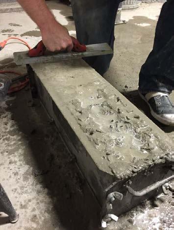
55 application of surface water (condition 4) Fig Finishing top surface of beam mold after second application of surface water (condition 4) Fig Rodding of beam surface after first surface finishing (condition 4) Fig Third and final application of surface water (condition 4) Fig Finishing beam surface (condition 4) 42

56 Fig Casting compression cylinders from same batch as beams (condition 4) Photos of the cast of the short beams, component

57 Fig Loading raw material for mixing Fig Air content measurement Fig Batch #1 mixture consistency Fig Slump test 44

58 Fig Beam mold preparation with standing water (condition 1) Fig Verifying standing water depth (condition 1) Fig Evenly placing concrete in beam mold with standing water (condition 1) Fig Top surface after concrete placement into beam mold with standing water (condition 1) 45

59 Fig Internal vibration of beam mold (condition 1) Fig Finishing surface of beam mold (condition 1) Fig Finished surface of beam mold (condition 1) Fig Concrete placement before top surface water application (condition 3) 46

60 Fig Surface water application (condition 3) Fig Top surface after first application of surface water (condition 3) Fig Internal vibration of beam mold (condition 3) Fig Striking off top surface (condition 3) 47

61 Fig Top surface before first rodding application (condition 3) Fig First rodding application (condition 3) Fig Top surface after rodding (condition 3) Fig Second application of surface water (condition 3) 48

62 Fig Finishing top surface after second application of surface water (condition 3) Fig Top surface after second application of rodding (condition 3) Fig Top surface after third and final application of surface water (condition 3) Fig Finished top surface (condition 3) 49

63 Fig Concrete placement into beam mold with standing water (condition 2) Fig Internal vibration of beam mold (condition 2) Fig Finished top surface (condition 2) Fig Concrete placement in beam mold before surface water application (condition 4) 50

64 Fig First application of surface water (condition 4) Fig Internal vibration of beam mold (condition 4) Fig Striking off top surface (condition 4) Fig First application of rodding (condition 4) 51

65 Fig Second application of surface water (condition 4) Fig Finishing top surface (condition 4) Fig Second and final application of rodding (condition 4) Fig Third and final application of surface water (condition 4) 52

66 Fig Finished top surface (condition 4) 53

67 CHAPTER 4: DESIGN AND ASSEMBLY OF THE NONDESTRUCTIVE EVALUATION METHODS In this section we describe the design and assembly of the hardware, software, numerical models, and tools we used to conduct the NDE experiments. Section 4.1 describes the two kinds of HNSW transducers assembled. Section 4.2 shows the setup of the ultrasonic pulse velocity (UPV) tests. Section 4.3 describes the results of the reliability test associated with one kind of transducers. Section 4.4 ends the chapter with some conclusions Highly Nonlinear Solitary Waves: Experimental Setup Two kinds of HNSW transducers were designed, assembled, and used. The first kind of transducers is schematized in Fig. 4.1a and it is indicated as the M-transducers. The other kind is illustrated in Fig. 4.1b, and it is indicated as the P-transducers. All transducers contained 16 stainless steel particles (AISI 302, McMaster-Carr). The second particle from the top was nonferromagnetic, whereas the other were ferromagnetic. The properties of the particles were: diameter 2a=19.05 mm, density ρ=7800 kg/m 3, mass m=27.8 g, modulus of elasticity E=193 GPa, and Poisson s ratio ν=0.25. Each chain was held by a Delrin tube (McMaster-Carr 8627K219) with outer diameter D 0 =22.30 mm and inner diameter slightly larger than the particles diameter in order to minimize the friction between the striker and the inner wall of the tube and to minimize acoustic leakage from the chain to the tube. The striker was driven by an electromagnet powered by a DC power supply. In the M-transducers a constant axial magnetic field was created along the chain and centered at the 9th particle using two identical permanent bridge magnets (McMaster-Carr 5841K55). A magnetic wire coil was wrapped around the tube and around the magnetic field in order to attain a magnetostrictive sensor (MsS) utilized to measure the propagation of the solitary waves traveling through the 9th particle. Finally, a mm thick aluminum sheet was glued to the tube s end to prevent the free fall of the particles. The falling height of the striker in M- transducers was 3.2 mm. As reported in (Ni, Cai and Rizzo 2013, Rizzo 2004, Rizzo and Lanza di Scalea 2007), magnetostriction can be used to excite and detect stress waves using the Faraday s law and the Villari s effect, respectively. In this study, we used the Villari s effect, which states that a pulse propagating through a ferromagnetic material modulates an existing magnetic field and generates voltage in the coils. In our experiments, the AISI 1020 was the magnetostrictive material subjected to the magnetic field induced by the magnets. One of the authors used MsS to excite and detected guided ultrasonic waves (Lanza di Scalea, Rizzo and Seible 2003, Rizzo and di Scalea 2006, Rizzo and Lanza di Scalea 2006). In the P-transducers, the sensing system consisted of a sensor-rod schematized in Fig. 4.1c and located in lieu of the 9 th particle of the chain. The sensor-rod consisted of a piezo ceramic disc of 19 mm diameter and 0.3 mm thickness. The disc (part number: SMD19T03112S), manufactured by Steiner & Martins Inc., was insulated with Kapton tape and embedded between two half rods. The rod was made from the same material as the beads, its mass m r = 27.8 g, height h r = 13.3 mm, and diameter D r = mm. These dimensions made the sensor-rod 54

68 approximately the same mass of each spherical particle. This was done to minimize any impurity in the chain that may have generated spurious HNSW. Finally, the falling height of the striker was 5 mm. (a) Electromagnet (b) Electromagnet Striker Striker Magnetostrictive Sensor Granular Chain PZT Sensor Granular Chain Positive (+) Window Aluminum Plate Delrin Acetal Resin Tube Aluminum Plate Negative (-) Delrin Acetal Resin Tube Specimen Specimen (c) Half Rod Isolation Tape PZT Isolation Tape Half Rod Fig. 4.1 (a) Schematic of the M-transducers, (b) schematic of the P-transducers, and (c) The schematic view of parts of the PZT sensor-rods. At the bottom of the six transducers an aluminum lamina was glued to the plastic tube in order to prevent the free fall of the particles. Several researches have been carried out to formulate the load-deflection behavior of the circular membranes (Timoshenko, Woinowsky- Krieger and Woinowsky-Krieger 1959, Eaton et al. 1999). In this study, we applied the 55

69 formulation of ref. (Eaton et al. 1999) to model the lamina in the transducers. Hereinafter, M1, M2, and M3 denote the M-transducers 1, 2, and 3, respectively while P1, P2, and P3 stand for P- transducers 1, 2, and 3, respectively. The transducers were controlled with a National Instrument-PXI (1042Q) unit running in LabVIEW and a DC power supply (BK PRECISION 1672). We used a Matrix Terminal Block (NI TB-2643) to branch the PXI output into four switch circuits. Figure 4.2(a) shows the diagram of the switch circuit. The symbols G, D and S represent the gate, drain, and source terminals of the MOSFET respectively. Although the MOSFET is a four-terminal device with source (S), gate (G), drain (D), and body (B) terminals, the body of the MOSFET is often connected to the source terminal. In the figure, EM1 through EM4 represent four electromagnets mounted above the chains. Switches 1 to 4 are digital switches, and if one of them is set as 1, the switch is on. Figure 4.2b shows the PXI, the power supply, and one of the switch circuits with a MOSFET and two terminal blocks. PXI (a) Gene rator NI TB 2643 Switch 1 Switch 2 Switch 3 Switch 4 G S D G D S G D S G S D EM1 EM2 EM3 EM4 DC Power (b) (c) (d) Fig. 4.2 The hardware: (a) the control circuit. EM1 to EM4 represents four electromagnets mounted on sensor 1 to sensor 4 respectively. Switches 1 to 4 are digital switches, and if one of them is set as 1, the switch will be turned on. (b) Left to right: photos of the PXI utilized in the experiments, the DC Power supply, used to provide electromagnet with direct voltage, and the switch circuit with a MOSFET and two terminal blocks Ultrasonic Pulse Velocity (UPV) Method: Experimental Setup For comparative purposes we applied the UPV. A function generator was used to excite a 5- cycle, 2 V peak-to-peak, 500 khz sine wave. Two Olympus V103-RM transducers were used to transmit and receive the waves, respectively. Two Olympus 5660C amplifiers were used to amplify the signals. It is known that in elastic homogeneous solid media, the longitudinal wave speed is given by: V UPV KE = d (4.1) ρ 56

70 where K=(1-ν)/((1+ν)(1-2ν)), and ρ is density of the medium. The static value of Poisson s ratio obtained from destructive test can be utilized in the absence of the dynamic Poisson s ratio (Malhotra and Carino 1991). To adhere to the results associated with the solitary wave testing, we considered ν=0.16. From Eq. (4.1): UPV d 2 = ρ / (4.2) E V K The ultrasonic wave velocity was calculated by considering the arrival time difference between the first peaks of the transmitted and the received signals Repeatability Tests Materials Testing To assess the repeatability of the solitary M-transducers, we tested them against the five different contact scenarios depicted in Fig The figure shows one of the four transducers suspended in air, above water, or in contact with soft polyurethane (SAWBONES, # ), hard polyurethane (SAWBONES, # ), and AISI 304 stainless steel. The nominal properties of the last three materials are listed in Table 4.1. One hundred measurements were taken for each medium for every transducer; hence, a total of 2,000 waveforms were analyzed. Figures 4.4(a) through 4.4(e) show the averaged time waveforms associated with the five different media. Three main wave packets are visible: the incident solitary wave (ISW), the primary reflected wave (PSW), and the secondary solitary wave (SSW). Fig. 4.3 Photo of the M-transducer in air, water, on soft polyurethane, hard polyurethane and stainless steel. 57

71 Table 4.1 Properties of the polyurethane and stainless steel. The values of polyurethane are from Biomechanical Test Material Sawbones. The parameters of stainless steel are from ASM material data sheet. Material Density (kg/m 3 ) Young s modulus (GPa) Soft polyurethane Hard polyurethane Stainless steel The time waveforms show both positive and negative voltage. When the solitary wave travels through the constant magnetic field induced by the permanent magnets, it increases the compression between two adjacent particles, and it creates a positive gradient of the magnetic flux, which in turn induces the positive voltage. When the pulse moves away, the dynamic compression disappears, a negative gradient of the magnetic flux is induced, and therefore, the output voltage has a negative gradient. The first pulse of the force profile represents the arrival of the ISW. The second, pulse is the PSW, i.e. the nonlinear solitary wave reflected from the interface with the tested media. Some results also show the presence of the SSW. The panel shows that the four sensors provide the same waveforms; therefore, the transducers are repeatable. Furthermore, there are some other characteristics associated with HNSWs in contact with various materials which are observable from these figures. These characteristics are: (1) the TOF PSW of HNSW decreases as the Young s modulus of interface material increases; Fig. 4.4 shows that the time distance between the incident pulse and the reflected pulse is smaller in the case of testing steel (Figs. 4.4(e) and (j)) compared to air, water, and the polyurethanes. (2) In the soft materials, due to larger deformations in the interface material compared to stiff materials, Secondary Solitary Waves (SSW) are generated and propagated in the chain of particles. SSW in the waveforms can be observed as the third pulse in the Force-time plot. According to Fig. 4.4, SSWs are not generated when the transducer is placed above steel. (3) The amplitude of SSW to Incident Solitary Wave (ISW) increases as the Young s modulus of interface decreases. This phenomenon is due to the large deformation of interface which causes a smaller amount of wave energy be reflected in the form of PSW, and consequently, a larger amount of wave energy be reflected in the form of secondary waves. This phenomenon is clearly observed in the integrated waveforms of Fig. 4.4 where in the case of air and water, the amplitude of SSW to ISW is even larger than amplitude of PSW to ISW, and this ratio vanishes to zero in the case of steel where no SSW forms in the chain. The integral of the voltage V(t), measured at the center of the 9 th particle, is proportional to the dynamic contact force F i.e. (Ni et al. 2013): F = K V () t dt (4.3) c where K c is a conversion factor expressed in N/V μs. 58

72 (a) Voltage (V) 0.6 V sensor1 sensor2 sensor3 sensor4 (f) Voltage Integral 10 V.Sec sensor1 sensor2 sensor3 sensor4 (b) (g) (c) (h) (d) (i) (e) (j) Time (ms) Time (ms) Fig. 4.4 Left column: averaged time waveforms when testing in air (a), water (b), soft polyurethane (c), hard polyurethane (d), and stainless steel (e). Right column: corresponding voltage integral. Each figure has four curves that are associated, from bottom to top, with the sensor 1 to 4, respectively. 59

73 Under the assumption that the numerical model presented later in Section mirrored the experimental setup, we calculated K c by computing the ratio of the numerical dynamic force to the experimental time integral both associated with the ISW, which is the only pulse not affected by the presence of any underlying material. For each transducer, the 500 experimental pulses were considered. The results are listed in Table 4.2, and they reveal that the values of K c are very similar. In fact, the difference between the smallest (6.42 N/V μs) and the largest (6.67 N/V μs) value is below 4% which proves the consistency of the assembled transducers. Moreover, within each transducer, the corresponding coefficients of variation, i.e. the ratio of the standard deviation σ to the mean value, are all below 5%, which is a good indicator of the repeatability of the incident pulse. Table 4.2 Calibration coefficient of the four magnetostrictive sensors. The coefficients are used to convert the voltage amplitude associated with the propagation of the solitary waves into Newton. Sensor Calibration Coefficient Standard Coefficient of Deviation Variation (%) The values of K c were then used in Eq. (4.3) to infer the dynamic force profile from the experimental time waveforms. Figures 4.4(f) to (j) represent the experimental force for each transducer in contact with the five different media. The ISW, PSW, and the SSW are visible. The latter is absent when steel was tested. The graphs confirm the repeatability of the transducers. The TOF PSW consists of three parts, one part is the travel time (T i ) from the 9 th to the last particle of the chain; the second part is the contact time (T c ) of the last particle with the tested specimen (wall); and the third part is the travel time (T p ) from the last particle to the 9 th particle. So the TOF PSW can be explained as the following: TOFPSW = Ti + Tc + Tp (4.4) When interacting with soft interface, SSW will be generated. TOF PSW consists of two parts, the first part is TOF PSW and the second part is the contact time between the end particle and tested media, so the TOF SSW can be presented as following: TOF = T + T ' (4.5) SSW PSW c Same as the T c, T c is also related to the tested material. If the specimens become stiffer, the values for Young s modulus increase, consequently the contact time T c and T c decrease. 60

74 (a) (b) Fig. 4.5 Time of flight associated with the (a) primary reflected wave (TOF PSW ) and (b) the secondary reflected solitary wave (TOF SSW ) as a function of the five different media in contact with the solitary wave transducers. Figure 4.5 shows that the TOF PSW and TOF SSW decrease as the values for Young s modulus of the specimen increase. Not shown here, we also found that with the increase of the specimen stiffness, the amplitude of the PSWs increases and the amplitude of the SSWs decreases until it disappears as in the case of the steel specimen. Particularly, in the case of soft polyurethane the SSW is evident. The data relative to the four sensors and the 5 different media are summarized in Table 4.3. From Fig. 4.5 and Table 4.3, it is observed that the values of the TOF PSW s and TOF SSW s are decreasing as the tested media becomes stiffer. The four transducers provide almost identical results. The biggest difference among the four sensors is 6.0% when testing steel, whereas the smallest difference is 0.08% when there was no material in contact with the transducer. Moreover, both features are repeatable because of the corresponding coefficients of variation are quite small. For the TOF SSW, the coefficients of variation are all below 0.4%, and for the TOF SSW, they are not more than 5% 61

75 Table Average TOF PSW and TOF SSW and corresponding standard deviations measured when testing the five different media. TOF PSW (ms) TOF SSW (ms) Medium Sensor Coefficient of Coefficient of Mean Std Mean Std Variation (%) Variation (%) Air Water Soft Polyurethane Hard Polyurethane Stainless Steel N/A N/A N/A N/A N/A N/A N/A N/A N/A N/A N/A N/A Numerical Model In order to interpret and predict the experimental results, a numerical model was implemented. The partial differential equation of the motion of 1D HNSW in the numerical method can be determined by using Lagrangian description of particle dynamics: [ ] [ ] 2 3/2 3/2 tt n n 1 n + n n+ 1 + m u = Au u Au u (4.6) where u i is the i th particle displacement, [x] + denotes max(x,0), and A is a stiffness constant that depends on the properties of the spheres or the property of the material in contact with the chain. By solving Eq. (4.4), the time history of the n th particle s oscillation is obtained based on which HNSW can be characterized. It should be noted that in this Equation, it is assumed that the displacement of wall is zero. Figure 4.6 shows the force profiles predicted by the numerical model when the five different interfaces were considered. Figure 4.6 demonstrates that the waveform is highly sensitive to material type i.e. material with higher Young s moduli have smaller TOF PSW, and larger PSW/ISW ratios in both numerical and experimental results. It is also observed that the magnitude of secondary waves to incident waves increases as the Young s modulus of the material decreases. Secondary wave amplitude is zero for steel and its maximum value is reached when testing in air. When the HNSW reaches to the top bead, due to small gravity precompression, the first and the second bead are separated, and they again collide; hence, a small bump propagates in the chain of beads. These bumps are observable in both experimental results (Fig. 4.4) and numerical simulation (Fig. 4.6). From Fig. 4.6, it is also observed that PSW 62

76 and SSW, in case of air and water, have two peaks. This phenomenon happens when the wall is very soft, and the separation of the last bead cause its adjacent beads to collide at different times. Fig. 4.6 Numerical results. Force profile of the HNSWs propagating through the 9 th particle of a chain of steel spheres in contact with the five different media considered in the experiments. Figure 4.7 shows the variation of TOF PSW as a function of the Young s modulus and the Poisson s ratio of the contact material. In this figure, it is observed that Poisson s ratio has a negligible effect on the variation of the TOF PSW ; on the contrary, the Young s modulus has a significant impact on time of flight when E<100 GPa. It is also observed that the Poisson s ratio does not affect significantly the PSW/ISW ratio. Fig. 4.7 Numerical results. TOF PSW as a function of the Young's modulus and Poisson's ratio of the material in contact with the chain of particles. 63

77 Fig. 4.8 Numerical results. Ratio PSW/ISW as a function of the Young's modulus and Poisson's ratio of the material in contact with the chain of particles. The magnitude of the PSW to the ISW ratio is shown in Fig. 4.8 for various Young s modulus and Poisson s ratio. From this figure, it is observed that the ratio of the PSW to the ISW increases as Young s modulus increases until it reaches a threshold value. From this figure, it is also observed that the Poisson s ratio does not affect the PSW/ISW ratio. Similarly, Fig. 4.9 shows the magnitude of the SSW to the ISW ratio. The figure shows the amplitude of SSW has a descending trend, and the SSW is not generated when E>50 GPa, and similar to Fig. 4.8, the effect of the Poisson s ratio is far less than the Young s modulus. Fig. 4.9 Numerical results. Ratio SSW/ISW as a function of the Young's modulus and Poisson's ratio of the material in contact with the chain of particles. 64

78 Table 4.4 presents the TOF PSW s of both experimental and numerical, and the difference represents the difference between numerical results and experimental results. For air and water, their stiffness are related to the aluminum plate at the bottom of the chain, and they are not elastic media so the results are quite different from what we get from the experiments. The experiments completed in air and water are just used to certify the repeatability and stability of the four sensors. For the other three media, the differences between numeric and experiments are much smaller. Table 4.4 Experimental and numerical TOF PSW and their difference. Medium Numerical TOF PSW (ms) Experiment al TOF PSW (ms) Coefficient of variation (%) Air Water Soft polyurethane Hard Polyurethane Steel Concrete Testing: Setup The concrete samples tested during this phase of the project were cast by another research group in August 2014, i.e. prior to the beginning of this project. Table 4.5 Parameters obtained from ASTM C469 and ASTM C39 Samples Compressive Young s Modulus Poisson s Strength (psi) (GPa) Ratio C C C Table 4.6 Size and weight of tested concrete slab samples Dimension Mass Slab (kg) length (cm) width (cm) height (cm)

79 Based on data provided to us and based on unconfined compression tests (ASTM C469), split cylinder tests (ASTM C469), and compressive strength tests (ASTM C39), the properties of the concrete batch are listed in Table 4.5, whereas the dimension and weight are listed in Table 4.6. We placed the four identical transducers on the specimens to be tested as shown in Fig Fig Experimental setup The photos of the setup associated with the UPV test are instead presented in Fig Figure 4.11(a) and (b) are the transmitter and the receiver, respectively, of which both are longitudinal ultrasonic transducers (Olympus V103-RM). Due to the heterogeneous property of concrete, we tested five different points 10 times as shown in Fig. 4.11(c), and calculate the average value of all the measurements. (a) (b) (c) Fig The experimental setup and schematic of the UPV test. Figure 4.12 shows the transmitted ultrasonic pulse and the received pulse waveforms. For regular concrete, the pulse velocity is typically 3700 to 4200 m/s, and the velocity of the ultrasonic pulse depends on the elasticity properties and density of the specimen. 66

80 Amplitude (V) Transmitted wave Time (us) Received wave Transmitted Received Fig Example of transmitted (blue solid line) and received (dashed red line) signals in the UPV testing of the concrete slabs. The time interval between the first peak of both lines was considered. From the ASTM C39 and C469 tests on the samples, C-28-1, C-28-2 and C-28-3, we assumed the Poisson s ratio, µ=0.16, combined with the measured density ρ, we can calculate the dynamic modulus of elasticity by using Eq. (4.2). ACI section correlates the dynamic modulus of elasticity and the compressive strength of concrete. Since we got the compressive strength of the concrete in the lab by ASTM C39, the dynamic modulus of elasticity can be predicted by the following: E C = 33( ω ) f 1.5 ' c where is the unit weight of concrete in lb/ft 3 (90~155 lb/ft 3 ), and f c is the compressive strength in psi. The density matrix D is calculated, and the designed compressive strength f c was obtained by ASTM C Concrete Testing: Results Figure 4.13 shows the waveform obtained by averaging the 100 measurements on sample 4. This figure shows that despite of inhomogeneous nature of concrete and the use of different transducers at different slab locations, the waveforms are almost identical. (4.7) 67

81 Voltage integral 10 V.Sec sensor1 sensor2 sensor3 sensor Time (ms) Fig The output voltage integral waveforms of the four sensors, of which the top curve is the signal obtained by sensor 4 and the bottom curve is obtained by sensor 1. TOF (ms) TOF (ms) (a) Slabs Number (b) sensor1 sensor2 sensor3 sensor4 sensor1 sensor2 sensor3 sensor Slabs Number Fig Averaged value of the 100 measurements taken by the four transducers at four different surface location of the eight slabs. (a) Feature of the TOF PSW ; (b) feature of the TOF SSW. The small vertical bars represent the standard deviation of the experimental data. 68

82 Table 4.7 Eastimating Young's Modulus of Concrete slab samples using HNSW-based sensors, Ultrasonic Testing, and Destructive testing Slab Sensor TOF PSW E d (HNSW) Averaged E d (HNSW) E d (Ultrasonic) E (ACI Section 8.5.1) ms GPa GPa GPa GPa Average * * Outliers including the values of slab 1 and 3 are not used in the average value. Figure 4.14 shows instead the average time of flight between PSW and SSW, and the standard deviation. The scatter of the features values is below 5%, and it is likely due to the intrinsic slight differences among the transducers and the heterogeneity of the samples surface. Other 69

83 factors include the intrinsic differences among the transducers as discussed previously and the intrinsic heterogeneity of concrete. In fact, the presence of coarse aggregates, voids, blisters, and the rough surface may have some impacts on the solitary wave features. Typically, the aggregates have larger Young s modulus than the cement paste; consequently, the TOF PSW and TOF SSW will be smaller than the values of the concrete. On the contrary, if many voids are located close to the chain/concrete interface, the values of the TOF PSW and TOF SSW will be larger than the values of the concrete with no voids. The TOF PSW was used to estimate the Young s modulus of the concrete samples. Using the experimental values of the solitary wave features into the numerical model, the experimental moduli are presented in Table 4.7 after assuming the Poisson s ratio equal to The HNSWs-based predictions of the Young s modulus range from 16.3 GPa to 38.4 GPa, and the average value is 27.3 GPa. The value for modulus from UPV test range from 24 GPa to 29.1 GPa, and the modulus calculated from the empirical equation range from GPa to GPa. The moduli we retrieved from HNSW-based sensors, UPV test and the empirical equation from ACI Section are all dynamic Young s modulus E d. The static Young s modulus of the concrete, E s, is tested by ASTM C469, and E s =25 GPa. Several attempts have been made to correlate static (E s ) and dynamic (E d ) moduli for concrete and the simplest of these empirical relations is proposed by Lydon and Balendran (Lydon and Balendran 1986b, Popovics, Zemajtis and Shkolnik 2008a): E s = 0.83E (4.8) d In our experiments with the solitary wave transducers, we regarded the modulus of the slab 1 and 3 as outliers, and then the average dynamic Young s modulus will be 30.8 GPa. The average young s modulus predicted by the empirical equation, with the 28-day compressive strength f c got from ASTM C39, is 29.98, which is very close to the result of HNSW experiment. Table 4.7 reports the E d HNSW computed from all four transducers for all 8 samples. By looking at the eight readings from the same transducer, it is evident that the scatter of the data is much higher than the variability of the individual transducer. This suggests that the heterogeneous surface of the samples might have scattered the data. To support this hypothesis, Fig displays a close-up view of the surface of slab 1, slab 3, and slab 4. Many voids are visible on slabs 1 and 3. These voids (bugholes) typically result from the migration of entrapped air and to a less extent water, to the fresh concrete interfaces. These voids and the roughness of the surfaces may weaken the local stiffness of the concrete or may influence the dynamic interaction at the material/transducer interface. 70

84 (a) (b) (c) Fig The surface of slab (a) 1, (b) 3 and (c) 4. There are many voids on the surface of slab 1and 3, on the contrary, slab 4 has a much smoother surface with fewer voids. The ultrasonic wave velocity was calculated by considering the arrival time difference between the first peaks of the transmitted and the received signals. The pulse velocity, the dynamic modulus of elasticity computed from Eq. (4.1), and the static modulus derived from Eq. (4.8) are listed in Table 4.8. Each value is the average of the five measurements taken from each slab. The results show that the variation among the moduli is very small, and the slabs 1 and 3 are not outliers. The reason is that the UPV test measures the pulse velocity of the waves traveling through the specimen, and therefore, it is less susceptible to surface conditions. Table 4.8 UPV test. Velocity of the longitudinal bulk wave and predicted dynamic and static modulus of elasticity. Slab Number Average Bulk E UPV d (GPa) E UPV s (GPa) Wave Velocity (m/s) Average Summary The moduli obtained from the different testing methods are presented in Table 4.9 and displayed in Fig The HNSWs-based prediction ranges from 13.5 GPa to 31.9 GPa, the value for modulus from the UPV test range from 19.9 GPa to 24.2 GPa, and the modulus calculated from the empirical equation range from 32.8 GPa to 33.7 GPa. In the figure, the average values and the corresponding standard deviations are presented. There are small differences in the modulus of elasticity of the slabs measured by the UPV test. The differences among the eight slabs are mainly caused by the following three reasons: first, the rough surface of the specimen changes the thicknesses or the path lengths in different testing areas, and this problem results in inaccurate path length L when calculated the pulse velocity; second, the 71

85 aggregates are important factor for the pulse velocity. Their sizes, types, and content can affect the test results; third, the rough surface results in insufficient contact with the commercial transducers, and a weaker pulse velocity will be received by the transducer; consequently, the onset of received signals may be difficult to be figured out. Based on the UPV measurements, the average dynamic modulus of elasticity of the 8 concrete slabs is 26.3 GPa, and its corresponding static modulus is equal to 21.8 GPa. Table 4.9 Concrete tests. Estimated static modulus of elasticity of the test samples using two destructive and two nondestructive methods. Nondestructive methods Slab Number HNSW E s (GPa) UPV E s (GPa) Destructive methods * 20.7 ASTM C469 ACI E Sample s E s (GPa) (GPa) * Average Average * The results of slabs 1 and 3 were not used in the average. Fig The average estimated static modulus of elasticity and the corresponding standard deviations of the four different methods. The results relative to the ASTM C469 conducted after 28 days from casting, the modulus of elasticity of the batch ranges from 25.5 to 28.9 GPa. Figure 4.17 shows that the standard deviation of the ACI equation is the smallest among the four methods. Furthermore, the modulus of elasticity estimated via the UPV is smaller than the other methods, while HNSW-based transducers provide the static modulus of elasticity very close to the ASTM C469. The difference between HNSW-based method and the ASTM is about 5%, while the difference between ASTM and the UPV method and the empirical equation of the ACI 318 are 20% and 23%, respectively. 72

86 Based on the findings presented in this chapter and some of the preliminary determinations not presented in the report, the following conclusions can be drawn: The variation among the four M-transducers is ±3% from the mean value; this means that the design of the transducers is repeatable. The standard deviation of the measurements associated with the same M-transdcuer at a given contact condition between the chain and the material is in the order of 0.4% from the mean value; this implies that the methodology is highly repeatable. The parameter of the time of flight can neatly discriminate the five contact conditions investigated in this chapter. The numerical model portrays/predicts the experimental results within a margin that is inversely proportional to the Young s modulus, i.e. the softer is the material in contact with the wall, the larger is the discrepancy between the numerical and the experimental results. To reduce the mismatch between the numerical and the experimental data, the numerical model should include attanutation and dissipation and it should also account for viscoelastic phenomena that may occur. The time of flight is the most reliable HNSW feature to be used to assess the Young s modulus. The Poisson s ratio does not influence the results significantly; this means that a typical Poisson s ratio can be assumed for concrete, let say in the range [ ], without compromising the accuracy of the estimation of the concrete modulus. When testing concrete, the TOF of the SSW is less reliable than the TOF of the PSW. The presence of voids and bugholes on the surface of concrete may affect the solitary waves readings; however, more studies are necessary to generalize and to verify this conclusion. Not shown in the report, the features associated with the amplitude of the solitary waves are not as reliable as the features associated with the time of flight. The dynamic modulus of elasticity predicted with the solitary waves is closer than that obtained by the UPV. The main advantages of operating HNSW-based test is that its implementation is fast and easy; hence, it is possible to carry out a large number of tests and take the average of the value of modulus of elasticity estimated from each observation. Another advantage of the HNSW-based method for evaluating the modulus of elasticity of the specimens is that the value obtained by this method is less susceptible to any damage and/or the presence of reinforcing steels existing inside the element. For example, cracks and dense reinforcing steel may cause refraction and dispersion of the ultrasonic waves while this problem does not affect the results of the HNSWbased transducers. 73

87 CHAPTER 5: NONDESTRUCTIVE AND ASTM TESTING (28 DAYS TESTS) In this section we present the results of the nondestructive and destructive testing conducted on the concrete samples fabricated in this project. Section 5.1 briefly describes again the concrete cylinders and the test protocols; Section 5.2 illustrates the results with the M-transducers; Section 5.3 illustrates the results with the P-transducers; Section 5.4 describes the destructive tests conducted using ASTM procedures; Section 5.5 summarizes the findings of the UPV method; Section 5.6 describes the computation of the concrete modulus with all the four methods. A brief summary of the short beam samples and the corresponding experimental protocol is given in Section 5.7, whereas the experimental results relative to the solitary wave based transducers are presented in Section 5.8. Section 5.9 presents the results of the UPV applied to the short concrete beams. Finally, Section 5.10 summarizes the main findings and the main outcomes of this part of the project 5.1. Concrete Cylinders and Test Protocol As said in Chapter 3, nine concrete cylinders were molded and tested using the NDE methods of the solitary waves and of the UPV. The cylinders were 6-in. diameter by 12-in. Three w/c, namely 0.42, 0.45, 0.50, were considered. The information about the concrete specimens ratios is summarized in Table 5.1. To ease the identification of each sample, we labeled them with 4 digits. The first digit is the letter C which indicates the cylindrical shape of the specimens; the next two digits represent the w/c ratio; finally, the fourth digit is a letter A, B, or C that indicates the individual specimen. Table 5.1 The detailed information of the concrete cylinders Number of Batch w/c ratio Cast date Samples label cylinders C42A, C42B, C42C 06/09/ C45A, C45B, C45C Tuesday C50A, C50B, C50C NDE Test date 07/07/2015 Tuesday Three M-transducers and three P-transducers were used to assess the cylindrical specimens. Each transducer was used to test all nine specimens, i.e. the experiments were conducted in a round-robin fashion, in order to prevent any bias in the results that may have stemmed from the transducers. For each test, 50 measurements were taken. Hereinafter, M1, M2, and M3 denotes the M-transducers 1, 2, and 3, respectively while P1, P2, and P3 stand for P-transducers 1, 2, and 3, respectively. The cylinders were tested using the HNSWs immediately after curing the samples at 95% relative humidity for 28 days. Figure 5.1 shows the setup when the M-transducers were placed above the specimens. Posts and clamps were used to hold the transducers. Similarly, Fig. 5.1b shows a P-transducer. 74

88 (a) (b) Fig. 5.1 Typical (a) M-transducers set-up, (b) P-transducers set-up The UPV test was performed by measuring the velocity of the wave propagating along and perpendicular to the longitudinal axis of the cylinders as shown in Fig The average of 300 time waveforms was recorded for each cylinder in each direction to increase the signal-to-noise ratio (SNR). We tested the cylinders along two directions to avoid any issue associated with wave attenuation due to the aggregates and to avoid any issue related to the curved shape of the surface. Prior to using the UPV, the cylinders were cured at room temperature under typical room humidity for 1 day. After the experiments the cylinders stayed at the same temperature and humidity conditions. Fig. 5.2 UPV testing: (Left) along and (Right) perpendicular the axis of the cylinders 5.2. Results of the M-Transducers Figures 5.3a and 5.3b show the voltage waveforms and the corresponding integrated values, respectively, associated with one of the 50 measurements taken with the M1 placed above specimens C42A, C45A, and C50A. Figures 5.3a and 5.3b are magnified in Figs. 5.3c and 5.3d, respectively to show the changes in the TOF of the first reflected pulse, due to changes in the w/c of the concrete. The first pulse is the ISW whereas the second pulse is the PSW reflected from the chain-concrete interface. The figures suggest that the TOF of the PSW increases with the increase in w/c. In the previous chapter, it was said that the numerical model predicts that longer 75

89 TOFs are generated when testing the samples with smaller modulus of elasticity. The experimental data visible in Fig. 5.3 confirm the numerical prediction. (a) W/C=42% W/C=45% W/C=50% (b) W/C=42% W/C=45% W/C=50% Voltage (V) 0.8 V Integrated Voltage (V.ms) Time (ms) Time (ms) (c) W/C=50% W/C=45% W/C=42% (d) W/C=50% W/C=45% W/C=42% Vlotage (V) 0.8 V TOF TOF Integrated Voltage (V.ms) TOF TOF TOF TOF Time (ms) Time (ms) Fig. 5.3 (a) Voltage waveform of M1 for the cylinders with different w/c; (b) Integrated voltage waveform of M1 for the cylinders with different w/c; (c) A close-up view of the voltage waveform of M1 for each batch; (d) A close-up view of the integrated voltage waveform of M1 for each batch. w/c Table 5.2 The TOF and standard deviation values of the M-transducers Cylinder M1 M2 M3 TOF (ms) STD (ms) TOF (ms) STD (ms) TOF (ms) STD (ms) C42A C42B C42C C45A C45B C45C C50A C50B C50C Table 5.2 summarizes the results of the M-transducers. It lists the TOFs of the PSW. Each value is the average of the fifty measurements. The corresponding standard deviations are also listed. The data confirm that the TOF increases with the increase of the w/c ratio, and the 76

90 variations relative to the cylinders with the same ratio vary much less than the values across the different ratios. The standard deviation of all TOFs is below ms, which results in the coefficient of variation, also known as relative standard deviation, below 0.3%. This demonstrates that the measurement setup is very repeatable. The data listed in Table 5.2 are displayed in Fig The values of 2σ are represented in the vertical error bars, and demonstrate that the standard deviations are smaller than the changes in the TOFs due to the w/c ratio; furthermore, the TOF increases slightly as the w/c increases. Fig. 5.4 TOFs and associated standard deviations obtained from the three different batches Results of the P-Transducers Figure 5.5a shows one of the fifty waveforms recorded with P1 above C42A, C45A, and C50A. Fig. 5.5b is a close-up view of Fig. 5.5a, in order to emphasize any variation in the TOFs. Similar to Fig. 5.3, a change in the TOFs of the primary reflected wave is observed, and its value increases with an increase in w/c ratio. The overall results relative to the TOF are summarized in Table 5.3. A comparison of the results presented in this table with those of Table 5.2 reveals that the values of TOF in both transducers are pretty close. The coefficient of variations ranges from 0.2% to 0.9%, which proves the high repeatability of the P-transducers as well. (a) W/C=42% W/C=45% W/C=50% (b) Voltage (V) 5 V Time (ms) Fig. 5.5 (a) Time waveform recorded by P1 for the cylinders with different w/c; (b) A close-up view of the time waveform and the TOF of each w/c ratio. 77

91 Table 5.3 The TOF and standard deviation values measured by P-transducers for different batches P1 P2 P3 w/c Cylinder TOF (ms) STD (ms) TOF (ms) STD (ms) TOF (ms) STD (ms) C42A C42B C42C C45A C45B C45C C50A C50B C50C Figure 5.6 shows the TOFs of different batches and different cylinders. To ease the comparison between the readings of the M-transducers with the readings of the P-transducers, we kept the same vertical axis scale. Here, the ascending trend is more obvious than that in Fig. 5.4 although the error bars are larger. Therefore, the P-transducers are more sensitive to the stiffness change of the concrete surface; however, they show a larger standard deviation. We believe that the effectiveness of the P-transducers with respect to the M-transducers is due to the following factors: 1) the small horizontal oscillations of the 9 th bead may affect the voltage output of the MsS; the sensor-rod in the P-transducers is less prone to this horizontal oscillation because of the geometry of the rod. 2) The MsS averages the dynamic force associated with the solitary wave across the permanent magnetic field induced by the permanent magnets. The sensor rod instead senses the dynamic field at the location of the PZT. 3) The aluminum lamina under the P-transducers contained a through-thickness hole that put the last particle of the chain in contact with the concrete. Fig. 5.6 TOF and associated standard deviation values measured vs w/c ratio Young s Modulus Computation Destructive Testing Using ASTM C39 and C469 78

92 Three specimens from each batch were tested according to ASTM C39 and C469 for the destructive testing of the concrete samples. The samples were tested after curing for 28 days at 70 F and a relative humidity of 95%. These tests are conventionally used to estimate modulus of elasticity, Poisson s ratio, and ultimate strength of the cylinders. The results of these tests are presented in Table 5.4 and displayed in Fig The average modulus of elasticity was 38.6 GPa, 35.7 GPa, and 32.4 GPa for w/c ratio of 0.42, 0.45, and 0.50, respectively. The testing of the cylinders was performed when the specimens were saturated in accordance with ASTM specifications. The NDT testing was performed on dry specimens. W/C Table 5.4 Concrete parameters obtained through ASTM C39 and ASTM C469 Sample Average Relative Relative Elastic Compressive compressive standard Average standard Modulus Strength (MPa) Strength deviation (GPa) deviation (GPa) (MPa) (%) (%) C42A C42B C42C C45A C45B C45C C50A C50B C50C As expected, the ultimate compressive strength and the modulus of elasticity decrease with an increase in the w/c ratio. If the values associated with w/c=0.42 are taken as the reference, the elastic modulus decreased by 7.5% and 9.2% for w/c ratios of 0.45 and 0.50, respectively. Similarly, the compressive strength decreased by 2.8% and 12.6% for w/c=0.45 and w/c=0.50, respectively. Fig. 5.7 The modulus of elasticity and associated standard deviations measured in accordance with the ASTM C UPV Testing UPV testing was performed after curing the samples for 28 days and keeping them for 1 day in a laboratory at room temperature. Figure 5.8 shows one of the waveforms recorded. The 79

93 transmitted and the received pulses are clearly visible. The travel time was determined by mesuring the onset of the two pulses. Fig. 5.8 A typical waveform recorded from UPV test Using Eqs. (4.1) and (4.2), the modulus of elasticity of the cylinders was estimated. For the Poisson s ratio, we adopted the typical value of 0.2. The results are presented in Table 5.5. This table shows that an increase in w/c ratio results in a smaller wave velocity and modulus of elasticity. Moreover, the variation within the same batch is very small and below 1.9%. Figure 5.9a shows the computed wave velocity for the cylinders with different w/c ratios, whereas Fig. 5.9b presents the computed modulus of elasticity of the samples. Overall, there is not a significant difference between the longitudinal and the transverse measurements, which suggests that our setup was reliable. When compared to the data presented in Table 5.5, the data presented in Table 5.5 and Fig. 5.9b reveal that the UPV underestimates the Young s modulus. It would be anticipated that this modulus would be higher than the static modulus measured in accordance with ASTM C469. One contribution factor could be that the specimens were dry when tested nondestructively, and the specimens were saturated when tested in accordance with ASTM C469. w/c Cylinder Table 5.5. The modulus of elasticity of each cylinder obtained by the UPV test Average modulus of Pulse Velocity (m/s) Modulus of elasticity (GPa) elasticity (GPa) Longitudinal Transverse Longitudinal Transverse Longitudinal Transverse C42A C42B C42C C45A C45B C45C C50A C50B C50C

94 Fig. 5.9 (a) The measured UPV wave velocities of the cylinders. (b) The estimated modulus of elasticity of cylinders with different w/c from UPV test HNSW-based Transducers The numerical model described in Section was used to predict the TOF of the HNSWbased transducers as a function of the dynamic modulus of elasticity and the Poisson s ratio of the material in contact with the chain. The results are presented in Fig. 5.10: a plot of the TOF as a function of the modulus of elasticity at ν=0.20 is shown in Fig. 5.10b. According to Fig. 10a, the variation of the TOF due to the Poisson s ratio is far less than the effect of the modulus of elasticity. For example, if TOF= ms, the modulus of elasticity corresponding to ν=0.15 and ν=0.35 are 52.6 GPa and 47.2 GPa, respectively, which shows only 10% changes. In field applications, the value of the Poisson s ratio of the material is unknown. If concrete is the material to be tested, a value between 0.15 and 0.20 is reasonable to estimate accurately the modulus of elasticity. In this study, the value of ν=0.20 was adopted. (a) (b) = TOF (ms) E (GPa) Fig Numerical model. (a) TOF as a function of the dynamic modulus of elasticity and the Poisson s ratio; (b) TOF as a function of the modulus of elasticity when ν=

95 In the NDE method investigated in this project, we estimated the modulus of the samples by intersecting the value of the TOF measured with the HNSW-based transducers to the curve of Fig. 5.10b. For illustrative purposes, this figure shows the modulus corresponding to two experimental TOF. The graph demonstrates that when the modulus of elasticity of the probed specimen is higher than 25 GPa, small differences in the measurement of the TOF (in this example 3.2%) yields a large change in the estimated modulus (in this example 60%). This implies that high accuracy is required in the measurement of the solitary wave parameter. The dynamic modulus of elasticity E d was then converted into the static modulus of elasticity E s using the empirical formula (4.8) proposed by Lydon and Balendran (Lydon and Balendran 1986a, Popovics, Zemajtis and Shkolnik 2008b). The static moduli estimated by using the M-transducers are presented in Table 5.6. They are based on the values of the TOFs presented in Table 5.2. The values were then averaged and reported on the rightmost column of the table. The column shows that an increase in the w/c ratio decreases the static modulus. Similar to Table 5.6, Table 5.7 presents the modulus estimated using the measurements of the P-transducers. Overall the findings from the two kinds of the transducers are similar. Table 5.6 The estimated modulus of elasticity of each cylinder obtained by the M-transducers E (GPa) based on TOF of Primary Waves w/c ratio Cylinder Average M1 M2 M3 M-transducers Samples average 42A B C A B C A B C Table 5.7 The predicted modulus of elasticity of each cylinder through P-transducers E (GPa) based on TOF of Primary Waves w/c ratio Cylinder Average P1 P2 P3 P-transducers Samples average 42A B C A B C A B C Few reasons explains the differences in the experiments: the inhomogeneous properties of concrete, the voids on the surface of the cylinders; the location of the transducers above the sample. Because the aggregate used in the batches was limestone (E s ~50 GPa), which has a 82

96 bigger modulus of elasticity than the cement paste, if the transducer is placed at the top of an aggregate, the estimated modulus of elasticity will be larger than the case of being placed on the cement paste Comparison from All Methods Table 5.8 and Fig summarize the estimated modulus of elasticity using the different testing methods adopted in this study. The results from the HNSW transducers are the average of the three M- and the three P-transducers, and for each transducer, we used the average value of fifty measurements. The results of the UPV test are the mean of the axial and transverse measurements. If we consider ASTM C469 as the reference method, the deviations of the M- transducers from the reference are 0.8%, 3.1%, and 4.9% for w/c ratio equal to 0.42, 0.45, and 0.50, respectively; the deviations of the P-transducers from the reference are 6.5%, 5.0%, and 1.9% for w/c ratio equal to 0.42, 0.45, and 0.50, respectively while these values for the UPV method are 10.0%, 14.1%, and 12.9%, respectively. Table 5.8 The modulus of elasticity estimated via various methods w/c ratio Modulus of elasticity (GPa) ASTM C469 M-Transducers P-transducers UPV test Fig shows the static modulus as a function of w/c ratio for each method. It is clearly visible that all the methods detect the degradation of the concrete properties due to the increase of the amount of water. It is evident that the moduli estimated by the HNSW-based method are the closest to the data provided by the ASTM C469. Fig The Average modulus of elasticity of various studied methods. 83

97 5.5. Short Beams with Standing Water During Concreting As detailed in Section 3.2, we cast short concrete beams under the following four different conditions: Condition 1: 0.5 in. of standing water at the bottom of the form. Condition 2: 0.25 in. of standing water at the bottom of the form. Condition 3: finish and equivalence of 0.1 in. of rainfall into the surface Condition 4: finish and equivalence of 0.15 in. of rainfall into the surface In all beams the w/c ratio before introducing each field condition above was equal to The four conditions were reproduced onto four different specimens, resulting in a total of 16 test samples. Two specimens of each condition were cast on 23 June, and two more specimens of each condition were cast on 24 June. For convenience the scheme of the samples (Fig. 5.12) and the detailed information (Table 5.9) are given here again. Table 5.9 shows the characteristics and notation of the beams with different conditions. Two batches having the same concrete mixture design were prepared each day and are indicated as batch #1 and batch #2. From the first batch, the samples with condition 1 and condition 3 were prepared. From the second batch the samples with condition 2 and condition 4 were prepared. The beams were cured for 28 days at 70 F and at relative humidity of 95%. They were then immediately tested with the HNSWs transducers at room conditions and were tested with the UPV the day after. They were then stored at room temperature indefinitely. (a) (b) (c) Fig (a) condition 1: 0.5 in excessive water at the bottom of the beam, (b) condition 2: 0.25 in excessive water at the bottom of the beam, (c) condition 3: 0.10 in excessive water at the top of the beam, (d) condition 4: 0.15 in excessive water at the top of the beam. (d) 84

98 Table 5.9 Labels of the short beams. Cast Date Beam Label Batch Condition 6/23/2015 B1-A 1 B1-B 1 B3-A 3 B3-B B2-A 2 B2-B 2 B4-A 4 B4-B 6/24/2015 B1-C 1 B1-D 1 B3-C 3 B3-D B2-C 2 B2-D 2 B4-C 4 B4-D HNSW Results Both top and bottom surfaces of the beams were tested using the M- and the P-transducers. Each kind of transducers was placed on the surface simultaneously, and fifty measurements were recorded by each transducer and used in the signal processing. Fig shows the setups relative to the solitary wave measurements. It can be seen that each sample was tested simultaneously with three transducers and at three different locations. This translates in time and cost-savings. Fig (a) Placing M-transducers on the beams; (b) placing P-transducers on the beams 85

99 The results associated with the time of flight of the primary solitary wave is listed in Table 5.10 for both kinds of transducers along with the corresponding modulus computed using the approach described previously. The mean values are presented in the row highlighted in green. We observe that the readings from the P- and the M- transducers are very close to each other. Moreover, we notice that the modulus estimated on the top of the surface was higher than the corresponding value at the bottom where the standing water was located before pouring the concrete. We believe that the explanation is on the fact that: 1) the concrete was vibrated after pouring it in the formworks; 2) the weight of the concrete displaced the standing water from the bottom to the top as it is clearly visible in Fig The four bottom rows of Table 5.10 compare the estimates of the solitary wave transducers in the short beam with the corresponding values obtained in the cylinders with the three w/c, summarized in Table 5.8, and discussed in Section 5.4. The comparison of the data reveals that the beams Young modulus was comparable to the modulus of the cylinders with high w/c. The data suggests that the Young s modulus estimated in the top surface of the short beam contained an amount of water superior to the w/c=0.5, whereas the bottom surface of the short beam contained an amount of water equivalent to w/c= So, the HNSW transducers were able to capture the circumstance that the short beams were corrupted by water in excess. DATE Batch 06/23/2015 Batch #1 06/24/2015 Batch #1 Table 5.10 The TOF and modulus of elasticity of the beams in which condition 1 was imposed TOP SURFACE BOTTOM SURFACE M-trans. M- M-trans. M- P-trans. Sample P-trans. P-trans. TOF trans. TOF trans. TOF TOF (ms) E (GPa) (ms) E (GPa) (ms) E (GPa) (ms) B1-A B1-B B1-C B1-D Average (GPa) Short beam w/c=0.42 Condition 1 P-trans. E (GPa) Average w/c=0.42 short beam cond. 1 Average w/c=0.42 pristine cylinders Average w/c=0.45 pristine cylinders Average w/c=0.50 pristine cylinders M (M+P)/2 P M (M+P)/2 P

100 Similar to Table 5.10, Table 5.11 presents the results relative to condition 2, which also consisted of standing water at the bottom of the formworks prior to casting. The data are presented in the same way they were presented in Table By looking at the row highlighted in green we notice that mean values of the modulus are very close to the corresponding row in Table After all, the difference between condition 1 and condition 2 is the amount of standing water at the bottom which then mixed with the concrete through vibration and through migration toward the top surface. The results suggest that the difference in the amount of standing water between condition 1 and 2 was not relevant to change the w/c of the overall beam. By looking at the four bottommost rows of Table 5.11, we reach the same conclusions we reached for Table 5.10 and therefore the HNSW transducers were able to capture the circumstance that the short beams were corrupted by water in excess. Moreover, while the determination at the bottom is identical in both Tables 5.11 and 5.10, the determination at the top suggests that the concrete had less water in excess, since the modulus in Table 5.11 is higher than in Table DATE Batch 06/23/2015 Batch #2 06/24/2015 Batch #2 Table 5.11 The TOF and modulus of elasticity of the beams in which condition 2 was imposed TOP SURFACE BOTTOM SURFACE M-trans. P-trans. M-trans. P-trans. Sample M-trans. P-trans. M-trans. TOF TOF TOF TOF E (GPa) E (GPa) E (GPa) (ms) (ms) (ms) (ms) B2-A B2-B B2-C B2-D Average (GPa) Short beam w/c=0.42 Condition 2 P-trans. E (GPa) Average w/c=0.42 short beam cond. 2 Average w/c=0.42 pristine cylinders Average w/c=0.45 pristine cylinders Average w/c=0.50 pristine cylinders M (M+P)/2 P M (M+P)/2 P

101 The TOF and the modulus of elasticity of the beams experiencing condition 3 are summarized in Table 5.12 for both M- and P-transducers. The conditioned surface was at the top and the surface without conditioning, i.e. virtually pristine with w/c=0.42 was at the bottom, as shown in Fig. 5.12c. It is observed that the estimated modulus of elasticity for the top condition and averaged between the P- and the M-transducers was equal to 29.9 GPa. When compared to the corresponding values presented in Tables 5.10 and 5.11, we notice that the estimate associated with condition 3 is as was expected because, by looking at the column relative to (M+P)/2, the modulus at the top is lower and the modulus at the bottom is higher than the corresponding cells in Tables 5.10 and Moreover, the value is much smaller than the modulus of elasticity estimated for the cylinders with w/c=0.42, which was 38.6 GPa based on ASTM C469 test. Opposite to what was observed with the first two conditions, here the table shows that the average values associated with the corrupted surface is lower than the pristine surface, as expected. This occurs because the specimens with conditions 3 and 4, were not vibrated and the water was sprinkled on the surface. As such we can argue that the water did not mix with the concrete as much as it did during the first two conditions. By looking at the values associated with the cylinders, the P-transducer estimates that the true w/c ratio of the top surface of the short beam was equal to 0.50 instead of the designed DATE Batch 06/23/2015 Batch #1 06/24/2015 Batch #1 Table 5.12 The TOF and modulus of elasticity of the beams in which condition 3 was imposed TOP SURFACE BOTTOM SURFACE M-trans. P-trans. M-trans. P-trans. Sample M-trans. P-trans. M-trans. TOF TOF TOF TOF E (GPa) E (GPa) E (GPa) (ms) (ms) (ms) (ms) B3-A B3-B B3-C B3-D Average (GPa) Short beam w/c=0.42 Condition 3 P-trans. E (GPa) Average w/c=0.42 short beam cond. 3 Average w/c=0.42 pristine cylinders Average w/c=0.45 pristine cylinders Average w/c=0.50 pristine cylinders M (M+P)/2 P M (M+P)/2 P

102 Finally, the TOF and modulus of elasticity of the beams subjected to condition 4 are summarized in Table The conditioned surface is at the top and the surface without conditioning is at the bottom as shown in Fig. 5.12d. It is observed that the average moduli of elasticity are 31.6 GPa and 39.6 GPa for top and bottom surfaces of the beams, respectively. These are smaller than the modulus of the cylinders with w/c=0.42, which was 38.6 GPa based on ASTM C469 test. The table demonstrates that the HNSW-based measurement estimated that the w/c of the unconditioned surface of the concrete beam is close to 0.42, as it is expected, and above 0.50 for the surface of the beam that was sprinkled with 0.15 inches of water. DATE Batch 06/23/2015 Batch #2 06/24/2015 Batch #2 Table 5.13 The TOF and modulus of elasticity of the beams in which condition 4 was imposed TOP (in condition 4) Bottom (without condition) M-trans. P-trans. M-trans. P-trans. Sample M-trans. P-trans. M-trans. TOF TOF TOF TOF E (GPa) E (GPa) E (GPa) (ms) (ms) (ms) (ms) B4-A B4-B B4-C B4-D Average (GPa) Short beam w/c=0.42 Condition 4 P-trans. E (GPa) Average w/c=0.42 short beam cond. 4 Average w/c=0.42 pristine cylinders Average w/c=0.45 pristine cylinders Average w/c=0.50 pristine cylinders M (M+P)/2 P M (M+P)/2 P Results of UPV Test UPV was adopted to test the beams, as well. Fig (a) shows the test set-up and the transducers used in the test. The frequency of the transmitted signals was set to 500 khz. The beams were tested in two directions: (a) bottom-top direction, and (b) left-right sides because the beams were subjected to excessive water only at the bottom or at the top, it is interesting to study the effects of introducing extra water to the samples in different directions. Fig. 5.14(b) shows a typical waveform obtained from UPV testing of the beams. The results are summarized in Table 5.14 and show that the modulus of elasticity computed with the UPV method is overall smaller than the corresponding values found in the cylinders 89

103 made with the same w/c ratio (0.42). This results, similar to those of the HNSW-based transducers, prove that the introduction of excessive water had decreased the modulus of elasticity of the concrete. Fig (a) UPV test set-up; (b) A typical waveform recorded by UPV test for the beams Table 5.14 The modulus of elasticity of the beams in which different conditions measured by UPV test Cast Date Beam Modulus of Elasticity (GPa) Top-Bottom Left - Right Mean UPV B1-A B1-B B3-A /23/2015 B3-B B2-A B2-B B4-A B4-B B1-C B1-D B3-C /24/2015 B3-D B2-C B2-D B4-C B4-D