CHAPTER-5 WAVEPACKETS DESCRIBING the MOTION of a FREE PARTICLE in the context of the WAVE-PARTICLE DUALITY hypothesis

Transcription

1 Lecture Notes PH 4/5 ECE 598 A. La Rosa INTRODUCTION TO QUANTUM MECHANICS CHAPTER-5 WAVEPACKETS DESCRIBING the MOTION of a FREE PARTICLE in the context of the WAVE-PARTICLE DUALITY hypothesis 5. Spectral Decomposition of a function (relative to a basis-set) 5..A Analogy between the components of a vector V and spectral components of a function 5..B The scalar product between two periodic functions 5..C How to find the spectral components of a function? 5..C.a Case: Periodic Functions. The Series Fourier Theorem 5..C.b Case: Non-periodic Functions The Fourier Integral 5..D Spectral decomposition in complex variable. The Fourier Transform 5..E Correlation between a localized-functions (f ) and its spread-fourier (spectral) transforms (F) 5..F The scalar product in complex variable 5..G Notation in Terms of Brackets 5. Phase Velocity and Group Velocity 5..A Planes 5..B Traveling Plane Waves and Phase Velocity Traveling Plane Waves (propagation in one dimension) Traveling Harmonic Waves 5..C A Traveling Wavepackage and its Group Velocity Wavepacket composed of two harmonic waves Analytical description Graphical description Phasor method to analyze a wavepacket Case: Wavepacket composed of two waves Case: A wavepacket composed of several harmonic waves 5.3 DESCRIBING the MOTION of a FREE PARTICLE in the context of the WAVE- PARTICLE DUALITY 5.3.A Trial-: A wavefunction with a definite momentum

2 5.3.B Trial-: A wavepacket as a wavefunction References: R. Eisberg and R. Resnick, Quantum Physics, nd Edition, Wiley, 985. Chapter 3. D. Griffiths, "Introduction to Quantum Mechanics"; nd Edition, Pearson Prentice Hall. Chapter.

3 CHAPTER-5 WAVEPACKETS DESCRIBING the MOTION of a FREE PARTICLE in the context of the WAVE-PARTICLE DUALITY HYPOTHESIS In an effort to reach a better understanding of the wave-particle duality, the motion of a free-particle will be described by a wave packet x,tcomposed of traveling harmonic waves, X (x) Spatially localized pulse x x,t A( k) Sin[ kx ( k) t] k A wavepacket is a function whose values, at a given time, are different from zero only inside a limited spatial region of extension X. From a quantum mechanics point of view, if a wavepacket of width X is used to represent a particle, X is then interpreted as the region where the particle is likely to be located; that is, there is an uncertainty about its exact location. There will be also an uncertainty about the linear momentum P of that particle. In this chapter we try to understand how these two uncertainties, X and P do relate to each other. Of course, we know those uncertainties are related through the quantum Heisenberg Principle, but we plan to provide some classical arguments of why that quantum principle should follow. First, we summarize some general properties of waves and use the Fourier s spectral decomposition technique as the analytical tool to describe wavepackets. Then, when the De Broglie s principle of wave-particle duality is integrated into this description, the interrelation between the spatial and momentum uncertainties, the Heisenberg Principle, will fit in a very logical and consistent way. 5. SPECTRAL DECOMPOSITION OF A FUNCTION (relative to a basis-set of functions) The approach of describing an arbitrary wave-profile (x) as the sum of harmonic waves is formally known spectral Fourier analysis. 3

4 However, it should be mentioned that such a Fourier analysis is a particular case of a broader mathematical approach that describes a given function as a linear combination of a well-defined set of functions, which are referred to as a basis. basis-functions {,, 3, }. In the particular case that the basis-set is chosen to be composed of harmonic functions then the Fourier analysis results. But, in general, different types of basis sets do exist. In what follows we will provide a view of this more general description since it will allow us to provide different optional descriptions of quantum mechanics phenomena. 5..A Analogy between the components of a vector v and the spectral components of a function " Let s consider the analogy between the components of a three dimensional vector, and the spectral decomposition of an arbitrary function. Vector components Vector v v = v ê + v ê + v 3 ê 3 where { ê, ê, ê 3 } is a particular basis-set Function = c + c + () Spectral components The latter means x = c x + c x + where {,, } is a particular basis-set of functions Vector components In the expression () above, {ê, ê, ê 3 } () is a set of unit vectors perpendicular to each other; that is, 4

5 ê i ê j = ij (3) where ij if j i if j = i ê 3 v ê ê Here A B means scalar product between vector A and vector B. How to find the components of a vector v? If, for example a vector v were expressed as v = 3 ê + 7 ê - ê 3, then, its component would be given by ê v = 3 ; ê v = 7 ; and ê 3 v = - In a more general case, if v = v ê + v ê + v 3 ê 3 its components v j are obtained by evaluating the corresponding scalar products v j = ê j v ; for j=,,3 Thus, a vector v can be expressed in terms of the unit vectors in a compact form, 3 j (ê j v) ê j (4) Notice the involvement of the scalar product to obtain the components of a vector. For the effect of describing the spectral components of a function we similarly introduce in the following section a type of scalar product between functions. 5..B The scalar product between two periodic functions Set of base functions. In the expression () above, we assume that {,, 3, } (5) is a infinite basis-set of given functions perpendicular to each other. That is, i j = ij 5

6 But what would i j mean? To answer this question, we will introduce a definition. Let s consider first the particular case where all the functions under consideration are periodic and real. Let be the periodicity of the functions; that is, (x + ) = (x) Periodic function (6) Definition. A scalar product between two periodic (but otherwise arbitrary) real functions and is defined as follows, ψ( x) Φ( x) dx (Throughout these lecture notes, the symbol means definition ). But rather than using a more common notation is ψ, dx,φ definition of scalar product ψ Φ ψ( x) Φ( x) (7) (for the case of real functions) In Section 5..F below, we extend this definition to include functions whose values lie in the complex variable domain. Orthogonally property. As mentioned above, the set of base functions indicated in (5) are typically chosen in such a way as to have the following property, i j i ( x) j ( x) dx ij, (8) Exercise: Given the functions and, ( x) = Cos(x) and ( x) = Sin(x), defined over the range (,), evaluate the scalar product (). Answer: Cos( x) Sin ( x) dx 6

7 Bracket notation. Dirac introduced a bracket notation, where the scalar product is denoted by ψ Φ instead of ψ,φ Although the parenthesis notation is much more clear and straightforward, the bracket notation however offers (as we will see in the next chapters) great flexibility and simplification to (when properly used) represent both states and operators (as far as the distinction between states and operators is implicitly understood). But occasionally the bracket notation will present also difficulties on how to use it. When such cases arise, we will resort back to the parenthesis notation for clarification. Since the bracket notation is so broad spread in quantum mechanics literature, we will frequently use it in this course. 5..C How to find the spectral components of a function? Given an arbitrary periodic function we wish to express it as a linear combination of a given base of orthogonal periodic functions { = c + c + (9) Using the scalar product definition given in (9) we can obtain the corresponding values of the coefficients c j, in the following manner (adopting the bracket notation for the scalar product), c j j ψ j( x) ψ(x ) dx for j=,,3, () j Still one question remains: How do the functions j look like? Answer: There exist different types of basis sets. They are even defined with very much generality in quantum mechanics, as we will see when describing an electron traveling in a lattice of atoms (Chapter 9). One particular basis set is the one composed by harmonic functions BASE SET { Cos o, Cos, Sin, Cos, Sin, } where Cos o x λ Cosn x Cos ( x) λ / n for n =,,... () Sin n x Sin ( x) λ λ / n forn =,,.. 7

8 which are useful to describe any periodic function of period equal to. Cos Sin Cos Cos 3 Sin Sin 3 Cos 4 Sin 4 x x Fig. 5. Set of harmonic functions defined in expression () (shifted up for convenient illustration purposes). They are used as a base to express any periodic function of periodicity equal to. It can be directly verified, using the definition of scalar product given in (), that the harmonic functions defined in () satisfy, Cos n Sin m = Cosn( x) Sin m ( x) dx More generally, Cos n Sin m for arbitrary integers m, n; Cos n Cos m n m for arbitrary integers m, n; () Sin n Sin m n m for arbitrary integers m, n. 8

9 5..C.a The Series Fourier Theorem: Spectral decomposition of periodic functions The property () leads to the following result: Using the base-set of harmonic functions of periodicity, defined as follow, { Cos o, Cos, Sin, Cos, Sin, } where Cos o x Cos n x, λ Cos ( x) / n λ for n =,,... ; Sin n x the following theorem results: Sin ( x λ / ) n λ for n=,,... An arbitrary function of period can be expressed as, (x)= A o Cos o (x) n or simply A n Cos n(x ) n B n Sin n(x ) (3) = A o Cos o n A n Cos n n B n Sin n where the coefficients are given by, A n = Cos n B n = Sin n λ λ Cos n ( x) Sin ( x) n ψ ( x) dx ψ( x) dx n =,,,... n =,,... (4) 9

10 A n n x B n n Fig. 5. Periodic function and its corresponding Fourier spectrum fingerprint. Notice in expression (3) above the explicit dependence of the functions on the variable x can be omitted. That is, we can work simply and directly with the functions Cos n instead of working with the numbers Cos n x whenever convenient. In the notation for the scalar product we use Cos n and not Cos n (x) (x). This is to emphasize that the scalar product is between functions and not between numbers. Using explicitly the expression for Cos o= λ and, according to (4), A Cos o Coso ( x) ψ ( x) dx ψ ( x) dx we realize that the first term in the Fourier series expansion A o Cos o = ( ψ ( x' ) dx' ( ) ( ') ' λ λ ψ x dx is nothing but the average value of the function (average taken over one period). That is, x= λ ψ ( x') dx' n A n Cos n x n B n Sin nx (5)

11 SUMMARY For v = v ê + v ê + v 3 ê 3 If we want to obtain v ê v gives v In general ê j v = v j ; for j=,,3 Thus, v = 3 j ( ê j v) ê j For a function of period, x= A o Cos o x n or simply = A o Cos o n A n Cos nx n A n Cos n n B n Sin nx B n Sin n

12 If we want to obtain A n, Cos n (Cos n, Cosn Cos ( x) ψ ( x) dx n Just different notations For the same quantity gives A n Cos o x λ, Spatial frequency k of the corresponding harmonic function / Cos x λ Cos ( x ) / Cos x λ Cos ( x ) / 3 Cos 3 x λ Cos ( x ) k k k

13 5..C.b Spectral decomposition of Non-periodic Functions: The Fourier Integral The series Fourier expansion allows the analysis of periodic functions, where specifies the periodicity. For the case of non-periodic functions a similar analysis is pursued by taking the limit when. For an arbitrary function of period we have the Fourier series expansion, x= A o Cos ox n A n Cos nx n B n Sin nx Writing the base-functions in a more explicit form (using expression ()), one obtains, x= ( ) dx x n A n Cos ( x) / n Cos n(x) B n n Sin ( x) / n Sin n(x) Since and all the harmonic functions have period, we can change the interval of interest (, ) to (-/, / ) instead, and thus rewrite, 3

14 x= / ψ ( x') dx' / n n A n [ Cos( x) ] n n B n [ Sin( x) ] (5) Cos n(x) Sin n(x) / wherea n Cos n / [ n Cos ( x' ) ] ψ ( x' ) dx n=,,... / B n Sin n Notice, when infinitesimally small Let s define / [ n Sin ( x' ) ] ψ ( x' ) dx ;n=,,..., the quantity ko becomes k o and kn nko (6) In terms of which expression (5) adopts the form, x= / ψ( x') dx' A n [ Cos( n k x) ] n / n B n [ Sin( n k x) ] (5) 4

15 / where A n Cos n / [ Cos( n kx' )] ψ ( x' ) dx n=,,... / B n Sin n / [ Sin( n kx' )] ψ ( x' ) dx ;n=,,... Moving from the (discrete) variable n to the (continuum) k variable When, the value ko and the summation over n becomes an integral of the variable in (5)' k nko. In a range k there will be an integer number summation above will have a similar coefficient A n. ( k ) / k of terms that in the o It is also convenient to use the index k instead of n: A n becomes A k A k k The # of terms in this interval is equal to k / k k k=nk Fig. 5.3 Transition of the Fourier component from discrete variable n to a continuum variable k. Thus, as the last expression becomes, x k k o Ak [ Cos(kx)] k Bk [ k Sin(kx)] (7) o Or equivalent, 5

16 k k o Ak [ Cosk ] k k o Bk [ Sink ] Summation (i.e. integration ) is over the k variable where A n / A k / [ Cos ( k x') ] ( x') dx' B n / B k / [ Sin ( k x') ] ( x') dx' Replacing the coefficients A k and B k in (7) itself, ( x ) k [ k o / ) Cos ( kx' ( x' ) dx' ][ Cos(kx)] / A k k [ k o / ) ( kx' ( x' ) dx' Sin ][ Sin(kx)] / B k Since k o, a further simplification is obtained, x k [ / / ) Cos ( kx' ( x' ) dx' ]Cos(kx) 6

17 k [ / / ) Sin ( kx' ( x' ) dx' ]Sin(kx) ( x )= dk[ Cos ( kx') ( x' ) dx' ] Cos(kx) dk[ Sin ( kx') ( x' ) dx' ] Sin(kx) (8) Or, equivalently ( x )= dk[ Cos ( kx') ( x' ) dx' ] Cos(kx) A(k) dk[ Sin ( kx') ( x' ) dx' ] Sin (kx) B(k) In summary, using a continuum BASIS-SET of harmonic functions { Cos k, Sin k ; k } (9) where Cos k( x) Cos(kx) and Sin k ( x) Sin(kx) we have demonstrated that an arbitrary function (x) can be expressed as a linear combination of such basis-set functions, 7

18 ( x ) = A(k) Cos k (x) dk B(k) Sin k (x) dk where the amplitude coefficients of the harmonic functions components are given by, A(k) = B(k) = ( x' ) Cos( kx' ) dx', and ( x' ) Sin( kx' ) dx' Fourier coefficients () 8

19 SUMMARY (x) = A(k)Cos k (x) dk B(k)Sin k (x)dk If we want to obtain A(k), Cos k ( Cos k, gives A(k) Cos k Cos( kx' ) ( x' ) dx', Exercise. If expression () is correct, then Cos ( kx )Cos( k' x) dx, = (k-k ) where is the Delta Dirac Answer: Multiplying expression () by Cos( k' x) on both sides of the equality, and then integrating from x= - to x=, we obtain, 9

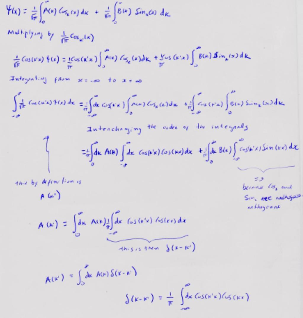
20

21 5..D Spectral decomposition in complex variable: The Fourier Transform. In expression (8) above we have x= dk[ dk[ which can be expressed as, x= ( x )= dk dk dk Cos ( kx') ( x' ) dx' ] Cos(kx) Sin ( kx') ( x' ) dx' ] Sin(kx) { Cos ( x' ) k Cos ( k x) } ( x' ) dx' {Sin ( k x' ) Sin ( k x) } ( x' ) dx' {Cos ( k( x' x) )} ( x' ) dx' In the expression above one can identify an even function in the variable k, ( x )= dk[ Cos ( k( x' x) ) ( x' ) dx' ]() Even function in the variable k accordingly, we have the following equality dk [ Cos ( k( x' x) ) ( x' ) dx' ] dk [ Cos ( k( x' x) ) ( x' ) dx' ] (notice the different range of integration in each integral). ()

22 Thus, expression () can be re-written as, ( x )= dk [ On the other hand, notice the following identity, = - i dk [ Cos ( k( x' x) ) ( x' ) dx' ] (3) Sin ( k( x' x) ) ( x' ) dx' ] (4) where i is the complex number satisfying i = -. This follows from the fact that the function within the bracket is an odd function with respect to the variable k. From (3) and (4) we obtain ( x )= dk [Cos ( k( x' x) ) i Sin ( k( x' x) )] ( x' ) dx' ik( x' x) e (x) = ik( x' x) dk [e ] ( x' ) dx' (5) Rearranging the terms, ( x )= dk e ikx [e - ikx' ( x' ) dx' ] ( x )= [e - ikx' F(k) ( x' ) dx' ik x ]e dk ( x )= ik x F(k)e dk where F(k) = - ikx' e ( x' ) dx'

23 In summary, using the infinite and continuum basis-set of complex functions, BASIS-SET { e k, k } (6) where e k ( x ) e ikx an arbitrary function can be expressed as a linear combination of such basis-set functions, ( x )= F(k) e i k x dk Base-functions Fourier coefficients where the weight coefficients F(k) of the complex harmonic functions components are given by, (7) F(k) = e - i k x' ( x' ) dx' (8) which is typically referred to as the Fourier transform of the function. 5..E Correlation between localized-functions f = f(x) and spread- Fourier (spectral) transforms F = F(k) In essence, the Fourier formalism associates to a given function f its Fourier transform F. f F An important characteristic in the Fourier formalism is that, it turns out, the more localized is the function f, the broader its spectral Fourier transform F(k); and vice versa. (9) 3

24 f (x) F (k) Spatially localized pulse x corresponding Fourier spatial spectra k g (x) G(k) x Wider pulse narrower Fourier spectra Fig. 5.4 Reciprocity between a function and its spectral Fourier transform. k Due to its important application in quantum mechanics, this property (9) will be described in greater detail in the Section 5. below. It is worth to emphasize here, however, that the property expressed in (9) has nothing to do with quantum mechanics. It is rather an intrinsic property of the Fourier analysis of waves. However, later on when we identify (via the de Broglie hypothesis) some variables in the mathematical Fourier description of waves with corresponding physical variables characterizing a particle (i.e. position, linear momentum, etc), a better understanding of the quantum mechanical description of the world at the atomic level can be obtained. 5..F The Scalar Product in Complex Variable We will realize through the development of the coming chapters, that the quantum mechanics formalism requires the use of complex variables. Accordingly, let s extend the definition of scalar product to the case where the intervening functions are complex. Let Φ and ψ be two arbitrary complex functions. The scalar product between Φ and ψ is defined as follows, Φ ψ * Φ ( x) ψ( x) dx definition of scalar product. (3) 4

25 where the symbol * * then Φ = a i b.) stands for the complex conjugate. (For example, if Φ = a + i b Notice, that is, Φ ψ * * * * * * [ Φ ( x ) ψ( x) dx] [ Φ ( x) ψ( x) ] dx [ Φ( x) ψ ( x)] dx ; ψ * ψ (3) 5..G Notation using Bra-kets The description of some other common notations used in quantum mechanics books is in order. Particular case: Expansions in Fourier components Consider ( x )= F(k)e ik x dk. Notice that the corresponding Fourier-transform coefficient F(k) = ikx' e (x ) dx ' * (e ikx ) (x )dx can also be expressed in a more compact form (using the notation for scalar product) as ek (3) wheree k ( x ) e ikx Thus, if ( x )= F(k) e ik x dk which means = F(k) ek dk and we want to find the component F(k ), we simply multiply on the left by e k and obtain ek = F(k ) 5

26 It is also very common to, alternatively, express the wavefunction ( x ) in the brackets notation ψ equally represented by where all reference to the dependence on the spatial variable x is removed (or implicitly understood.) For example, a base function e ik x can be represented by a ket e k. Further, the ket e k is sometimes (if not often) simply denoted by k. (In the latter it is understood that the true meaning is the one given by the former.) More general case: Expansions in the base { ; n,,... The expression ( x ) = n A n n ( x ) }. n implies that the function is a linear combination of the base-functions { ; n,,...}. Thus, we can use the notation, n = n A n n or = n A n n (33) neither of which allude to the dependence on the spatial variable. This latter notation is very convenient since there are quantum systems whose wavefunction does not admit a spatial variable dependence (the spin, is a peculiar case.) For convenience (as we will see later in this course), it would be convenient to use the coefficient A n on the right side of ; n = n n A n (33) Another alternative notation of (33) is obtained by expressing A n in terms of the scalar product. In effect, since the basis is orthogonal and normalized basis n m mn then the expansion = n n A n implies 6

27 Accordingly, n = A n (34) = n n A n = n n n (35) 5. PHASE VELOCITY and GROUP VELOCITY Let s start with a simple example. Question: In the XYZ space, identify all the points (x,y,z) such that their vector position is perpendicular to the unit vector (,,). Answer: All the point on the plane YZ that passes through x= fulfills that requirement. Notice we can express the answer in an alternative way: all points r (x,y,z ) such that r (,,) fulfills that requirement. Question: How to express mathematically the set of points (x, y, z) located in the plane YZ that passes through the point 3(,, ). Answer: All points r (x,y,z ) such that r (,,) 3 fulfills that requirement. Question: Identify all points r (x,y,z ) such that r (,,) 7. Question: Identify all points r (x,y,z ) such that r (,,) 9. Question: Identify all points r (x,y,z ) such that r (,,) 4. Question: Identify all points r (x,y,z ) such that r (,,). Question: Identify all points r (x,y,z ) such that r (,,) A Planes Let r (x,y,z ) and nˆ be the spatial coordinates and a unit vector, respectively. Notice, r nˆ const locates the points r that constitute a plane oriented perpendicular to nˆ. 7

28 Different planes are obtained when using different values for the constant value (as seen in the figure below). Z X r n Y Z r c Side view Fig Left: A plane perpendicular to the unit vector nˆ. Right: Different planes are obtained when using different values for the constant value c in the expression r nˆ c( const ). c nˆ c 3 Y 5..B Traveling Plane Waves and Phase velocity Consider the two-variable vectorial function E of the form E ( r, t) E f ( rnˆ - vt o phase Function ) Constant vector where f is an arbitrary one-variable function and E o is a constant vector. For example, f could be the Cos function; i.e. E ( r, t) E cos( rnˆ - vt ) ) o 8

29 Notice, the points over a plane oriented perpendicular to nˆ and traveling with velocity v define the locus of points where the phase of the wave E remains constant. For this reason, the wave E ( r, t) E cos( rnˆ - vt ) is called a plane wave. o Z nˆ X Y Fig. 5.6 Schematic representation of a plane wave of electric fields. The figure shows the electric fields at two different planes, at a given instant of time. The fields lie oriented on the corresponding planes. The planes are perpendicular to the unit vector nˆ. Traveling Plane Waves (propagation in one dimension) f ( x vt) For any arbitrary function f, this represents a wave propagating to the right with speed v. f could be COS, EXP,... etc. f ( x vt ) phase Notice, a point x advancing at speed v will keep the phase of the wave f constant. For this reason v is called the phase velocity v ph. Traveling Harmonic Waves COS( kx t) COS [ k( x t) ] and k e i( k x t) These are specific examples of waves propagating to the right with phase velocity v ph = / k. In general ω ω(k). Note: The specific relationship ω ω(k) depends on the specific physical system under analysis (waves in a crystalline array of atoms, light propagation in a free space, 9

30 plasmons propagation at a metal-dielectric interface, etc.] ω ω (k) implies that, for different values of k, the corresponding waves travel with different phase velocities. 5..C A Traveling Wave-package and its Group Velocity Consider the expression f ( x) ( / ) F( k) e ikx dk as the representation of a pulse profile at t=. Here i( kx t) harmonic wave e at t. ikx e The profile of this pulse at a later time will be represented by, is the profile of the ψ i( k x t) ( x, t) dk e F( k) Pulse composed by a group of traveling harmonic waves (36) Since, each component e i( kx t) of the group travels with its own phase velocity, would still be possible to associate a unique velocity to the propagating group of waves? The answer is positive; it is called group velocity. Below we present an example that helps to illustrate this concept. Case: Wavepacket composed of two harmonic waves Analytical description) For simplicity, let s consider the case in which the packet of waves consists if only two waves of very similar wavelength and frequencies. ( x, t) Cos[ kxt] Cos[ ( k k) x ( ) t] (37) Using the identities Cos( A B) Cos( A) Cos( B) Sin( A) Sin( B) and Cos ( A B) Cos( A) Cos( B) Sin( A) Sin( B) one obtains Cos( A B) Cos( A B) Cos( A) Cos( B), which can be expressed as 3

31 Cos( A) Cos( A B A B B) Cos( ) Cos( ) Accordingly, (38) can be expressed as, ( x, t) Cos[ Since we are assuming that ( k ) x ( ) t ] Cos[ and k k ( k, we have k k ( x, t) Cos[ ( ) x ( ) t ] Cos[ kx t Modulation envelope ) x ( ] ) t (38) ] Notice, the modulation envelope travels with velocity equal to k which is known as the group velocity. v g, (39) In summary, k ( x, t) Cos[ ( ) x ( ) t ] Cos[ kx t Amplitude Modulating wave Planes, where the amplitude of the resultant wave remains constant, travel with speed ω V g k Carrier w a v e Plane of constant p h a s e traveling with speed ω V p k ] (4) The phase velocity is a measure of the velocity of the harmonic waves components that constitute the wave. The group velocity is the velocity with which, in particular, the profiles of maximum interference propagate. More general, the group velocity is the velocity at which the envelope profile propagate (as will be observed better in the graphic analysis given below). 3

32 Graphical description EXAMPLE-: Visualization of the addition of two waves whose k s and s are very similar in value. Case: Waves components of similar phase velocity, and group-velocity similar to the phase velocities. Let, C(z, t) = Cos [k z t] = Cos [ z t ] (4) D(z, t) = Cos [k z t] = Cos [. z t ] k = k =. =5 =.5 V= / k =.5 C D D C C= Cos( k z - w t ] D= Cos[ ( + z - ( t ] INDIVIDUAL WAVES At t=. E Region of constructive interference Region of constructive interference z Fig. 5.7a The profile of the individual waves C(z, t) and D(z, t) are plotted individually at t=. over the <z<75 range. 3

33 .5 k = k =. =5 =.5 V= / k =.5 At t=. ADDITION of WAVES C E C= Cos( k z - D= Cos[ ( +.5 D Regions of constructive interfere D C Region constructive i z Fig. 5.7b The profile of i) the individual waves C(z, t) and D(z, t) and ii) the profile of the sum C(z, t) + D(z, t), are plotted at t=. over the <z<75 range. The two plots given above are repeated once more but over a larger range in order to observe the multiple regions of constructive and destructive interference..5 k = =. w =5 =.5 V= / =.5 At t=. INDIVIDUAL WAVES C= Cos( k z - w t ] D= Cos[ ( + z - ( t ] E C D C Fig. 5.8a Regions of constructive interference z Regions of constructive interference 33

34 SUM at t=. Cos[.5(Dk)x-.5(Dw). ].5 At t=. ADDED WAVES C E C= Cos( k z - w t ] D= Cos[ ( + z - (.5 D Regions of constructive interference D C Regions of constructive interference z Fig. 5.8b The profile of the individual waves C(z, t) and D(z, t) given in expression (4) k = above, as well as the profile of the sum C(z, t) + D(z, t) are plotted at t=. over the <z<6 range w =5 =.5 V= / =.5 The total wave C(z,t) + D(z,t) (the individual waves C and D are given in expression (4) above) is plotted at different times in order to visuualize the net motion of the interference profiles (group velocity). k = k =. =5 =.5 V = / k =.5 phase V =k =.5 group C= Cos( k z - w t ] D= Cos[ (k +k) z - ( +t ] GROUP VELOCITY =.5 SUM at t=. SUM at t=4.4 C+D at t=. C+D at t=4 Cos[.5(Dk)x-.5(Dw). ] Cos[.5(Dk)x-.5(Dw)4 ]. SUM_at_t=._and_t=4_DATA -. Envelope profile at t= z x = t = 3.9 Envelope profile at t=4 Fig. 5.9 Notice, the net displacement of the valley is ~ units, which occurs during an incremental time of 4 -. =3.9 units. This indicates that the envelope profile travels with a velocity equal to / 3.9 ~.5. This value coincides with the value of k =.5/. 34

35 wave- (at t=.) wave-+wave- (at t=.) In the example above: The phase velocity of the individual waves are 5/=.5 and 5.5/.=.5 The group velocity as observed in the graph above is: /3.9 =.5 The group velocity as calculated from k is.5 EXAMPLE-: Visualization of the addition of two waves whose k s and s are very similar in value. Case: Waves components of similar phase velocity, but group-velocity different than the phase velocity. Let, C(z, t) = Cos [k z t] = Cos [ z t ] (4) D(z, t) = Cos [k z t] = Cos [. z t ].4.6 k = k =. =5 =. V = / k =.5 phase V =k= group C+D at t=. C= Cos( k z - w t ] D= Cos[ (k +k) z - ( +t ] GROUP VELOCITY = C+D at t=4 wave-+wave- (at t=. Envelope at t=.) Wave-+Wave-_at_t=4 Envelope-at t=4 wave- (at t=.) wave-(at t=.).8 Data Envelope profile at t=. Envelope profile at t= z 4 x = 4 t = 3.9 Fig. 5. Notice the net displacement of the valley of the envelope is approximately equal to 4, which divided by the incremental time (4-.=3.9), gives a velocity equal to 4/3.9 ~. This value coincides with / k =./. =. In the example above: The phase velocity k of the individual waves are 5/=.5 and 5./.=.4 respectively. 35

36 The group velocity as observed in the graph above is: The observed group velocity coincides with k is Comparing Fig. 5.9 and Fig. 5. we get evidence that the wavepackets of the first group velocity advances faster than the second group, despite the fact that the components have similar phase velocity. Phasor method to analyze a wavepacket It becomes clear from the analysis above that a packet composed of only two single harmonic waves of different wavelength can hardly represents a localized pulse. Rather, it represents a train of pulses. Below we show the method of phasors to add up multiple waves, which will help us understand, in a more simple way, how to represent a single pulse. First, let s try to understand qualitatively, from a phasors addition point of view, how a train of (multiple) pulses is formed. e i phasor Im Complex variable plane Cos( ) Real axis = kx-t e i(kx- phasor t) Im Complex variable plane (kx-t) Cos(kx-t) Real axis Fig. 5. A phasor representation in the complex plane. 36

37 Case: Let s consider the wave (x,t) = Cos (kx t) and analyze it at a given fixed time (t=. for example) Analysis using only real variable First we plot the profile of the wave at t= At t=. (x,t) = Cos( k x -.w ] 5 5 k= w=5 V=/ =.5 x C E C D Notice, as x changes the phase (kx w.) changes. Analysis using complex variable, phasors x e i( k x - ) phasor Im (kx.) =Cos(kx.) Complex variable plane Real axis Notice, as x changes the phase (kx w.) changes. Case: wavepacket composed of two waves Let s consider the addition of two harmonic waves (x,t) = Cos( k x -t) Cos( k x -t ) A phase phase where, without losing generality, we will assume k B k k. A B k k A B Real. Also, let s call (43) 37

38 To evaluate (43) we will work in the complex plane. Accordingly, to each wave we will associate a corresponding phasor, ~ (x,t) = e i( k A e x -t ) i( kbx-t ) Complex (44) On the right side, ach phasor component has magnitude equal to. (But below we will draw them as it they had slightly different magnitude just for clarity) The projection of the (complex) phasors along the horizontal axis will give the real-value (x,t) we are looking for in (43). Notice in (44) that, ~ (x,t) = [ i k Ax i kbx -it e e ] e Hence, we can analyze first only the factor [ factor -i t e later on. i k Ax i kb x e e ]. One can always add the ~ k x i k x (x) = [ i A B e e ] (45) Notice that at a given position x, the phase-difference between the two wave components is equal to, Phase difference k x k x (46) The following happens: B ( k k B A A ) x a) Real analysis for t= and different values of x According to (43), at x both waves have the same phase equal to zero. The waves then interfere constructively there. So x= is the first point of constructive interference. 38

39 .5 k = k =. =5 =.5 V= / k =.5 C D C D C= Cos( k z - w t ] Cos( k D= Cos[ ( + z - ( t A x) ] Cos( k B x) INDIVIDUAL WAVES At t= x - x = -.5 Region of Region of constructive interference constructive interference Constructive - Interference at this position z Complex (phasosr) analysis: Similarly, since the phase of each of the two waves in (45) is the same at x =, the corresponding phases will be aligned to each other (see figure below). Thus the amplitude of the total phasor, associated to x =, is maximum. Graphically, at t = and x = we will have, Im Im Real At x = At x = Real 39

40 At t > and x = we will have: Im t Real At x= Variation of the phases as time changes. Now, Let s keep the time fixed at t =. b) Variation of the phases as the position x changes As x increases a bit, the interference is not as perfect (amplitude is less than ) since the phase of the waves start to differentiate from each other; ( k k ) x Im Im B A. k B x Real k A x Real At x= At x Fig. 5. Analysis of wave addition by phasors in the complex plane. For clarity, the magnitude of one of the phasors has been drawn larger than the other one. Notice, once a value of x is chosen and left fixed, as the time advances all the phasors will rotate clockwise at angular velocity. k B x k A x k B x - k A x 4

41 c) As x increases, it will reach a particular value x x that makes the phase difference between the waves equal to. The value of x is determined by the condition, ( kb ka) x.that is, the waves interfere constructively again at x / k, where kb ka k. k B x k A x k B x k A x k B k A k At x x π/ Δk The phasors align again Fig. 5. Left: In general, at arbitrary value of x, the phasors do not coincide. Right: At a particular specific value x=x, both phasors coincide, thus giving a maximum value to the sum of the waves (at that location.) The phasors diagram also makes clear that as x keeps increasing, constructive interference will also occur at multiple values of x. It is kexpected = then k that =. the wave-pattern (the sum of the two waves) observed =5 =.5 around x will repeat again at around x x. V= / k =.5 INDIVIDUAL WAVES.5 C C= Cos( k z - w t ] Cos(k D B x) CCos(k D= A x) Cos[ ( + z - ( t ] D At t=. E x x = x=x Region of constructive interference z Region of constructive interference 4

42 Im k B x k A x Real At x o = At x x π/ Δk d) Notice that additional regions of constructive interference will occur at positions x satisfying ( k k ) x n x n B A n or x n n / k (n =,, 3, ) The phasors diagram, therefore, makes clear that as x keeps increasing, additional discrete values (x, x, x 3, etc) will be found to produce additional maxima. A(k) ( x )= Cos( k x) + Cos( k x) k k k k x x 3 x 4 x x Fig. 5.3 Wavepacket composed of two harmonic waves. Case: A wavepacket composed of several harmonic waves M When adding several harmonic waves Ai Cos( kix ), with M >, the condition for i having repeated regions of constructive interference still can occurs. In effect, First, there will be of course a constructive interference around x=. Second, we expect the existence of a position x=x that will make each of the quantities (k i -k j )x equal to a multiple of. (k i -k j ) x = (integer) ij (47) for all the ij combinations, with i and j =,, 3,, M. When this happens, it would mean that all the corresponding phasors coincide, thus giving a maximum of amplitude. 4

43 Third, additional regions of maximum interference will occur at multiple integers of x. A(k) k k x x x k o Fig. 5.4 Wavepacket composed of a large number of harmonic waves (to be compared with Fig. 5.3 above.) The train of pulses are more separated from each other. Notice also that, the greater the number M of harmonic components in the packet (with wavevectors k i within the same range k shown in the figure above), the more stringent becomes for all the M waves to satisfy at once the condition (47) for constructive interference. This means, a greater value of x may be needed any time an extra number of harmonic waves are included in the packet. Since the other maxima of interference occur at multiple values of x, we expect, therefore, that the greater number of k-values (within the same range k), the more separated from each other will be the regions of constructive interference. This is shown in Fig Case: Wavepacket composed of an infinite number of harmonic waves Adding more and more wavevectors k (still all of them within the same range k show in the figure below)) will make the value of x to become greater and greater. As we consider a continuum variation of k, the value of x will become infinite. That is, we will obtain just one pulse. A(k) k o k k x Fig. 5.5 Wavepacket composed of wavevectors k within a continuum range k produces a single pulse. x 43

44 What about the variation of the pulse-size as the number of wavevectors (all with values within the range k) increases? Fig. 5.5 above already suggests that the size should decrease. In effect, as the number of harmonic waves increases, the multiple addition of waves tends to average out to zero, unless x = or for values of x very small; that is the pulse becomes narrower. Thus, we now can understand better the property stated in a previous paragraphs above (see expression (9) above, where the properties of the Fourier transform were being discussed.) the more localized the function the broader its spectral response; and vice versa. In effect, notice in the previous figure that if we were to increase the range k, the corresponding range x of values of the x coordinate for which all the harmonic wave component can approximately interfere constructively would be reduced; and vice versa. A(k) k x k o k) x) A(k) k x k) (x) In short: 44

45 A wavepacket ( x )= x F(k)e ik x dk has the following property, k ~ (48) In the expression for the wavepacket, x is interpreted as the position coordinate and k as spatial-frequency. Mathematically, we can also express a temporal pulse as ( t )= A()e i t d, so also we expect the following relationship, ~ t (48) Expressions (48) and (48) are general properties of the Fourier analysis of waves. In principle, they have nothing to do with Quantum Mechanics. We will see later that one way to describe QM is within the framework of Fourier analysis. In this context, some of the mathematical terms ( and, to be more specific) are identified (via the de Broglie wave-particle duality hypothesis, to be expressed below) with the particle s physical variables (p and E). Once this is done, then p and E) become subjected to the relationship indicated in (48) and (48). The fact that physical variables are subjected to the relationships like in (48) and (48) constitute one of the cornerstones of Quantum Mechanics. We will explore this concept in the following section. 5.3 DESCRIBING the MOTION of a FREE PARTICLE in the context of the WAVE-PARTICLE DUALITY According to Louis de Broglie, a particle of linear momentum p and total energy E is associated with a wavelength an a frequency given by, h / p where is the wavelength of the wave associated with the particle s motion; and ν E/h the total energy E is related to the frequency ν of the wave associated with its motion. where h is the Planck s constant; h =6.6x -34 Js. 45

46 But the de Broglie postulate does not tell us how the waveparticle propagates. If, for example, the particle were to be subjected to forces, its momentum could change in a very complicate way, and potentially not a single wavelength would be associated to the particle (maybe many harmonic waves would be needed to localize the particle.) The de Broglie postulate does not allow predicting such dynamic response (the Schrodinger equation, to be introduced in subsequent chapters, does that.) As a first attempt to describe the propagation of a particle (through the space and time) lets consider first the simple case of a free particle (free particle motion implies that its momentum p and energy E remain constant.) Our task is to figure out the wavefunction that describes the motion of a free particle. 5.3.A Proposition-: Using a wavefunction with a definite linear momentum Taking into account the associated de Broglie s wavelength and frequency, let s construct (by making an arbitrary guess) a wavefunction of the form, ψ ( x,t ) ACos [ math π λ x t ] π ACos [ (px Et) ] h physics First attempt to describe a free-particle wave-function (49) Notice in (49) that a single value of linear momentum (that is p) characterizes this function. This (guessed) wavefunction (49) is proposed following an analogy to the description of electromagnetic waves, π ε ( x, t) ε o Cos [ x νt] electric field wave (5) λ where, as we know, the intensity I (energy per unit time crossing a unit cross-section area perpendicular to the direction of radiation propagation) is proportional to ε ( x, t). Let s check whether or not the proposed wavefunction (46) is compatible with our classical observations of a free particle motion. 46

47 For example, if our particle were moving with a classical velocity v classical, would we get the same value (somehow) from the wavefunction (x,t) (49)? given in First, notice for example that the wavefunction (49) has a phase velocity given by, v E p (phase velocity) (5) wavefuncti on / On the other hand, let s calculate the value of E/p for a non-relativistic classical particle, which gives, From (5) and (5), one obtains, E m (vclassical ), and p m vclassical, E / p vc lassical (5) v wavefuncti on v classical (53) We realize here a disagreement between the velocity of the particle and the phase velocity of the wave-particle the particle. v classical v wavefunction that is supposed to represent This apparent shortcoming may be attributed to the fact that the proposed wavefunction (49) has a definite momentum p (and thus an infinite spatial extension). A better selection of a wavefunction has to be made then in order to describe a particle more localized in space. That is explored in the next section. 5.3.B Proposition-: Using a wave-packet as a wave-function Let s assume our classical particle of mass m is moving with velocity vclassical v o classical velocity (54) (or approximately equal to v o ). Let s build a wavefunction in terms of the value To represent this particle, let s build a Fourier wave-packet such that, v o i) Its dominant harmonic component is one with wavelength λ h/ mv, or o o 47

48 wavenumber or, equivalently, in terms of the variable p, ii) Its dominant harmonic component has momentum k o / ( / h)mv (55) o o o o p p mv (56) That is, we would choose an amplitude A (p) that peaks when p is equal to the classical value of the particle s momentum. In the meantime, the width x and p of the wave packet are, otherwise, arbitrary. A(p) x) p o p p x x Accordingly, we start building a wave-packet of the form: ( x, t) ~ A Cos [ x νt] d Δλ In terms of the momentum variable π ( x, t) ~ A( p) Cos [ (px Et )] dp h Using the variables π Δp p h / λ and energy E/h where E E( p) p / m for we are considering a free no relativistic particle case. k p and ω E, (57) h π h and expressing the package rather with the complex variable, we propose k x ωt x t A k e i [( )] (, ) dk π ( ) (58) k Whose dominant harmonic component is k=k o given in (55,) k / ( / h)mv ). o o o 48

49 The group velocity of this wave-packet is given by, need to find an expression for as a function of k. v wavefunction's group-vellocity dω dk ko. Therefore we CASE: For a non-relativistic free particle Using (57), we obtain, ω( k ) π h E π h p m h π k m The group velocity of the wave-packet is given by, v Using (57), v wavefuncti group-vellocity on's dω dk p E. m dω h ko (59) dk m wave- function' s group-vellocity ko ko po m v o (6) Comparing this expression with expression (54), we realize that the wavepacket (58) represents better the non-relativistic particle, since the classical velocity is recovered through the group-velocity of the wavefunction. The multiple-frequency wave-packet (58), instead of the single frequency expression (49,) represents better the particle since, at least for the moment, its groupvelocity coincides with classical velocity of the particle. Consequences: THE PARAGRAPH BELOW IS VERY IMPORTANT! Notice, if a wave-packet (composed of harmonic waves with momentum-values p within a given range p) is going to represent a particle, then, according to the Fourier analysis there will be a corresponding extension x (wavepacket spatial width), which could be interpreted as the particle s position. That is, there will not be a definite exact position to be associated with the particle, but rather a range of possible values (within x.) In short, there will be an uncertainty in the particle s position. In addition, if the Fourier analysis is providing the right tool to make connections between the wave-mechanics and the expected classical results (for example, allowing us to identify the classical velocity with the wave-packet s group velocity) then we should be bounded by the other consequences inherent in the Fourier analysis. One of 49

50 them, for example, is that x ~ (see statement (9) and expression (48) and (48) k above), which has profound consequences in our view of the mechanics governing Nature. Indeed, from (53) k p ; thus x ~ x ~ implies h k p, where p h we have defined h/. x ~ /p implies that the better we know the momentum of the particle (that is, the narrower the range p in the wavepacket), the larger uncertainty x to locate the particle. This is quite an unusual result to classical mechanics, where we are used to specify the initial conditions of a particle s motion by giving the initial position and initial velocity simultaneously with limitless accuracy. That is, we are used to have x and p specified as narrow as we want (we assume there was nothing wrong with it.) By contrary, in the world where the dual wave-particle reins, we have to live with the constrains that (55) implies: we can not improve the accuracy in knowing x without scarifying the accuracy of p, and vice versa. In the next chapter we will further familiarize with this new quantum behavior. (55) Summary: In this chapter we tried to figure out a wavefunction to describe the free motion of the particle. According to Louis de Broglie, a particle of linear momentum p and total energy E is associated with a wavelength an a frequency given by, h / p where is the wavelength of the wave associated with the particle s motion; and ν E/h the total energy E is related to the frequency ν of the wave associated with its motion. where h is the Planck s constant; h =6.6x -34 Js. π We found that associating the particle with a wave ε ( x, t) ε o Cos [ x νt] of λ single spatial frequency k= and single temporal frequency, leads to an unacceptable result. Here and k (or p and E) are related through E=p /m in the case of a non-relativistic free particle. 5

51 A wavepacket ( x, t) ~ A( p) Cos [ ( px Et)] dp of width k and (and through h Δp the relation E=p /m ) width E was then postulated to represent a particle. The wavepacket would have a main component at p=p classical. When calculating the group velocity of the wavepacket at p=p classical it turns out to be equal to the classical velocity. That is, the classical particle and the wavepacket travel at the same speed). Here we follow closely Quantum Physics, Eisberg and Resnick, Section 3. 5