AEA Continuing Education Program. Machine Learning and Econometrics. Susan Athey, Stanford Univ. Guido Imbens, Stanford Univ.

Transcription

1 AEA Continuing Education Program Machine Learning and Econometrics Susan Athey, Stanford Univ. Guido Imbens, Stanford Univ. January 7-9, 2018

2 Machine Learning for Economics: An Introduction SUSAN ATHEY (STANFORD GSB)

3 Two Types of Machine Learning SUPERVISED Independent observations Stable environment Regression/prediction: E[Y X=x] Classification Pr(Y=y X=x) UNSUPERVISED Collections of units characterized by features Images Documents Individual internet activity history Find groups of similar items

4 Classification Advances in ML dramatically improve quality of image classification

5 Classification X i Neural nets figure out what features of image are important Features can be used to classify images i Relies on stability

6 What s New About ML? Flexible, rich, datadriven models Increase in personalization and precision Methods to avoid overfitting

7 Ability to Fit Complex Shapes

8 Prediction in a Stable Environment Goal: estimate and minimize MSE in a new dataset where only X is observed MSE: No matter how complex the model, the output, the prediction, is a single number Can hold out a test set and evaluate the performance of a model Ground truth is observed in a test set Only assumptions required: independent observations, and joint distribution of (Y,X) same in test set as in training set Note: minimizing MSE entails bias variance tradeoff, and always accept some bias Idea: if estimator too sensitive to current dataset, then procedure will be variable across datasets Models are very rich, and overfitting is a real concern, so approaches to control overfit necessary Idea of ML algorithms Consider a family of models Use the data to select among the models or choose tuning parameters Common approach: cross validation Break data into 10 folds Estimate on 9/10 of data, estimate MSE on last tenth, for each of a grid of tuning parameters Choose the parameters that minimize MSE ML works well because you can accurately evaluate performance without add l assumptions Your robotic research assistant then tests many models to see what performs best

9 What We Say v. What We Do (ML) What we say ML = Data Science, statistics Is there anything else? Use language of answering questions or solving problems, e.g. advertising allocation, salesperson prioritization Aesthetic: human analyst does not have to make any choices All that matters is prediction What we do Use predictive models and ignore other considerations E.g. Causality, equilibrium or feedback effects Wonder/worry about interpretability/reliability/robustne ss/ adaptability, but have little way to ask algos to optimize for it

10 Contrast with Traditional Econometrics Economists have focused on the case with substantially more observations than covariates (N>>P) In sample MSE is a good approximation to out of sample MSE OLS is BLUE, and if overfitting is not a problem, then no need to incur bias OLS uses all the data and minimizes insample MSE OLS obviously fails due to overfitting when P~N and fails entirely when P>N ML methods generally work when P>N Economists worry about estimating causal effects and identification Causal effects Counterfactual predictions Separating correlation from causality Standard errors Structural models incorporating behavioral assns Identification problems can not be evaluated using a hold out set If joint dist n of observable same in training and test, will get the same results in both Causal methods sacrifice goodness of fit to focus only on variation in data that identifies parameters of interest

11 What We Say v. What We Do (Econometrics) What We Say Causal inference and counterfactuals God gave us the model We report estimated causal effects and appropriate standard errors Plus a few additional specifications for robustness What we do Run OLS or IV regressions Try a lot of functional forms Report standard errors as if we ran only one model Have research assistants run hundreds of regressions and pick a few representative ones Use complex structural models Make a lot of assumptions without a great way to test them

12 Key Lessons for Econometrics Many problems can be decomposed into predictive and causal parts Can use off the shelf ML for predictive parts Data driven model selection Tailored to econometric goals Focus on parameters of interest Define correct criterion for model Use data driven model selection where performance can be evaluated While retaining ability to do inference ML Inspired Approaches for Robustness Validation ML always has a test set Econometrics can consider alternatives Ruiz, Athey and Blei (2017) evaluate on days with unusual prices Athey, Blei, Donnelly and Ruiz (2017) evaluate change in purchases before and after price changes Tech firm applications have many A/B tests and algorithm changes Other computational approaches for structural models Stochastic gradient descent Variational Inference (Bayesian models) See Sendhil Mullainathan et al (JEP, AER) for key lessons about prediction in economics See also Athey (Science, 2017)

13 Empirical Economics in Five Years: My Predictions Regularization/data driven model selection will be the standard for economic models Prediction problems better appreciated Measurement using ML techniques an important subfield Textual analysis standard (already many examples) Models will explicitly distinguish causal parts and predictive parts Reduced emphasis on sampling variation Model robustness emphasized on equal footing with standard errors Models with lots of latent variables

14 An Introduction to Regularized Regression Machine Learning and Causal Inference Susan Athey Thanks to Sendhil Mullainathan for sharing slides

15 What we do in Econometrics: The Case of Regression Specify a model: Data set has observations i=1,..,n Use OLS regression on the entire dataset to construct an estimate Discuss assumptions under which some components of have a causal interpretation Consider that S n (set of observed units, i=1,..,n) is a random sample from a much larger population. Construct confidence intervals and test the hypothesis that some components are equal to zero. Theorem: OLS is BLUE (Best Linear Unbiased Estimator) Best = lowest-variance

16 Goals of Prediction and Estimation Goal of estimation: unbiasedness Goal of prediction: loss minimization, E.g. l, Use the data to pick a function that does well on a new data point

17 Key assumptions in both cases Stationary data generating process Estimation: Interested in a parameter of that process Prediction: Interested in predicting y

18 High v. Low Dimensional Analysis We have discussed prediction as a high dimensional construct Practically that is where it is useful But to understand how high dimensional prediction works we must unpack an implicit presumption Presumption: Our known estimation strategies would be great predictors if they were feasible

19 A Simple OLS example Suppose we truly live in a linear world Write x = (1,x)

20 OLS seems like a good predictor Especially since it is known to be efficient

21 An Even Simpler Set-up Let s get even lower dimensional No variables at all Suppose you get the data of the type: You would like to estimate the mean

22 Forming an estimator of the mean Minimize bias: The sample mean is an unbiased estimator Also what you would get from OLS regression on a constant

23 A prediction problem In the same setup, you are given n data points You would like to guess the value of a new data point from the same distribution Goal: minimize quadratic loss of prediction

24 Best Predictor

25 The higher alpha the lower the bias The higher alpha the more variable across samples it is

26 Key problem The unbiased estimator has a nice property: But getting that property means large sample to sample variation of estimator This sample to sample variation means that in any particular finite sample I m paying the cost of being off on all my predictions

27 Intuition I see your first test score. What should my prediction of your next test be? Your first test score is an unbiased estimator But it is very variable Note: Bayesian intuition Even simpler: what was my guess before I saw any information Shrink to that In this example I m shrinking to zero

28 But in a way you know this As empiricists you already have this intuition

29 Back to Simple OLS example Suppose we truly live in a linear world Write x = (1,x)

30 A Simple Example You run a one variable regression and get Would you use the OLS coefficients to predict Or drop the first variable and use this:

31 Deciding whether to drop Suppose in the (impossible) case we got the true world right. (0,2) are the right coefficients Of course OLS does perfectly (by assumption). But how would OLS do on new samples where (0,2) being the generating coefficients? We re giving OLS a huge leg up here.

32 OLS Performance

33 What if we dropped the variable

34 Your standard error worry!

35 Where does your standard error intuition come from? You see a standard error You think that variable is not significant so you might not want to include it. But this is misleading

36

37

38

39

40 Your Standard Error Worry For hypothesis testing se tells you whether the coefficient is significant are not For prediction it s telling you how variable an estimator using it really is

41 Dual purposes of the standard eror The standard error also tells you that even if you re right on average: Your estimator will produce a lot of variance And then in those cases you make systematic prediction mistakes. Bias variance tradeoff Being right on average on the coefficient is not equal to the best predictor.

42 The Problem Here Prediction quality suffers from: Biased coefficients Variability in estimated coefficients Even if the true coefficient is 2, in any sample, we will estimate something else OLS is lexicographic First ensure unbiased Amongst unbiased estimators: seek efficiency Good predictions must trade these off

43 Two Variable Example Belaboring the point here Assume now that we have two variables As before, both normally distributed unit variance Your estimator produces

44 What would you do now? Logic above suggests you would drop both variables? Or keep both variables? It really depends on how you feel about the variance (10)?

45 Calculation

46 Hidden in Bias-Variance Tradeoff Covariance is central The standard error on several variables can be large, even though together their effect is highly consistent For prediction covariance between x matters

47 In a way this problem is not important The variance term diminishes with sample size Prediction-estimation wedge falls off as But variance term increases with variables Prediction-estimation rises with k So this is a problem when Function class high dimensional relative to data

48 What this means practically In some cases what you already know (estimation) is perfectly fine for prediction This is why ML textbooks teach OLS, etc. They are perfectly useful for the kinds of prediction problems ML tries to solve in low dimensional settings But in high dimensional settings Note: high dimensional does not ONLY mean lots of variables! It can mean rich interactions.

49 So far All this gives you a flavor of how the prediction task is not mechanically a consequence of the estimation task But it doesn t really tell you how to predict Bias variance tradeoff is entirely unactionable What s the bias? What s the variance? This is not really a tradeoff you can make A different look at the same problem produces a practical insight though

50 Back to OLS AVERAGES NOTATION: for sample ave. for sample The real problem here is minimizing the wrong thing: In-sample fit vs out-of-sample fit

51 Overfit problem OLS looks good with the sample you have It s the best you can do on this sample Bias-variance improving predictive power is about improving out of sample predictive power Problem is OLS by construction overfits We overfit in estimation

52 This problem is exactly why wide data is troubling Similarly think of the wide data case Why are we worried about having so many variables? We ll fit very well (perfectly if k > n) in sample But arbitrarily badly out of sample

53 Understanding overfit Let s consider a general class of algorithms

54 A General Class of Algorithms Let l,, for some loss function l (e.g., squared error) Note: L is an unknown function: we don t know P Consider algorithms of the form, argmin is used here as shorthand for sample mean observations in sample of size n OLS is an empirical loss minimizer: it minimizes the sample average over observed data of the loss function So empirical loss minimization algorithms are defined by the function class they choose from For estimation what we typically do Show that empirical loss minimizers generate unbiasedness

55 Empirical Loss minimization Leads to unbiasedness/consistency Fit the data you have In a frequentist world on average (across all S n ) this will produce the right thing This is usually how we prove consistency/unbiasedness Other variants: MLE

56 Some Notation Define The best we can do The best in the subset of functions that the algorithm looks at Recall: L is infeasible b/c we don t know true datagenerating process Contrast the latter with:, What the in-sample loss minimizer actually produces given a sample

57 Performance of Algorithm Performance of a predictor Performance of an Algorithm Algorithm s expected loss (Suppress S n in some of the notation for estimator)

58 The performance of A Understanding estimation error: Wrong function looks good in-sample Algorithm does not see this

59 Basic Tradeoff These two terms go hand in hand:

60 Approximation Overfit Tradeoff If we reduce set of f to reduce possible over-fit: Then we fit fewer true functions and drive up Only way to avoid this is if we knew information about f* so we could shrink the set

61 Unobserved overfit So the problem of prediction really is managing unobserved overfit We do well in-sample. But some of that fit is overfit.

62 Return to the original example Greater Chance To Overfit Less Chance To Overfit We drove down overfit by doing a constrained optimization

63 Basic Tradeoff at the Heart of Machine Learning Bigger function classes The more likely we are to get to the truth (less approximation) The more likely we are to overfit So we want to not just minimize in-sample error given a class of functions We also want to decide on the class of functions More expressive means less approximation error More expressive means more overfit

64 Let s do the same thing here Unconstrained, But we are worried about So why not do this instead? s.t. Complexity measure: tendency to overfit

65 Return to the original example Greater Overfit Better approximation Less Overfit Worse approximation More Expressive R(f) higher Less Expressive R(f) lower Reduce overfit by approximating worse Choose less expressive function class

66 Constrained minimization We could do a constrained minimization But notice that this is equivalent to:, Complexity measure should capture tendency to overfit

67 Basic insight Data has signal and noise More expressive function classes- Allow us to pick up more of the signal But also pick up more of the noise So the problem of prediction becomes the problem of choosing expressiveness

68 Overall Structure Create a regularizer that: Measures expressiveness Penalize algorithm for choosing more expressive functions Tuning parameter lambda Let it weigh this penalty against in-sample fit

69 Linear Example Linear function class Regularized linear regression

70 Regularizers for Linear Functions Linear functions more expressive if use more variables Can transform coefficients

71 Computationally More Tractable Lasso Ridge

72 What makes a good regularizer? You might think Bayesian assumptions Example: Ridge A good regularizer can build in beliefs Those are great and useful when available But central force is tendency to overfit Example: Even if true world were not sparse or priors were not normal you d still do this

73 Summary Regularization is one half of the secret sauce Gives a single-dimensional way of deciding of capturing expressiveness, Still missing ingredient is lambda

74 Choosing lambda How much should we penalize expressiveness? How do you make the over-fit approximation tradeoff? The tuning problem. Use cross-validation

75 How Does Cross Validation Work? CV-Tuning CV-Training Train Tune Tuning Set = 1/5 of Training Set

76 Cross-Validation Mechanics Loop over cross-validation samples Train a deep tree on CV-training subset Loop over penalty parameters Loop over cross-validation samples Prune the tree according to penalty Calculate new MSE of tree Average (over c-v samples) the MSE for this penalty Choose the penalty that gives the best average MSE

77 LASSO c-v Example

78 Creating Out-of-Sample In Sample Major point: Not many assumptions Don t need to know true model. Don t need to know much about algorithm Minor but important point To get asymptotics right we need to make some regularity assumptions Side point (to which we return) We d like to choose best algorithm for sample size n But this will not do that. Why?

79 Why does this work? 1. Not just because we can split a sample and call it out of sample It s because the thing we are optimizing is observable (easily estimable)

80 This is more than a trick It illustrates what separates prediction from estimation: I can t observe my prior. Whether the world is truly drawn from a linear model But prediction quality is observable Put simply: Validity of predictions are measurable Validity of coefficient estimators require structural knowledge This is the essential ingredient to prediction: Prediction quality is an empirical quantity not a theoretical guarantee

81 Why does this work? 1. It s because the thing we are optimizing is observable 2. By focusing on prediction quality we have reduced dimensionality

82 To understand this Suppose you tried to use this to choose coefficients Ask which set of coefficients worked well out-of sample. Does this work? Problem 1: Estimation quality is unobservable Need the same assumptions as algorithm to know whether you work out of sample If you just go by fit you are ceding to say you want best predicting model Problem 2: No dimensionality reduction. You ve got as many coefficients as before to search over

83

84 Bayesian Interpretation of Ridge

85 Bayesian Interpretation of Ridge

86 Bayesian Interpretation of Ridge

87 POST-Lasso Important distinction: Use LASSO to choose variables Use OLS on these variables How should we think about these?

88

89

90 Soft Thresholding Why not Hard Thresholding? ˆ LASSO ˆ OLS SJL [3]1

91 Slide 77 SJL [3]1 \hat{\beta}_{ols}? Spiess, Jann Lorenz, 8/28/2015

92 Orthonormal: ˆ RIDGE ˆ OLS 1 ˆ RIDGE ˆ OLS SJL [2]

93 Slide 78 SJL [2]1 \hat{\beta}_{ols}? Spiess, Jann Lorenz, 8/28/2015

94 Can be very misleading

95 Coefficient on Number of Bedrooms

96 Coefficient on Number of Bedrooms

97 What is this about? Coefficient on Number of Bedrooms

98 Coefficient on Number of Bedrooms What is this about?

99

100 Prediction Policy Susan Athey-Machine Learning and Causal Inference Thanks to Sendhil Mullainathan for sharing his slides

101 Three Direct Uses of Prediction 1. Policy 2. Testing Whether Theories are Right 3. Testing Theory Completeness

102 When is Prediction Primary Focus? Economics: allocation of scarce resources An allocation is a decision. Generally, optimizing decisions requires knowing the counterfactual payoffs from alternative decisions. Hence: intense focus on causal inference in applied economics Examples where prediction plays the dominant role in a decision Decision is obvious given an unknown state Many decisions hinge on a prediction of a future state

103 Prediction and Decision-Making: Predicting a State Variable Kleinberg, Ludwig, Mullainathan, and Obermeyer (2015) Motivating examples: Will it rain? (Should I take an umbrella?) Which teacher is best? (Hiring, promotion) Unemployment spell length? (Savings) Risk of violation of regulation (Health inspections) Riskiest youth (Targeting interventions) Creditworthiness (Granting loans) Empirical applications: Will defendant show up for court? (Should we grant bail?) Will patient die within the year? (Should we replace joints?)

104 Allocation of Inspections Examples: Auditors Health inspectors Fire code inspectors Equipment Efficient use of resources: Inspect highest-risk units (Assuming you can remedy problem at equal cost for all )

105

106 Prediction Problem Over 750,000 joint replacements every year Benefits Improved mobility and reduced pain Costs Monetary: $15,000 (roughly) Non-monetary: short-run utility costs as people recover from surgery

107 Look at death rate in a year How well are we doing avoiding unnecessary surgery? Medicare claims data 2010 surgeries for joint replacement Average death rate is 5% But is that the right metric for excess joint replacements? Don t want average patient Want marginal patient Predictably highest risk patients

108 Approach: use ML methods to predict mortality as a function of covariates e.g. regularized regression, random forest Put individuals into percentiles of mortality risk A large number of joint replacements going to people who die within the year Could we just eliminate the ones above a certain risk?

109 Econometrics of Prediction Policy Problems 1. Problem: Omitted Payoff Bias

110 This Unobservable is a Problem What if those with high Mortality also benefit most? Pain

111 Omitted Payoff Bias Y f (X, Z) g(x 0,W ) ) Cov(X, Z) is not a problem Cov(X,W ) is a problem

112 Econometrics of Prediction Policy Problems 1. Omitted Payoff Bias Like omitted variable bias but not in y Can partially assess on the basis of observables

113 No sign of bias: Highest risk show no signs of greater benefit

114 Quantifying gain of predicting better Allocation problem: Reallocate joints to other eligible patients How to estimate the risk of those who didn t get surgery? Look at those who could get surgery but didn t Doctors should choose the least risky first So those who don t receive should be particularly risky. Take a conservative approach Compare to median risk in this pool

115

116 Assessing the Research Agenda Follows economic tradition of using data to improve policy In an area of economic interest Similar to a lot of health econ work Of course this does not answer all questions of interest Why not?

117 Another Prediction Policy Problem Each year police make over 12 million arrests Many detained in jail before trial Release vs. detain high stakes Pre-trial detention spells avg. 2-3 months (can be up to 9-12 months) Nearly 750,000 people in jails in US Consequential for jobs, families as well as crime Kleinberg Lakkaraju Leskovec Ludwig and Mullainathan

118 Judge s Problem Judge must decide whether to release or not (bail) Defendant when out on bail can behave badly: Fail to appear at case Commit a crime The judge is making a prediction

119 PREDICTION

120 Omitted Payoff Bias? Bail carefully chosen Unlike other sentencing no other concerns: Retributive justice Family & other considerations low Bad use case: Parole Decision

121 Evaluating the Prediction NOT just AUC or Loss Use predictions to create a release rule What is the release crime rate tradeoff? Note: There s a problem

122 Econometrics of Prediction Policy 1. Omitted Payoff Bias 2. Selective Labels Problems What do we do with people algorithm releases that judge jails? (Like people who get surgery and didn t before)

123

124 Selective Labels Revisted What is the crime rate we must use? For released defendants, empirical crime rate For jailed ones, imputed crime rate But imputation may be biased Judge sees factors we don t Suppose young people have dots on their foreheads Perfectly predictive: judge releases only if no dot In released sample: young people have no crime We would falsely conclude young people have no risk. But this is because the young people with dots are in jail. We would then falsely presume when we release all young people we will do better than judge Key problem: unobserved factors seen by judge affect crime rate (& judge uses these wisely) How to fix?

125 Is not problem when we look just at released 55% Key insight: Contraction Would judges knowingly release at 55% risk? Willing to live with very high crime rates? Or Judges mispredicting

126 Contraction Multiple judges with similar caseloads and different lenience Strategy: use most lenient judges. Take their released population and ask which of those would you incarcerate to become less lenient Compare to less lenient judges

127 Jailed Jailed Released Jail Released 90% Judge Contraction 90% Judge Jailed Released Imputation

128 Impute Jailed Measure Released Imputation 80% Judge Peformance 90% Judge Measure Contraction

129 Contraction Requires Judges have similar cases (random assignment) Does not require judges having similar rankings But does give performance of a different rule Human constrained release rule

130 Contraction and Imputation Compared

131 Selective Labels In this case does not appear to be a problem But generically a problem Extremely common problem occurs whenever prediction -> decision -> treatment Data generated by previous decisions

132

133

134

135 Econometrics of Prediction Policy Problems 1. Omitted Payoff Bias 2. Selective Labels 3. Restricted Inputs

136 Restricted Inputs Race and gender are not legal to use We do not use them But is that enough? Reconstruction problem Optimizing in presence of this additional reconstruction constraint Rethinking disparate impact and disparate treatment

137 Racist Algorithms?

138 Econometrics of Prediction Policy Problems 1. Omitted Payoff Bias 2. Selective Labels 3. Restricted Inputs 4. Response to Decision Rule

139 Comparing Judges to Themselves

140 Why do we beat judges? Judges see more than we do Perhaps that is the problem Suggests behavioral economics of salience important here In general, any kind of noise

141 General points here Need more ways of comparing human and machine predictions Notion of private information called into question

142 Summary Many prediction policy problems Raise their own econometric challenges Can also provide conceptual insights

143 Causal Inference for Average Treatment Effects Professor Susan Athey Stanford University Machine Learning and Causal Inference Spring 2017

144 The potential outcomes framework For a set of i.i.d. subjects i = 1,..., n, we observe a tuple (X i, Y i, W i ), comprised of A feature vector X i R p, A response Y i R, and A treatment assignment W i {0, 1}. Following the potential outcomes framework (Holland, 1986, Imbens and Rubin, 2015, Rosenbaum and Rubin, 1983, Rubin, 1974), we posit the existence of quantities Y (0) i and Y (1) i. These correspond to the response we would have measured given that the i-th subject received treatment (W i = 1) or no treatment (W i = 0). NB: We only get to see Y i = Y (W i ) i

145 The potential outcomes framework For a set of i.i.d. subjects i = 1,..., n, we observe a tuple (X i, Y i, W i ), comprised of A feature vector X i R p, A response Y i R, and A treatment assignment W i {0, 1}. Define the average treatment effect (ATE), the average treatment effect on the treated (ATT) [ τ = τ ATE = E Y (1) Y (0)] [ ; τ ATT = E Y (1) Y (0) ] W i = 1 ; and, the conditional average treatment effect (CATE) [ τ (x) = E Y (1) Y (0) ] X = x.

146 The potential outcomes framework

147 The potential outcomes framework If we make no further assumptions, it is not possible to estimate ATE, ATT, CATE, and related quantities. This is a failure of identification (infinite sample size), not a small sample issue. Unobserved confounders correlated with both the treatment and the outcome make it impossible to separate correlation from causality. One way out is to assume that we have measured enough features to achieve unconfoundedness (Rosenbaum and Rubin, 1983) { } Y (0) i, Y (1) i Wi X i. When this assumption + OVERLAP (e(x) (0, 1)) holds, causal effects are identified and can be estimated.

148 Identification E Yi (1) [ (1)] [ [ (1) Y i = EXi EY (1) i X Y i i = E Xi [ E Yi (1) X i [ = E Xi [ E Yi X i [ W i Pr(W i = 1 X i ) Y (1) i Y i W i Pr(W i = 1 X i ) [ Y i W ] i = E Yi Pr(W i = 1 X i ) ]] Xi ]] X i ]] Xi Argument is analogous for E [ Y 0], which leads to ATE; and similar arguments allow you to identify CATE as well as the counterfactual effect of any policy assigning units to treatments on the basis of covariates. This result suggests a natural estimator: propensity score weighting using the sample analog of the last equation.

149 The role of overlap Note that we need e(x) (0, 1) to be able to calculate treatment effects for all x. Intuitively, how could you possibly infer [Y (0) X i = x] if e(x) = 1? Note that for discrete x, the variance of ATE is infinite when e(x) = 0. Moving the goalposts : Crump, Hotz, Imbens, Miller (2009) analyze trimming, which entails dropping observations where e(x) is too extreme. Typical approaches entail dropping bottom and top 5% or 10%. Approaches that don t directly require propensity score weighting may seem to avoid the need for this, but important to understand role of extrapolation.

150 Propensity Score Plots: Assessing Overlap The causal inference literature has developed a variety of conventions, broadly referred to as supplementary analysis, for assessing credibility of empirical studies. One of the most prevalent conventions is to plot the propensity scores of treated and control groups to assess overlap. Idea: for each q (0, 1), plot the fraction of observations in the treatment group with e(x) = q, and likewise for the control group. Even if there is overlap, when there are large imbalances, this is a sign that it may be difficult to get an accurate estimate of the treatment effect.

151 Propensity Score Plots: Assessing Overlap Example: Athey, Levin and Seira analysis of timber. Assignment to first price or open ascending: in ID, randomized for subset of tracts with different probabilities in different geographies; in CA, small v. large sales (with cutoffs varying by geography). So W = 1 if auction is sealed, and X represents geography, size and year.

152 Propensity Score Plots: Assessing Overlap in ID Very few observations with extreme propensity scores

153 Propensity Score Plots: Assessing Overlap in CA Untrimmed v. trimmed so that e(x) [.025,.975]

154 Variance of Estimator: Discrete Case Suppose small number of realizations of X i. Under unconfoundedness, can analyze these as separate experiments and average up the results. How does conditioning on X i affect variance of estimator?

155 Variance of Estimator: Discrete Case Let Ê denote the sample average, V be the variance, π(x) be the proportion of observations with X i = x, and let e(x) be the propensity score (Pr(W i = 1 X i = x)). V(ˆτ(x)) = V( ˆ ATE) = x V ( Ê i:xi =x,w i =1(Y i ) ) = = x σ 2 (x) n π(x) e(x) σ 2 (x) n π(x) e(x) + σ 2 (x) n π(x) (1 e(x)). [ n(x) n σ 2 (x) n(x) e(x) + σ 2 (x) ]. n(x) (1 e(x)) σ 2 (x) [ 1 n e(x) + 1 ]. (1 e(x))

156 Estimation Methods The following methods are efficient when the number of covariates is fixed: Propensity score weighting Direct model of the outcome (model of E [ Y i Xi, W i ] ), e.g. using regression Propensity-score weighted regression of Y on X, W (doubly robust) The choice among these methods is widely studied: Other popular methods include matching, propensity score matching, propensity score blocking, which are not efficient but often do better in practice. Note: Hirano, Imbens, Ridder (2003) establish that more efficient to weight by estimated propensity score than actual.

157 Regression Case Suppose that conditional mean function is given by µ(w, x) = β (w) x. If we estimate using OLS, then we can estimate the ATE as ÂTE = X ( ˆβ (1) β ˆ(0) ) Note that OLS is unbiased and efficient, so the above quantity converges to the true values at rate n: X ( ˆβ (1) ˆβ (0) ) µ x (β (1) β (0) ) = O p ( 1 n )

158 High-Dimensional Analogs?? Obvious possibility: substitute in the lasso (or ridge, or elastic net) for OLS. But bias is a big problem. With lasso, for each component j: ˆβ (w) j β (w) j ( log(p) ) = O p n This adds up across all dimensions, so that we can only guarantee for the ATT: ( log(p) ) ÂTT ATT = O p X 1 X 0 β (0) 0 n

159 Imposing Sparsity: LASSO Crash Course Assume linear model, and that there are at most a fixed number k of non-zero coefficients: β 0 k. Suppose X satisfies a restricted eigenvalue condition: no small group of variables is nearly collinear. ( k log(p) ) ˆβ β 2 = O p n ˆβ log(p) ) β 1 = O p (k n With the de-biased lasso (post-lasso OLS) we can even build confidence intervals on ˆβ if k << n log(p). Applying to the ATT, where we need to estimate X 1 β (0) (the cf outcome for treated observations had they been control instead): ( ATT ˆ ATT = O p k X 1 X log(p) ) 0 n

160 Improving the Properties of ATE Estimation in High Dimensions: A Double-Selection Method Belloni, Chernozukov, and Hansen (2013) observe that causal inference is not an off-the-shelf prediction problem: confounders might be important if they have a large effect on outcomes OR a large effect on treatment assignment. They propose: Run LASSO of W on X. Select variables with non-zero coefficients at a selected λ (e.g. cross-validation). Run a LASSO of Y on X. Select variables with non-zero coefficients at a selected λ (may be different than first λ). Run a OLS of Y on W and the union of selected variables. (Not as good at purely predicting Y as using only second set.) Result: under approximate sparsity of BOTH propensity and outcome models, and constant treatment effects, estimated ATE is asymptotically normal and estimation is efficient. Intuition: with enough data, can find the variables relevant for bias. With approximate sparsity and constant treatment effect, there aren t too many, and OLS will be unbiased.

161 Single v. Double Selection in BCH Algorithm

162 More General Results Belloni, Chernozukov, Fernandez-Val and Hansen (2016) ( forthcoming Econometrica) have a variety of generalizations: Applies general approach to IV Allows for a continuum of outcome variables Observes that nuisance parameters can be estimated generally using ML methods without affecting the convergence rate, subject to orthoganality conditions Shows how to use a framework based on orthogonality in moment conditions

163 Doubly Robust Methods With small data, a doubly robust estimator (though not the typical one, where typically people use inverse propensity score weighted regression) is (with ˆγ i = 1 ê(x i ) ): ˆµ 0 1 = X 1 ˆβ (0) + Ê i:wi =0ˆγ i ( Yi X i ˆβ (0)) To see why, note that the term in parentheses goes to 0 if we estimate β (0) well, while to show that we get the right answer if we estimate the propensity score well, we rearrange the expression to be ˆµ 0 1 = ( X 1 Ê i:wi =0(ˆγ i X i ) ) ˆβ (0) + Ê i:wi =0ˆγ i Y i The first term has expectation 0, and the second term gives the relevant counterfactual, if the propensity score is well-estimated.

164 Doubly Robust Methods: A High-Dimensional Analog? ˆµ 0 1 = X 1 ˆβ (0) + Ê i:wi =0ˆγ i ( Yi X i ˆβ (0)) How does this relate to the truth? ˆµ 0 1 µ 0 1 = X 1 ( ˆβ (0) β (0) ) + Ê i:wi =0ˆγ i ( ɛi + X i β (0) X i ˆβ (0)) = ( X 1 ˆγ X 0 ) ( ˆβ (0) β (0) ) + Ê i:wi =0ˆγ i ɛ i With high dimensions, we could try to estimate ˆβ and the propensity score with LASSO or post-lasso rather than OLS. However, this may not be good enough. It is also not clear how to get good estimates of the inverse propensity score weights γ i, in particular if we don t want to assume that the propensity model is sparse (e.g. if the treatment assignment is a complicated function of confounders).

165 Residuals on Residuals Small data approach (a la Robinson s 1988) analyzed a semi-parametric model Model Yi = τw i + g(x i ) + ɛ i Goal: estimate τ Approach: residuals on residuals gives n-consistent and asymptotically normal estimator Regress Y i ĝ(x i ) on W i E[W i X i ]

166 Double Machine Learning Chernozhukov et al (2017): Model Yi = τw i + g(x i ) + ɛ i, E[W i X i ] = h(x i ) Goal: estimate τ Use a modern machine learning method like random forests to estimate the nuisance parameters Regress Y i ĝ(x i ) on W i E[W i X i ] 1 If ML method converges at the rate n 4, residuals on residuals gives n-consistent and asymptotically normal estimator

167 Comparing Straight Regression to Double ML Moments used in estimation: Regression: E[(Y i W i τ g(x i )) W i ] = 0 Double ML: E[((Y i ĝ(x i ) (W i ĥ(x i]))τ) (W i ĥ(x i))] = 0 Double robustness and orthogonality: Robinson s result implies that if ĝ(x i ) is consistent, then ˆτ is the regression coefficient of the residual on residual regression, and even if ĥ is wrong, the orthogonality of the residual of the outcome regression and the residual W i ĥ still holds Neyman orthogonality: the Double ML moment condition has the property that when evaluated at ĝ = g and ĥ = h, small changes in either of them do not change the moment condition. The moment condition is minimized at the truth. You are robust to small mistakes in estimation of nuisance parameters, unlike regression approach

168 Comparing Straight Regression to Double ML

169 An Efficient Approach with Non-Sparse Propensity The solution proposed in Athey, Imbens and Wager (2016) for attacking the gap ˆµ 0 1 µ 0 1 = ( X 1 ˆγ X 0 ) ( ˆβ (0) β (0) ) + Ê i:wi =0ˆγ i ɛ i is to bound 1st term by selecting γ i s using brute force. In particular: ˆγ = argmin γ ζ X 1 γ X 0 + (1 ζ) γ 2 2 The parameter ζ is a tuning parameter; the paper shows that ζ exists such that the γ s exist to tightly bound the first term above. With overlap, we can make X 1 γ log(p) X 0 be O( n ). Result: If the outcome model is sparse, estimate β using LASSO ) yielding bias of second term O p (k, so the bias term is O(k log(p) n log(p) n ), so for k small enough, the last term involving ˆγ i ɛ i dominates, and ATE estimator is O( 1 n ).

170 Why Approximately Balancing Beats Propensity Weighting One question is why the balancing weights perform better than the propensity score weights. To gain intution, suppose the propensity score has the following logistic form, e(x) = exp(x θ) 1 + exp(x θ). After normalization, the inverse propensity score weights satisfy γ i exp(x θ). The efficient estimator for θ is the maximum likelihood estimator, n ˆθ ml = arg max {W i X i θ ln(1 + exp(x i θ))}. θ i=1 An alternativeis the method of moments estimator ˆθ mm that balances the covariates exactly: X 0 = exp(x i θ) X i {j:w j =0} exp(x j θ). {i:w i =0}

171 Why Approximately Balancing Beats Propensity Weighting An alternative is the method of moments estimator ˆθ mm that balances the covariates exactly: X 0 = {i:w i =0} with implied weights γ i exp(x i ˆθ mm ). X i exp(x i θ) {j:w j =0} exp(x j θ). The only difference between the two sets of weights is that the parameter estimates ˆθ differ. The estimator ˆθ mm leads to weights that achieve exact balance on the covariates, in contrast to either the true value θ, or the maximum likelihood estimator ˆθ ml. The goal of balancing (leading to ˆθ mm ) is different from the goal of estimating the propensity score (for which ˆθ ml is optimal).

172 Summarizing the Approximate Residual Balancing Method of Athey, Imbens, Wager (2016) Estimate lasso (or elastic net) of Y on X in control group. Find approximately balancing weights that make the control group look like the treatment group in terms of covariates, while attending to the sum of squares of the weights. With many covariates, balance is not exact. Adjust the lasso prediction of the counterfactual outcome for the treatment group (if it had been control) using approximately balancing weights to take a weighted average of the residuals from the lasso model. Main result: if the model relating outcomes to covariates is sparse, and there is overlap, then this procedure achieves the semi-parametric efficiency bound. No other method is known to do this for non-sparse propensity models. Simulations show that it performs much better than alternatives when propensity is not sparse.

173 Simulation Experiment The design X is clustered. We study the following settings for β: Dense: β (1, 1/ 2,..., 1/ p), Harmonic: β (1/10, 1/11,..., 1/ (p + 9)), Moderately sparse: β (10,..., 10 }{{} 10, 1,..., 1 }{{} 90, 0,..., 0 }{{} p 100 ), Very sparse: β (1,..., 1 }{{} 10, 0,..., 0 }{{} p 10 ).

174 Simulation Experiment Beta Model dense harmonic moderately sparse very sparse Overlap (η) Naive Elastic Net Approximate Balance Approx. Resid. Balance Inverse Prop. Weight Inv. Prop. Resid. Weight Double-Select + OLS Simulation results, with n = 300 and p = 800. Approximate residual balancing estimates ˆβ using the elastic net. Inverse propensity residual weighting is like our method, except with γ i = 1/ê(X i ). We report root-mean-squared error for τ. Observation: Weighting regression residuals works better than weighting the original data; balanced weighting works better inverse-propensity weighting.

175 Simulation Experiment β j 1 ({j 10}) β j 1/j 2 β j 1/j n p η = 0.25 η = 0.1 η = 0.25 η = 0.1 η = 0.25 η = We report coverage of τ for 95% confidence intervals constructed by approximate residual balancing.

176 Simulation Experiment Treatment Effect Distr. of Treated Distr. of Controls We are in a misspecified linear model; the main effects model is 10-sparse and linear. X

177 Simulation Experiment n p Naive Elastic Net Approximate Balance Approx. Resid. Balance Inverse Prop. Weight Inv. Prop. Resid. Weight Double-Select + OLS Approximate residual balancing estimates ˆβ using the elastic net. Inverse propensity residual weighting is like our method, except with γ i = 1/ê(X i ). We report root-mean-squared error for τ 1.

178 Estimating the Effect of a Welfare-to-Work Program Data from the California GAIN Program, as in Hotz et al. (2006). Program separately randomized in: Riverside, Alameda, Los Angeles, San Diego. Outcome: mean earnings over next 3 years. We hide county information. Seek to compensate with p = 93 controls. Full dataset has n = Coverage Oracle Approx. Resid. Balance Double Select + OLS Lasso Resid. IPW No Correction n

179 Closing Thoughts What are the pros and cons of approximate residual balancing vs. inverse-propensity residual weighting? Pros of balancing: Works under weaker assumptions (only overlap). Algorithmic transparency.... Pros of propensity methods: Potential for double robustness. Potential for efficiency under heteroskedasticity. Generalizations beyond linearity....

180 An Introduction to Regression Trees (CART) Susan Athey, Stanford University Machine Learning and Causal Inference

181 What is the goal of prediction? Machine learning answer: Smallest mean-squared error in a test set Formally: Let be a test set. Think of this as a random draw of individuals from a population Let be a candidate (estimated) predictor MSE on test set is:

182 Regression Trees Simple method for prediction Partition data into subsets by covariates Predict using average within each subset Why are regression trees popular? Easy to understand and explain Businesses often need segments Software assigns different algorithms to different segments Can completely describe the algorithm and interpretation

183 Example: Who survived the Titantic?

184 Regression Trees for Prediction Data Outcomes Y i, attributes X i. Support of X i is X. Have training sample with independent obs. Want to predict on new sample Build a tree : Partition of X into leaves X j Predict Y conditional on realization of X in each region X j using the sample mean in that region Go through variables and leaves and decide whether and where to split leaves (creating a finer partition) using in-sample goodness of fit criterion Select tree complexity using crossvalidation based on prediction quality

185 Regression Trees for Prediction Outcome: Binary (Y in {0,1}) Two covariates Goal: Predict Y as a function of X Classify units as a function of X according to whether they are more likely to have Y=0 or Y=1

186 Regression Trees for Prediction (1) Tree-building: Use algorithm to partition data according to covariates (adaptive: do this based on the difference in mean outcomes in different potential leaves.) (II) Estimation/prediction: calculate mean outcomes in each leaf (III) Use cross-validation to select tree complexity penalty

187 Tree Building Details Impossible to search over all possible partitions, so use a greedy algorithm Do until all leaves have less than 2*minsize obs: For each leaf: For each observed value of each covariate : Consider splitting the leaf into two children according to whether Make new predictions in each candidate child according to sample mean Calculate the improvement in fit (MSE) Select the covariate j and the cutoff value that lead to the greatest improvement in MSE; split the leaf into two child leaves Observations In-sample MSE always improves with additional splits What is MSE when each leaf has one observation?

188 Problem: Tree has been over-fitted Suppose we fit a tree and pick a particular leaf. Do we expect that if we drew a new sample, we would get the same answer? More formally: Let be training dataset and be an independent test set Let l l, Is l?

189 What are tradeoffs in tree depth? First: note that in-sample MSE doesn t guide you It always increases with depth Tradeoff as you grow tree deeper More personalized predictions More biased estimates

190 Regression Trees for Prediction: Components 1. Model and Estimation A. Model type: Tree structure B. Estimator : sample mean of Y i within leaf C. Set of candidate estimators C: correspond to different specifications of how tree is split 2. Criterion function (for fixed tuning parameter ) A. In-sample Goodness-of-fit function: Q is = -MSE (Mean Squared Error)=- A. Structure and use of criterion i. Criterion: Q crit = Q is x # leaves ii. Select member of set of candidate estimators that maximizes Q crit, given 3. Cross-validation approach A. Approach: Cross-validation on grid of tuning parameters. Select tuning parameter with highest Out-of-sample Goodness-of-Fit Q os. B. Out-of-sample Goodness-of-fit function: Q os = -MSE

191 How Does Cross Validation Work? CV-Tuning CV-Training Train Tune Tuning Set = 1/5 of Training Set

192 Cross-Validation Mechanics Loop over cross-validation samples Train a deep tree on CV-training subset Loop over penalty parameters Loop over cross-validation samples Prune the tree according to penalty Calculate new MSE of tree Average (over c-v samples) the MSE for this penalty Choose the penalty that gives the best average MSE

193 Choosing the penalty parameter

194 Some example code

195

196 Pruning Code

197 A Basic Policy Problem Every transfer program in the world must determine Who is eligible for the transfer Typical goal of redistributive programs Transfer to neediest But identifying the neediest is easier said than done Thanks to Sendhil Mullainathan for providing this worked out example.

198 Typical Poverty Scorecard

199

200 Can we do better? This component of targeting is a pure prediction problem We fundamentally care about getting best predictive accuracy Let s use this example to illustrate the mechanics of prediction

201 Brazilian Data The data: 44,787 data points 53 variables Not very wide? Median Annual consumption (in dollars): monthly income 6 percent below 1.90 poverty line 14 percent below the 3.10 poverty line

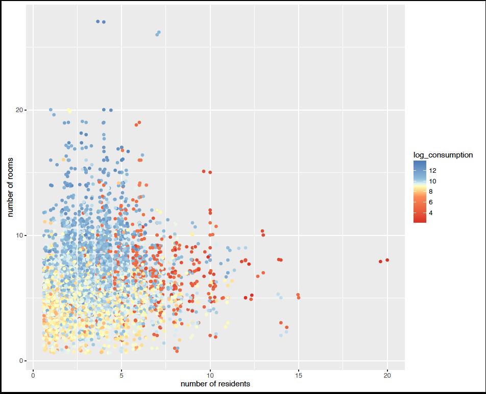
202 Consumption

203 log (consumption)

204 50 th Percentile

205 25 th Percentile

206 10 th Percentile

207

208

209

210

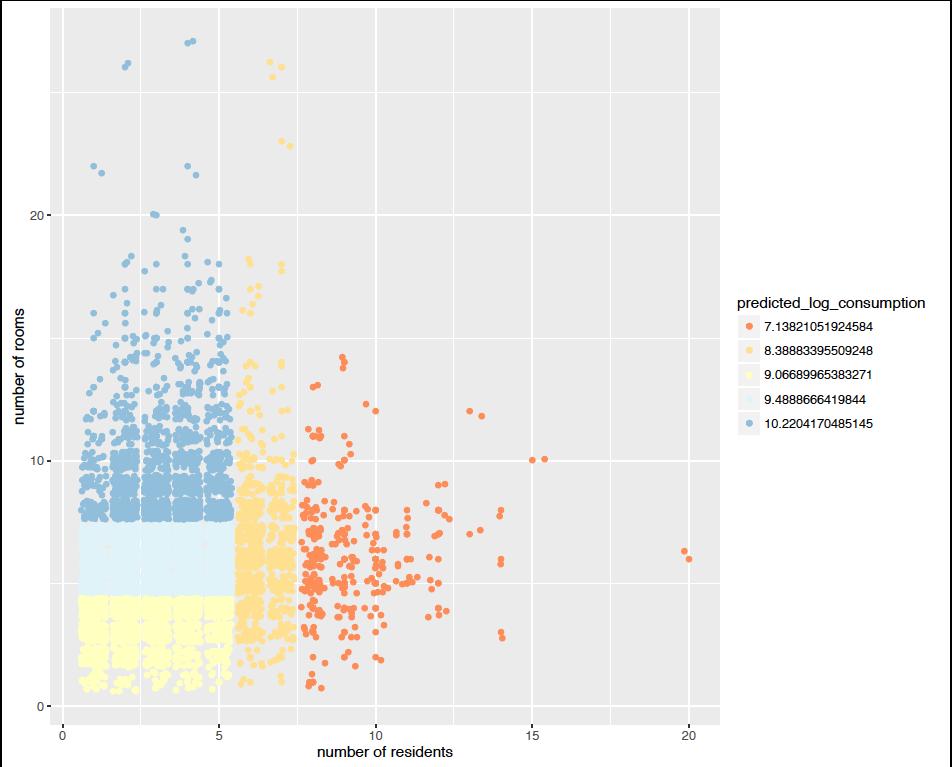
211 Two Variable Tree

212

213

214 28,573 data points to Fit with Set of Trees Fit trees on 4/5 of the data Fit a tree for every level of split size

215 28,573 data points to Fit with Set of Trees Set of Trees Set of Trees Set of Trees Set of Trees REPEAT leaving each fold out

216 Overfit Dominates

217 Why are we tuning on number of splits?

218 Questions and Observations How do we choose holdout set size? How to choose the # of folds? What to tune on? (regularizer)

219 What are these standard errors?

220 Questions and Observations How do we choose holdout set size? How to choose the # of folds? What to tune on? (regularizer) Which tuning parameter to choose from crossvalidation?

221 Tuning Parameter Choice Minimum? One standard error rule (rule of thumb) Which direction?

222 Output Which of these many trees do we output? Even after choosing lambda we have as many trees as folds Estimate one tree on full data using chosen cut size Key point: Cross validation is just for choosing tuning parameter Just for deciding how complex a model to choose

223 Questions and Observations How do we choose holdout set size? How to choose the # of folds? What to tune on? (regularizer) Which tuning parameter to choose from crossvalidation? Is there a problem tuning on subsets and then outputting fitted value on full set?

224 Lets look at the predictions Notice something?

225 WHY?

226 What does the tree look like?

227

228 What else can we look at to get a sense of what the predictions are?

229 Variable Importance Empirical loss by noising up x minus Empirical loss

230 How to describe model Large discussion of interpretability Will return to this But one implication is that the prediction function itself becomes a new y variable to analyze. Is any of this stable? What would a confidence interval look like?

231 Questions and Observations How do we choose holdout set size? How to choose the # of folds? What to tune on? (regularizer) Which tuning parameter to choose from crossvalidation? Is there a problem tuning on subsets and then outputting fitted value on full set? What is stable/robust about the estimated function?

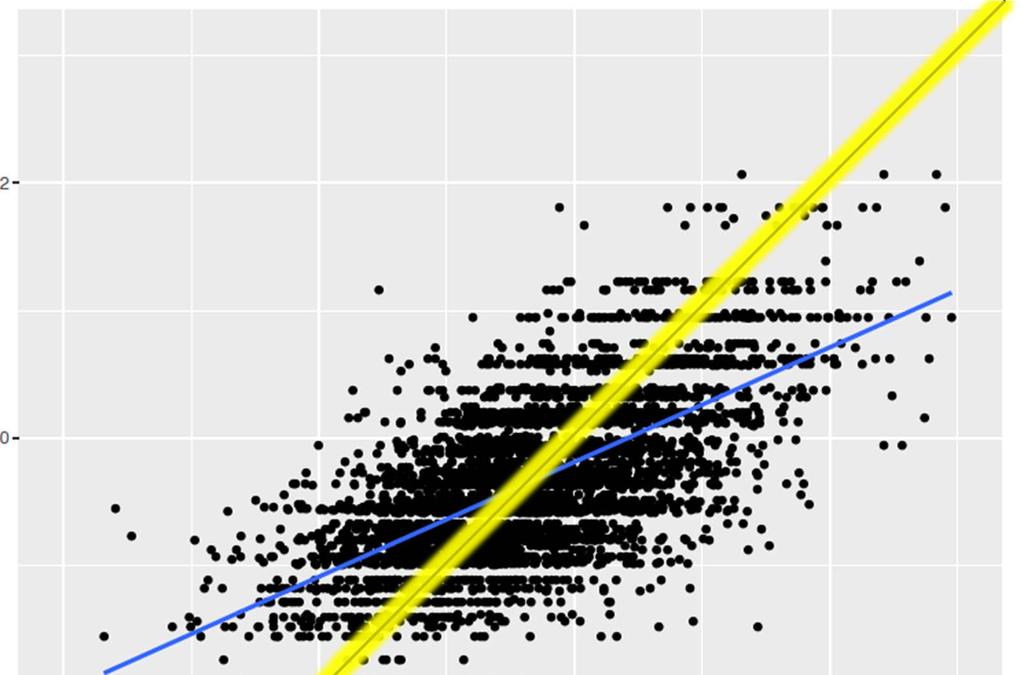
232 Measuring Performance

233

234 Measuring Performance Area Under Curve: Typical measure of performance What do you think of this measure?

235 What fraction of the poor do we reach?

236 Measuring Performance AUC: Typical measure of performance What do you think of this measure? Getting the domain specific meaningful performance measure Magnitudes Need point of comparison

237 What fraction of the poor do we reach? Confidence Intervals?

238 This is what we want from econometric theorems How do we choose holdout set size? How to choose the # of folds? What to tune on? (regularizer) Which tuning parameter to choose from crossvalidation? Is there a problem tuning on subsets and then outputting fitted value on full set? What is stable/robust about the estimated function? How do we form standard errors on performance?