Superintegrability and exactly solvable problems in classical and quantum mechanics

Transcription

1 Superintegrability and exactly solvable problems in classical and quantum mechanics Willard Miller Jr. University of Minnesota W. Miller (University of Minnesota) Superintegrability Penn State Talk 1 / 40

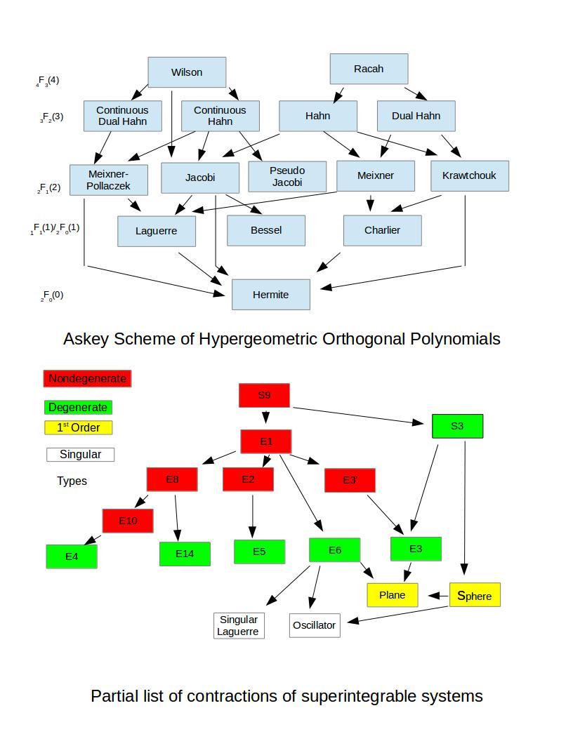
2 Abstract Quantum superintegrable systems are exactly solvable quantum eigenvalue problems. Their solvability is due to symmetry, but the symmetry is often hidden. The symmetry generators of nd order superintegrable systems in dimensions close under commutation to define quadratic algebras, a generalization of Lie algebras. The irreducible representations of these algebras yield important information about the eigenvalues and eigenspaces of the quantum systems. Distinct superintegrable systems and their quadratic algebras are related by geometric contractions, induced by generalized Inönü-Wigner Lie algebra contractions which have important physical and geometric implications, such as the Askey scheme for obtaining all hypergeometric orthogonal polynomials as limits of Racah/Wilson polynomials. We introduce the subject and and survey the theory behind the discovery and classification of these remarkable systems. W. Miller (University of Minnesota) Superintegrability Penn State Talk / 40

3 Outline 1 Introduction nd order systems 3 Constant curvature space Helmholtz systems 4 Interbasis expansion coefficients 5 Special functions and superintegrable systems 6 Higher order superintegrable systems 7 Wrap-up W. Miller (University of Minnesota) Superintegrability Penn State Talk 3 / 40

4 Introduction Superintegrable Systems We call a classical or quantum Hamiltonian system on an n-dimensional manifold n H = g ij p i p j + V (x i ), or H = n + V (x i ) i,j=0 (maximally, Nth-order) Superintegrable if it admits n 1 symmetry operators, i.e.,. {L i, H} = 0, [L i, H] = 0, i = 0,..., n 1, L 1 = H such that L,, L n 1 are polynomial, degree at most N, in the momenta or as differential operators. Superintegrable systems can be solved algebraically as well as analytically and are associated with special functions and exact solvability. W. Miller (University of Minnesota) Superintegrability Penn State Talk 4 / 40

5 Introduction Integrability and Superintegrability An integrable system has n algebraically independent symmetry operators in involution. A superintegrable system has n 1 algebraically independent symmetry operators (the maximum possible). The symmetries of a merely integrable system generate an abelian algebra, those of a superintegrable system generate an algebra that is necessarily nonabelian. Claim: Superintegrability captures what it means for a Hamiltonian system to be explicitly solvable. Some simple but important superintegrable systems: Kepler-Coulomb problem, the Hohmann transfer used in celestial navigation hydrogen atom: periodic table of the elements classical and quantum harmonic oscillator W. Miller (University of Minnesota) Superintegrability Penn State Talk 5 / 40

6 Introduction A very important but somewhat misleading example Newton used Kepler s laws to demonstrate that the equation governing the motion of a planet about the sun is m r = mk r ˆr, where r is the vector from the center of the sun to the center of the planet and ˆr is the unit vector in the direction of r. Here, M is the mass of the sun, m is the mass of the planet, k = MG and G is the gravitational constant. W. Miller (University of Minnesota) Superintegrability Penn State Talk 6 / 40

7 Introduction Newton s Gravitational force 1 We know today that Newton s equation for planetary motion, the -body problem, can be solved explicitly, not just numerically, because it is of maximal symmetry. It admits 3 independent symmetries and this is the maximum possible in two dimensions. It is a very important example of a superintegrable system. It also helps explain how Kepler found the trajectories of the planets without knowing Newton s equations or calculus. 3 A basic principle here is that symmetries of a physical system lead to conservation laws obeyed by the system: quantities that do not change as the system evolves in time. W. Miller (University of Minnesota) Superintegrability Penn State Talk 7 / 40

8 The orbital plane Introduction A planet orbiting the sun moves in a plane. Choose coordinates (x, y) in this plane such that the center of the sun is at the origin (0, 0) and at time t the center of the planet is at the point (x(t), y(t)) and is moving with velocity (ẋ(t), ẏ(t)). The speed of the planet in its orbit is s(t) = (ẋ(t)) + (ẏ(t)). W. Miller (University of Minnesota) Superintegrability Penn State Talk 8 / 40

9 Introduction Hamilton s equations 1 Let q 1, q be the position coordinates of a Hamiltonian system and let p 1, p be the momenta. The Hamiltonian function H(q 1, q, p 1, p ) represents the energy of the system. Hamilton s equations give the time evolution of the system. They are In our case, r = q k (t) = H pk, q 1 + q and ṗ k (t) = H qk, k = 1,. q 1 = x, q = y, p 1 = ẋ, p = ẏ, H = 1 (p 1 + p ) k r. Hamilton s equations are q 1 = ẋ, q = ẏ, ṗ 1 = ẍ = kx r 3, ṗ = ÿ = ky r 3, which are just Newton s equations for the -body problem. W. Miller (University of Minnesota) Superintegrability Penn State Talk 9 / 40

10 Hamilton s equations Introduction A function F (q 1, q, p 1, p ) is a symmetry or constant of the motion if F(q 1 (t), q (t), p 1 (t), p (t)) remains constant as the system evolves in time. Thus F is a constant of the motion if and only if From the chain rule, d dt F (q 1(t), q (t), p 1 (t), p (t)) = 0. d F F(t) = q 1 + F q + F p 1 + F p = dt q1 q p1 p F H + F H F H F H q1 p1 q p p1 q1 p q where {H, F } is the Poisson bracket of F and H. {H, F}, W. Miller (University of Minnesota) Superintegrability Penn State Talk 10 / 40

11 Introduction Hamilton s equations 3 Thus F is a constant of the motion provided the Poisson bracket {H, F } = 0. Note that H itself (the energy) is always a constant of the motion. In our case, in addition to the energy, we have the following constants of the motion: 1 Angular momentum L = q 1 p p 1 q. Proof: {H, L} = p p 1 p 1 p kq q 1 r 3 + kq q 1 r 3 = 0. W. Miller (University of Minnesota) Superintegrability Penn State Talk 11 / 40

12 Hamilton s equations 4 Introduction 1 The first component of the Laplace vector e 1 = p (q 1 p q p 1 ) kq 1. r The second component of the Laplace vector e = p 1 (q 1 p q p 1 ) kq. r are also constants of the motion. W. Miller (University of Minnesota) Superintegrability Penn State Talk 1 / 40

13 Introduction Constants of the motion Energy 1 ( (ẋ) + (ẏ) ) k x + y = E Angular momentum xẏ yẋ = L Laplace vector e = (e 1, e ) where ẏ(xẏ yẋ) kx x + y = e ky 1, ẋ(xẏ yẋ) x + y = e. Structure equations for symmetries: {L, e 1 } = e, {L, e } = e 1, {e 1, e } = LH Casimir: e 1 + e L H = k This is so(3) if H is constant. W. Miller (University of Minnesota) Superintegrability Penn State Talk 13 / 40

14 Introduction The trajectories 1 By lining up the x, y coordinate system so that the x-axis is in the direction of the Laplace vector, we can assume e = 0. (This means that the x-axis goes through the perihelion of the planet. It is called the apse axis in astronomy.) Then 1 ky e = 0 and L constant ẋ = L x + y e 1 and L constant ẏ = e 1 L + kx L x + y W. Miller (University of Minnesota) Superintegrability Penn State Talk 14 / 40

15 The trajectories Introduction 1 Substitute these expressions into the equation for L, and simplify to get the equation: k x + y = L e 1 x Square and simplify to get the trajectory (1 e 1 k )x + L e 1 k x + y = L4 k W. Miller (University of Minnesota) Superintegrability Penn State Talk 15 / 40

16 Introduction The paths are conic sections! Set e 1 = ɛk 0 where ɛ is called the eccentricity. ɛ = 0, Circle: 0 < ɛ < 1, Ellipse: ɛ > 1, Hyperbola: x + y = ( L k ) (1 ɛ )x + ɛl k x + y = ( L k ) (1 ɛ )x + ɛl k x + y = ( L k ) ɛl ɛ = 1, Parabola: k x + y = ( L k ) W. Miller (University of Minnesota) Superintegrability Penn State Talk 16 / 40

17 Nelson lecture 1 p.3/43 Impulse maneuvers 1. Position and velocity (x 0,y 0,x 0,y 0 ) at a single instant determines the trajectory: Just compute the constants of the motion E,L,e 1,e at the instant and they in term uniquely define the trajectory.. This is the basis for impulse maneuvers in rocket science. The Hohmann transfer.

18 Nelson lecture 1 p.4/43 The Hohmann transfer 1. Space ship (with engines turned off) on trajectory with constants of the motion E,L,e 1,e.. At time t 0 ship has position and velocity (x 0,y 0,x 0,y 0 ). 3. Turn on the engine, for an instant, at time t 0 : impulse propulsion. This pulse changes the velocity of the ship instantaneously, but not the position. 4. Immediately after the impulse the ship has position and velocity (x 0,y 0, x 0,ỹ 0 ). 5. This gives us the new trajectory with constants of the motion Ẽ, L,ẽ 1,ẽ. 6. The change of trajectories is determined by simple algebra.

19

20 Trajectory of Loiterer II P 3 4 A apse axis 0. First sighting 1. Second sighting. Hohmann transfer at periapsis 3. Elliptical orbit 4. Hohmann transfer at apoapsis 5. Geostationary orbit

21 Introduction The quantum Coulomb problem 1 The Hamiltonian and the the constants of the motion are replaced by differential operators: We make the formal replacement p 1 q1 and handle the ambiguity of replacements q i p i q i qi, qi q i by symmetrizing: q i p i 1 (q i qi + qi q i ). H = 1 ( q 1 + q ) k x + y L = q 1 q q q1, e 1 = 1 (L q + q L) e = 1 (L q 1 + q1 L) ky x + y kx x + y W. Miller (University of Minnesota) Superintegrability Penn State Talk 17 / 40

22 Introduction The quantum Coulomb problem The Poisson bracket {F, G} is replaced by the operator commutator [F, G] = FG GF and the constants of the motion are differential operators that commute with H. [H, L] = [H, e 1 ] = [H, e ] = [H, H] = 0. 1 Structure equations for symmetries: [L, e 1 ] = e, [L, e ] = e 1, [e 1, e ] = LH Casimir: e 1 + e L H + 1 H = k 3 Note that this is NOT a Lie algebra, unless H is a multiple of the identity operator. W. Miller (University of Minnesota) Superintegrability Penn State Talk 18 / 40

23 Introduction Transition to Quantum Mechanics 1 Bound states are eigenfunctions of H that are square integrable: HΨ = EΨ, < Ψ, Ψ >= 1. The symmetries commute with H, so they map the eigenspace into itself. We look for irreducible representations of the algebra generated by the symmetries. Necessarily, the Hamiltonian is the constant E in these cases, so we can consider the structure equations as defining so(3). 1 the possible states of energy E and angular momentum L have values E n = 4k (n + 1), L m = im/, m = n, n 1, n,, n so the possible multiplicities of the eigenvalues are n + 1 where n is an integer. These results can be derived entirely from the representation theory of so(3) (highest weight, lowest weight, etc.). W. Miller (University of Minnesota) Superintegrability Penn State Talk 19 / 40

24 Introduction The hydrogen atom on the -sphere 1 These striking results led to mathematical physicists to concentrate on finding systems with symmetries that generated Lie algebras. However, consider this analog analog of the hydrogen atom on the -sphere. H = 3 Ji αs 3 +, s1 + s i=1 where s 1 + s + s 3 = 1, J 1 = s 3 s 3 and J, J 3 by cyclic permutation. A basis for the symmetry operators is αs 1 L 1 = J 1 J 3 + J 3 J 1, L 1 = J 1 J 3 + J 3 J 1 s1 + s along with H. αs 1 s1 + s, X = J 3, W. Miller (University of Minnesota) Superintegrability Penn State Talk 0 / 40

25 Introduction The hydrogen atom on the -sphere The symmetry operators satisfy the structure relations [X, L 1 ] = L, [X, L ] = L 1, [L 1, L ] = 4HX 8X 3 + X, L 1 + L + 4X 4 4HX + H 5X α = 0. clearly not a Lie algebra. The irreducible representations of this algebra yield the energy eigenvalues with multiplicity n = 1. E n = 1 4 (n + 1) α (n + 1). (Studied by Schrödinger.) As the radius of the sphere goes to this system converges to the hydrogen atom system in D Euclidean space. W. Miller (University of Minnesota) Superintegrability Penn State Talk 1 / 40

26 Introduction Example: Smorodinski-Winternitz 1967 Generators: H = x + y ω (x + y ) + b 1 x + b y L 1 = x ω x + b 1 x, L = y ω y + b y, L 3 = (x y y x) + y b 1 x + x b y Structure relations: [R, L 1 ] = 8L 1 8HL 1 16ω L 3 + 8ω, [R, L 3 ] = 8HL 3 8{L 1, L 3 } + (16b 1 + 8)H 16(b 1 + b + 1)L 1, R {L 1, L 1, L 3 } 8H{L 1, L 3 } + (16b b )L 1 16ω L 3 (3b )HL 1 +(16b 1 + 1)H ω L ω (3b 1 + 3b + 4b 1 b + 3 ) = 0 The quantum Tremblay, Turbiner, Winternitz system (in polar coordinates in the plane) is Here, R [L 1, L ]. This is called a nondegenerate quadratic algebra. {A, B} AB + BA, and {A, B, C} are symmetrizers. W. Miller (University of Minnesota) Superintegrability Penn State Talk / 40

27 Introduction Example: Smorodinski-Winternitz 1967 Generators: H = x + y ω (x + y ) + b 1 x + b y L 1 = x ω x + b 1 x, L = y ω y + b y, L 3 = (x y y x) + y b 1 x + x b y Structure relations: [R, L 1 ] = 8L 1 8HL 1 16ω L 3 + 8ω, [R, L 3 ] = 8HL 3 8{L 1, L 3 } + (16b 1 + 8)H 16(b 1 + b + 1)L 1, R {L 1, L 1, L 3 } 8H{L 1, L 3 } + (16b b )L 1 16ω L 3 (3b )HL 1 +(16b 1 + 1)H ω L ω (3b 1 + 3b + 4b 1 b + 3 ) = 0 The quantum Tremblay, Turbiner, Winternitz system (in polar coordinates in the plane) is Here, R [L 1, L ]. This is called a nondegenerate quadratic algebra. {A, B} AB + BA, and {A, B, C} are symmetrizers. W. Miller (University of Minnesota) Superintegrability Penn State Talk / 40

28 nd order systems nd order superintegrable systems nd order systems are the easiest to construct and classify, due to their connection with separation of variables: every orthogonal separable coordinate system is characterized by n nd order symmetry operators, mutually commuting. All such superintegrable systems for nd order systems for D have been classified. There are 44 nondegenerate (3 parameter potential) systems, on a variety of manifolds, but under the Stäckel transform, an invertible structure preserving mapping, they divide into 6 equivalence classes with representatives on flat space and the -sphere. There are also a similar number of degenerate (1 parameter potential) systems that divide into 6 equivalence classes. All of these systems are multiseparable W. Miller (University of Minnesota) Superintegrability Penn State Talk 3 / 40

29 nd order systems nd order superintegrable systems nd order systems are the easiest to construct and classify, due to their connection with separation of variables: every orthogonal separable coordinate system is characterized by n nd order symmetry operators, mutually commuting. All such superintegrable systems for nd order systems for D have been classified. There are 44 nondegenerate (3 parameter potential) systems, on a variety of manifolds, but under the Stäckel transform, an invertible structure preserving mapping, they divide into 6 equivalence classes with representatives on flat space and the -sphere. There are also a similar number of degenerate (1 parameter potential) systems that divide into 6 equivalence classes. All of these systems are multiseparable W. Miller (University of Minnesota) Superintegrability Penn State Talk 3 / 40

30 nd order systems nd order superintegrable systems nd order systems are the easiest to construct and classify, due to their connection with separation of variables: every orthogonal separable coordinate system is characterized by n nd order symmetry operators, mutually commuting. All such superintegrable systems for nd order systems for D have been classified. There are 44 nondegenerate (3 parameter potential) systems, on a variety of manifolds, but under the Stäckel transform, an invertible structure preserving mapping, they divide into 6 equivalence classes with representatives on flat space and the -sphere. There are also a similar number of degenerate (1 parameter potential) systems that divide into 6 equivalence classes. All of these systems are multiseparable W. Miller (University of Minnesota) Superintegrability Penn State Talk 3 / 40

31 Constant curvature space Helmholtz systems Nondegenerate flat space systems: HΨ = ( x + y + V )Ψ = EΨ. 1 E1: V = α(x + y ) + β x + γ y, () E: V = α(4x + y ) + βx + γ y, 3 E3 : V = α(x + y ) + βx + γy, 4 E7: V = α(x+iy) + (x+iy) b (x+iy) b 5 E8 V = α(x iy) + β + γ(x + y ), (x+iy) 3 (x+iy) 6 E9: V = α + βy + γ(x+iy), x+iy x+iy β(x iy) ( x+iy+ (x+iy) b ) + γ(x + y ), 7 E10: V = α(x iy) + β(x + iy 3 (x iy) ) + γ(x + y 1 (x iy)3 ), 8 E11: V = α(x iy) + β(x iy) + γ, x+iy x+iy 9 E15: V = f (x iy), 10 1 E16: V = x (α + β +y 11 E17: V = α x +y + β (x+iy) + 13 E0: V = 1 x +y y+ x + γ +y y x ), +y γ (x+iy) x, +y β 1 E19: V = α(x+iy) + + γ. (x+iy) 4 ( (x iy)(x+iy+) (x iy)(x+iy ) α + β x + x + y + γ x x + y ), W. Miller (University of Minnesota) Superintegrability Penn State Talk 4 / 40

32 Constant curvature space Helmholtz systems Nondegenerate systems on the complex -sphere: HΨ = (J 3 + J 13 + J 1 + V )Ψ = EΨ, J kl = s k sl s l sk s 1 + s + s 3 = 1. Here, 1 S1: V = α (s 1 +is ) + βs 3 (s 1 +is ) + γ(1 4s 3 ) (s 1 +is ) 4, S: V = α β + s3 (s 1 +is + γ(s 1 is ) ) (s 1 +is, ) 3 3 α S4: V = (s 1 +is + βs ) 3 γ +, s 1 +s (s 1 +is ) s1 +s 4 S7: V = αs 3 + βs 1 + s 1 +s s γ, s 1 +s s 5 S8: V = αs + β(s +is 1 +s 3 ) + γ(s +is 1 s 3 ), s 1 +s3 (s +is 1 )(s 3 +is 1 ) (s +is 1 )(s 3 is 1 ) 6 S9: V = α s 1 + β s + γ, s3 W. Miller (University of Minnesota) Superintegrability Penn State Talk 5 / 40

33 Constant curvature space Helmholtz systems nd order systems with potential, K = The symmetry operators of each system close under commutation to generate a quadratic algebra, and the irreducible representations of this algebra determine the eigenvalues of H and their multiplicity All the nd order superintegrable systems are limiting cases of a single system: the generic 3-parameter potential on the -sphere, The coordinate limits are induced by generalized Inönü-Wigner Lie algebra contractions of the symmetry algebras of the manifolds underlying the superintegrable systems, either flat space or the complex sphere. These contractions have been classified. W. Miller (University of Minnesota) Superintegrability Penn State Talk 6 / 40

34 Constant curvature space Helmholtz systems nd order systems with potential, K = The symmetry operators of each system close under commutation to generate a quadratic algebra, and the irreducible representations of this algebra determine the eigenvalues of H and their multiplicity All the nd order superintegrable systems are limiting cases of a single system: the generic 3-parameter potential on the -sphere, The coordinate limits are induced by generalized Inönü-Wigner Lie algebra contractions of the symmetry algebras of the manifolds underlying the superintegrable systems, either flat space or the complex sphere. These contractions have been classified. W. Miller (University of Minnesota) Superintegrability Penn State Talk 6 / 40

35 Interbasis expansion coefficients S9: the generic system on the -sphere H = J1 + J + J3 + a 1 + a + a 3, a s1 s s3 j = 1 4 k j, where J 3 = s 1 s s s1 and J, J 3 are obtained by cyclic permutations of indices. Basis symmetries: (J 3 = s s1 s 1 s, ) L 1 = J 1 + a 3s s 3 + a s3, L s = J + a 1s3 s1 + a 3s1, L s3 3 = J3 + a s1 s + a 1s, s1 Structure equations: [L i, R] = 4{L i, L k } 4{L i, L j } (8 + 16a j )L j + (8 + 16a k )L k + 8(a j a k ), R = 8 3 {L 1, L, L 3 } (16a 1 + 1)L 1 (16a + 1)L (16a 3 + 1)L ({L 1, L }+{L, L 3 }+{L 3, L 1 })+ 1 3 (16+176a 1)L (16+176a )L (16+176a 3)L (a 1 + a + a 3 ) + 48(a 1 a + a a 3 + a 3 a 1 ) + 64a 1 a a 3, R = [L 1, L ]. W. Miller (University of Minnesota) Superintegrability Penn State Talk 7 / 40

36 Interbasis expansion coefficients S9: the generic system on the -sphere H = J1 + J + J3 + a 1 + a + a 3, a s1 s s3 j = 1 4 k j, where J 3 = s 1 s s s1 and J, J 3 are obtained by cyclic permutations of indices. Basis symmetries: (J 3 = s s1 s 1 s, ) L 1 = J 1 + a 3s s 3 + a s3, L s = J + a 1s3 s1 + a 3s1, L s3 3 = J3 + a s1 s + a 1s, s1 Structure equations: [L i, R] = 4{L i, L k } 4{L i, L j } (8 + 16a j )L j + (8 + 16a k )L k + 8(a j a k ), R = 8 3 {L 1, L, L 3 } (16a 1 + 1)L 1 (16a + 1)L (16a 3 + 1)L ({L 1, L }+{L, L 3 }+{L 3, L 1 })+ 1 3 (16+176a 1)L (16+176a )L (16+176a 3)L (a 1 + a + a 3 ) + 48(a 1 a + a a 3 + a 3 a 1 ) + 64a 1 a a 3, R = [L 1, L ]. W. Miller (University of Minnesota) Superintegrability Penn State Talk 7 / 40

37 Interbasis expansion coefficients ON basis of eigenfunctions of L 1, H: Ψ N n,n = (s1 + s) 1 (n+k 1+k +1) (1 s1 s) 1 (k 3+ 1 ) ( s1 + ) 1 (k + 1 ) ( s s1 + s s s 1 ) 1 (k 1+ 1 ) P (k,k 1 ) n ( s 1 s s1 + )P (n+k 1+k +1,k 3 ) s N n (1 s1 s), L 1 Ψ N n,n = (k 1 + k 1 (n k 1 + k ) Ψ N n,n, n = 0, 1,, N, HΨ N n,n = E N Ψ N n,n, E N = [N + k 1 + k + k 3 + ] + 1, N = 0, 1,. 4 Separable in spherical coordinates, orthogonal with respect to area measure on the 1st octant of the -sphere. Dimension of eigenspace E N is N + 1. P (α,β) n (y) = ( n + α n ) F 1 ( n α + β + n + 1 α + 1 These functions are defined even for n, N complex. ; 1 y ), Jacobi polynomials W. Miller (University of Minnesota) Superintegrability Penn State Talk 8 / 40

38 Interbasis expansion coefficients ON basis of eigenfunctions of L, H: Get immediately by permutation 1 3, n q, of L 1 basis: L Λ N q,q = (k 3 + k 1 (q k 3 + k ) Λ N q,q, q = 0, 1,, N, HΛ N q,q = E N Λ N q,q, E N = [N + k 1 + k + k 3 + ] + 1, N = 0, 1,. 4 Separable in a different set of spherical coordinates, orthogonal with respect to area measure on the 1st octant of the -sphere. Dimension of eigenspace E N is N + 1. W. Miller (University of Minnesota) Superintegrability Penn State Talk 9 / 40

39 Interbasis expansion coefficients Interbasis expansion coefficients 1 The action of L 1 on and L eigenbasis follows immediately from permutation symmetry. Now we expand the L eigenbasis in terms of the L 1 eigenbasis: N Λ N q,q = Rq n Ψ N n,n, n=0 q = 0,, N Applying L to both sides of this expression one can show that the expansion coefficients Rq n satisfy a 3-term recurrence relation in n with respect to multiplication by t = (q + k 1+k 3 +1 ), so the expansion coefficients are polynomials in t of order n. The action of the symmetry operators can be transferred to the expansion coefficients so that these polynomials form a basis for an irreducible representation of the quadratic symmetry algebra acting as difference operators on polynomials. W. Miller (University of Minnesota) Superintegrability Penn State Talk 30 / 40

40 Interbasis expansion coefficients The Wilson and Racah polynomials R n q 4 F 3 ( n, α + β + γ + δ + n 1, α t, α + t α + β, α + γ, α + δ ) ; 1 a polynomial in t. a j = 1 4 k j, k 1 = δ + β 1, k = α + γ 1, k 3 = α γ, N = α β, t = q + k 1 + k 3 + 1, The quadratic structure algebra of S9 can be identified with the Askey-Wilson algebra of these orthogonal polynomial. W. Miller (University of Minnesota) Superintegrability Penn State Talk 31 / 40

41 Special functions and superintegrable systems The big picture: Special functions Special functions arise in two distinct ways: As separable eigenfunctions of the quantum Hamiltonian. Second order superintegrable systems are multiseparable. As eigenfunctions in the model. Often solutions of difference equations. These are interbasis expansion coefficients relating distinct separable coordinate eigenbases. Most of the special functions in the DLMF appear in this way. W. Miller (University of Minnesota) Superintegrability Penn State Talk 3 / 40

42 Special functions and superintegrable systems The big picture: Special functions Special functions arise in two distinct ways: As separable eigenfunctions of the quantum Hamiltonian. Second order superintegrable systems are multiseparable. As eigenfunctions in the model. Often solutions of difference equations. These are interbasis expansion coefficients relating distinct separable coordinate eigenbases. Most of the special functions in the DLMF appear in this way. W. Miller (University of Minnesota) Superintegrability Penn State Talk 3 / 40

43 Special functions and superintegrable systems The big picture: Contractions and special functions Taking coordinate limits starting from quantum system S9 we can obtain other superintegrable systems. These limits induce limit relations between the special functions associated with the superintegrable systems. The limits induce contractions of the associated quadratic algebras, and via the models, limit relations between the associated special functions. For constant curvature systems the required limits are all induced by Wigner-type Lie algebra contractions of o(3, C) and e(, C)., The Askey scheme for orthogonal functions of hypergeometric type fits nicely into this picture. (Kalnins-Miller-Post, 014) Contractions have geometrical and physical significance: c, h 0, radius of sphere, etc. W. Miller (University of Minnesota) Superintegrability Penn State Talk 33 / 40

44 Special functions and superintegrable systems The big picture: Contractions and special functions Taking coordinate limits starting from quantum system S9 we can obtain other superintegrable systems. These limits induce limit relations between the special functions associated with the superintegrable systems. The limits induce contractions of the associated quadratic algebras, and via the models, limit relations between the associated special functions. For constant curvature systems the required limits are all induced by Wigner-type Lie algebra contractions of o(3, C) and e(, C)., The Askey scheme for orthogonal functions of hypergeometric type fits nicely into this picture. (Kalnins-Miller-Post, 014) Contractions have geometrical and physical significance: c, h 0, radius of sphere, etc. W. Miller (University of Minnesota) Superintegrability Penn State Talk 33 / 40

45 Special functions and superintegrable systems The big picture: Contractions and special functions Taking coordinate limits starting from quantum system S9 we can obtain other superintegrable systems. These limits induce limit relations between the special functions associated with the superintegrable systems. The limits induce contractions of the associated quadratic algebras, and via the models, limit relations between the associated special functions. For constant curvature systems the required limits are all induced by Wigner-type Lie algebra contractions of o(3, C) and e(, C)., The Askey scheme for orthogonal functions of hypergeometric type fits nicely into this picture. (Kalnins-Miller-Post, 014) Contractions have geometrical and physical significance: c, h 0, radius of sphere, etc. W. Miller (University of Minnesota) Superintegrability Penn State Talk 33 / 40

46 Special functions and superintegrable systems The big picture: Contractions and special functions Taking coordinate limits starting from quantum system S9 we can obtain other superintegrable systems. These limits induce limit relations between the special functions associated with the superintegrable systems. The limits induce contractions of the associated quadratic algebras, and via the models, limit relations between the associated special functions. For constant curvature systems the required limits are all induced by Wigner-type Lie algebra contractions of o(3, C) and e(, C)., The Askey scheme for orthogonal functions of hypergeometric type fits nicely into this picture. (Kalnins-Miller-Post, 014) Contractions have geometrical and physical significance: c, h 0, radius of sphere, etc. W. Miller (University of Minnesota) Superintegrability Penn State Talk 33 / 40

47 Special functions and superintegrable systems The big picture: Contractions and special functions Taking coordinate limits starting from quantum system S9 we can obtain other superintegrable systems. These limits induce limit relations between the special functions associated with the superintegrable systems. The limits induce contractions of the associated quadratic algebras, and via the models, limit relations between the associated special functions. For constant curvature systems the required limits are all induced by Wigner-type Lie algebra contractions of o(3, C) and e(, C)., The Askey scheme for orthogonal functions of hypergeometric type fits nicely into this picture. (Kalnins-Miller-Post, 014) Contractions have geometrical and physical significance: c, h 0, radius of sphere, etc. W. Miller (University of Minnesota) Superintegrability Penn State Talk 33 / 40

48

49

50 Model interplay Special functions and superintegrable systems W. Miller (University of Minnesota) Superintegrability Penn State Talk 36 / 40

51 The TTW System 1 Higher order superintegrable systems Before 009, relatively few examples of superintegrable systems of higher order than were known. This changed dramatically with the introduction of the TTW system, built on the Smorodinski Winternitz potential. The Smorodinski-Winternitz system in polar coordinates x = r cos θ, y = r sin θ is: H = r + 1 r r + 1 r θ ω r + 1 r ( α sin (θ) + β cos (θ) ) The Tremblay, Turbiner, Winternitz system (TTW, 009) is H = r + 1 r r + 1 r θ ω r + 1 r ( α sin (kθ) + β cos (kθ) ) where k = p q is rational. W. Miller (University of Minnesota) Superintegrability Penn State Talk 37 / 40

52 The TTW System 1 Higher order superintegrable systems Before 009, relatively few examples of superintegrable systems of higher order than were known. This changed dramatically with the introduction of the TTW system, built on the Smorodinski Winternitz potential. The Smorodinski-Winternitz system in polar coordinates x = r cos θ, y = r sin θ is: H = r + 1 r r + 1 r θ ω r + 1 r ( α sin (θ) + β cos (θ) ) The Tremblay, Turbiner, Winternitz system (TTW, 009) is H = r + 1 r r + 1 r θ ω r + 1 r ( α sin (kθ) + β cos (kθ) ) where k = p q is rational. W. Miller (University of Minnesota) Superintegrability Penn State Talk 37 / 40

53 The TTW System Higher order superintegrable systems For k = 1 this is the caged isotropic oscillator, for k = it is a Calogero system on the line, etc. TTW conjectured that this system was classically and quantum superintegrable for all rational k. Proved for the classical case by Kalnins, Pogosyan and Miller and in the quantum case by Kalnins, Kress and Miller (010). The 3rd constant of the motion is of arbitrarily high order. The algebra generated by the symmetries closes. Using this idea of obtaining higher order superintegrable systems from nd order systems, many families of higher order superintegrable systems have now been discovered and for some of them the structure of the symmetry algebras has been worked out. However, there is still no general theory of higher order systems. W. Miller (University of Minnesota) Superintegrability Penn State Talk 38 / 40

54 The TTW System Higher order superintegrable systems For k = 1 this is the caged isotropic oscillator, for k = it is a Calogero system on the line, etc. TTW conjectured that this system was classically and quantum superintegrable for all rational k. Proved for the classical case by Kalnins, Pogosyan and Miller and in the quantum case by Kalnins, Kress and Miller (010). The 3rd constant of the motion is of arbitrarily high order. The algebra generated by the symmetries closes. Using this idea of obtaining higher order superintegrable systems from nd order systems, many families of higher order superintegrable systems have now been discovered and for some of them the structure of the symmetry algebras has been worked out. However, there is still no general theory of higher order systems. W. Miller (University of Minnesota) Superintegrability Penn State Talk 38 / 40

55 The TTW System Higher order superintegrable systems For k = 1 this is the caged isotropic oscillator, for k = it is a Calogero system on the line, etc. TTW conjectured that this system was classically and quantum superintegrable for all rational k. Proved for the classical case by Kalnins, Pogosyan and Miller and in the quantum case by Kalnins, Kress and Miller (010). The 3rd constant of the motion is of arbitrarily high order. The algebra generated by the symmetries closes. Using this idea of obtaining higher order superintegrable systems from nd order systems, many families of higher order superintegrable systems have now been discovered and for some of them the structure of the symmetry algebras has been worked out. However, there is still no general theory of higher order systems. W. Miller (University of Minnesota) Superintegrability Penn State Talk 38 / 40

56 Wrap-up Wrap-up. 1 Superintegrable systems and their associated symmetry algebras are, essentially, those quantum and classical mechanical systems that can be solved exactly. These systems are related to one another by Stäckel transforms or (coupling constant metamorphosis) which preserve the symmetry algebra structure, and by contractions. Special functions are identified as functions that express solutions of solvable problems. Thus there are deep connections between the special functions of mathematical physics and superintegrable systems. For nd order systems, by taking contractions step-by-step from the S9 model we can recover the Askey Scheme. However, the contraction method is more general. It applies to all special functions that arise from the quantum systems via separation of variables, not just polynomials of hypergeometric type, and it extends to higher dimensions. W. Miller (University of Minnesota) Superintegrability Penn State Talk 39 / 40

57 Wrap-up Wrap-up. For nd order superintegrable systems there is a reasonably mature classification and structure theory and a large number of applications. For 3rd order systems there are some classification results. For higher order superintegrable systems there are many examples but, as yet, no classification and structure theory. W. Miller (University of Minnesota) Superintegrability Penn State Talk 40 / 40