MECHANICAL IMPEDANCE OF ANKLE AS A FUNCTION OF ELECTROMYOGRAPHY SIGNALS OF LOWER LEG MUSCLES USING ARTIFICIAL NEURAL NETWORK

Transcription

1 Michigan Technological University Digital Michigan Tech Dissertations, Master's Theses and Master's Reports - Open Dissertations, Master's Theses and Master's Reports 2015 MECHANICAL IMPEDANCE OF ANKLE AS A FUNCTION OF ELECTROMYOGRAPHY SIGNALS OF LOWER LEG MUSCLES USING ARTIFICIAL NEURAL NETWORK Chen JIA Michigan Technological University Copyright 2015 Chen JIA Recommended Citation JIA, Chen, "MECHANICAL IMPEDANCE OF ANKLE AS A FUNCTION OF ELECTROMYOGRAPHY SIGNALS OF LOWER LEG MUSCLES USING ARTIFICIAL NEURAL NETWORK", Master's Thesis, Michigan Technological University, Follow this and additional works at: Part of the Biomechanics and Biotransport Commons, and the Mechanical Engineering Commons

2 MECHANICAL IMPEDANCE OF ANKLE AS A FUNCTION OF ELECTROMYOGRAPHY SIGNALS OF LOWER LEG MUSCLES USING ARTIFICIAL NEURAL NETWORK By Chen JIA A THESIS Submitted in partial fulfillment of the requirements for the degree of MASTER OF SCIENCE In Mechanical Engineering MICHIGAN TECHNOLOGICAL UNIVERSITY Chen JIA

3

4 This thesis has been approved in partial fulfillment of the requirements for the Degree of MASTER OF SCIENCE in Mechanical Engineering Department of Mechanical Engineering-Engineering Mechanics Thesis Advisor: Mo Rastgaar Committee Member: Nina Mahmoudian Committee Member: Tomas B. Co Department Chair: William W. Predebon

5

6 Table of Contents Abstract... 7 Keywords... 7 I. Goals and Hypotheses... 7 II. Introduction... 8 III. Main Apparatus and Experiment Procedures A. Subjects B. Experimental Setup C. Experimental Protocol IV. Main Method A. Theory of Neural Network B. Function Fitting of Neural Network Toolbox V. Data Analysis and Modeling A. The Components of Collected Data B. Inputs of the ANN Model C. Outputs of the ANN Model D. Building ANN Model VI. Results of the Models and Discussions A. Regression B. Distribution of Errors C. Performance D. Tracking of Impedances in Frequency Domain VII. Conclusion and Future Works Acknowledgements References

7 Appendix A: Collected Data of All Ten Subjects...37 A. Regression R values...37 B. Distribution of Errors...38 C. Mean Squared Errors...40 D. Performance...41 Appendix B: Figures of All Single-Subject Based Models that Not Shown in the Paper...42 A. Regression Plots...42 B. Error Histogram...52 C. Performance Plots...58 D. Tracking of Impedances in Frequency Domain

8 Abtract--This paper reports on the feasibility of developing a model to describe the nonlinear relationship between the mechanical impedance of the human ankle within a specified range of frequency and the root mean square (RMS) value of the Electromyography (EMG) signals of the muscles of human ankle using Artificial Neural Network (ANN). A lower extremity rehabilitation robot Anklebot was used to apply pseudo-random mechanical perturbations to the ankle and measure the angular displacement of the ankle to estimate the data of ankle mechanical impedance. Meanwhile, the surface EMG signals from the selected muscles were monitored and recorded using a Delsys Trigno system. The final ANN models in this paper were created in two degrees of freedom dorsiflexion-plantarflexion (DP) and inversioneversion (IE) at 3 different muscle activation levels. The results of analysis of the ANN model showed the feasibility of developing models with adequate accuracy and to define the mechanical impedance of the human ankle in terms of lower extremity muscles EMG statistical properties. Keywords--Mechanical Impedance; Surface Electromyography (EMG) Signals; Human Ankle; Lower Leg Muscles; Multiple DoFs of Ankle Movement; Artificial Neural Network. I. Goals and Hypotheses: This paper reports on the feasibility of developing a model to describe the nonlinear relationship between the mechanical impedance of the human ankle within a range of frequency and the root mean square (RMS) value of the Electromyography (EMG) signals of the muscles of human ankle using Artificial Neural Network (ANN). In another word, models that accurately predict the mechanical impedance of ankle can be described by the following expression: f ( RMS, frequency) impedance The data for estimation of the ankle mechanical impedance was collected using a lower extremity rehabilitation robot, Anklebot. This therapeutic robot enables reliable characterization of the torque-angle relation at the ankle in two degrees of freedom simultaneously dorsiflexion-plantarflexion (DP) and inversion-eversion (IE) at different muscle activation levels. The ANN model in this paper is also built in these two degrees of freedom. Additionally, the surface EMG signals from the selected muscles were monitored and recorded using a Delsys Trigno system. The experiments were conducted on ten young unimpaired subjects to quantify the dynamics of the human ankle when muscles were passive, active at 10% of maximum voluntary contraction (MVC), and active at 20% of MVC. The behaviors of four different muscles were studied in the experiments and 5 repetitive measurements were conducted at each muscle activation level for every subject to ensure the reliability of the data. 7

9 Function Fitting of Matlab s Neural Network Toolbox was used to generate the ANN model, with RMS value of the EMG signals and the frequencies where the impedance values were known from the experiments as the inputs, and the ankle mechanical impedance values as the output variables. After developing the models, the model performance including the distribution of errors, the correlation between inputs and outputs, the tracking between results predicted from the models and the test data are discussed to verify the accuracy and the practicability of the models. Furthermore, the impedance variation with respect to the frequency and muscle activity, the similarities and differences of the results in different muscle activation levels will be discussed. The details of all the aforementioned subjects will be provided in the following sections. II. Introduction: Ankle mechanical impedance is a significant element in understanding how the ankle contributes in lower-extremity function during physical interaction with the environment and how it is influenced due to neurological or biomechanical disorders. Through learning the relationship between the mechanical impedance of the human ankle and EMG signals, we are able to comprehensively understand how the impedance changes by variation of human's lower leg muscles activities during movement for healthy subjects. The model developed through this approach is aimed to be used in the design of lower extremity assistive and therapeutic robots. Mechanical impedance of a dynamic system determines the evoked torque to the motion perturbations and is a function of the stiffness, visco-elasticity, and inertia of the system. Ankle mechanical impedance has been studied previously in the sagittal and frontal planes. In the sagittal plane, viscoelastic behavior of relaxed ankle plantarflexors was studied by Lamontagne et al. [1]. Other researchers compared dorsi-flexion/plantarflexion (DP) ankle stiffness of unimpaired and neurologically-impaired subjects [2-6]. Ankle dynamic stiffness in DP was estimated considering the effects of ankle torque [7], displacement amplitude [8], and ankle position [9-10], then, extended to estimate the intrinsic and reflexive components of ankle dynamic stiffness [11-12]. Intrinsic and reflex contributions to ankle stiffness in dorsiflexion at different levels of voluntary muscle cocontraction were measured by Sinkjaer et al. [13]. Kirsch and Kearney [14] estimated ankle mechanical impedance in DP by superimposing small stochastic motion perturbations during a large stretch imposed upon active triceps surae muscles. Winter et al. [15], Morasso and Sanguineti [16], and Loram and Lakie [17-18] measured the ankle stiffness during quiet standing. Davis and Deluca [19], Palmer [20], Hansen et al. [21] measured ankle stiffness during locomotion. Also, dynamic stiffness of the leg was measured by Farley et al. during hopping and running [22-23]. All of these studies were confined to the sagittal plane. 8

10 In the frontal plane, Saripalli and Wilson [24] studied the variation of ankle stiffness under different weight-bearing conditions. Zinder et al. [25] studied dynamic stabilization and ankle stiffness in the inversion-eversion direction (IE) by applying a sudden perturbation in the frontal plane during bipedal weight-bearing stance. Quasi-static ankle stiffness in both DP and IE was reported by Roy et al. [26], but coupling between these DOFs was not assessed. Additionally, all of this prior work characterized ankle mechanical impedance in single DOF and did not address the multivariable character of the ankle. Yet the ankle is a biomechanically complex joint with multiple DOFs. Furthermore, single DOF ankle movements are rare in normal lower-extremity actions and the control of multiple ankle DOFs may present unique challenges [27]. Rastgaar et al. developed a multivariable stochastic method to estimate quasi-static and dynamic impedance of the ankle at stationary conditions using a highly backdrivable therapeutic robot, Anklebot, combined with stochastic identification methods [28-49]. Lee et al. quantified the multivariable mechanical impedance of the ankle at two degrees of freedom (inversion-eversion and dorsiflexion-plantarflexion) when muscles were with passive and active muscles [32-33]. The experiments were performed when the ankle s muscle activation was at 10% of maximum voluntary contraction (MVC). They also estimated the coupling between these degrees of freedom [44]. Moreover, a model of the dynamic ankle mechanical impedance in relaxed muscles in both the sagittal and frontal planes was proposed in [34,36]. Neural networks provide state-of-the-art solutions to many essential and important applications nowadays. Feng et al. proposed a channel equalization in chaos-based communication systems realized by a modified recurrent neural network incorporating a specific training (equalizing) algorithm [50]. Jesús et al. suggested a mechanism that can explain the issues that occur in training recurrent networks, and proposed how training algorithms can be improved to avoid becoming stuck in the spurious valleys to increase the training speed and reliability. They also proposed modified training procedures that can provide improved convergence based on the analysis of the creation of the spurious valleys [51-52]. Pollastri used ensembles of bidirectional recurrent neural network architectures and a large non-redundant training set to derive the predictors of protein secondary structure in three and eight classes and the corresponding performance improvements was assessed [53]. However, few people applied neural networks to the estimation, modeling and analysis of impedance. Koike and Kawato (2000) built a complete forward dynamics model (FDM) of the human arm that affords accurate estimation of movement trajectories from physiological signals (muscle EMG) using an artificial neural network that learned nonlinear functions relating physiological recordings of EMG signals to simultaneous measurement of two-joint planar movement trajectories [54]. Xu et al. designed an adaptive impedance controller based on evolutionary dynamic fuzzy neural network, where the desired impedance between robot and impaired limb can be regulated in real time according to the impaired limb s physical recovery condition [55]. Jung and Hsia improved the controller robustness by applying the neural network technique to 9

11 compensate for the uncertainties in the robot model and unknown environment using torque-based or position-based impedance control and the performances of the two neural netwrok impedance control schemes were compared by computer simulations [56-57]. Hsieh improved the accuracy of Bioelectrical Impedance Analysis (BIA) prediction equations for estimating fat free mass (FFM) of the elderly by using non-linear Back Propagation Artificial Neural Network (BP-ANN) model (developed by impedances) and compared the predictive accuracy with the linear regression model [58]. Although many studies have been performed related to ankle mechanical impedance and neural networks, most of the work only focused on single direction or single muscle activation level. In this paper, the ankle impedance was modeled and analyzed in two degrees of freedom simultaneously dorsiflexion-plantarflexion and inversion-eversion at three different muscle activation levels. The aim of this study is to define the mechanical impedance of ankle in DP and IE directions in terms of lower leg s muscle activation levels. III. Main Apparatus and Experiment Procedures: A. Subjects: 10 unimpaired young human subjects were recruited for the experiments for this research, all the subjects have no reported history of biomechanical or neuromuscular disorders. The subjects were from 23 to 26 years old, with height from 163 cm to 189 cm (average 175 cm), weight from 56 to 100 kg (average 74.8 kg), shoe size from 9.5 to 10.5 American standard (average size of 9.5), shank length from 34 to 43 cm (average 39.1 cm), and body mass index from to (average 24.45). This research was approved by the Michigan Tech s Institutional Review Board and all the study human subjects provided the written informed consent to participate in the experiments. B. Experimental Setup: All the data in this paper mechanical impedance of the human ankle, Electromyography (EMG) signals, and frequency were collected through a joint-specific impedance controlled robotics modules Anklebot. The mechanical impedance and frequency will be directly recorded by the Anklebot system. For the Electromyography (EMG) signal, Delsys a wireless surface EMG signal measuring system, worked as the main recording equipment while the Anklebot was running. The collected EMG signals were analyzed using a Labview code and transformed to a data format that could be used by Matlab. In the process of every experiment, the impedance data were recorded in both DP and IE directions, simultaneously. In every single test, all subjects were seated on a chair and a knee brace was attached to their legs to help securely fasten and hold the leg in the experiments. The Anklebot was connected to the leg through a shoe and it was also mounted to the upper part of knee 10

12 brace. The weight of the Anklebot, the knee brace and the leg were supported through hanging them by two elastic fabrics to a horizontal bar that were secured by metal brackets to ensure the measurements can be reliably repeated. The sizes of shoes were carefully chosen to fit the testing foot of subjects aiming to minimize the slippage of the foot inside the shoe. See the following figure for more details. Figure Gesture of Subject The activation level of four different muscles related to ankle movement were recorded in the tests, they were tibialis anterior (TA), peroneus longus (PL), soleus (SOL) and gastrocnemius (GA). Four wireless surface EMG sensors were attached to the skins of the leg to collect EMG signals of the muscles separately. These sensors were placed on the bellies of these muscles. The skin areas where the sensors were attached were cleaned by the medical alcohol and all the sensors were fixed by adhesive layers between the sensor and the skin and afterward with medical tapes to reduce separation of the sensors from the skin. C. Experimental Protocol: All the subjects were asked to seat with their ankle held by the Anklebot in a neutral position with the sole perpendicular to the shank before starting the experiments. In each test, the EMG signal of tibialis anterior (TA) was considered as the baseline to help the subjects maintain a certain muscle activation level. The reason TA was chosen was that it produces the largest EMG signal when muscles are co-contracting (the EMG amplitudes 11

13 of the rest three muscles were much smaller than the TA ones so it is much more difficult for the subjects to maintain a certain muscle activation level using them as the targets). In order to define the maximum voluntary contraction (MVC) for active studies, every subject was instructed to try as much as he can to contract the four testing muscles, and the highest peak of the EMG signal of tibialis anterior (TA) was measured and set as the maximum voluntary contraction (MVC). In the two active muscle tests of each round, the target EMG level was set as 10% and 20% of MVC and the subjects were asked to maintain their EMG level of TA as the target EMG level. A graphical user interface developed using Labview codes provided the real-time EMG amplitudes of all testing muscles to the subjects. Additionally, it provided the corresponding EMG target levels so the subjects could maintain the required muscle activation levels during the tests. Moreover, the EMG signals in passive test when all muscle were relaxed were monitored to ensure that the knee brace or the medical tape had no impact or influence on readings of the EMG wireless sensors. The ideal amplitudes of passive EMG signals of all muscles should be much less than the level when the muscles activation levels were at 10% of MVC. All the experiments were conducted after reaching the requirement. Ten unimpaired young male human subjects participated in the experiments for this research, and the experiments were performed all the same way and steps for every attendees. For each subject, 16 independent tests were performed including 5 rounds with the same procedures to minimize effects due to inconstant muscle activation and a test for calibration. Each round has three tests for three different muscle activation levels: passive, active at 10% MVC or 20% MVC. The data were recorded for approximately 70 seconds in all tests. To avoid fatigue, rest periods were given between every round of measurements. IV. Main Method: A. Theory of Neural Network: The ideas of Neural Networks are inspired by the real biological nervous systems (like brain system). The Artificial Neural Networks (ANN) are computational models for machine learning and pattern recognition. The simple elements operating in parallel compose the Neural Networks. The functions of ANN are greatly determined by the connections between elements so users can modify the connections (weights) between elements to achieve a specific network function. The process of adjustment of those connections are called training the ANN. Therefore, for particular input/targets pairs, the ANN can be repetitively trained to lead the outputs of the network to match the targets. The following diagram (See Figure-4.1) shows a typical Neural Network. The Neural Network will be continuously trained from comparing the output and target and feeding information through the network until the network output matches the target. To accurately match the targets, a large amount of input/targets pairs are commonly needed to train the Neural Network. 12

14 Figure Typical Neural Network The Artificial Neural networks can be trained to perform complex functions in a large number of applications where other methods of analyses are difficult or impossible for conventional computers or humans, such as function fitting, pattern recognition, clustering, time series analysis, and systems control. B. Function Fitting of Neural Network Toolbox: The design, visualization, implementation, and simulation of Artificial Neural Networks can be realized by Neural Network Toolbox in Matlab. Many typical networks such as feed-forward networks, radial basis networks, dynamic networks, self-organizing maps are supported in this toolbox. Four tasks can be accessed easily and quickly by the graphical user interfaces (GUI) of Neural Network Toolbox: Function Fitting, Pattern Recognition, Data Clustering, and Time Series Analysis. There are seven primary steps in solving problems using ANN model: (1) collecting data; (2) creating the network, (3) configuring the network, (4) initializing the weights and biases, (5) training the network, (6) validating the network, (7) using the network. Except for the step (1) which is always finished without using Matlab, the Neural Network Toolbox will show the users how to follow those standard steps for designing Neural Networks to solve problems in the above four application areas. In this paper, Function Fitting Tool is the main method to build the ANN model. The Function Fitting Tool in Neural Network Toolbox can help users build models to find the relationship between different data in certain problems. If a number of the required elements of data and their associated values are known, the ANN model can be simply built by training those data using Function Fitting Tool. Not only can the trained ANN model provide outputs that match the targets from known data, it can also predict the desired outputs for any new inputs according to the relationship of the data that used in creating the model. 13

15 Before training the data to build the ANN model, the problem to be solved should be properly defined. To define a fitting problem for the Neural Network Toolbox, a typical way is representing the inputs and targets by vectors. For a problem with n pairs of input/targets, the input/target matrix is created by arranging these n input/target vectors as columns of it. For example, the following matrices illustrate how to define the fitting problem for a Boolean OR gate: 0 Input Output Every column of the inputs matrix (with four sets of two-element input vectors) is an input vector and every column of the targets matrix (one-element targets) is a target vector. V. Data Analysis and Modeling: A. The Components of Collected Data: Except for the calibration test which only recorded the data of impedance, the types of data and their corresponding numbers are the same for every test. In each test, 7 different types of data were recorded: mechanical impedance of the human ankle of two directions (DP and IE), frequency, and raw values of the Electromyography (EMG) signals of tibialis anterior (TA), peroneus longus (PL), soleus (SOL) and gastrocnemius (GA). For each recorded frequency, a corresponding impedance was recorded. The impedance was collected ranged from 0 to 100 Hz and those data were collected equally-spaced. Totally, 1026 impedance data and 513 frequency data (The data of frequency recorded in the experiments in all tests for all subjects were fixed) was recorded in each test and all impedance are complex values. The raw EMG data of the four muscles cannot be analyzed directly because over 150 thousands EMG data were recorded for each muscle. The numbers of raw EMG data are too huge to be used in building the model so those raw data were firstly loaded into Matlab to be transformed to RMS (Root mean square) values. However, the order of magnitude of RMS EMG data is also very small, most of 5 the data are in the orders between 10 to So in each round of experiments, all RMS EMG data were normalized with respect to the RMS EMG data in passive tests (when all muscles were relaxed). To be more detailed, for example, in a certain round of tests, the normalized RMS EMG data are computed through dividing the original RMS EMG data by the original RMS EMG data of passive test, which is Original _ RMSEMG NormalizedEMG OriginalPassive _ RMSEMG 14

16 So for a round of tests, 12 normalized EMG data will be obtained (4 normalized EMG data for a certain muscle activation level and 3 muscle activation levels for a certain round of tests) and 60 normalized EMG data will be used in building the model (5 rounds in total). B. Inputs of the ANN Model: The ANN model in this paper will be built in both DP and IE directions so the types of data that used to build the input and output matrices and the structures of input and output matrices are the same for both directions for all subjects. The ANN model predicts the mechanical impedance of the human ankle with respect to the normalized RMS value of the EMG signal of four muscles and the frequency. So the inputs to the model are normalized RMS EMG data and frequency from a chosen range. Every input vector is composed of normalized RMS EMG data and a certain frequency with the form of InputVecto r Normalized RMSEMG ( TA) Normalized RMSEMG ( PL) Normalized RMSEMG ( SOL ) Normalized RMSEMG ( GA) Freuency Those input vectors are the columns of the input matrices. For each subject, the collected data of 15 independent tests including 5 rounds with the same procedures (passive test, 10% MVC, and 20%MVC) were used to create the ANN model, which is InputMatri x DataofRoun d1 DataofRoun d 2 DataofRoun d 2 DataofRoun d 4 DataofRoun d 5 In each round, the input data columns are placed with the strict sequence as passive, active at 10% of maximum voluntary contraction (MVC), 20% of maximum voluntary contraction (three tests for three different muscle activation levels), that is DataofRoun dx Passivedat aofroundx 10% MVCDataofR oundx 20% MVCDataofR oundx X 1,2,3,4,5. The frequency/impedance pairs used in building the ANN model were chosen ranged from 0.7 to 8Hz. The data of frequency recorded in the experiments in all tests for all subjects were fixed, so 38 frequency/impedance pairs were used for each test and the frequencies were used repeatedly with the same sequence. The normalized RMS EMG 15

17 data in a certain input sub-matrix of each test was the same and the frequencies were ranged from 0.7 to 8 Hz, which is represented as follows: InputSubma trix RMSEMG( TA) RMSEMG( PL) RMSEMG( SOL) RMSEMG( GA) FrequencyData1 RMSEMG( TA) RMSEMG( PL) RMSEMG( SOL) RMSEMG( GA) FrequencyData RMSEMG( TA) RMSEMG( PL) RMSEMG( SOL) RMSEMG( GA) FrequencyData38 Here datasets of frequencies are the same for all input sub-matrices and FrequencyData1 FrequencyData2... FrequencyData38. Therefore the final input matrix of a subject in each direction (DP or IE) was a matrix built from 570 samples (570 input vectors). C. Outputs of the ANN Model: The outputs (targets) of the ANN model were the magnitude and phase of the mechanical impedance of human ankle in DP and IE directions. Two output matrices were built to represent DP and IE directions separately for each subject. The output vectors were corresponded to the input vectors so the structures of output matrix were similar to the input matrix as follows: OutputMatr ix DataofRoun d1 DataofRoun d 2 DataofRoun d 2 DataofRoun d 4 DataofRoun d5 DataofRoun dx Passivedat aofroundx 10% MVCDataofR oundx 20% MVCDataofR oundx X 1,2,3,4,5. For each output sub-matrix of a subject, 38 pairs of impedance magnitude and phase values were placed corresponding to input vectors from 0.7 to 8 Hz, which is OutputSubm atrix magnitude ( Freq1) phase ( Freq1) magnitude ( Freq 2) phase ( Freq 2) magnitude ( Freq38) phase ( Freq38) H ere Freq1 Freq2... Freq38. Therefore, the final output matrix of a subject in any direction is a matrix built from 570 samples (570 targets). 16

18 D. Building ANN Model: The input and output matrices created from the steps above were loaded into Function Fitting tool of Neural Network Toolbox in Matlab and the matrix columns were set as samples. Then all the loaded data were randomly divided into three parts to help train the ANN model. 70% of the data (398 samples) were distributed as training data and presented to the network during training. The network were adjusted according to the training data errors. 15% of the data (86 samples) were selected as validation data that were used to halt the process of training if no improvement could be applied to network. Finally, other 15% of the data (86 samples) were chosen as testing data that had no influence on the training of the network; however, they provided an independent measurement of the performance of network during and after training. The network for fitting the desired function in ANN model was a two-layer feedforward network. The hidden layer of the network had a sigmoid transfer function and the output layer had a linear transfer function. The number of hidden neurons was 50 for all models. The following figure (See Figure-5.1) shows the structure of the model: Figure The Structure of Neural Network The ANN models of both directions for all subjects were built from the above steps, all the parameters in the processes of fitting such as distribution of data, structure of network and the number of hidden neurons were the same to ensure the generality of the models. VI. Results of the Models and Discussions: A. Regression: The regression plots generated by the function fitting tool of Neural Network Toolbox provide the results of how the network outputs track the original target data in training, validation, and tests data sets. In the regression plots, the x axis of the plot represents the targeted impedance collected from the experiments, the y axis represents the output impedance predicted from the ANN model. So all the data from tests should fall along a 45 degree fitting line (with a slope of 1) for an ideal fitting results, indicating that all outputs predicted by the ANN model are equals to the targets ( y x ). 20 regression plots were generated from 10 single-subject based models (from 10 subjects). In order to clearly illustrate the results of regression plots, the results of a representative subject are shown (See Figure-6.1) and discussed below. 17

19 (a) (b) Figure Regression Plots (a) DP Direction (b) IE Direction 18

20 The detailed data of regression plots of 10 single-subject based models are listed in the Section A of Appendix A. The regression R value is an indicator of the model which describes the relationship between impedance predicted from the model (outputs) and original impedance from the tests (targets), 1 represents a close relationship and 0 represents a random relationship. For ideal cases, the R values should be 1 for all four data sets. The R values of 10 single-subject based models are ranged from to 0.997, to 0.994, to and to for training data, validation data, test data and all data in DP direction, to 0.979, to 0.981, to and to for the four data sets in IE direction, respectively (See Section A of Appendix A for all regression R values). The regression R values of all four datasets in both directions are more than 0.9 (only except for the test data of subject No.7 in IE direction which is still that very close to 0.9). It indicates a very close relationship between outputs from the models and target impedance. The R values of the representative single-subject model (based on No.3 subject) are 0.997, 0.994, and for training data, validation data, test data and all data in DP direction, 0.979, 0.981, and for the four datasets in IE direction. They are all even larger than 0.97 which means the model is very close to the idea case (R=1). Different from the results of MSEs (shown in V.C), the regression R values are close in DP and IE directions, this may illustrates that the R values are not influenced by the direction and it is good enough in both directions. The regression R values of representative single-subject based model are listed in Table-6.1. Table Regression R Values of Training, Validation, Test and all Datasets for Both DP and IE Direction Data set R Values DP Direction IE Direction Training Validation Test All Training Validation Test All Data Data Data Data Data Data Data Data In addition to the regression R values, the fitting lines and the locations of the test data points are another important aspect of the accuracy of the model. In the representative single-subject based model, all 4 fitting lines (for training data, validation data, test data, and all data points) were distributed along an approximately 45 degree line with the slopes ranged from 0.98 to 0.99 for DP direction and 0.92 to 1.00 for IE direction. The dashed lines in the plots represent the ideal outputs equal to targets results with slope exactly as 1. The actual fitting lines and ideal fitting lines of four datasets almost coincide with each other, the original data points from the test also evenly located in the full data range. Therefore, the outputs from the ANN model accurately tracks the target impedance from the experiments. 19

21 Considering these two aspects, it can be seen that the ANN model accurately predicted the impedance according to the RMS values of EMG signals, frequencies and real impedance data from the tests. B. Distribution of Errors: In most cases, the absolute errors cannot directly display the accuracy of the model because some data points have large values; hence, their absolute errors are larger than others. Therefore, the relative errors were used to clearly illustrate the distribution of errors of all models. The relative errors of all models are given in the Section B of Appendix A. In the DP direction of the 10 single-subject based models, 59.12% to 84.12% of the whole outputs from the models have relative errors less than 10%, 74.04% to 93.95% of all outputs have relative errors less than 15%, 90.09% to 99.39% of the output impedance have relative errors less than 30%. In the IE direction, the proportion of the outputs with relative errors less than 10%, 15% and 30% are 52.72% to 87.11%, 66.14% to 95.35% and 89.21% to 99.39%. (See Section B of Appendix A for all relative errors data) More than half of the outputs from all single-subject based models are very accurate in both directions comparing to the original test data (with relative errors less than 10%) and those numbers are over 65% for most model or even over 85%. For the outputs with relative errors less than 15%, the proportion increases to around or over 80% in most models in both directions and part of models have approximately 90%-95% qualified outputs. Moreover, almost all models have more than 90% outputs with relative errors less than 30% in both directions (only subject No.1 and No.7 are exceptions with relative error of 85.79% and 89.21% in IE direction) and the proportion of satisfied outputs of some models even reach 99%. Those data proves that all the ANN single-subject based models have sufficient accuracy in predicting the results in both DP and IE directions as they have small enough relative errors. One representative single-subject based model (based on No.4 subject) has 82.72% (DP) and 87.11% (IE) outputs with relative errors less than 10%, 93.95% (DP) and 95.35% (IE) outputs with relative errors less than 15%, 99.39% (DP) and 99.39% (IE) outputs with relative errors less than 30%. It shows that most of the outputs from the single-subject based model have perfect accuracy and almost all the outputs are acceptable. Only a small amount of data had large error (>30%), but they were only 0.61% (DP) and 0.61% (IE) of whole samples, and the general accuracy of the models was hardly influenced by them. The detailed distributions of errors of the representative single-subject based model are presented in the following tables: 20

22 Table 6.2 Error Distributions of the Representative One-Subject Based Model (a) DP Direction (b) IE Direction Range of Errors Number of Samples Proportion of All S amples less than 10% 11% to 16% to 21% to 15% 20% 30% more less less than than than 30% 15% 30% % 11.23% 3.25% 2.19% 0.61% 93.95% 99.39% (a) Range of Errors Representative One-Subject Based Model Proportion of All Samples less than 10% 11% to 16% to 21% to 15% 20% 30% more less less than than than 30% 15% 30% % 8.25% 2.19% 1.84% 0.61% 95.35% 99.39% (b) Except for No.1 subject, all the other single-subject based models have very close accuracy in different directions (DP and IE) with the differences within 5% of whole outputs. So the errors of the models were not influenced by the directions. By observing the proportions of the outputs with other error domains (11% to 15%, 16% to 20%, 21% to 30%, over 30%), the relative errors are larger, the proportions are smaller in most single-subject based model, which means accurate outputs have larger proportion. The error histogram (See Figure-6.2) also shows the distribution of errors corresponding to each model. The blue bars, green bars and red bars represent the errors of training data, validation data, and testing data, respectively. Typically, the outliers can be shown clearly from the error histogram, the fitting results of those data points are significantly worse than the majority of data. Those plots are just another way to describe the number and proportion of errors of output impedance but they give exactly the same results as what discussed above, and it is obviously that the proportion of outputs is larger if they have smaller errors. 21

23 (a) (b) Figure Error Histogram (a) DP Direction (b) IE Direction Therefore, the ANN model has adequately small fitting errors to achieve the desired target impedance, this is another evidence to prove the feasibility of developing the model. C. Performance: The mean squared error (MSE) is a very important aspect of the performance of the ANN model. In this paper it means the average squared difference between output impedance from the models and target impedance. Section C of Appendix A provides all the data of MSEs of all models. For the 10 single-subject models, the mean squared errors (MSE) of training data, validation data and test data are ranged from to , to and to in DP direction, 4.85 to 72.56, 6.78 to and 6.66 to in IE direction, respectively (See Section C of Appendix A for all MSEs). They are relatively small 22

24 compared to the magnitude of target impedance. The MSEs of the representative singlesubject based model (based on No.3 subject) are 10.05, and for training data, validation data and test data in DP direction, 6.77, 6.78 and 8.71 for three datasets in IE direction. The MSEs in all models are smaller in IE direction than DP as the magnitudes of impedance in DP direction are typically larger than the ones in IE direction. Therefore, all single-subject based models have small enough errors in predicting impedance. The MSEs of representative single-subject based model are listed in Table-6.3. Table MSEs of Training, Validation, Test Datasets for Both DP and IE Direction Dataset Training Data DP Direction Validation Data Test Data Training Data IE Direction Validation Data Test Data MSE The performance plots (See Figure-6.3) also shows the evaluation of the process and the result of training the ANN model. The blue lines, green lines, and red lines represent the mean squared errors of training data, validation data, and testing data in the training process, respectively. The training process halted when the validation errors failed to decrease for six iterations. All data related to the performance of ANN model are given in Section D of Appendix A. In 10 single-subject based models, the iterations of training when the validation datasets reach the best performance, which means the MSEs of validation datasets are the smallest, are ranged from 25 to 132 in DP direction and 16 to 164 in IE direction. (See Section D of Appendix for all MSEs of validation datasets at best performance) 5 models (No.1, No.2, No.4, No.8 and No.9 subject) need more iterations in IE direction to complete training while 4 models (No.3, No.5, No.6 and No.7 subject) need more in DP direction, one model (No.10 subject) has very close iterations for completing training in both directions. Therefore, the iterations of training are probably not determined by the direction. The MSEs and Regression R values also are not affected by the iterations for training the models. Comparing between the data of DP and IE directions, 5 models (No.1, No.2, No.4, No.8 and No.9 subject) with lower MSEs need more iterations to complete training, 5 models (No.3, No.5, No.6, No.7 and No.10 subject) with higher regression R values have more iterations to reach the best validation performance. They are only half of the whole models, the other half behaved oppositely. Those results proves that the iterations to complete training the model are not influenced by the direction, and it doesn t determine the final MSEs and regression R values as well. It also shows that the MSEs of a certain subject in the direction that need more iterations to complete training are higher when the regression R values in this direction are also higher. 23

25 One representative single-subject based model (based on No.3 subject) is discussed to further analyze the performance of the ANN model. The performance plots of this model are shown below. (See Figure-6.3) The representative single-subject based model reached the best validation performance at iteration of 87 and stopped training after 6 more iterations in DP direction, the number of iterations of best validation performance in IE direction is 10 and the training of model stopped at iteration of 16. The performance of the single-subject based model is ideal as the final MSEs are small enough ( in DP direction and in IE direction), the characteristics of test dataset errors and the validation dataset errors are similar to each other, and no significant overfitting has occurred when the training reached the best validation performance. Here overfitting always occurs when a statistical model describes random error or noise instead of the underlying relationship. For example, if a model is excessively complex and has too many parameters relative to the number of observations, overfitting will probably occur. A model which has been overfit will generally have perfect performance on training data but poor predictive performance. In ANN models, overfitting typically happens when the performance on the training dataset is good but the test dataset performance is significantly worse, or the test curve had increased significantly before the validation curve increased. All these indications of overfitting were not found in the performance plots of the representative single-subject based model. (a) 24

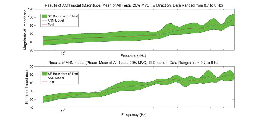
26 (b) Figure Performance Plots (a) DP Direction (b) IE Direction Therefore, all single-subject based models have reasonable performance in training the model. D. Tracking of Impedances in Frequency Domain: The impedance tracking in frequency domain shows the change of magnitude and phase of impedance with respect to frequency and the comparison between predictive outputs from models and original impedance collected from tests. The standard error boundaries of magnitude and phase of original impedance are also shown in the plots, they are used for deciding on reliability and accuracy of the method and models. The standard error are calculated using this equation: s SE, n s is the standard derivation of the sample and n is the number of the samples. Six plots were created for ANN model in both DP and IE directions to explain the tracking results of magnitude and phase of impedance in three muscle activation levels, separately. In each plot, 2 lines and a shaded area were drawn as follows: 1. The average magnitude or phase of original impedance from experiments (Red line): 5 rounds of the magnitude or phase of original impedance at a certain muscle activation level were averaged according to the frequency and shown as this red line. 2. The average magnitude or phase of predicted impedance from the model (Blue line): 5 25

27 rounds of the magnitude or phase of predicted impedance at a certain muscle activation level were averaged according to the frequency and shown as this blue line. 3. Standard error boundary of original impedance (Green shaded area): the upper limit of this area is the averaged magnitude or phase of original impedance from the tests at each frequency plus its standard error, and the lower limit of it is the averaged magnitude or phase of original impedance from the tests at each frequency minus its standard error. The x-axis of each plot is limited from 0.7 to 8 Hz. The impedance tracking in frequency domain is discussed in 3 aspects: standard error boundary, range of magnitude and phase, and break point. In DP direction of single-subject based model, almost all impedance tracking plots of both magnitude and phase have small standard error boundaries and the lines of predicted magnitude or phase from the model lie within those boundaries. It shows that the predicted impedance from the models track the results of experiments closely and the data collected in the tests are reliable enough to create the models. Only one subject (No.6 subject) has relative large standard error boundaries (more than 40% of the range of magnitude) in magnitude plots when the muscles are passive and 10% MVC (maximum voluntary contraction) compared to the other 9 subjects but those results are just 6% of all impedance plots, so they will not influence the reliability of data used in building the model. The ranges of phase and magnitude of impedance of 10 singlesubject based models in this direction are from 20 to 60 (magnitude) and 60 to 150 (phase), 35 to 175 and 40 to 85, 60 to 165 and 45 to 100 when muscles are passive, 10% MVC and 20% MVC, respectively. Comparing between these three muscle activation levels, the range of magnitude is higher as the muscle activation level is higher in most subjects except for only one subject (No.4 subject) has higher range in 10% MVC than 20% MVC; the passive muscle activation level typically has the largest range of phase, with smaller range in 20% MVC and the smallest range in 10%. 2 subjects have smallest (No.4 subject) or largest (No.9 subject) range of phase in 20% MVC. Moreover, most subjects didn t reach the break point, which means phase is 90. The number of subjects who reached the break point when muscles are passive, 10% MVC and 20% MVC are 7, 1 and 2. Therefore most subjects can t reach the break point when the muscles are active. The break points are located in 4-8 Hz, mostly in 5-6 Hz (6 subjects). For the IE direction, the magnitude and phase tracking plots have good tracking results as the model output lines almost coincide with the original test data lines and those model lines lie within the standard error boundaries. Most of the subjects also have small or acceptable (less than 1/3 of the range of magnitude or phase) standard error boundaries so the collected impedance in IE direction are suitable for building models as well. One subject (subject No.6) has relatively large (more than 1/3 of the range of magnitude or phase) standard error boundaries of magnitude in 10% MVC, 20% MVC and relatively large standard error boundaries of phase in 10% MVC. However, these exceptions are just 10% of all impedance tracking plots so the data from tests are still reliable in IE direction. The ranges of phase and magnitude of impedance in IE direction are 8 to 29 26

28 (magnitude) and 20 to 38 (phase), 9 to 44 and 16 to 35, 11 to 50 and 16 to 32 when muscles are passive, 10% MVC and 20% MVC, respectively. The change of ranges of magnitude in IE direction is the same as DP direction, the range of magnitude is higher as the muscle activation level is higher. However, different from the results in DP direction, there is no rule for majority of subjects for the change of ranges of phase in IE direction. Furthermore, no subject reach the break point (phase as 90) in any muscle activation level in IE direction. Comparing between DP and IE directions, the original impedance data in DP direction are better as the standard error boundaries of original impedance in IE direction are larger. The ranges of magnitude and phase in DP direction are also larger than the ranges in IE direction due to the larger magnitude and phase in DP direction. For the break point, although a few subjects reached it in certain muscle activation levels in DP direction, those situations are just very small part of all tracking plots, so the results in this aspect are close in both directions. The tracking plots (See Figure-6.4) of one representative single-subject based model (based on No.4 subejct) are shown below to clearly illustrate the results of impedance tracking in frequency domain. (a) 27

29 (b) (c) (d) 28

30 (e) (f) Figure Tracking of Impedances in Frequency Domain (a) Passive, DP Direction (b) 10% MVC, DP Direction (c) 20% MVC, DP Direction (d) IE Direction (e) 10% MVC, IE Direction (f) 20% MVC, IE Direction The standard error boundaries of magnitude and phase of the representative singlesubject based model are small in all muscle activation levels in both directions, the boundary is only a little bit larger but still acceptable when muscle is passive in IE direction (around 25% of range of phase). Its ranges of magnitude and phase in DP direction are 20 to 80 (magnitude) and 25 to 90 (phase), 50 to 225 and 20 to 70, 50 to 200 and 20 to 65 when the muscle activation level is passive, 10% MVC or 20% MVC; the ranges in IE direction are 10 to 38 and 33 to 58, 20 to 51 and 17 to 45, 21 to 51 and 17 to 40 for the three muscle activation levels, respectively. This model only reached break point at about 8Hz when muscles are passive in DP direction, all the other muscle situations didn t reach the break point. Therefore, the impedance data from experiments of this model are good enough to build the model while the data built the single-subject 29

31 based model have smaller standard error boundaries, and this model only reached break point at about 8Hz when muscles are passive in DP direction. All the results above proves that the original impedance from experiments are reliable in building the ANN models and those created models can precisely track the original impedance. VII. Conclusion and Future Works: This paper has developed models to describe the nonlinear relationship between the mechanical impedance of the human ankle within a range of frequency and the RMS (root mean square) value of the Electromyography (EMG) signals of the muscles of human ankle using Artificial Neural Network (ANN). The models produced the characterization of mechanical impedance in two degrees of freedom simultaneously dorsiflexion-plantarflexion (DP) and inversion-eversion (IE) at 3 different muscle activation levels. The regression R values of all four datasets of almost all single-subject based models in both directions are more than 0.9. The actual fitting lines and ideal fitting lines of four datasets of the representative single-subject based model almost coincide with each other, the original data points from the test also evenly located in the full data range. It indicates a very close relationship between outputs from the models and target impedance and the outputs from the ANN model accurately tracks the target impedance from the experiments. The regression R values are close in DP and IE directions, this may illustrates that the R values are not influenced by the direction and it is good enough in both directions. More than half of the outputs from all single-subject based models are very accurate in both directions comparing to the original test data with relative errors less than 10% and those numbers are over 65% for most model or even over 85%. For the outputs with relative errors less than 15%, the proportion increases to around or over 80% in most models in both directions and part of models have approximately 90%-95% qualified outputs. Moreover, almost all models have more than 90% outputs with relative errors less than 30% in both directions. The errors of the models were not influenced by the directions, and the relative errors of most models are larger if the proportions are smaller, which means accurate outputs have larger proportion. The error histograms also give exactly the same results. Therefore all the ANN models have sufficient accuracy in predicting the results in both DP and IE directions as they have small enough relative errors. The MSEs of all data of all models are relatively small compared to the magnitude of target impedance. They are also smaller in IE direction than DP as the magnitudes of impedance in DP direction are typically larger than the ones in IE direction. The iterations 30

32 to complete training the model are not influenced by the direction, and it doesn t determine the final MSEs and regression R values as well. Moreover, the characteristics of test dataset errors and the validation dataset errors are similar to each other for all models, and no significant overfitting has occurred when the training reached the best validation performance. It proves that all single-subject based models have reasonable performance in training the model. In both DP and IE direction of most models, almost all impedance tracking plots of both magnitude and phase have small standard error boundaries, the lines of predicted magnitude or phase from the model almost coincide with the original test data lines and lie within those boundaries. It shows that the predicted impedance from the models track the results of experiments closely and the data collected in the tests are reliable enough to create the models. Comparing between these three muscle activation levels, the range of magnitude is higher as the muscle activation level is higher in most subjects. The ranges of magnitude and phase in DP direction are also larger than the ranges in IE direction due to the larger magnitude and phase in DP direction. Moreover, most subjects didn t reach the break point, which means phase is 90. All the results of analysis of the model proved that the developed models have enough accuracy and feasibility to characterize the mechanical impedance of the human ankle with respect to EMG. In the future works, more subjects with more diversity of backgrounds may be included to create more complex ANN models. During these processes, more degrees of freedom of ankle movement, more muscle activation levels, more observed muscles will be considered into building ANN model as well. As all the models researched before were focused the data collected when the subjects were sitting still, the ANN model based on the data from the subjects in walking status will be built and analyzed in the next step. We envision that the combination of research of mechanical impedance of the human ankle and neural networks will greatly facilitate the development of the areas of assistive robotics, human healthy and human recovery from injuries. 31

33 Acknowledgements I would like to acknowledge the support of my advisor Dr. Mo Rastgaar, and my thesis committee members Dr. Nina Mahmoudian, and Dr. Tomas B. Co. Also, I would like to thank Evandro Ficanha for his invaluable help with the different experiments on the human subjects. This research was supported by Human-Interactive Robotics Lab (HIRo Lab) at the Department of Mechanical Engineering-Engineering Mechanics, Michigan Technological University, and is partially supported by the National Science Foundation under CAREER Grant No

34 References [1] A. Lamontagne, F. Malouin, and C. L. Richards, "Viscoelastic behavior of plantar flexor muscle-tendon unit at rest," The Journal of Orthopaedic and Sports Physical Therapy, vol. 26, pp , [2] J. Harlaar, J. Becher, C. Snijders, and G. Lankhorst, "Passive stiffness characteristics of ankle plantar flexors in hemiplegia," Clinical Biomechanics, vol. 15, pp , [3] B. Singer, J. Dunne, K. Singer, and G. Allison, "Evaluation of triceps surae muscle length and resistance to passive lengthening in patients with acquired brain injury," Clinical Biomechanics vol. 17, pp , [4] S. G. Chung, E. Rey, Z. Bai, E. J. Roth, and L.-Q. Zhang, "Biomechanic changes in passive properties of hemiplegic ankles with spastic hypertonia," Archives of Physical Medicine and Rehabilitation, vol. 85, pp , [5] S. J. Rydahl and B. J. Brouwer, "Ankle stiffness and tissue compliance in stroke survivors: A validation of myotonometer measurements," Archives of Physical Medicine and Rehabilitation, vol. 85, pp , [6] T. Kobayashi, A. K. L. Leung, Y. Akazawa, M. Tanaka, and S. W. Hutchins, "Quantitative measurements of spastic ankle joint stiffness using a manual device: A preliminary study," Journal of Biomechanics, vol. 43, pp , [7] I. W. Hunter and R. E. Kearney, "Dynamics of Human Ankle Stiffness: Variation with Mean Ankle Torque," Journal of Biomechanics, vol. 15, pp , [8] R. E. Kearney and I. W. Hunter, "Dynamics of human ankle stiffness: Variation with displacement amplitude," Journal of Biomechanics, vol. 15, pp , [9] P. L. Weiss, R. E. Kearney, and I. W. Hunter, "Position dependence of ankle joint dynamics I. Passive mechanics," Journal of Biomechanics, vol. 19, pp , [10] P. L. Weiss, R. E. Kearney, and I. W. Hunter, "Position dependence of ankle joint dynamics II. Active mechanics," Journal of Biomechanics, vol. 19, pp , [11] M. M. Mirbagheri, R. E. Kearney, and H. Barbeau, "Quantitative, objective measurement of ankle dynamic stiffness: intra-subject reliability and intersubject variability," in 18th Annual International Conference of the IEEE Engineering in Medicine and Biology Society, Amsterdam, [12] R. E. Kearney, R. B. Stein, and L. Parameswaran, "Identification of intrinsic and reflex contributions to human ankle stiffness dynamics," IEEE transactions on biomedical engineering, vol. 44, pp , [13] T. Sinkjaer, E. Toft, S. Andreassen, and B. C. Hornemann, "Muscle stiffness in human ankle dorsiflexors: Intrinsic and reflex components," Journal of Neurophysiology, vol. 60, pp , [14] R. F. Kirsch and R. E. Kearney, "Identification of time-varying stiffness dynamics of the human ankle joint during an imposed movement," Experimental Brain Research, vol. 114, pp , [15] D. A. Winter, A. E. Patla, S. Rietdyk, and M. G. Ishac, "Ankle muscle stiffness in 33

35 the control of balance during quiet standing," Journal of Neurophysiology, vol. 85, pp [16] P. G. Morasso and V. Sanguineti, "Ankle muscle stiffness alone cannot stabilize balance during quiet standing," Journal of Neurophysiology, vol. 88, [17] I. D. Loram and M. Lakie, "Human balancing of an inverted pendulum: position control by small, ballistic-like, throw and catch movements," The Journal of Physiology, vol. 540, pp , [18] I. D. Loram and M. Lakie, "Direct measurement of human ankle stiffness during quiet standing: the intrinsic mechanical stiffness is insufficient for stability," The Journal of Physiology, vol. 545, pp , [19] R. Davis and P. DeLuca, "Gait characterization via dynamic joint stiffness," Gait and Posture, vol. 4, pp , [20] M. Palmer, "Sagittal plane characterization of normal human ankle function across a range of walking gait speeds," MS, Mechanical Engineering, Massachusetts Institute of Technology, Cambridge, MA, [21] A. H. Hansena, D. S. Childress, S. C. Miff, S. A. Gard, and K. P. Mesplay, "The human ankle during walking: implication for design of biomimetic ankle prosthesis," Journal of Biomechanics, vol. 37, pp , [22] C. T. Farley, R. Blickhan, J. Saito, and C. R. Taylor, "Hopping frequency in humans: a test of how springs set stride frequency in bouncing gaits," Journal of Applied Physiology, vol. 71, pp , [23] C. T. Farley and O. González, "Leg stiffness and stride frequency in human running," Journal of Biomechanics, vol. 29, pp , [24] A. Saripalli and S. Wilson, "Dynamic Ankle Stability and Ankle Orientation," presented at the 7th Symp. Footwear Biomech. Conf., Cleveland, OH, [25] S. M. Zinder, K. P. Granata, D. A. Padua, and B. M. Gansneder, "Validity and reliability of a new in vivo ankle stiffness measurement device," Journal of Biomechanics, vol. 40, pp , [26] A. Roy, H. I. Krebs, D. J. Williams, C. T. Bever, L. W. Forrester, R. M. Macko, et al., "Robot-aided neurorehabilitation: A novel robot for ankle rehabilitation," IEEE Transactions on Robotics and Automation, vol. 25, pp , [27] A. Arndt, P. Wolf, A. Liu, C. Nester, A. Stacoff, R. Jones, et al., "Intrinsic foot kinematics measured in vivo during the stance phase of slow running," Journal of Biomechanics, vol. 40, pp , [28] P. Ho, H. Lee, H. I. Krebs, and N. Hogan, "Directional Variation of Active and Passive Ankle Static Impedance," in ASME Dynamic Systems and Control Conference, Hollywood, CA, [29] P. Ho, H. Lee, M. Rastgaar, H. I. Krebs, and N. Hogan, "The Interpretation of the Directional Properties of Voluntarily Modulated Human Ankle Impedance," in ASME Dynamic Systems and Control Conference, Cambridge, MA, [30] H. Lee, P. Ho, H. I. Krebs, and N. Hogan, "The multi-variable torquedisplacement relation at the ankle," in ASME Dynamic Systems and Control Conference, Hollywood, CA, [31] H. Lee, P. Ho, M. Rastgaar, H. I. Krebs, and N. Hogan, "Quantitative Characterization of Steady-State Ankle Impedance with Muscle Activation," in ASME Dynamic Systems and Control Conference Cambridge, MA,

36 [32] H. Lee, P. Ho, M. Rastgaar, H. I. Krebs, and N. Hogan, "Multivariable static ankle mechanical impedance with relaxed muscles," Journal of Biomechanics, vol. 44, pp , [33] H. Lee, P. Ho, M. Rastgaar, H. I. Krebs, and N. Hogan, "Multivariable static ankle mechanical impedance with active muscles," IEEE Transaction on Neural Systems and Rehabilitation Engineering, vol. 22, pp , [34] H. Lee and N. Hogan, "Modeling Dynamic Ankle Mechanical Impedance in Relaxed Muscle," in ASME Dynamic Systems and Control Conference, Arlington, VA, [35] H. Lee and N. Hogan, "Investigation of Human Ankle Mechanical Impedance During Locomotion Using a Wearable Ankle Robot," in 2013 IEEE International Conference on Robotics and Automation (ICRA), Karlsruhe, Germany, [36] H. Lee, H. I. Krebs, and N. Hogan, "A Novel Characterization Method to Study Multivariable Joint Mechanical Impedance," in The Fourth IEEE RAS/EMBS International Conference on Biomedical Robotics and Biomechatronics, Roma, Italy, [37] H. Lee, H. I. Krebs, and N. Hogan, "Multivariable Dynamic Ankle Mechanical Impedance with Relaxed Muscles," IEEE Transactions on Neural Systems and Rehabilitation Engineering, [38] H. Lee, H. I. Krebs, and N. Hogan, "Multivariable Dynamic Ankle Mechanical Impedance with Active Muscles," IEEE Transactions on Neural Systems and Rehabilitation Engineering, vol. 22, pp , [39] H. Lee, T. Patterson, J. Ahn, D. Klenk, A. Lo, H. I. Krebs, et al., "Static Ankle Impedance in Stroke and Multiple Sclerosis: A Feasibility Study," presented at the Annual International Conference of the IEEE EMBS, Boston, Massachusetts, [40] M. Rastgaar, P. Ho, H. Lee, H. I. Krebs, and N. Hogan, "Stochastic estimation of multi-variable human ankle mechanical impedance," in ASME Dynamic Systems and Control Conference, Hollywood, CA, [41] M. Rastgaar, P. Ho, H. Lee, H. I. Krebs, and N. Hogan, "Stochastic estimation of the multi-variable mechanical impedance of the human ankle with active muscles," in ASME Dynamic Systems and Control Conference, Boston, MA, [42] A. Roy, H. I. Krebs, C. T. Bever, L. W. Forrester, R. F. Macko, and N. Hogan, "Measurement of passive ankle stiffness in subjects with chronic hemiparesis using a novel ankle robot," J Neurophysiol, vol. 105, pp , [43] E. M. Ficanha and M. R. Aagaah, "Stochastic Estimation of Human Ankle Mechanical Impedance in Medial-lateral Direction," presented at the ASME Dynamic Systems and Control Conference (DSCC), San Antonio, TX, [44] M. Rastgaar, H. Lee, E. M. Ficanha, P. Ho, H. I. Krebs, and N. Hogan, "Multi- Directional Dynamic Mechanical Impedance of the Human Ankle; a Key to Anthropomorphism in Lower Extremity Assistive Robots," in Neuro-Robotics: From Brain Machine Interfaces to Rehabilitation Robotics, P. Artemiadis, Ed., ed New York: Springer, 2014, pp [45] H. Lee and N. Hogan, "Time-Varying Ankle Mechanical Impedance during Human Locomotion," IEEE Transactions on Neural Systems and Rehabilitation Engineering,

37 [46] H. Lee, H. I. Krebs, and N. Hogan, "Linear Time-Varying Identification of Ankle Mechanical Impedance During Human Walking," in ASME th Annual Dynamic Systems and Control Conference, Fort Lauderdale, FL, USA, [47] E. Rouse, L. Hargrove, E. Perreault, and T. Kuiken, "Estimation of Human Ankle Impedance During Walking Using the Perturberator Robot," presented at the Fourth IEEE RAS/EMBS International Conference on Biomedical Robotics and Biomechatronics, Roma, Italy, [48] E. Rouse, L. Hargrove, E. Perreault, M. Peshkin, and T. Kuiken, "Development of a Mechatronic Platform and Validation of Methods for Estimating Ankle Stiffness during the Stance Phase of Walking," Journal of biomechanical engineering, vol. 135, pp , [49] E. Ficanha, M. Rastgaar, and K. R. Kaufman, "Gait Emulator for Evaluation of Ankle-Foot Prostheses Capable of Turning," presented at the Design of Medical Device Conference, accepted, Minneapolis, MN, [50] Jiuchao Feng, Chi K. Tse, Francis C. M. Lau, "A Neural-Network-Based Channel- Equalization Strategy for Chaos-Based Communication Systems", IEEE transactions on circuits and systems. I, Fundamental theory and applications (Volume 50, No.7): , [51] De Jesús, O., J.M. Horn, M.T. Hagan, "Analysis of Recurrent Network Training and Suggestions for Improvements", Neural Networks, Proceedings. IJCNN '01. International Joint Conference (Volume 4): , [52] Horn, J.M., O. De Jesús and M.T. Hagan, "Spurious Valleys in the Error Surface of Recurrent Networks - Analysis and Avoidance", Neural Networks, IEEE Transactions (Volume 20, Issue 4): , [53] Gianluca Pollastri, "Improving the prediction of protein secondary structure in three and eight classes using recurrent neural networks and profiles", Proteins: Structure, Function, and Bioinformatics (Volume 47, Issue 2): , [54] Yasuharu Koike, Mitsuo Kawato, "Estimation of Movement from Surface EMG Signals Using a Neural Network Model", Biomechanics and Neural Control of Posture and Movement: , [55] Guozheng Xu, Aiguo Song, Huijun Li, "Adaptive Impedance Control for Upper- Limb Rehabilitation Robot Using Evolutionary Dynamic Recurrent Fuzzy Neural Network", Journal of Intelligent & Robotic Systems (Volume 62, Issue 3-4): , [56] Seul Jung, Sun Bin Yim and Hsia, T.C., "Experimental studies of neural network impedance force control for robot manipulators", Robotics and Automation, Proceedings 2001 ICRA. IEEE International Conference (Volume 4): , [57] Seul Jung and Hsia, T.C., "Neural network impedance force control of robot manipulator", Industrial Electronics, IEEE Transactions (Volume 45, Issue 3): , [58] Kuen-Chang Hsieh, "The novel application of artificial neural network on bioelectrical impedance analysis to assess the body composition in elderly", Nutrition Journal 2013 (Volume 12),

38 Appendix A: Collected Data of All Ten Subjects A. Regression values, R: Table A.1 - Regression Values of All Models Subject No. Subject 1 Subject 2 Subject 3 Subject 4 Subject 5 Subject 6 Subject 7 Subject 8 Subject 9 Subject 10 Training Data DP Direction Validation Data Test Data All Data Training Data IE Direction Validation Data Test Data All Data

39 B. Distribution of Errors: a. DP Direction: Table A.2 - Relative Errors of All Models (a) Number of Samples, DP Direction (b) Proportion of Samples, DP Direction (c) Number of Samples, IE Direction (d) Proportion of Samples, IE Direction Number of Samples Subject No. less more less less 11% to 16% to 21% to than than than than 15% 20% 30% 10% 30% 15% 30% Subject Subject Subject Subject Subject Subject Subject Subject Subject Subject (a) Proportion of All Samples Subject No. less more less less 11% to 16% to 21% to than than than than 15% 20% 30% 10% 30% 15% 30% Subject % 7.37% 14.39% 7.81% 9.91% 74.91% 90.09% Subject % 13.07% 6.32% 7.37% 8.51% 77.81% 91.49% Subject % 9.30% 3.77% 2.19% 0.61% 93.42% 99.39% Subject % 11.23% 3.25% 2.19% 0.61% 93.95% 99.39% Subject % 11.93% 5.79% 6.75% 6.84% 80.61% 93.16% Subject % 12.37% 8.95% 7.28% 5.88% 77.89% 94.12% Subject % 11.58% 5.00% 4.65% 3.16% 87.19% 96.84% Subject % 14.91% 9.04% 9.39% 7.54% 74.04% 92.46% Subject % 9.30% 4.74% 3.95% 1.49% 89.82% 98.51% Subject % 10.70% 6.14% 3.95% 1.84% 88.07% 98.16% (b) 38

40 b. IE Direction: Number of Samples Subject less more less less No. 11% to 16% to 21% to than than than than 15% 20% 30% 10% 30% 15% 30% Subject Subject Subject Subject Subject Subject Subject Subject Subject Subject (c) Proportion of All Samples Subject less more less less No. 11% to 16% to 21% to than than than than 15% 20% 30% 10% 30% 15% 30% Subject % 13.42% 10.53% 9.12% 14.21% 66.14% 85.79% Subject % 15.26% 7.72% 6.67% 4.12% 81.49% 95.88% Subject % 10.88% 4.91% 2.81% 1.84% 90.44% 98.16% Subject % 8.25% 2.19% 1.84% 0.61% 95.35% 99.39% Subject % 13.95% 7.72% 8.07% 6.67% 77.54% 93.33% Subject % 13.68% 7.11% 8.51% 6.14% 78.25% 93.86% Subject % 14.82% 7.81% 9.47% 10.79% 71.93% 89.21% Subject % 16.32% 10.18% 8.68% 7.72% 73.42% 92.28% Subject % 9.21% 4.65% 4.56% 2.63% 88.16% 97.37% Subject % 10.26% 6.05% 3.77% 3.68% 86.49% 96.32% (d) 39

41 C. Mean Squared Errors: Table A.3 - MSEs of All Models Subejct No. Subject 1 Subject 2 Subject 3 Subject 4 Subject 5 Subject 6 Subject 7 Subject 8 Subject 9 Subject 10 Training Data DP Direction Validation Data Test Data Training Data IE Direction Validation Data Test Data

42 D. Performance: Table A.4 - Performance of All Models Subject No. Subject 1 Subject 2 Subject 3 Subject 4 Subject 5 Subject 6 Subject 7 Subject 8 Subject 9 Subject 10 Best Validation Performance (Smallest MSE) DP Direction Iterations for Completing Training Iterations to Reach Smallest MSE Best Validation Performance (Smallest MSE) IE Direction Iterations for Completing Training Iterations to Reach Smallest MSE

43 Appendix B: Figures of All Single-Subject Based Models that Not Shown in the Paper A. Regression Plots: (a) 42

44 (b) (c) 43

45 (d) (e) 44

46 (f) (g) 45

47 (h) (i) 46

48 (j) (k) 47

49 (l) (m) 48

50 (n) (o) 49

51 (p) (q) 50

52 (r) Figure B.1 Regression Plots (a) No.1 subject, DP direction (b) No.1 subject, IE direction (c) No.2 subject, DP direction (d) No.2 subject, IE direction (e) No.4 subject, DP direction (f) No.4 subject, IE direction (g) No.5 subject, DP direction (h) No.5 subject, IE direction (i) No.6 subject, DP direction (j) No.6 subject, IE direction (k) No.7 subject, DP direction (l) No.7 subject, IE direction (m) No.8 subject, DP direction (n) No.8 subject, IE direction (o) No.9 subject, DP direction (p) No.9 subject, IE direction (q) No.10 subject, DP direction (r) No.10 subject, IE direction 51

53 B. Error Histogram: (a) (b) (c) 52

54 (d) (e) (f) 53

55 (g) (h) (i) 54

56 (j) (k) (l) 55

57 (m) (n) (o) 56

58 (p) (q) (r) 57

59 Figure B.2 Error Histogram (a) No.1 subject, DP direction (b) No.1 subject, IE direction (c) No.2 subject, DP direction (d) No.2 subject, IE direction (e) No.3 subject, DP direction (f) No.3 subject, IE direction (g) No.5 subject, DP direction (h) No.5 subject, IE direction (i) No.6 subject, DP direction (j) No.6 subject, IE direction (k) No.7 subject, DP direction (l) No.7 subject, IE direction (m) No.8 subject, DP direction (n) No.8 subject, IE direction (o) No.9 subject, DP direction (p) No.9 subject, IE direction (q) No.10 subject, DP direction (r) No.10 subject, IE direction C. Performance Plots: (a) (b) 58

60 (c) (d) (e) 59

61 (f) (g) (h) 60

62 (i) (j) (k) 61

63 (l) (m) (n) 62

64 (o) (p) (q) 63

65 (r) Figure B.3 Performance Plots (a) No.1 subject, DP direction (b) No.1 subject, IE direction (c) No.2 subject, DP direction (d) No.2 subject, IE direction (e) No.4 subject, DP direction (f) No.4 subject, IE direction (g) No.5 subject, DP direction (h) No.5 subject, IE direction (i) No.6 subject, DP direction (j) No.6 subject, IE direction (k) No.7 subject, DP direction (l) No.7 subject, IE direction (m) No.8 subject, DP direction (n) No.8 subject, IE direction (o) No.9 subject, DP direction (p) No.9 subject, IE direction (q) No.10 subject, DP direction (r) No.10 subject, IE direction D. Tracking of Impedances in Frequency Domain: (a1) 64

66 (a2) (a3) 65

67 (a4) (a5) (a6) 66

68 (b1) (b2) (b3) 67

69 (b4) (b5) (b6) 68

70 (c1) (c2) (c3) 69

71 (c4) (c5) (c6) 70

72 (d1) (d2) (d3) 71

73 (d4) (d5) (d6) 72

74 (e1) (e2) (e3) 73

75 (e4) (e5) (e6) 74