12. Thermal and scalar field analysis

Transcription

1 2. THERMAL AND SCALAR FIELD ANALYSIS INTRODUCTION GENERAL FIELD PROBLEM COMMON FLUX COMPONENTS GALERKIN INTEGRAL FORM GALERKIN INTEGRAL FORM* ORTHOTROPIC TWO-DIMENSIONAL FIELDS CORRESPONDING ELEMENT AND BOUNDARY MATRICES NUMERICAL EVALUATION OF THE JACOBIAN MATRIX JACOBIAN MATRIX FOR EQUAL SPACE DIMENSIONS PHYSICAL SPACE > PARAMETRIC SPACE: FIELD FLUX VECTOR AT A POINT EVALUATION OF INTEGRALS WITH CONSTANT JACOBIAN SYMMETRY AND ANTI-SYMMETRY VISCOUS FLUID FLOW IN A CHANNEL... ERROR! BOOKMARK NOT DEFINED. 2.5 AXISYMMETRIC FIELDS SUMMARY Thermal and scalar field analysis 2. Introduction: Field analysis covers many areas of physics and engineering governed by the partial differential equations known as the Helmholtz Equation, the Poisson Equation, and the Laplace Equation. These equations define several physical problems with scalar unknowns. They describe heat transfer by conduction, convection and radiation; the torsion of non-circular shafts, ideal fluid motion by a velocity potent or by a stream function; seepage of a viscous fluid through a porous media; electrostatics; magnetostatics; and others. As their names imply, these equations have been in use for more than two-hundred years and a huge number of solutions have been published using analytical and numerical approaches. The application of these problems requires the satisfaction of the essential boundary conditions and/or nonessential boundary conditions described earlier. Many of the early analytic models dealt with domains that were assumed to contained a single, constant, isotropic material property, say κ, that defined a scalar unknown, say u, driven by a source term, say Q, and satisfying the two-dimensional homogeneous Poisson equation: 2 u u Q(x, y) = 2 κ

2 In applications where the material property was non-homogeneous or varied with position the governing equation changed to a more difficult form: κ(x, y) ( 2 u u 2) = Q(x, y) When the application involved materials with two orthotropic properties, like a layered soil or wood, the governing equation again takes on a more complicated form κ x (x, y) 2 u 2 + κ y(x, y) 2 u = Q(x, y) 2 The most general form of the scalar field equations involve fully directionally dependent (anisotropic) and position dependent (non-homogeneous) material properties associated with the highest derivatives in the governing differential equation. Relatively few materials are isotropic and homogeneous. Modern materials science creates new advanced materials and almost all of those materials are anisotropic. Any anisotropic material has an orthogonal set of principal directions. The material properties are experimentally measured with respect to those axes. Next, the fully anisotropic material formulation of the scalar field problem is presented and converted to an equivalent finite element formulation. The boundary conditions for second order field problems are the same as discussed for the one-dimensional equations, except that some involve the derivative of the solution in the direction normal to the boundary where they are applied. They are sketched in Fig The default boundary condition on any surface is that the normal gradient of the solution (and the normal flux) are zero. This is called the natural boundary condition (NatBC), and it does not require any input data. It is usually necessary to have essential boundary conditions (EBC) that specify the value of the solution at one or more points. Often the normal flux entering the body is known and is specified as one of the nonessential boundary conditions (NBC). It indirectly specifies the normal gradient of the solution at a point. The more complicated nonessential condition is the mixed condition that couples the normal gradient of the solution to the unknown value of the solution. That mixed boundary condition (MBC) usually occurs as a convection boundary condition (CBC) or as a radiation boundary condition (RBC) in nonlinear applications. Only the presence of a radiation condition requires the use of the Kelvin temperature scale. Figure 2. Natural, essential, known flux, and convection boundary conditions 2.2 General field problem: The anisotropic (directionally dependent) Helmholtz equation is a good example of one of the most common problems in engineering and physics that solves for scalar unknowns. The one-dimensional form was covered earlier. In three-dimensions the transient model equation is 2

3 ([κ] T u(x, y, z, τ)) + m v T u(x, y, z, τ) a u(x, y, z, τ) Q(x, y, z, τ) = ρ τ (2.2-) where τ denotes time. The square matrix [κ] usually contains the symmetric, directionally dependent material properties, like shown in Fig. 2.2-, evaluated in the system coordinate directions: k xx k xy k xz [κ] = [ k xy k yy k yz ] = [κ] T, κ > (2.2-2) k xz k yz k zz Onsager s reciprocal relation requires the symmetry of the material matrix (and tensor). However, for some physical problems, like geophysical flows, it is quite difficult to reduce the necessary experimental measurements into a symmetric form. Not forcing the data into a symmetric form is a poor practice. It may yield computable answers, if κ >, but using a nonsymmetric also renders the system square matrix non-symmetric and significantly increases the solution computational time, and violates fundamental principles of thermodynamics. In some fields of study authors pre-multiply by (or factor outside) an isotropic material property, like a fluid viscosity, when defining [κ]. For an isotropic material the property matrix is simply [κ] k[i], the single property times the identity matrix. For an orthotropic material, with the principle directions parallel to the system axes, the material array is diagonal k xx [κ] = [ k yy ], κ > k zz Figure 2.2- (and 5.7-) Element principle material directions The x-, y-,z-directions are the ones used to define the shape of the solution domain, and its boundary. If the domain contains a material with directionally dependent (anisotropic) properties then the material principle directions and the measured properties, say [κ PD ], must be transformed into the system coordinate system using the direction cosines between the two coordinate systems. The first term in (2.2-) is a scalar inner product of the material property array pre- and post-multiplied by the gradient vector. As a scalar that product is the same in any coordinate system. Thus, it can be shown that system properties are obtained from the principle 3

4 direction properties by a coordinate transformation (for any vector): PD = T PD. The scalar product is [κ] T = T [κ] T = T PD [κ PD ] PD = T (T T PD [κ PD ] T PD ) For a two-dimensional problem, the vector transformation matrix is [κ] = T T PD [κ PD ] T PD (2.2-3) cos θ sin θ T PD = [ sin θ cos θ ] = [cos θ xx cos θ xy ], (2.2-) cos θ yx cos θ yy where θ xy (x, y) is the angle from the system x-axis to the principle direction y-axis. For some materials, like plywood, the angle is the same throughout the part but it is not rare for the angle to vary continuously, as in filament wound composites. Then the property is viewed as a variable coefficient in the PDE. For a three-dimensional solid the transformation matrix, at any point, is a 3 3 matrix containing the direction cosines from the system axes to the principle direction axes. For each element with constant anisotropic properties the six material coefficients and the direction angles from the system axes would be required as input data. Some geologic rock structures and filament wound solids have a continuously changing orientation of the principle directions. They would also have to be input at every quadrature point or averaged to a single element direction value. That represents a large amount of data, by gives the finite element method the ability to give accurate solutions to extremely complicated real-world problems. The gradient operator in (2.2-) is T = { } = (2.2-5) z and, a is a convection like term, Q is a source rate per unit volume, ρ is a mass density term, and τ denotes time. Often there is a known velocity vector, v, with an associated transport property, m. If they are not zero, then this is known as an advection-diffusion equation otherwise it is just called the diffusion equation. If the velocity is not zero or quite small relatively, then the standard Galerkin MWR covered here will lead to widely oscillating solutions and special Petrov-Galerkin method must be used instead to bias the interpolations in the direction of the incoming velocity. If a = and m =, it is often called the Poisson equation. If just m =, (2.2-) is known as the Helmholtz Equation. If the Helmholtz Equation contains the coefficient a as an unknown system constant (eigenvalue) to be determined then it requires an eigen-problem analysis which utilizes the same finite element matrices covered here. The solution of eigen-problems is addressed in Chapter 2. For orthotropic materials [κ] is a diagonal array. For isotropic materials it becomes a single value times an identity matrix. In two-dimensions the second order operator becomes [κ] T u = (k xx ) + (k xy ) + (k yx ) + (k yy ) (2.2-6) In the prior one-dimensional formulations only the first term was included.

5 Example 2.2- Given: Field measurements from a geologic structure are passed through different software to fit the permeability matrices. The two results are κ A and κ B listed below. Which is best suited for a porous media flow study? κ A = [ ], κ B = [ ] Solution: Both matrices have a positive determinant of about 3, but κ B does not satisfy the Onsager symmetry requirement, Therefore, κ A are the preferred data. 2.3 Common flux components: In this chapter the unknown, u(x, y, z), is a scalar which may or may not have physical meaning. The components of the solution gradient, combined with any physical properties, usually do have physical meaning as components of a vector or tensor quantity, as sketched in Fig Here some of the more common two-dimensional relations are summarized. Figure 2.3- Solution gradient defines physical flux components In heat transfer Fourier s Law defines a heat flux vector per unit area, q, in terms of the gradient as q = { q x q } = q = [κ] T u = [ k xx k xy ] { } (2.3-) y k yy where [κ] contains the anisotropic thermal conductivity coefficients, u represents the temperature, and where the area is normal to the gradient vector. Often, the heat flow crossing a surface has importance. The heat flow crossing a surface is the integral, over the surface, of the normal component of the heat flux vector: k xy f = q n ds = q S S n ds (2.3-2) For fluid flow through a porous media Darcy s Law has the same form as (2.3-), but with q being the fluid velocity vector at the point where the gradient is computed. The material media properties in [κ] are the anisotropic permeability coefficients, and u represents the pressure at the point. The flow, f, is the volume of fluid that crosses the surface. 5

6 For the analysis of the concentration of substances Fick s First Law has the same form as (2.3-), with q being the diffusion flux vector which measures the amount of a substance, per unit area, that will flow through during a unit time interval. The solution, u, is the concentration (the amount of the substance per unit volume). The [κ] array contains the diffusivity (diffusion coefficients) at the point. For electrostatics, u corresponds to the voltage, [κ] contains the anisotropic electric conductivities, and q gives the electric charge flux vector. In some applications u represents a non-physical mathematical potential and [κ] contains zeros and ones that convert the gradient of the potential into physical components. In the study of the torsion of a straight non-circular shaft (along the z-axis), u represents a stress function which is zero on the outer boundary of the cross-section and its gradient components are re-arranged by [κ] to define the shear stress components in the plane of the cross-section: τ = { τ zx τ } = [ zy ] { } (2.3-3) The applied torque acting along the shaft is twice the integral of the stress function T = 2 u(x, y)da A (2.3-) Similarly, in potential (inviscid fluid) flow u corresponds to a non-physical velocity potential whose gradient components are the components of the velocity vector ([κ] = [I]). Then q n is the velocity component normal to a surface and corresponds to the volume of flow entering the domain. 2. Galerkin integral form: Applying the Galerkin MWR only the first term has additional components that will define additional terms in the element matrices. That integral is Applying Green s Theorem this becomes I k = u ( Γ I k u( [κ] T u) d (2.-) [κ] T u) n dγ u( [κ] T u) d (2.-2) where Γ is the boundary of the domain, and the unit normal vector on the boundary is n. The boundary term introduces the derivatives normal to the boundary and the material property at the surface in the direction of its normal vector: [κ] T u n = (k xx + k yx ) n x + (k yy + k xy ) n y k n n (2.-3) The scalar material property at a point in the direction of any unit vector n is k n = n T [κ]n. That product appears in the nonessential boundary conditions (including any mixed boundary conditions). Once again, when an essential boundary condition (on u on Γ u ) is specified and the normal flux (k n n on Γ NBC ) will be recovered as a reaction. 6

7 u ( Γ [κ] T u) n dγ = u ( Γ k n ) dγ (2.-) n The most common nonessential boundary condition is that of heat convection on the surface of a heat conducting solid. Then the mixed non-essential boundary condition is of the form k n n = hb (u u b ) (2.-5) and requires boundary segment matrices that integrate the data, h b and/or u b, over the boundary segment. For a three-dimensional analysis the boundary segment is most likely the face of some element. In a two-dimensional analysis the boundary segment is most likely one or more of the edges of the element. But if the 2-D element were part of a cooling fin the boundary segment could include the front and or back surface of the element. These are mainly modeling details, but the programmer must allow for any valid description of a boundary segment. When the finite element method is applied (below) to this three-dimensional equation the same element matrices occur as with the one-dimensional models. In one-dimension the nonessential boundary conditions occurred at a point (actually the integral over an area at the point), but in higher dimensional applications they enter as integrals over curves or surfaces. Conceptually, the second derivative term in the original equation leads to the same symbolic element square matrix as in the one-dimensional case. The differences are that the arrays are larger in size and the integration takes place over an area or volume: u( [κ] T u) d S e = κ e B e d (2.-6) e Here, the symbol B e arises from a differential operator, in this application it is the gradient, acting on the interpolated solution. Inside each element B e T T u = T H e (x, y, z) u e B e (x, y, z) u e H e (x, y, z) B e [ H e (x, y, z) ] (2.-6) H e (x, y, z) z Before, the material data involved a scalar, but now they become a square symmetric matrix, κ e. To be a valid matrix product in (2.-6) the number of rows in the operator matrix, B e, must be the same as those in κ e. Here, it will be shown below that number is the same as the physical space dimension, n s. However, in later applications the number of rows in B e is larger, say n r n s. The enlarged size of the arrays combined with any curved element geometry means that the above element integral is almost always evaluated numerically in practice. The exceptions are the three-node triangle and the four-node tetrahedron that have constant Jacobians. Those two elements were used in the first published solutions of two- and three-dimensional finite element solutions of field problems and eigen-problems. 2.5 Galerkin integral form*: From (2.-) the initial Galerkin method gives the integral I = u[ ([κ] T u) + m v T u a u Q ρ τ] d = (2.5-) 7

8 As usual, the first term containing the highest derivatives is integrated by parts via Green s theorem. First, it will be re-arranged using the following identity: [u([κ] T u)] = u ([κ] T u) + u ([κ] T u) I κ = u[ ([κ] T u)] d = [u([κ] T u)] d u ([κ] T u) d For any vector, V d = VT d = Γ n V T d = n V dγ and the first volume integral Γ is transformed into a boundary integral containing the nonessential boundary conditions I κ = [n T u([κ] T u)] dγ Γ u ([κ] T u) d I κ = u(k nn n) dγ u ([κ] T u) d Γ (2.5-2) which means that on the boundary either the value of the solution, u, is specified or the normal flux per unit area is given: k nn n = q n. In matrix form, the governing integral form is I = u(k nn n) dγ u ([κ] T u) d Γ u(a u)d u(q)d + u(m v T u)d u(ρ τ) d = (2.5-3) which also must satisfy the essential boundary conditions. Since most examples here will be twodimensional the derivation of the integral form and the element matrices are next detailed is scalar form for an orthotropic two-dimensional material. 2.6 Orthotropic two-dimensional fields: The scalar version of (2.2-) is (k xx ) + (k yy ) + m (v x + v y and the Galerkin method integral form is u [ (k xx ) + (k yy ) + m (v x + v y Using the identity [u (k xx )] = two diffusion integrals are re-written as I κ = { [u (k xx (k xx ) au Q ρ τ = ) au Q ρ τ ] d = (2.6-) ) + u (k xx )] + [u (k yy )]} d ) and a similar form for y, the 8

9 { (k xx ) + (k xx )} The first integral has the form of Green s Theorem: { N(x,y) M(x,y) and the first part of I κ becomes a boundary integral: } d d [Mdx + Ndy] dγ with N = uk Γ xx, M = uk yy. I Γ = { u k yy dx + u k xx dy} Γ At a point on the boundary the outward unit normal is n = n x i + n y j = cos θ x i + cos θ y j. From the geometry of a differential length, ds, along the boundary (see Fig. 2.6-) the coordinate differential lengths are dx = ds cos θ y = n y ds and dy = ds cos θ x = n x ds. The last integral becomes Xo I Γ = u {k yy n y + k xx n Γ x} ds = u k Γ nn n dγ = u q n Γ Figure 2.6- Differential lengths along a planar boundary segment Therefore, the governing integral form becomes I = u k nn dγ { Γ n u (k xx au d uq ) + (k yy )} dγ (2.6-2) d + u m (v x + v y ) d d u ρ τ d = (2.6-3) Using the material constitutive matrix this can also be written as u([κ] T u) I = u k nn n Γ u dγ u([κ] T u)d au d uq u mv T ud d u ρ τ d = where the orthotropic material matrix is [κ] = [ k xx k yy ], κ >. 2.7 Corresponding element and boundary matrices: Following the prior process where volume integrals are replaced by the sum of the element volume integrals, the boundary integrals are replaced by the sum of the boundary segment integrals, and u(x, y) is replaced by its interpolated value the governing integral is converted to the assembly (scatter) of individual 9

10 element and boundary segment integrals to define their respective local matrices. The symmetric diffusion matrix is always present: u([κ] T u)d n e u e T e= The non-symmetric advection square matrix may be present u mv T u d n e e= [ B et κ e B e d] u e n e = u et e e= u et [ H et m e v e e B e d] u e The convection-like square and column matrices may be present u u au d n e e= au d u et [ H et a e H e d] u e n e e= The resultant source column matrix may be present e u et [ H et a e u d] u e e n e = u e T e= n e = u e T e= n e = u e T e= [S κ e ]u e [M a e ]u e [A v e ]u e {c e } uq d n e e= u et [ H et Q e e d] n e = u et {c e Q } e= The square symmetric capacitance matrix may be present. If so, a separation of variables is assumed here (unlike space-time finite elements): u(x, y, z, τ) H(x, y, z) u e (τ) τ = H(x, y, z) e (τ) τ H(x, y, z) u e n e u ρ τ d u et [ H et ρ e H e d] u e n e = u e T [M e ρ ]u e e= e e= The mixed or nonessential boundary condition may be non-zero on some boundary segments: k nn n = g u + h or k nn n = q n on Γ b u k nn dγ n Γ n b b= b u bt [ H bt (k nn n ) dγ] Γ b n b u bt b= b {c NBC } The zero normal flux condition, k nn n =, on a boundary segment is called the natural boundary condition (NatBC). In finite elements because it requires no action what-so-ever, because there is no need to add (scatter) zeros to the system arrays. The natural condition is the

11 default on all surfaces until replaced with an essential boundary condition or a non-zero nonessential boundary condition. The assembled system matrix form (before EBCs) is I = n b u bt b= n e b {c NBC } u e T e= [S κ e ]u e n e u e T e= [A v e ]u e n e u e T e= [M a e ]u e n e u e T e= [M e ρ ]u e n e u et {c e Q } e= Using the element and boundary segment connectivity lists as before gives the full system arrays: = I = u T [S k + A v + M a ]u + u T [M ρ ]u u T (c Q c NBC ) = which defines the general time dependent (transient) matrix system: [S k + A v + M a ]u(τ) + [M ρ ]u (τ) = c(τ) (2.7-) The steady state matrix system (before essential boundary conditions) is [S k + A v + M a ]u = c (2.7-2) Remember that the advection matrix, A v, is non-symmetric and introduces non-physical oscillations in the solution unless the given velocity is small (has a small dimensionless Peclet number). Removal of any advection oscillations requires using the Petrov-Galerkin method which is not covered in this introductory text. In many problems, S k is a heat conduction matrix and M a is from heat convection contributions. 2.8 Numerical evaluation of the Jacobian matrix: In practical finite element applications it is usually necessary to numerically form the geometry transformation Jacobian matrix, J e, its determinant, J e, and its inverse, J e. The determinant is required to relate the differential physical volume to the non-dimensional differential parametric volume, while the inverse matrix is required to calculate the physical gradient components (in 2.2-) from the parametric gradient. As shown in section X.x, the Jacobian matrix is calculated by a simple matrix product of two matrices, at any local parametric point inside an element. Parts of the necessary data are the numerical values of the physical spatial coordinates of the nodes on the current element. The first matrix comes from numerically evaluating the local parametric derivatives of the interpolation functions that define the geometry mapping, at a point inside the element. That point is most commonly one of the tabulated quadrature points; because it can be proved that the most accurate location to evaluate a physical gradient happens to usually be a quadrature point. The interpolation for the geometry mapping does not have to be the same as the interpolation for and unknown quantity. Each physical spatial coordinate interpolation function will be denoted by the row matrix, G(r, s, t), so x(r, s, t) = G(r, s, t)x e, while a scalar unknown will be interpolated by the row matrix, H(r, s, t), and a vector unknown by the rectangular matrix N(r, s, t). Usually, the coordinates and scalar unknowns are interpolated by the same function,

12 so then G(r, s, t) is the same as H(r, s, t). The common case where G and H are polynomials of the same degree, the elements are called isoparametric. When the geometry interpolation is of a lower degree the element is called a sub-parametric element, and conversely when it is of a higher degree it is called a super-parametric element. The vector interpolation N(r, s, t), utilized in Chapter, always contains a large percentage of zeros and multiple copies of the functions in H(r, s, t), but can depend on other items, such as a radial position. 2.9 Jacobian matrix for equal space dimensions: Having picked a type of the parametric element (the parametric shape, its number of nodes, and the number of degrees of freedom per node) the geometry interpolation functions can be looked up in a library of parametric functions. Since all the common parametric interpolation functions are known in terms of the parametric coordinates (r, s, t) that also means that all of the parametric local derivatives are known and can be stored in the same library of functions. Those parametric derivatives of the solution are denoted here as the vector (column vector) with as many rows as the dimension of the parametric space, n p. For a line or curve n p =, for an area or curved surface n p = 2, while for a solid n p = 3. In the last case there are three parametric derivatives: ( ) r ( ) = { ( ) s}. (2.9-) ( ) t Therefore, the parametric local derivatives of any interpolated item, say u(r, s, t), is r H(r, s, t) r u e = { s} = [ H(r, s, t) s] {u e }. (2.9-2) t H(r, s, t) t If u is replaced with the physical spatial coordinate x, and H(r, s, t), can be replaced with a different geometry interpolation G(r, s, t). Then the local derivative of physical position x becomes the first column of the geometric Jacobian matrix: r G(r, s, t) r { s} = [ G(r, s, t) s] {x e }. (2.9-3) t G(r, s, t) t Replacing the right column data with a rectangular array constructed by adding a column of the n n coordinates y e and a column for the z e coordinates, the full geometric Jacobian matrix, for that specific element, is obtained: e r r z r G(r, s, t) r J e = [ s s z s] = [ G(r, s, t) s] [x e y e z e ] (2.9-) t t z t G(r, s, t) t n p n s = (n p n n ) (n n n s ). Note that the element Jacobian matrix, J e, is generally a rectangular matrix and is only a square (and invertible) matrix when the dimension of the parametric space, n p, equals the 2

13 dimension of the physical space, n s. In other words, the element Jacobian matrix is square except when the element is a line element on a two- or three-dimensional curve, or if it is an area element on a three-dimensional surface. The vast majority of practical finite element calculations utilize a square Jacobian matrix, but there are times (like convection on a non-flat surface) when the rectangular format must be employed. In the above equation, (r, s, t) represents any local point in the element where it is desired to evaluate the Jacobian matrix. Usually, the point is a tabulated quadrature point. To numerically evaluate the G matrix, at a specific point, the local coordinates are provided as arguments to the function that contains the parametric interpolation equations, and the equations for their parametric derivatives. Those data, along with the parametric element type, defining its spatial dimension, n p, and the number of nodes, n n, provide for its automatic evaluation. The rectangular array of element nodal coordinates is gathered as a set of input numbers. Then, the simple numerical matrix multiplication of (2.-) provides all the numerical entries of the element Jacobian matrix, J e. Having a current numerical value for a square element Jacobian matrix, J e, it is straight forward to numerically evaluate its determinant, J e, and its inverse matrix, J e. Recall that the determinant of the geometric Jacobian relates a physical differential volume to the corresponding parametric differential volume, at the point where it was computed. In simplex elements, (straight lines, straight edge triangles and tetrahedral in physical space) the determinant of the element Jacobian is constant everywhere in the element. Constant determinants can occur in other special cases, like straight edge rectangles and bricks with their edges parallel to the physical axes. Of course, a constant determinant implies that the Jacobian matrix, and its inverse, is also constant in such special element geometries in physical space. Consider the programming aspects of the above numerical matrix evaluation. To obtain the necessary geometric data there must be a function that reads and stores all the physical coordinates of all the nodes in the mesh. The list of coordinates defines the number of physical spatial dimensions, n s. There must also be another function that reads and stores the node connection list for each and every element in the mesh. That list of connections defines the number of nodes on each element, n n. For the element of interest, there must be another function that will gather the list of nodes on that particular element. That list (a vector subscript in programming terminology) is then used to extract the sub-set of coordinates on that particular element: x e e x, y e e y, z e e z. Those three vectors are substituted into the three columns of the rightmost matrix in the Jacobian matrix product. The numerical values of the left matrix are inserted by another function that evaluates the G matrix at the specified local parametric point, (r, s, t). Finally, the numerical matrix multiplication is executed to create the numerical values in the element Jacobian matrix. Having a square element Jacobian matrix allows the physical gradient of any quantity to be numerically evaluated, at the specified parametric point, by inverting the Jacobian matrix and multiplying it times the parametric gradient of the quantity: e u = e u = J e u (2.9-5) 3

14 e u = { } z e r = J e { s}. t Here, the number of components in the gradient vector (and the size of the square matrix to invert) will be the same as the dimension of the physical space, n s = n p. The concept of using the element connection lists to gather those local coordinate data is illustrated in Figure 2.2, for a one-dimensional mesh. Most of the examples herein will illustrate one item per node occurring in a gather scatter process. However, practical applications deal with an arbitrary number of generalized unknowns per node, denoted as n g. The next section gives the simple equations for identifying the associated element and system equation numbers Example 2.9- Given: A two-dimensional four noded (n n = ) bi-linear Lagrangian quadrilateral (n p = 2) element has nodal coordinates of x et = [ 3 3 ] cm and y et = [ 3 2] cm. Evaluate the Jacobian and determine if it is variable or constant. Determine the physical derivatives of the interpolation functions. Solution: In unit coordinates, the parametric interpolation functions (also called shape functions) are an incomplete quadratic polynomial in the two-dimensional parametric space (they are missing the r 2 and s 2 terms): H(r, s) = [H (r, s) H 2 (r, s) H 3 (r, s) H (r, s)] H (r, s) = r s + rs, H 2 (r, s) = r rs, H 3 (r, s) = rs, H (r, s) = s rs and their n p n n parametric derivatives are H r H(r, s) = [ + s) ] = [( H s ( + r) ( s) r s r s ( r) ] The Jacobian is the product of the parametric derivatives and the nodal coordinates: J e ( + s) (r, s) = [ ( + r) ( s) r s r s ( r) ] [ x x 2 x 3 x y e y 2 y ] 3 y J e ( + s) (r, s) = [ ( + r) ( s) r s r s ( r) ] [ 3 3 ] 3 2 e cm = [ 2 s (r + ) ] cm For the current element node coordinates this Jacobin is not constant but is linear in the local coordinates. Thus, the element Jacobian matrix, for this element type, will not be constant, unless its sides happen to be input parallel to the physical axes. The determinant is J e (r, s) = (2 + 2r) cm 2 and the inverse matrix is

15 J e (r, s) 2 = [ and that gives the physical derivatives of H as: s 2(r + ) cm (r + ) ] H [ 2 ] = H [ H H(r, s) = [ ] = J H e (r, s) H(r, s) s 2(r + ) cm (r + ) ] 2s r H [ 2r + 2 ] = H r [ r + [( + s) ( + r) r s + 2r + 2 r r + ( s) r s 2r + 2 r r + s r s ( r) ] s r + r cm r + ] Note that the determinant and the physical derivatives, for this geometry, are no longer polynomials but ratios of polynomials (rational functions). Therefore, when using numerical integration the minimum number of points should be raised by at least one in both directions. Example Given: A four-node quadrilateral element with the nodal coordinates of x et = [ 7 8 3] meters and y et = [ 5 2 8] meters and pressure values of p et = [ ] N/meters 2. What is the physical pressure gradient at the center of that element, (r = 2, s = 2)? Solution: To answer that question it is first necessary to numerically evaluate the Jacobian matrix for that isoparametric element at the specific point of interest (usually a quadrature point): J e (r, s) = G(r, s)[x e y e ] J e ( + s) ( s) (r, s) = [ ( + r) r J e (.5,.5) = [ s r s ( r) ] [.5.5 ] [ J e (.5,.5) = [ ] meters x x 2 x 3 x y e y 2 y ] 3 y 5 ] meters 2 8 So the determinant at that point is J e = (9 2 ) = 8 meters 2 and the inverse Jacobian matrix is 5

16 J e = [ ] meter. The parametric pressure gradient components at this point is e p(r, s) = H(r, s) p e p { r } p s e p(.5,.5) { r } p(.5,.5) s ( + s) ( s) = [ ( + r) r e = [ s r.5.5 p s ( r) ] { p 2 p } 3 p ] { 2 } 3 28 e e N meter 2 e p(.5,.5) = { 2 } N meter2 / 6 and the physical pressure gradient components, at the point, are e p = e e p = J { p p } e = [ ] {2 6 } = { } N meter2 meter. 3 Here, the pressure gradient is different at every point in the element. e p, or 2. Physical space > parametric space: Recall that many models have specified nonessential boundary conditions on Γ b which is usually a parametric space that is one dimension smaller than the main domain,. For example, the domain may be made up of solid elements (n p = 3) in three-dimensional space (n s = 3) with a non-flat surface with a given normal flux. That flux integral is evaluated in a two-dimensional parametric space (n p = 2 < n s = 3) that defines the three-dimensional surface. In the prior discussion the parametric and physical dimensions were usually the same (-D or 2-D or 3-D). That resulted in the Jacobian matrix always being square and having an easily computed determinant and inverse. It was also noted that a 2-D analysis may involve heat convection data to be integrated on the curved edge of the element. As noted in Fig.., for a space curve or planar curve the important length relationships are defined by the first row of what was the Jacobian matrix in the prior discussion. For a surface in three-dimensional space the length and surface area relations are found in just the first two rows. Example 2.- Given: Consider the second boundary edge of the previous quadrilateral, between points 2 and 3 (where r = ). Determine the length of that line and the pressure gradient (directional derivative) along that edge. Solution: Since that edge has only two nodes, the quadrilateral interpolation functions degenerate to a parametric linear function: 6

17 G(r, s) = [G (r, s) G 2 (r, s) G 3 (r, s) G (r, s)] G (r, s) = r s + rs, G 3 (r, s) = rs, G 2 (r, s) = r rs, G (r, s) = s rs and for r = the interpolation functions not on that edge vanish, and the ones on that edge simplify: G (, s) =, G 2 (, s) = s, G 3 (, s) = s, G (, s) =. That is, the four interpolations in the two-dimensional parametric space reduce to two non-zero functions in oneparametric space. The reduced forms are called the boundary interpolations, G b (s). G e (r =, s) G b (s) = [G G 2 ] = [( s) s] Then the physical coordinates on the edge become linear: x(s) = G b (s) x b = G b (s) { x x 2 } b = [( s) s] { x 3 x }, and likewise for the y-coordinates. This means that the edge is a straight line in physical space. The general length relations are with L b = dl = dl L b ds ds ( dl 2 ds ) = ( dx 2 ds ) + ( dy 2 ds ) where dx ds = dgb ds (s) xb = [ ] { x 3 x } = (x x 3 ) x = meter and similarly for the y-coordinates gives a constant y = 5 meters and dl ds = x 2 + y 2, so dl ds = 5.2 meters. Since that row of the Jacobian was constant, in this example, it comes out of the integral and the length of the edge is: L b = dl ds ds = 5.2 meters The pressure gradient along that line is p L = p s ( s L) where the parametric pressure gradient is p s = dhb ds (s) pb = [ ] { p 3 p } = (p p 3 ) p = 6 N m 2 and finally, the physical pressure gradient is p L = 6 N m 2 ( 5.2 m) =.8 N m 2 m. Example 2.-2 Given: For the above pressure element find the pressure gradient at the local center in the direction parallel to physical edge -2. Solution: This is the directional derivative of the pressure obtained from the pressure gradient previously calculated at the center of the 7

18 quadrilateral. The directional derivative is the dot product of the gradient vector and a unit vector in the direction of interest. That requires the unit tangent vector for the edge of interest: T b (s) = s i + j = (i + 5j) meters s which has a unit tangent vector of t b (s) = (.96 i +.98 j) and the directional derivative, at the center of the quadrilateral and parallel to edge -2 is p t b = ( i + 3 j) N meter2 (.96 i +.98 j) =.3 N m 2 m meter which is similar to the edge gradient. Example 2.-3 Given: Let the above quadrilateral, considered in Example 2.2, be degenerated to a rectangle, parallel to the x-y axes, with the same nodal pressures. Let x 2 = (x + x) = x 3, x = x and y 2 = y, y 3 = y = (y + y). Determine the value of the Jacobian and the center pressure gradient for that element physical shape. Solution: The Jacobian matrix becomes: y e J e ( + s) ( s) s s (r, s) = [ ( + r) r r ( r) ] [ y 2 y ] 3 y x x 2 x 3 x J e ( + s) ( s) (r, s) = [ ( + r) r s r x s ( r) ] [ x + x x + x x y y y + y y + y ] = [ x y ] meters is a constant diagonal Jacobian. Its determinant is J e = x y meters 2 = A e = A e, which is the physical area of the element divided by the measure of the unit parametric square space. 2. Field flux vector at a point: When the material properties are not an identity matrix the solution has an associated flux vector that usually has an important physical meaning, even if the scalar unknown does not. For example, for the torsion of non-circular bars the primary unknown is the stress-function, which has no physical importance, and its gradient is not physically important. However, the material matrix times the gradient of the solution defines components of the shear stress in the material. Probably the most widely used and important flux vector is the heat flux vector at a point defined from Fourier s Law q(x, y, z) = q = { q x q x q x } = [κ] T u(x, y, z) (2.-) 8

19 where u represents the temperature, κ contains the anisotropic thermal conductivities, and q is the heat flux per unit area in the direction of the gradient vector. The x-component in the general case expands to q x = (k xx + k xy + k xz z ) There are some applications where the flux vector is defined with a positive sign. The heat flux vector is calculated at numerous points in each element in the post-processing phase of a finite element study. Often those vectors (or their averaged nodal values) are then plotted. The magnitude of the flux, q, is also computed for contouring. That element postprocessing is usually evaluated at the numerical integration points by utilizing the operator matrix: q e = κ e et u(x, y, z) = κ e et H e (x, y, z) u e q e = κ e B e (x, y, z) u e (2.-2) The normal component on a boundary surface is important because it is related to nonessential boundary conditions, and its integral over a boundary surface gives the heat flow into or out of the body. The flux component in any direction is found by taking the scalar product of the heat flux vector with a unit vector in the direction of interest. On a boundary surface the unit outward normal is used to define the normal heat flux per unit area leaving or entering the body: q n = q n = q T n = n T q = q x n x + q y n y + q z n z. For the general anisotropic material the scalar normal flux becomes q n = n T κ e et u, or q n = (k xx + k xy + k xz ) n z x (k yx + k yy + k yz ) n z y (k zx + k zy + k zz ) n z z k nn n (2.-3) where the unit normal vector components are n T = [n x n y n z], and where k nn is defined as the (transformed) material property in the direction normal to the surface. This sheds light on the signs encountered in the one-dimensional non-essential boundary conditions. There n y = n z = = = z and the normal flux per unit area at a boundary surface reduces to q n = k nn n = k xx n x. Evaluating the heat flow at the ends, x = and x = L, as the product of the end areas and the above flux gives f() = A()k xx n x = A()k ( ) xx = +A()k xx f(l) = A(L)k xx n x = A(L)k (+) xx = A(L)k xx (2.-) where a positive sign is heat flow entering the one-dimensional body. 9

20 2.2 Evaluation of integrals with constant Jacobian: When the Jacobian of a transformation is constant, it is possible to develop closed form exact integrals of parametric polynomials. Several examples of this will be presented in the next chapter for lines, triangles and rectangles. They are useful for simplifying lectures, but for practical finite element analysis, and its automation, it is usually necessary to employ numerical integration. Here, symbolic integrations will be given for the three node quadratic line element, with the interior node at its midpoint for L f(r)dx = f(r) dr = r r f(r) where the integrand f(r) are the interpolation matrices, their products, and their physical derivatives. The symbolic integrations for the most common simple elements are shown in Figure 2.3. Similar exact integrals for common elements to be used later are given in Table That table is based in the constant Jacobian unit coordinate parametric line integrals. Constant Jacobian determinants are usually the ratio of the physical element volume over the parametric element volume. For example, the physical area in general is A e = da A e = J e (r, s) d = n q q= dr J e (r q, s q )w q so when the Jacobian determinant is constant it comes out of the summation: A e = J e n q w q q= = J e d, J e = A e which requires that in a given parametric shape, the sum of the tabulated quadrature weights must equal the measure (non-dimensional volume) of that shape. For the parametric unit square in this example = and the quadrature weights total to one. Had parametric natural coordinates been selected for the interpolations then the sum of the weights would have to match the local measure of 2 2 = = for that choice. The most useful constant Jacobian elements are triangles or tetrahedra with straight edges and equally spaced nodes. The can still be meshed to accurately model the geometry of any shape. Only degenerate quadrilaterals (rectangles) and hexahedra (bricks) have constant Jacobians when their edges are straight and parallel to the system coordinates. They are much less useful in approximating complex shapes. But they do have useful educational purposes. Another element that has educational uses is a constant Jacobian triangle that is further restricted to have two of its edges parallel to the system coordinates. Then, the Jacobian becomes a diagonal matrix and the element matrices can be integrated in closed form. Table through -5 give a few element matrices obtained in closed form by using constant and/or diagonal Jacobians. They will be used for examples and exercises. In practice, element arrays in two-and three-dimensions (and four-) are obtained by numerical integration. 2

21 Table 2.2- Exact physical integrals for constant Jacobian elements Geometry Exact integral Unit L Line r m dx = L m + Unit Triangle r m s n m! n! da = 2A A (2 + m + n)! Unit Tetrahedron r m s n t p m! n! p! dv = 6V V (3 + m + n + p)! 2.3 Symmetry and anti-symmetry: The concepts of symmetry and anti-symmetry for thermal and other scalar field problems were introduced in Fig Now, that figure can be considered as descriptions along any line that is perpendicular to the plane of symmetry or anti-symmetry. Thermal studies often have multiples planes of symmetry. Horizontal and vertical ones are usually spotted, but diagonal ones are often missed. The top of Fig shows a simple example where a region is subjected to known constant temperatures (EBCs) on its inner and outer surfaces, and an insulated top surface. It has a vertical plane of symmetry that is easy to spot. For the lengths given, each symmetric half also has another plane of symmetry through the lower corner at 5 degrees. Thus, symmetry is applied twice resulting in a quarter-symmetry model. It will require only one-fourth as many elements as the full model and will execute about 6 times faster. Assume that the part in Fig is a very thick solid part, perpendicular to the paper, then the middle plane would be another plane of symmetry (with zero normal flux). That would allow a one-eighth symmetry analysis of the solid part and would result in a huge reduction in execution time compared to that required for a full middle. Figure 2.3- A region and its half- and quarter-symmetry versions Many industrial parts have another type of symmetry where a pie slice of the part occurs an integer number of times as it is rotated about a part axis. That type of symmetry is called cyclic symmetry. The most common example is the turbine blades in a jet engine. Figure shows a thermal example where the shaded area is either a different material, or a different thickness to be modeled in a 2.5D or 3D study. Either way, any 9 degree slice of the part, relative to its center, is all that has to be analyzed (if the software has the necessary features). That figure shows two of an infinite number of cyclic symmetry regions. Any 9 degree slice of that part can 2

22 be used, but some are more logical or easy to mesh than others. The top choice is the best of the two shown. Most commercial software allows the use of cyclic symmetry. Note that Fig shows three pairs of points on each side of the slice, a-b-c and A-B-C. They represent any pair of nodes on the mesh. Each pair, say a-a, is the same radial distance from the center of the cyclic symmetry. For any field analysis each pair, a-a, b-b, c-c, has the same unknown solution value. In other words, all nodes in the plane a-b-c have the same unknown solution as any node in plane A-B-C if the nodes have the same radial distance from the center. The mesh generator (or human) must assure that on those to planes all of the nodes in the model occur in pairs having the same radial distance. In addition, the solver has to generate a multipoint constraint for each pair requiring that there solution values are the same. Figure A part with a 9-degree cyclic symmetry An alternative to using MPCs to enforce cyclic symmetry is to have the solver recognize repeated freedoms. That is, while node-a and node-a have different coordinates to allow the mesh to be plotted the solver knows (through an input file) that node-a is a repeat of node-a and all of the element matrix terms to be assembled at node-a actually are scattered to node-a. Then the system is solved and the output solution at node-a is simply repeated at node-a for plotting the solution within the pie slice and for post-processing the elements. Figure A solid with 6-degree cyclic symmetry 22

23 2. Planar heat transfer: To illustrate these approaches applied to heat transfer problems the Matlab application isopar_2d_fields.m was developed to solve scalar field problems using curved numerically integrated element. Since heat transfer problems often involve both conduction and convection that tool allows for more than one element type in the mesh. For example, a curved conducting area element often joins with a curved line element where convection is being imposed. In that tool a conducting triangle is the type = element, a conducting quadrilateral is the type = 2, a edge element with a entering normal flux is type = 3, and an edge element with a convection (Robin) condition is the type =. In most previous applications included a single type of element and the leading integer (type number) before the element connections list in the sequential file msh_typ_nodes.txt was always zero. Now that integer flag can be, 2, 3, or. Clearly, edge elements are connected to fewer nodes than an area element. Since Matlab requires input files to have a constant number of columns the edge element node connections are padded with zeros until their line is the same length as that for the highest degree area element. The tool accepts any compatible set (same number of edge nodes) of area elements and line elements. There is a default set of control integers for planar studies that use numerically integrated quadratic triangles (T6). Otherwise, the user has to respond to interactive questions to set the necessary control integers for each application. Consider the heat transfer in circular area with a symmetric eccentric hole. The wall of the center hole is held at a high constant temperature while the outer wall convects heat to a cooler fluid. The conduction elements are curved T6 triangles which connect on the outer edge to curved L3 convection line elements. The problem domain and its half symmetry mesh are shown in Figs. 2.- and 5. The mesh plots were produced by the Matlab library scripts plot_input_2d_mesh.m and shrink_2d_mesh.m. The area and line elements were created with an automatic mesh generator that populated most of the standard input files with their required data. To illustrate some new flexibility a partial listing of those files is shown in Fig Figure 2.- Symmetric eccentric cylinder with T6 face elements and L3 line elements Since this application mixes different element types with different functions some additional data are required to properly interface with the supplied Matlab scripts. For every element type the driver script needs to know. How many nodes does it have? (Here 6 for conducting quadratic triangles, 8 for quadratic quadrilaterals. 3 for normal heat flux line elements, and 3 for heat convection line elements.) 2. In what dimension parametric space is it defined? (Here 2 for 23

24 an area element and for a line element.) 3. How many numerical integration points are needed to properly evaluate the matrices for that element type? (Here,, 3, 3.), and. How many of its (solution) nodes define its geometrical shape? (Here all.) These data are stored in standard input file msh_ctrl_types.txt. Figure 2.-5 A mesh of curved T6 area elements and curved L3 edge elements As mentioned before, properties data in file msh_properties.txt must be supplied for either every type of element (when fewer types than actual elements) or for every individual element. This heat transfer (scalar field analysis) tool is set up to allow four different types of elements in the same mesh. In the current application only triangular conducting elements (type ) and edge convection elements (type ) are present. Thus, dummy zero values were assigned to the properties of element types 2 and 3. Since Matlab requires the same number of columns in a data file the entries are padded with zeros to match whichever element type has the most properties. A selected portion of the optional printed output is shown on Fig Alter the computed temperatures are listed the application lists the maximum and minimum temperature and the loads at which they occur. The listed reactions are the total heat flow into (positive) the domain necessary to keep the node at its specified temperature. The total heat flow on the inner arc is about 8 W, or about 2.6 W/cm around the center hole. That heat flow is ejected 2

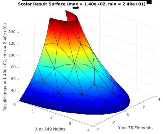
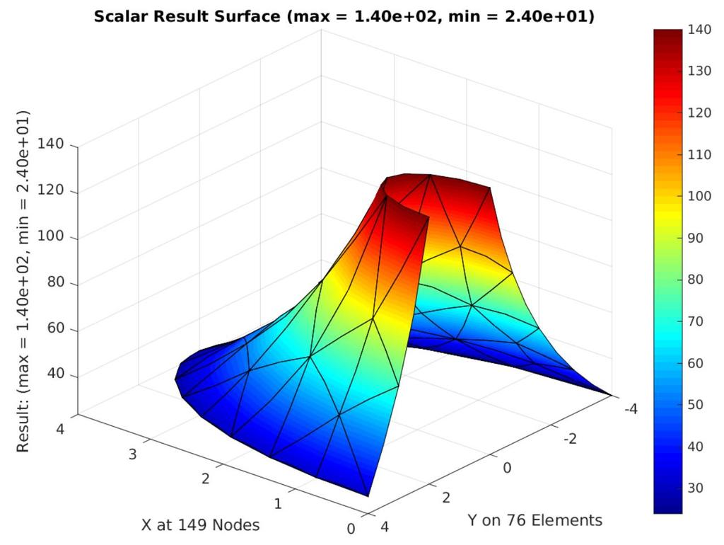
25 through convection on the outer radius (and could be verified by post-processing the edge elements. Figure Partial input files with new element type control data The partial output listing optionally includes the gradient vector and the heat flux vector, from Fourier s law, at each numerical integration point (since control integer show_qp was set to true). The domain volume (for a unit thickness) is also printed as a useful check. Note that the integral of the solution over the area was also given (since integral was true) even though it does not have physical important in heat transfer, but is important in other field problems. The amount of printed output can become huge and is usually suppressed by the user by setting various control integers in the driver script to false (such as debug, echo_p, el_react, integral, show_bc, show_e, show_ebc, show_s). Generally graphical presentation of the results is preferred. Two default plots are the filled colored distribution of the planar temperature (see Fig ) and the temperature represented vertically in a filled color surface plot. The temperature result value plots were produced by scripts color_scalar_result.m and scalar_result_surface.m, which are all called from the field_2d_types.m application software. When running Matlab interactively that type of surface plot can be rotated by changing the eye viewpoint (or manually with the Matlab view command). 25

26 Figure 2.-7 Selected output from the thermal study While temperature is a scalar, the important heat flux is a vector quantity and both its vector display and its contoured magnitude should be displayed. The heat flux data are not available until all of the quadrature point results have been computed and the application closed. Those data are saved to the standard output file el_qp_xyz_fluxes.txt. After termination of the application the script quiver_qp_flux_mesh.m is run to plot the vectors using the Matlab function quiver, and the results are shown in Fig Matlab provides the contour function. However, it expects to operate on a rectangular grid of values. When given values at unstructured node point or quadrature point locations Matlab fits a rectangular grid over the shape and least square fits contours on that regular grid. For a finite element irregular mesh that means that often the contours extend to regions outside the mesh boundary. Also, the least square fit values are often less accurate near rapidly changing FEA values But its use is simpler that writing a contour script for all element types provided herein. To support many different applications of the FEA library the author developed a directory (MatlabPlots) with hundreds of specialized plotting scripts that read the standard input files and 26

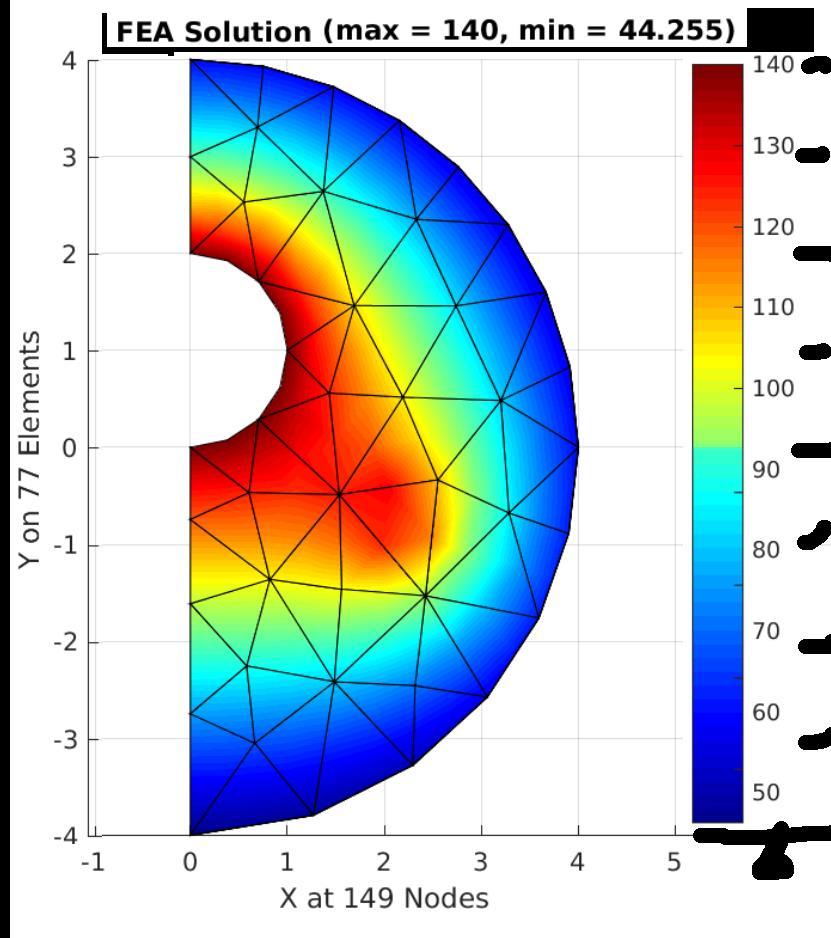
27 Figure 2.-8 Temperature values in a symmetric cylinder 27

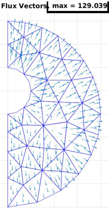
28 Figure 2.-9 Heat flux vectors in a symmetric cylinder Figure 2.- Approximate contours of cylinder temperature and heat flux 28

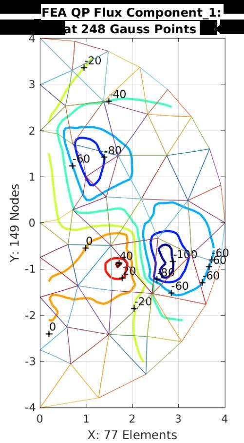
29 standard output files to produce a graphical output. The scripts contour_result_on_mesh.m and contour_qp_flux_on_mesh.m produced the smoothed contour plots given in Fig It is not unusual for a planar part to have a heat source or convection region on part of its surface in addition to on its edges. The current application allows for such face elements too. Let the previous conduction region of element 3 also have a normal heat flux of 5 W cm 2. To include that normal heat source in the previous mesh just append a type 3 element (77) that shares the same nodes as the conduction element (3). Only three lines change in the standard input files, as indicated in Fig The inflow heat flux element location is shown in Fig (plotted by script color_selected_elements.m) as lying on the face of conduction element 3. To include face convection on part or all of the planar area is changed in a similar fashion. That face heat flow warms up the temperature of its surrounding area and changes the overall heat flux magnitude and directions as illustrated by the approximate contours and new heat flux vectors in Fig Those figures should be compared to the prior results like Fig The change in the temperature along the symmetry plane (from script result_on_const_x.m) is shown in Fig Figure 2.- Data changes (arrow) to introduce an area of inward heat flux on a face Figure A type 3 normal heat source element (77) on the conduction face (3) 29

30 Figure 2.-3 New temperature ( ) and heat flux (W m 2 ) from heat source 3

31 Figure 2.- Symmetry axis temperature before (left) and after normal face heat input Example 2.- Given: An 8 by 8 isotropic square has an internal rate of heat generation of Q = 6. The material thermal conductivity of k = 8. Determine the temperature distribution if the sides have a constant EBC temperature of θ = 5. Determine the heat flux vector in each element. Solution: Use one-eighth symmetry and four right angle linear triangular elements as shown below. When all elements have their connectivity listed with the right angle corner being second, all the element matrices (from Table 2.7-2) are the same with S e = [ 8 ] and c et = [ ]. Assembling the system conduction matrix gives:

32 S = 8 [ + ] [ 8 ] + 8 [ + ] [ 8 ] = (8 + + ) ( ) ( ) ( ) [ ( ) S = [ 8 and assembling the heat source vectors gives c = + { + + = } 32 ( ) 8 ( + + 8) ] ] 2 2, and the reaction terms are c R = q 2 { } q 5 { q 6 } The first three rows and columns are the independent ones, and columns, 5, and 6 are multiplied by the EBC value (5) and subtracted from the right hand side to give c EBC = 5 { So the system equations and the unknown temperatures are θ } = { 2} 8.75 [ 6 8] { θ 2 } = { 2} + { 2}, { θ 2 } = { 7.75} 8 6 θ 3 2 θ θ

33 The nodal reactions (outward heat flows) are obtained from the last three rows of the system now that all temperatures are known: 8 [ 8 6 ] q q = { 2} + { q 5 }, { q 5 } = { 29} 5 q 6 q 6 5 { 5 } Of course, the sum of the reactions -8 is equal and opposite to the sum of the sources. Example 2.-2 Given: For the previous temperature calculation of Ex. 2.2-, determine the gradient vectors and heat flux vectors in each element. Solution: To determine the heat flux vectors it is necessary to post-process each element. The post-processing steps are the same as in the prior one-dimensional examples; just the array sizes are bigger. This requires a loop over each element where the local solution results, local node coordinates and element properties are gathered. The locations must be selected for doing the calculations. The guideline is to select the quadrature locations that would integrate the element conduction matrix. Here, that would be a one-point rule, (r = /3, s = /3), which coincides with the geometric centroid of the element. For the linear elements the temperature gradient, and thus the heat flux, are the same everywhere in an element. That means that the heat flux is discontinuous at the element interfaces (as it is for all C elements). To obtain accurate results for the heat flux a very fine mesh must be utilized. For the first element, the element s node connections are [ 2 3], and the gathered temperatures are θ et = [ ]. At the first integration point q = the interpolated physical coordinates are x q = [ 3 3 3]x e =.333. Likewise, y q =.667. The gradient of the solution is θ = B e (r q, s q )θ e and at point is θ θ = { } = θ 2 [ ] θe = { } The heat flux at the point is defined by the Fourier Law q = q = κ θ, and here the constitutive matrix is diagonal with k = 8 values. The heat flux vector is q = {. 6.5 } Example 2.-3 Given: A conducting square has two adjacent edges subject to an inflow heat flux of q n. The other two edges are held at constant temperature. The dimensions and properties are shown below. Determine the temperature distribution estimate using a single element. Solution: For the conduction region select a four-node bilinear rectangle, with the nodes numbered CCW. For each NBC select a compatible line element with two-nodes. The connection list is tabulated: 33 Element Type Node_ Node_2 Node_3 Node_

34 Figure 2.-5 A square with two EBC and two NBC edges In this case, the line element connections are padded with zeros because Matlab requires all read arrays to have a constant number of columns. For general two-dimensional field problems it is allowed to mix triangular (Type ) and quadrilateral (Type 2) area conduction elements. Both of those have lines as their edges. A line can be subject to a NBC with a known normal flux (Type 3) or to a Mixed NBC (Type ). The conduction matrix is known (from Table 2.7-2) as: S e = B e T κ e B e da and for an isotropic material k = K x = K y on a square L = L x = L y it simplifies to A e S e k L = 6 L [ ] On an edge with a NBC of the type that k Θ n = q n the boundary source vector is c q b = H bt q n L b dl On the edge the four area interpolations H e reduce to the two line interpolations H b : H e (r =, s) H b (s) = { s s } That is the same integral developed previously for line elements with a constant source, namely c b q = q n L b t b { 2 } where the L b t b is the area over which the heat flux per unit area enters the domain. Here, the thickness (normal to the area) of the edge is taken as unity. The system equations are, like before, S Θ = c NBC + c EBC The flux resultant, c q b, over the two line elements are assembled to give the resultant NBC source 3

35 c NBC = 2() 2 { } + The sum of those coefficients shows that 6 units of heat entered the body. The reactions entries are not known until the EBC DOFs are identified. Here, nodes, 2, and have EBCs of Θ =, so c EBC T = [R R 2 R ] are the reaction heat flows to be determined. Thus, () 6() [ 2 2 Θ R 2 2 Θ ] { 2 } = { R } + { 2 } Θ 3 2 Θ R Only row three is independent for finding the temperature. Moving the EBC terms to the right side []{Θ 6 3} = {8} + {} Θ { 2 } Θ 6 2 { } Θ 6 { }, Θ 6 3 = 2 Now use the remaining rows to determine the reactions: 2 () [ 2] { 6() 2 2 R R } = { } + { R 2 }, { R 2 } = { 6} R R 6 As expected, the sum of those terms show that 6 units of heat flowed out of the body at the EBCs in order to maintain them. Example 2.- Given: Graph the previous temperature results along the diagonal -3. Solution: First, the interior temperature values must be found. Of course, that is done by interpolating between the know temperatures. In unit coordinates Θ(r, s) = H(r, s) Θ e. From the summary or Matlab interpolation scripts the Q quadrilateral element interpolations are: H(r, s) = [( r s + rs) (r rs) (rs) (s rs)] = [H H 2 H 3 H ]. However, only Θ 3 is not zero so the temperature surface is approximated as Θ(r, s) = H 3 Θ 3 = rs Θ 3 = 2 r s which can be easily contoured by Matlab (the surface is a hyperbolic paraboloid). The diagonal line is given by s = r so the in that direction Θ diag = 2r 2. Thus the approximate temperature estimate increases quadratically from corner one to corner 3. Of course, this is a crude estimate because only one DOF was utilized. 2. Torsion of non-circular shafts: Today it is common to encounter non-circular shafts, like thin walled extruded members, and large torsional members. The behavior of any torsional member is directly related to a geometric parameter, J, called the torsional constant which is proportional to the polar moment of inertia of its cross-section, and its material shear modulus, G. The product of the two, GJ is called the torsional stiffness of the shaft. The simple expressions for the shear stresses and deflections in circular were derived about 8. But the failures of shafts with non-circular cross-sections continued to be a common problem for another half a century. Then Saint-Venant, circa 855, introduced a warp function that reduced the problem to solving a second order partial differential equation over the cross- 35

36 sectional area. In 93 Ludwig Prandtl published a simpler solution by introducing the concept of a stress function that reduced the problem to solving a simpler second order partial differential equation. That PDE is the same as the one that determines the shape of soap film surfaces. For many decades, before digital computers, the stresses in non-circular shafts were determined by very careful experimental measurements of the deflections and slopes of inflated membranes. Prandtl s equation is a form of the Poisson s equation and is easily solved for any shape by finite element analysis. Prandl s equation for the stress function, φ(x, y), of an isotropic elastic shaft is ( φ ) + ( φ ) + 2θ = (2.-) G x G y where G x and G y are the orthotropic shear moduli of the material and θ is the angle of twist per unit length about an axis parallel to the shaft. The most common case is where the shaft is an isotropic material where G x = G y = G. The essential boundary condition is that the stress function is a constant on each peripheral boundary curve. When there is only one exterior boundary curve the stress function is set to zero. When the shaft has interior boundaries around a hole or a different material (a different G) its constant value is not known and must be obtained by placing a constraint on the solution that computes the required additional constant(s) as part of the solution. In a FEA study that is accomplished by the use of a different material filling the closed interior curve, or by a sophisticated algebraic constraint (usually known as repeated freedoms, which is not covered herein) applied to all nodes on that interior curve. From the finite element point of view the stress function is different because it does not have a physical meaning, but its integral does, and its gradient components do have physical importance. Let the cross-sectional area lie in x-y plane. Then the angle of twist per unit length, θ, is about the z-axis as is the torque (couple) reaction, T, required to maintain that angular displacement. At all points in the boundary there are only two non-zero components of the stress tensor; namely the shear stress components, τ zx and τ zy, acting parallel to the x- and y-axes, respectively (see Fig. 2.-5). The shear stress components are orthogonal to the gradient of the stress function: τ zx = φ and τ zy = φ, τ max = τ 2 zx + τ 2 zy (2.-2) Figure 2.-6 Shaft shear stress components due to torsion The maximum shear stress at the point can be plotted as the surface stress vector (σ i = 3 j= σ ji n j ), which in this special case lies in the flat plane of the cross-section. From the membrane analogy, the slope of the bubble is maximum at, and perpendicular to, the boundary curve. That means that the maximum shear stress will occur at a point on the boundary. At an exterior corner the shear stress goes to zero. But, any sharp reentrant corner is a singular point where the shear stress, in theory, goes to infinity. Therefore, any reentrant corner should have a 36

37 curved fillet that lowers the shear stress to an allowable material limit. For and area enclosed by a single boundary the points of maximum shear stress are at locations on the boundary which touch the largest inscribed circle; such as the shapes in Fig Figure 2.-7 Points of maximum torsional shear stress The externally applied torque, T, is defined by twice the integral, over the cross-section, of the stress function: T = 2 φ(x, y) d (GJ)θ. (2.-3) In practice however, we generally know the applied torque, T, and not the twist angle that appears in the differential equation. Thus, a unit twist angle (θ = ) is assumed and the finite element model is solved for the stress function. Then the integral of the stress function is computed to give the corresponding torque, say T fea. Then, all of the stresses and the angle of twist are scaled by the ratio T actual T fea to obtain the results that correspond to the actual applied torque. Two important analogies are useful in the calculation of torsional shear stresses because they share the same differential equation. They are the soap film membrane analogy and the thermal analogy (considered above). Their differential equations are: soap film membrane: (N w x ) + (N w y ) + P = heat conduction: (k x ) + (k x ) + Q = The thermal conduction analogy is important because it is available in most commercial FEA programs, while torsional analysis of a non-circular section is not specifically identified as an analysis option. To use heat conduction for torsion analysis just change the meaning of its data (and edit the headings of its plotted results). The temperature, u, becomes the stress-function, φ. The input rate of heat generation becomes twice the rate of twist, Q = 2θ, and the thermal conductivity is input as the reciprocal of the shear modulus, k x = G x. Then the temperature gradient vector, u, has the magnitude of the shear stress, but its direction is off by 9. The soap film membrane analogy is important because it lets an engineer visualize the shear stress distribution over the cross-section of the shaft. In a soap film membrane inflated over a 37

38 boundary with the same shape as the torsional bar the membrane deflection corresponds to the value of the stress function, w = φ, and its inflation pressure is proportional to the angle of twist, P = 2θ, The membrane force per unit length is the reciprocal of the shear modulus, N x = G x. The slope of the soap film is proportional to the shear stress at the same point, but the resultant shear stress acts in a direction perpendicular to that slope. On the bounding perimeter the slope of the membrane is perpendicular to that curve; thus, the shaft shear stress is tangent to any closed bounding perimeter curve. The membrane analogy makes it possible to visualize the expected torsional results for the two most common shapes of a circular and a rectangular cross-section. For a circular bar the shear stress is zero at the center, increases radially, and is maximum and constant along its circular boundary. Therefore, the circular shaft has contours of shear stress are concentric circles. The distribution of shear stress is more complicated for a rectangular cross-section. It is also zero at the center point, but the maximum shear stress occurs on the outer boundary at the two midpoints of the longest sides of the rectangle; while zero shear stress occurs at the corners of the rectangle (why?). Two typical classes of the torsion of non-circular shafts will be illustrated. First consider a symmetric aluminum circular shaft (G = 3.92e6 psi) with an eccentric circular hole. Had the hole been at the center, the problem would be the classic one dimensional solution where the shear stress is directly proportional to the radius. The presence of the hole means that the condition of an unknown constant stress function value along the interior boundary curve must be enforced, or tricked into being satisfied. One trick is to fill the empty with something like air which has a shear modulus of approximately zero compared to aluminum. That is, insert elements into the hole space and make the fake material modulus or 5 times smaller than that of the surrounding material. The shape is shown on the left of Fig. 2.-8, with R = in., d = in., r = in. along with the half symmetry upper half of the domain that was meshed with an unstructured group of six node curved triangular elements (T6). The center hole region was filled with four fake material (type 2) elements (63-66). The fake type 2 elements are shown in an exploded view in Fig. 2.-9, and the EBC values applied to the outer boundary are shown in Fig Figure 2.-8 Eccentric shaft and half-symmetry mesh with two element types 38

39 Figure 2.-9 The type 2 elements Figure 2.-2 Essential BC locations and values There is a matrix algebra way to enforce the requirement that all of the nodes on the boundary of the interior hole must have the same (unknown) constant value. That type of constraint is common in electrical engineering but rare in mechanical engineering, thus it is not included here. Instead, the trick of inserting a fake material having a shear modulus that is ten thousand times smaller was used. A unit angle of twist was input along with the true and fake shear moduli. The application script field_2d_types.m, which is intended for planar scalar field solutions, was utilized to calculate the stress function and the shear stress components. The stress function value is shown with colored values and as approximate contours in Fig Figure shows carpet plots over the cross-section where the vertical coordinate is the stress function value. Occasionally a graph of the results along a selected line is useful, and the stress function is plotted along the symmetry line in Fig Figure 2.-2 Stress function distribution and approximate contours 39

40 Figure Stress function as carpet plots The main quantities of interest are the magnitudes and directions of the resultant shear stress vector at points on the surface. Approximate contours of the maximum shear stress are given in Fig The theory shows that the maximum values occur at points on the boundary. The FEA stress vector plots are most accurate at the Gauss points which usually do not fall on the boundary. However, as the number of quadrature points is increased some of those points always get closer to the boundary. Therefore, torsion is an application where it can be useful to increase the number of integration points beyond the number needed to integrate the element matrices, at least in a few selected elements. Here, seven quadrature points were used to enhance the stress vector plot even though only four points were needed to integrate the element matrices. The shear stress vectors for this domain are shown in Fig In this case, the topmost element in the left corner contains the maximum shear stress. Figure Edge function values Figure 2.-2 Approximate max shear contours

41 Figure Maximum shear stress distributions To obtain the above results and figures the control integer torsion was manually set to true to activate the few alterations required for this class of solution. They include reading G x and G y as properties, but converting them to k x = G x and k y = G y for calculating the equivalent conduction matrix. The control integer color was manually set to true to produce color area and carpet plots of the stress function with color_scalar_result.m and scalar_result_surface.m which are on the left of Figs and The stress function colored and contoured values show that the hole acted like an enlarged center hole. As such a hole approaches the outer radius its effect on the shaft becomes more pronounced (as standard stress concentration tables suggest). The standard output text files, node_results.txt, node_reaction.txt, and el_qp_xyz_fluxes.txt, are always saved upon completion of the analysis. The other graphs, contours, carpet plots, and resultant shear stress vectors were created after the execution was completed by selecting scripts from the supplied Matlab_Plots directory which only use the data in the standard input and output files. Those scripts were the graph from the result_on_const_y.m, the (color) contour_result_on_mesh.m, and contour_qp_flux_on_mesh.m, the (color) result_surface_plot.m, and the hidden_result_surface.m line plot. The next class of torsional analysis is that of open thin-wall members which are typical of extrusions in metal and plastic. They are called open if the section never closes back on itself, otherwise they are called thin-walled tubes. The two types of thin walled members have very different shear stress distributions. The current open extrusions have zero shear stress generally

42 along the center of the thickness and maximum shear stress at the outer thicknesses, but running in opposite directions. In other words, along a line perpendicular to the thickness the shear stresses are equal but opposite relative to the line mid-point and thus form a small torque, but no net force. At free ends of a leg of the extrusion the shear stress is tangent to the end. Figure shows a typical extrusion with half-symmetry. The symmetric section was meshed with curved nine noded quadratic Lagrange quadrilaterals with EBC values of zero on the perimeter excluding the lie of symmetry (see Fig ). Figure A symmetric thin-wall channel extrusion subject to torsion The torsion option in the application field_2d_types.m was utilized again to obtain the solution. It gave the stress function distribution in Fig The steep gradient at the re-entrant corner is hard to see there, but will become apparent. Figure shows that the maximum stress function, and thus the minimum shear stress, occurs on the symmetry line near where the centerlines of the two legs intersect. The resultant shear stress vectors were evaluated at each of the nine numerical integration points in each quadrilateral and are shown in Fig Along the thin arc it is easy to see that the shear stress is maximum along the perimeters, but act in opposite direction on the other side perimeter. The top right of that figure shows the shear stress approaching zero at the exterior corners, flowing parallel to the free end, and reversing direction to flow along the inner perimeter. The dashed arrow indicates the singular point at the re-entrant corner where the shear stress in theory goes to infinity. The Gauss points are offset from the corner and thus do not pick up that value. Any small fillet there will remove the mathematical singularity. 2

43 Figure Half-symmetry quadratic quadrilaterals mesh and EBC points Figure Stress function colored values 3

44 Figure Stress function values on symmetry line and arc center Figure 2.-3 Stress function carpet plot

45 Figure 2.-3 Maximum shear stress vectors with a singular point The thermal analogy will exactly solve torsion problems if the user creates a custom material where the thermal conductivity is the reciprocal of the shear modulus, etc. Here, any constant conductivity and constant heat generation rate will show the same qualitative results. The commercial SolidWorks finite element system was used for this analogy. Figure 2.-3 shows a thermal study mesh consisting of quadratic triangles (T6) refined around the singular point, the temperature (stress function) contour, and a temperature gradient (shear stress magnitude) contour. The temperature gradient (shear stress magnitude) was graphed along the straight leg to the singular point, and then away from that point along the arc. At the two end corner points the 5

46 shear stress (temperature gradient) vanishes, then it approaches a constant along the perimeter unit the singular point is where it rises toward infinity in Fig The shear stress directions are visualized as rotating the temperature gradient vector by 9 degrees (see Fig ). Figure 2.-3 Thermal analogy mesh, stress function, and shear stress magnitudes Figure Thermal analogy graph of the shear stress on the straight leg and arc Figure The temperature gradient is orthogonal to the shear stress 6

47 The third class of torsion analysis is where the shaft is a thin walled closed tube. Then, the shear stress flows around the perimeter with a constant value that is independent of the material modulus. For a tube with a constant thickness, the mechanics of materials theory gives the constant shear stress as τ = T 2At where t is the tube thickness and A is the area enclosed by the median line of the thickness of the tube. For multiple wall thicknesses this becomes slightly more complicated theory. For a closed tube with multiple closed cells another mechanics theory is available to predict the shear stress flow distribution. The assumption of constant shear stress through the wall thickness is reasonable but not exact. To illustrate that consider the thin closed aluminum tube shown in Fig There the dashed centerline curve denotes the perimeter used in the elementary theory to calculate the reference area, A. The tube was modeled with a structured mesh of quadratic nine noded quadrilateral elements, including nine fake interior elements to account for the unknown EBC value around the tube interior perimeter. The mesh was created with a structured mesh generator that created the condensed data summaries in Fig Again all of the nodes on the outer perimeter were assigned the EBC value of zero. Figure 2.-3 A closed thin wall tube with piecewise constant thicknesses For a torque of 3, kpa-m the mechanics of materials theory for this geometry predicts a constant shear stress in the 3 mm thick leg of 93. MPa and a value of 55.8 MPa in the walls with a thickness of 5 mm. The torsion differential equation was solved for this tube section. The graph of the stress function horizontally across the tube at the middle of the open segment is shown in Fig It shows that the value across the right wall has a nearly constant slope (shear stress value) while the section through the thicker left was a slightly changing slope. The distribution of the shear stress vectors for the full domain is in Fig and supports the reasonable assumption of approximate constant shear flow in each constant thickness section. 7

48 Figure Compressed data for the structured tube mesh Figure The stress function values midlevel across the tube opening 8

49 Figure Shear stress vectors for the thin walled closed tube To compare to the elementary theory the average shear stress was calculated in the elements in the middle of the vertical legs. From the lists in Fig they are elements 37, 38, and 39 in the 5 mm wall and 3,, and 5 in the 3 mm wall. The averages of the quadrature point values in those elements were 55.7 MPa and 99.6 MPa. Comparing to the mechanics of materials solutions of 55.8 MPa and 93. MPa the simplified solution is only off by 7%. 9

50 2.5 Axisymmetric fields: The governing equation, (2.-), can be transformed into cylindrical coordinates of (R, θ, Z). The gradient vector components are u = [ R r θ Z ]T (2.5-) and Fourier s Law for the heat flux vector remains the same. The diffusion term in (2.-) becomes ([κ] T u(r, θ, Z, τ)) = (Rκ R R RR ) + (κ R R 2 θ θθ ) + (κ θ z zz ) Z for an orthotropic material, and a differential volume is dv = R dr dθ dz. Then the solid is a body of revolution and the source terms and boundary conditions are independent of the angular position, θ, then θ = and the problem becomes a two-dimensional axisymmetric study. For a model PDE of the form multiplying by the radius gives Comparing to the planar PDE R (R k R R ) + (k R Z Z Z 5 ) + T u(r, Z) + Q(R, Z) = ({R k R R} ) + ({Rk R Z Z} ) + {R T}u(R, Z) + {R Q(R, Z)} = (2.5-2) Z (k x ) + (k y ) + T u + Q(x, y) = the axisymmetric model can be viewed as a planar model where the constant thickness form I = u(x, y) [ (k x ) + (k y ) + T(x, y)u + Q(x, y)] t(x, y) da = A is simply replaced by the variable thickness of the volume of revolution, t(x, y) = 2π R to give I = u(r, Z) [ (k R R ) + (k R Z Z ) + T(R, Z)u + Q(R, Z)] 2π R da = (2.5-3) A Z In other words, the planar analysis program can have a control integer, say axisym, which switches the evaluation of all of the element matrices to an axisymmetric analysis by branching to utilize the variable thickness (circumference) at every numerical integration point. This means that the prior integral matrix definitions are all simply multiplied by 2π R which usually means that the number of quadrature points must be increased by. In practice, it is inefficient to multiply by 2π millions of times while doing the numerical integration over a complicated mesh and then having them all cancel out after assembly of the system. For example, the only change in the source vector term, c Q e, due to the volumetric rate of heat generation, Q, is c e Q H et Q e d = e H et Q e R da (2.5-) A e

51 Likewise, the only change from the two-dimensional diffusion matrix to the axisymmetric case (per radian) is including the radial position when conducting the numerical integration and increasing the number of quadrature points: EXAMPLE S e κ = B et κ e B e d = e B et κ e B e R da. (2.5-5) A e 2.6 Three-dimensional fields: All of the planar problems discussed above are easily extended to three-dimensions, and the supplied Matlab scripts will execute such problems just by changing the number of physical space dimensions to three (n s = 3), utilizing the eight node hexahedral (brick) element by setting the parametric element space to three and the number of nodes to eight (n p = 3, n n = 8), and selecting the correct number of integration points, which is usually 2 3 =8 but may be 27. The size of the constitutive matrix, E e, and the operator matrix, B e, must be increased to three (n r = 3) by adding the z derivative of the interpolations as its third row. Of course, additional elements can be added to the element library. However, most threedimension problems are better solved with commercial software simply because they have automatic solid element mesh generators and offer several good graphical post-processing tools. As a minimal validation of the three-dimensional Poisson solver a patch test was run with six eight-node trilinear hexahedral elements using EBS that make the gradient vectors components everywhere be (2,, ). Figure 2.6- Mesh for three-dimensional Poisson equation patch test 5

52 Figure Linear spatial solution and selected constant flux vectors from patch test 52