2. Polynomial interpolation

Transcription

1 2. Polynomial interpolation Contents 2. POLYNOMIAL INTERPOLATION TYPES OF INTERPOLATION LAGRANGE ONE-DIMENSIONAL INTERPOLATION NATURAL COORDINATES* HERMITE ONE-DIMENSIONAL INTERPOLATION* LAGRANGIAN QUADRILATERAL ELEMENTS LAGRANGIAN TRIANGULAR ELEMENTS SERENDIPITY QUADRILATERALS HIERARCHICAL INTERPOLATION* SUMMARY AND NOTATION EXERCISES INDEX Types of interpolation: Three types of polynomial scalar interpolation will be used in most of the applications given later. The most common ones (Lagrange interpolation and Serendipity interpolation) use only the value of a function at every node on the element. In onedimension, adding another node simply raises the polynomial degree by one. Such elements are usually employed to solve second order partial differential equations (PDEs). A third approach, Hermite interpolation, uses the value of a function and its spatial derivative(s) at every node on the element. In one-dimension, when using the function and just its slope, adding another node raises the polynomial degree by two. Such elements are usually employed to solve fourth order PDEs. When simulating plates or shells, the nodal degrees of freedom can be extended to include the curvature (second or higher derivatives) at the nodes. These types of interpolations are classified mathematically by the level of continuity between adjacent regions of interpolation. A function is said to be C n continuous when the function (n = 0) through its n-th derivative is continuous. All of the interpolation functions used here are C on the element interior, but have very low continuity at their boundary with another element. The Lagrange interpolation and Serendipity interpolation functions only have their values (zero-th derivative) shared at the boundary of an adjacent element. Therefore, they are referred to as C 0 elements. The Hermite family has the function and at least the first derivative(s) shared at the boundary with an adjacent element. Therefore, they are at least C 1 elements, but can be C 2 or higher in their continuity. In one-dimension it is easy to create C n elements, but it is very difficult to create them in two- and three-dimensions (while retaining local support). Hermite C 1 interpolation is typically used on 4-th order PDEs (like beams and plates) and Hermite C 2 interpolation is typically used on 6-th order PDEs (like ideal centrifuge flows). 1

2 It is not necessary to require the same number of unknowns at each node, but that common approach will be followed in this book. All of the interpolation functions to be used here have been known for at least fifty years and can be found in handbooks on finite element analysis or handbooks on mathematical analysis. However, experience shows that students do not find them obvious. Therefore, several of them are derived herein and Matlab symbolic scripts are given to illustrate how they can be derived in general. 2.2 Lagrange one-dimensional interpolation: Applying Lagrange interpolation requires estimating the values of a function u(r) based on locations r k for k = 1,, n at which the values u k are known. In this book, only equally spaced intervals, r, will be employed in the parametric space. The expressions for the finite element interpolations are well known and will generally be given without proof. For completeness, the one-dimensional (n p = 1) quadratic C 0 interpolation function, in unit coordinates will be derived here. Consider a three-node quadratic line element (n n = 3). A complete quadratic polynomial in one-dimension has three constants. In the unit coordinate space ranging from zero to one, the three equally spaced parametric locations are r 1 = 0, r 2 = 1 2 and r 3 = 1, and the non-dimensional measure of the parametric range is λ = (r 3 r 1 ) = 1. Let the polynomial data fit be u(r) = c 1 + c 2 r + c 3 r 2 = [1 r r 2 ] { } [P(r)]{c} = P(r)c = c T P T (r) c 3 Where the row matrix P(r)is the assumed polynomial and c denotes a column matrix of mathematical constants. A quadratic interpolation using three data-values is shown in Fig (where the interior node x 2 does not have to be L/2, but it usually is). c 1 c 2 Figure A quadratic line interpolation between three values The solution could be completed using these mathematical constants, but engineers prefer to relate the solution to the actual solution physical values. To relate the three constants to physical values note that there is an identity at each local parametric node: c 1 u(r k ) u k = c 1 + c 2 r k + c 3 r 2 k = [1 r k r 2 k ] { c 2 }, 1 k 3 c 3 Evaluate this identity at the three uniformly spaced parametric locations (r 1 = 0, r 2 = 0.5, r 3 = 1), where the three function values (u 1, u 2, u 3 ) occur, on at each node. These three identities can be written together to yield a matrix identity: 2

3 u(r 1 ) u c 1 { u(r 2 )} { u 2 } = [ ] { c 2 }, u(r 3 ) u c 3 or u e = G c where u e denotes a column matrix containing the physical value of the solution at the nodes. Each row of the square matrix, G, is just the polynomial row matrix evaluated at the local node coordinates: P(r 1 ) 2 1 r 1 r 1 G [ P(r 2 )] = [ 2 1 r 2 r 2 ], P(r 3 ) 2 1 r 3 r 3 Here, G is non-singular and its inverse is computable, and it lets the initial constants, c, be replaced by the spaced physical values, u e : c = G 1 u e = [ 3 4 1] u e Eliminating the non-physical constants in favor of the interpolation data yields the interpolation equations, H(r) in finite element analysis: u(r) = P(r) G 1 u e H(r)u e. These functions are also known as the shape functions because in structural analysis they actually describe the shape of the deformed member. Note that the interpolation (shape) functions are formed from an assumed polynomial, geometrical data about the local non-dimensional placement of the nodes, and the physical values at those nodes: u 1 u(r) = [1 r r 2 ] [ 3 4 1] { u 2 } u 3 u 1 u(r) = [(1 3r + 2r 2 ) (4r 4r 2 ) ( r + 2r 2 )] { u 2 } u 3 u 1 u(r) = [H 1 (r) H 2 (r) H 3 (r)] { u 2 }. (2.2-1) u 3 Since u(r) is a scalar quantity it is the same as its transpose: u(r) = u(r) T = u et H(r) T. Also, since the interpolation functions, H(r), are dimension-less the approximation u(r) takes on the units of the item being interpolated, u e. Having made this selection for the parametric spatial form, the parametric local derivative is also known: u r H(r) (r) = u e = [ H 1 r r (r) H 2 r (r) H u 1 3 r (r)] { u 2 } u 3 u r (r) = [( 3 + 4r) (4 8r) ( 1 + 4r)] { u 1 u 2 u 3 } (2.2-2) 3

4 since the derivative of any matrix contains the derivative of each of its terms. The above quadratic interpolation functions and their parametric local derivatives can easily be obtained using symbolic calculations. The symbolic Matlab script equivalent to the above derivation is given in Fig , while its output is given in Fig (Note: the latest releases of Matlab have discontinued the use of the keyword positive and just uses real.) This quadratic interpolation also includes the subset for a linear interpolation or a constant value. For a result that is linear, u 2 = (u 1 + u 3 )/2 and the above quadratic simplifies to a linear interpolation, which depends only on the two end values, namely u(r) = (1 3r + 2r 2 )u 1 + ((4r 4r 2 ) u (4r 4r 2 ) u 3 2) + ( r + 2r 2 )u 3 u(r) = (1 3r + 2r 2 + 2r 2r 2 )u 1 + (2r 2r 2 r + 2r 2 )u 3 u(r) = (1 r)u 1 + ru 3 = [(1 r) r] { u 1 u 3 }. However, if we wanted just a linear approximation it is more common just to use a two node element, as in Fig , and denote its interpolation as u(r) = [(1 r) r] { u 1 u 2 } = [H 1 (r) H 2 (r)] { u 1 u 2 }. (2.2-3) Likewise, if all the values are the same constant then the quadratic interpolation must simplify to that constant. For that to be true, all the interpolation functions must sum to unity for any and all values of r: k H k (r) 1 (2.2-4) 4

5 Figure Matlab symbolic derivations of the quadratic line interpolation functions To illustrate that (convergence) requirement use the constant data v = u 1 = u 2 = u 3. Then the quadratic interpolation degenerates to u(r) = (1 3r + 2r 2 )v + (4r 4r 2 )v + ( r + 2r 2 )v, or simply u(r) = v, as expected. These two simplifications of a quadratic interpolation are also confirmed by the Matlab symbolic calculations in Fig Since Lagrangian interpolations, H k, sum to unity at any local point their values can be thought of as the percent of u 1, u 2, and u 3 that contribute to the total interpolated value of u (r). Since this interpolation approach exactly matches the data, u k, at the control points, r k, this is a Lagrangian interpolation. In this book, linear through cubic C 0 Lagrangian polynomials will be applied to first and second order PDEs. Cubic through quintic C 1 Hermite polynomials will be utilized in fourth order PDEs. In general, a Lagrange interpolation function evaluated at its control point will have a value of unity and it will be zero at any other control point: H k (r j, s j, t j ) = { 1 if j = k 0 if j k δ jk (2.2-5) 5

6 Figure Output for line quadratic interpolation (L3_C0) Figure Linear line element interpolation functions (L2_C0) The process so far only gives the interpolation and parametric derivative of the interpolated quantity. Differential equations utilize the physical (x) derivatives of u(r), and once u(r) is known it is usually necessary to find its gradient, u x = u r r x. In order to do that, the physical coordinate, x, must be defined in terms of the local parametric coordinate. Then the nodal u k values are simply replaced by nodal x k values. The above quadratic interpolation was described as interpolating a solution value, but it could be applied to interpolating anything that is associated with the three nodes on the element. For a straight line element only the two end point coordinates are needed for the geometry. A linear geometry interpolation is obtained by having (2.2-3) interpolate the end coordinate values instead of solution values: 6

7 x(r) = [(1 r) r] { x 1 x 3 } = x 1 + r(x 3 x 1 ) = x 1 + r L (2.2-6) where L is the physical length (or measure) of the element. This form automatically occurs (as seen in Fig ) when the interior node is placed exactly at the mid-point of the physical length. That is almost always the preferred way to describe the geometry. The unit coordinate version of the 1D linear, quadratic, and cubic C 0 Lagrangian interpolation functions are given in Matlab script Lagrangian_1D_library.m shown in Fig Figure Constant and linear results are included in quadratic interpolation Mathematical terminology defines that a function is C n continuous when the function and its first n derivatives are continuous. Therefore, the prior Lagrangian elements are called C 0 on their boundaries, but are C on the interior of the element. Several C 0 interpolation functions for 1D, 2D, and 3D elements are given in the Matlab script el_shape_n_local_deriv.m which is also included in the general library of finite element scripts. A subset of the one-dimensional interpolations is included in Lagrangian_1D_library.m. Such a function accepts a numerical 7

8 Figure Placing interpolation functions in a script for a library of 1D elements value for the parametric coordinate(s) and returns numerical values of the interpolation functions and numerical values for the (rectangular array) of local derivatives of those interpolation functions. It will be shown later that such scripts are necessary to automate the numerical integration processes almost always needed in a finite element simulation. In general, for straight line elements using equal physical space increments between the nodes causes this linear mapping between parametric and physical spaces. For this common special case, x r = L and the physical derivative of u(r) in a straight element is u = u x r r = u x r 1 L. (2.2-7) Example Given: A four-node cubic line element (L4_C0), with equal node x-spacing, has temperature nodal values of u 1 = 2, u 2 = 3, u 3 = 2, and u 4 = 1. The physical coordinates are x 1 = 2 cm, x 2 = 4 cm, x 3 = 6 cm, and x 4 = 8 cm, so the length of the element is L = 6 cm. Fill in the element degree of freedom vector, u e, and the element coordinate vector, x e. At local point r = 0.7 find the physical coordinate, x, the interpolated value of u(r), and the physical gradient of the solution, u x. Solution: The element degrees of freedom are u et = [ ] (transposed) and its coordinates are x et = [ ] cm. From or the script Lagrange_1D_library.m the shape functions are: H(r) = 1 2 [(2 11r + 18r2 9r 3 ) (18r 45r r 3 ) ( 9r + 36r 2 27r 3 ) (2r 9r 2 + 9r 3 )] 8

9 The equal spacing of the physical nodes causes a linear geometry mapping. That could be seen by doing the actual multiplication, x(r) = H(r)x e = (2 + 6r) cm = x 1 + L r. So at x(0.7) = 6.2 cm. In practice, the r coordinate is substituted into H to get its numerical values and then the two arrays are simply multiplied: 2 x(r = 0.7) = H(0.7)x e = [ ] { 4 } cm = cm. 6 8 It happens that the u(r) values falls on a parabola, so they are actually quadratic. The cubic interpolation automatically can capture a set of quadratic data, or linear data, or constant. That could be seen by actual multiplication, u(r) = H(r)u e = (2 + 6r 9r 2 ), so at the local point u(0.7) = Again, in practice, the process is automated by just multiplying the numerical values of H and by the nodal degrees of freedom: 2 u(r = 0.7) = H(0.7)u e = [ ] { 3 } = Fig shows the red interpolated u(x) curve for these data. The blue line at the top represents the range of the unit coordinates. The arrows show the interpolated values at the given r value. To compute the physical gradient it is necessary to compute the Jacobian and its inverse. Looking up the local derivatives from the same sources for the cubic gives H(r) r = [( r 27r 2 ) (18 90r + 81r 2 ) ( r 81r 2 ) (2 18r + 27r 2 )]/2 The Jacobian is J(r) = x r = H(r) r x e. If the actual multiplication is done to get the Jacobian as a function of r the result (in this case) is J(r) = 6 cm/1. That is, the Jacobian (matrix) is constant. In practice, this process is automated by substituting the numerical value of r into the expression J e (0.7) = x r = H(0.7) 2 x e = [ ] { 4 } cm = cm/1 r 6 8 The determinant and inverse are J e (0.7) = J e (0.7), and J e (0.7) 1 = r x = 1 6 cm. The superscript e was added as a reminder that element geometry was used. The local derivative is 2 u(0.7) = H(0.7) r u e = [ ] { 3 } = /1. r 2 1 The physical gradient is u(r = 0.7) x = u(r = 0.7) r r(0.7) x = ( ) ( 1 ) = cm. 6 cm Figure shows the interpolated red gradient curve for these data. The blue line at the top represents the range of the unit coordinates. The arrows show the interpolated values at the given r value. This example could be thought of as computing one point on a graph of the solution and 9

10 its gradient. Of course, if the interpolations are done using natural coordinate interpolations the exact same results are obtained. It is often desired to plot such a graph for all the elements at once. The next example shows how to build such a graph for only one element. Example Given: Change the data given in Ex to u 3 = 0, and plot the temperature and the temperature gradient. Solution: The change in the EBC value means that the full cubic nature is active (since the data no longer fits on a parabola). To create the graph it just necessary to loop over the number of points in the parametric domain needed to make the physical domain graph look smooth. At each point in the local coordinate the above example calculations are repeated. The results are shown in Fig A script for creating the graph is given in Fig If the lines for calculating arrays H and DLH were replaced with a call to the library of 1D elements this process would work for any 1D Lagrangian element considered here. Such a script is in the FEA analysis library as script Lib_1D_graph.m. (Think about how you could extent this process to plot all elements in the mesh.) Note that if the given requirement was to plot the magnitude of the heat flux vector then the process would be essentially the same. The material thermal conductivity, K, would have also been input. After the gradient values were computer and stored in its array Fourier s Law would have been applied: q = K u. In other words, the second plot would have its sign changed and its height scaled by K. Example Given: A 90 degree segment of a circular arc of radius 4 cm is modeled by a single four-node line element in order to approximately determine the arc length. Plot the curved element in physical space. Solution: Let the arc center point be at the x, y origin. Then the x- and y-coordinates of the four nodes are x e = [4, 3.464, 2, 0]cm, y e = [0, 2, 3.464, 4]cm To plot this one element, just alter the previous temperature graphing script by replacing the u values with the y-values. The mesh curve is in Fig , and the modified script to plot the curve is in Fig The integer node numbers were added for clarity. 10

11 Figure Using a cubic to exactly interpolate a parabola Figure The interpolated gradient of a parabola 11

12 Figure Graph of a cubic element and its gradient 12

13 Figure A Matlab script to graph a cubic element (L4_C0) 13

14 Figure Plot of a single curved cubic element Figure Script to plot a single curved parametric element BOLD 14

15 2.3 Natural coordinates*: In addition to the above unit coordinate system, much of the finite element literature also utilizes a parametric system set on 1 a 1. Here, this is called a natural coordinate system. The above symbolic process works just as well for deriving the corresponding quadratic interpolation functions in that coordinate system, as shown by the Matlab symbolic script in Fig Of course, the two parametric coordinates are related since r = (a + 1)/2. Therefore, any interpolation function given in one coordinate system is easily converted to the other. The natural coordinate system is popular in part because most of the data required for numerical integration were originally published for such a domain. Figure The Lagrange quadratic line interpolation in natural coordinates 15

16 2.4 Hermite one-dimensional interpolation*: Polynomials that exactly interpolate the data, u k, and one or more of the physical derivatives at the control points, like u k x = u k = θ k, define a C 1 Hermite interpolation. In that case, there are two degrees of freedom at each control point (n g = 2). Hermite interpolation uses a higher degree on mathematical continuity between the elements. Hermite polynomials are at least C 1 on their boundary but also C on the interior of the element. The one-dimensional (n p = 1) three-node (n n = 3) parametric space C 1 Hermite element would have six constants(n i = n g n n = 6) so the polynomial must be of fifth degree. Since the physical slope is included in the control data it is necessary to also define x(r). Since x is a scalar, use the same quadratic interpolation process and set x(r) = H(r) x e. Usually, the physical nodes are also equally spaced. In that case, x 2 = x 1 + L 2 and x 3 = x 1 + L, where L is the length of the region in one-dimensional physical space (n s = 1). Then, the quadratic terms cancel and the geometry mapping is linear x(r) = (1 r)x 1 + r (x 1 + L) = x 1 + rl. Repeating the above process used for the prior C 0 interpolation functions and inverting the resulting 6 6 G matrix gives the three-node quintic Hermite interpolation: u(r) = [u 1 (1 23r r 3 68r r 5 ) + θ 1 (r 6r r 3 12r 4 + 4r 5 )L +u 2 (16r 2 32r r 4 ) + θ 2 ( 8r r 3 40r r 5 )L +u 3 (7r 2 34r r 4 24r 5 ) + θ 3 ( r 2 + 5r 3 8r 4 + 4r 5 )L] (2.4-1) and its slope (first derivative): θ(r) = u(r) x = [u 1 ( 46r + 198r 2 272r r 4 )/L θ 1 (1 12r + 39r 2 48r r 4 ) + u 2 (32r 96r r 3 )/L +θ 2 ( 16r + 96r 2 160r r 4 ) + u 3 (14r 102r r 3 120r 4 )/L +θ 3 ( 2r + 15r 2 32r r 4 )]. (2.4-2) Note that Hermite interpolations also depend on the physical element size (L) as well as the parametric measure. The symbolic derivation of this quintic C 1 line element is given in Fig This element gives excellent results for beam bending applications and most fourth order ordinary differential equations. The simplest element in the C 1 Hermite family is a two node (n n = 2) straight line element. It has four nodal constants (n i = 4) and therefore defines a cubic polynomial in one-dimension. It is famous for being the first beam bending element and is still widely used for that purpose, even though a three node bending element is much more accurate. The symbolic derivation of the cubic C 1 line element is also given in Fig and yields the interpolation: u(x) = u 1 (1 3r 2 + 2r 3 ) + θ 1 (r 2r 2 + r 3 )L + u 2 (3r 2 2r 3 ) + θ 2 (r 3 r 2 )L. (2.4-3) Those two C 1 Hermite interpolations are included in script Hermite_1D_C1_library.m, as shown in Fig Given the input of the local coordinate of a point and the physical length of 16

17 the element, that function returns the numerical values in the interpolation array, H, and the numerical valuate of the physical derivative matrix, dh dx. It also returns derivatives d 2 H dx 2 and d 3 H dx 3 because they are usually needed to solve and/or post-process fourth order differential equations. Also, the Hermite interpolations require the input of the physical length, L, of the element. Figure First two C 1 Hermite line interpolations and physical derivatives 17

18 Figure Symbolic derivation of the cubic C 1 line element interpolation 18

19 2.5 Lagrangian quadrilateral elements: The Lagrangian quadrilateral element interpolations are just the products of the above one-dimensional form, used in each parametric direction. Here, the interpolation functions for the Lagrange bi-linear four-node quadrilateral will be developed, in unit coordinates, by using the product of the linear one-dimensional functions. From Fig the first two nodes on the quadrilateral have the interpolations at s = 0 multiplied times the two r-interpolations, and so on: so H 1 (r, s) = H 1 (r)h 1 (s) = (1 r)(1 s) = 1 r s + rs H 2 (r, s) = H 2 (r)h 1 (s) = r(1 s) = r rs H 3 (r, s) = H 2 (r)h 2 (s) = rs H 4 (r, s) = H 1 (r)h 2 (s) = (1 r)s = s rs, H(r, s) = [(1 r s + rs) (r rs) (rs) (s rs)] (2.5-1) These are identical to those derived by a different approach in Fig , and they satisfy the requirement that k H k (r, s) 1, as expected. Figure Four and eight node Lagrangian quadrilaterals in unit coordinates This form is useful for lectures, but most quadrilaterals and hexahedra are formulated in natural coordinates, -1 (a, b) 1 (because most integration data are tabulated for that space). In natural coordinates the above Q4 Lagrange interpolation functions for node k can be expressed simply as H k (a, b) = 1 4 (1 + a a k )(1 + b b k ) (2.5-2) where (a k, b k ) are the parametric coordinates of the node. That is, (a k, b k ) = (±1, ±1). The most common quadrilateral elements are shown in a mesh in Fig The beginning of the quadrilateral element interpolations are shown in function Lagrange_quadrilaterals.m in Fig

20 Figure Symbolic derivation of four node Lagrangian quadrilateral interpolations 20

21 Figure Mesh with Lagrangian quadrilaterals Q4, Q9, Q16, and Q25 21

22 Figure Top of the Lagrange quadrilaterals script 2.6 Lagrangian triangular elements: The linear line, triangular, and tetrahedral elements are simplex elements which are defined as having one more node than the dimension of their space. For triangles and tetrahedra their Lagrange interpolations can be obtained by the same process outlined for the quadratic line element by solving a small system of linear equations. When the parametric nodes are equally spaced then the required matrix inversion succeeds. These elements are usually expressed in unit coordinates or in baracentric (area or volume) coordinates. This linear triangle is illustrated in Fig for three-dimensional (top) and twodimensional physical studies. In Fig it is important to notice that the inclined side in the parametric space has the equation r + s = 1. That relation is needed when analytic integrals are being evaluated in the parametric space. Lagrangian triangular and tetrahedral elements interpolations always have the same complete polynomial degree on their interior, on any faces, and along their edges. This assures that adjacent two-dimensional elements of the same degree are continuous along the edges; and that adjacent three-dimensional elements are continuous along their faces. For the complete linear three-node triangle in unit coordinates the interpolation functions at the counter-clockwise node coordinates of (0, 0), (1, 0) and (0, 1) are: H 1 (r, s) = 1 r s H 2 (r, s) = r H 3 (r, s) = s (2.6-1) and they satisfy the Lagrange requirement that k H k (r, s) 1. The symbolic Matlab script in Fig is easily changed to derive the three node triangle interpolations. 22

23 The values of all three Lagrange interpolation functions, and their sum, are sketched in Fig These functions can interpolate the surface that defines the spatial variation of the unknown, u(r, s) between the three vertices. They can also be used to calculate the x- or y- coordinates of any point by interpolating between the nodal coordinates. In the literature this is called an isoparametric analysis because a single (iso) parametric function is used to represent all spatial quantities: the unknown, the coordinates, any spatially dependent properties, etc. Figure Linear unit triangle in two- and three-dimensions Figure Linear triangle dimensionless interpolation and their sums 23

24 Note that the local derivatives of the three node triangle interpolation are constant: H r [ H s ] = [ ] That means that the solution in that element will have a constant gradient. In the finite element literature the three node triangle is often called the constant stress triangle. The symbol T# (like T3, T6, T10, T15) is being used herein to indicate a triangular element with a specific number of nodes that in turn define the degree of its interpolation functions. The most common Lagrange triangular elements are shown in a mesh in Fig The complete quadratic six-node triangle (T6) interpolations, numbered CCW with the corners first and then the mid-side nodes, are: H 1 (r, s) = 1 3r + 2r 2 3s + 4rs + 2s 2 H 2 (r, s) = r + 2r 2 H 3 (r, s) = s + 2s 2 H 4 (r, s) = 4r 4r 2 4rs H 5 (r, s) = 4rs H 6 (r, s) = 4s 4rs 4s 2. (2.6-2) They are derived symbolically in Fig Figure shows the beginning of the Matlab script Lagrangian_triangles.m which contains the above two interpolations functions. Those interpolations are also included in the script el_shape_n_local_deriv.m which contains all of the C 0 interpolation functions. The extension of the three node triangular element to the solid pyramid four node tetrahedra (P4), shown in Fig , is easy (see the Summary). Example Given: A parametric triangle is defined in the unit coordinate space. Find its non-dimensional area (measure) by analytic integration and check the result using basic geometry. Solution: The analytic integral for the non-dimensional area is 1 1 r 1 (1 r) 1 = ds dr = s dr = (1 r) dr = [r r 2 2] = 1 2 The parametric triangle is a right triangle. From geometry the area of a right triangle is simply half of the base, r, times the height, s. But the base and height both have dimensionless unit values, so its parametric measure is also dimensionless: = 1 2 base height = 1 2 (1)(1) =

25 Figure Mesh with T3, T6, T10 and T15 Lagrangian triangles 25

26 Figure Symbolic derivation for a Lagrangian quadratic triangle 26

27 Figure Top of a script to access Lagrange triangle interpolations Figure The linear tetrahedra simplex element (P4_C0) 2.7 Serendipity quadrilaterals*: In the very earliest days of finite element analysis the computers had very severe limits on the available memory. Since the internal nodes of the Lagrangian elements do not contribute to the required inter-element compatibility matrix algebra was used to condense them out before assembly and to recover them after the solution was obtained. Studies were undertaken to find higher order quadrilaterals that had few, if any, internal nodes. The interpolation functions were found accidentally, so they were named after the lucky men in the fairy tale called The Three Princes of Serendip. 27

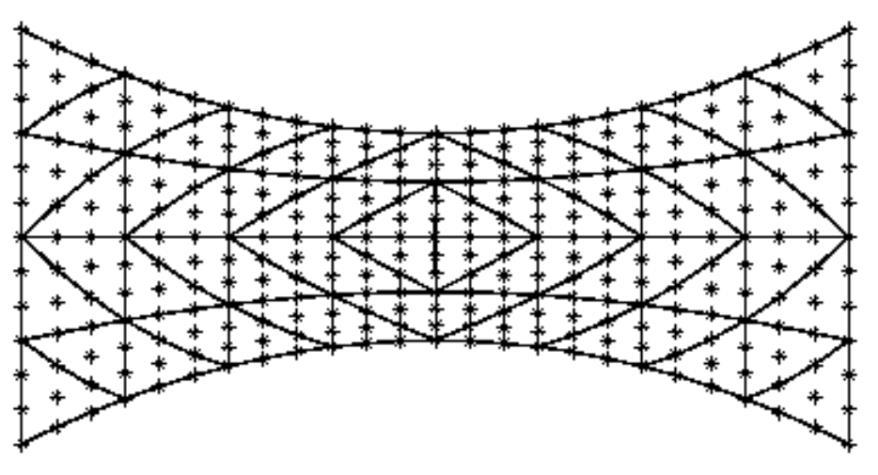
28 The natural coordinates polynomial variation for Serendipity quadrilaterals are incomplete. The polynomials for the first three members are: P(a, b) = c 1 + c 2 a +c 3 b + c 4 ab (for SQ4) + c 5 a 2 + c 6 b 2 + c 7 a 2 b + c 8 ab 2 (for SQ8) + c 9 a 3 + c 10 b 3 + c 11 a 3 b + c 12 ab 3 (for SQ12). The corresponding interpolation arrays were first published in Unfortunately the widely published interpolation functions for the SQ12 are incorrect due to a topographical error in the original article. The incorrect functions do NOT satisfy the necessary condition that they must sum to unity at any interior point, k H k (a, b) 1. The correct forms can be calculated symbolically (like the algorithm in Fig ). Due to those widespread SQ12 errors, the correct interpolations are given here. For the SQ8: For the SQ12: H 1 (a, b) = (1 2a 2b)(1 a)(1 b) H 2 (a, b) = (1 2a + 2b)(b 1)a H 3 (a, b) = ab(2a + 2b 3) H 4 (a, b) = b(a 1)(2a 2b + 1) H 5 (a, b) = (b 1)((2a 1) 2 1) H 6 (a, b) = a(1 (2b 1) 2 ) H 7 (a, b) = b(1 (2a 1) 2 ) H 8 (a, b) = (a 1)((2b 1) 2 1) (2.7-1) H 1 (a, b) = (9a 2 + 9b 2 10)(1 a)(1 b)/32 H 2 (a, b) = (9a 2 + 9b 2 10)(1 + a)(1 b)/32 H 3 (a, b) = (9a 2 + 9b 2 10)(1 + a)(1 + b)/32 H 4 (a, b) = (9a 2 + 9b 2 10)(1 a)(1 + b)/32 H 5 (a, b) = (1 3a a 2 + 3a 3 )(1 b)9/32 H 6 (a, b) = (1 3b b 2 + 3b 3 )(1 + a)9/32 H 7 (a, b) = (1 + 3a a 2 3a 3 )(1 + b)9/32 H 8 (a, b) = (1 + 3b b 2 3b 3 )(1 a)9/32 H 9 (a, b) = (1 + 3a a 2 3a 3 )(1 b)9/32 H 10 (a, b) = (1 + 3b b 2 3b 3 )(1 + a)9/32 H 11 (a, b) = (1 3a a 2 + 3a 3 )(1 + b)9/32 H 12 (a, b) = (1 3b b 2 + 3b 3 )(1 a)9/32 (2.7-2) Of course, the SQ4 interpolation is identical to the Lagrangian Q4 given in (2.5-2). The Serendipity quadrilateral elements SQ4, SQ8, and SQ12 are included in the provided element library in function Serendipity_quads.m. A mesh with the most common Serendipity quadrilaterals is shown in Fig All of the Serendipity quadrilateral elements shown there were created with the structured mesh generator presented in Appendix A. 28

29 Figure Mesh of Serendipity quadrilaterals SQ8, SQ12, SQ16, and SQ Hierarchical interpolation*: Another type of interpolation that is useful for adaptive analysis, is called hierarchical functions. The unique feature of these interpolations is that the higher order polynomials, with a new type of degree of freedom, are simply added the lower order ones. This concept is shown in one-dimension in Fig Thus, to get new functions you simply add some terms to the old functions. To illustrate this concept let us return to the linear element in local natural coordinates. In that element: u(a) = H 1 (a)u 1 e + H 2 (a)u 2 e (2.8-1) where the two H j are the linear interpolations given in (4.10). The goal is to generate a quadratic interpolation form that will not destroy the lower order functions, H j (a). The key to accomplishing that is to note that the second derivative of (2.8-1) is everywhere zero. Thus, introduce a new degree of freedom related to the second derivative of u(x) which will not affect the linear terms. Figure shows the linear element with a third control node at the midpoint (a = 0) to be associated with the quadratic additions. There the new degree of freedom be the second local derivative, d 2 u e dx 2. Upgrade the lower order approximation by adding a polynomial that is one degree higher (quadratic): u(a) = H 1 (a)u e 1 + H 2 (a)u e 2 + H 3 (a) d 2 u e dx 2. (2.8-2) This is called increasing the hierarchic of the approximation, and such elements are known as hierarchical elements. When hierarchical functions are utilized, the element matrices for a p-th order polynomial are partitions of the element matrices for a (p+1) order polynomial. 29

30 Figure Concept of hierarchical shape functions The hierarchical quadratic addition is: H 3 (a) = c 1 + c 2 a + c 3 a 2. The three constants are found from the conditions that H 3 vanishes at the two original nodes, so as not to change H 1 and H 2, and the second derivative is unity at the new midpoint node. There are various functions that satisfy those conditions, after being multiplied by a scaling constant. The element square matrix always involves an integral of the product of the derivatives of the interpolation functions. If those derivatives were orthogonal then they would result in a diagonal square matrix. That would be very desirable. It is well known that integrals of products of Legendre polynomials are orthogonal. This suggests that it would be useful to pick interpolation functions that are integrals of Legendre polynomials so that their derivatives are Legendre polynomials. The first six Legendre polynomials are P 0 (a) = 1 P 1 (a) = a P 2 (a) = (3a 2 1)/2 P 3 (a) = (5a 3 3a)/2 P 4 (a) = (35a 4 30a 2 + 3)/8 P 5 (a) = (63a 5 70a a)/8 P 6 (a) = (231a 6 315a a 2 5)/16 To avoid round off error and unnecessary calculations, there are recursion relations that should be used when computing the above Legendre polynomials. To create a family of functions for use as hierarchical interpolation functions the properties of Legendre polynomials suggest using the relation defining the sequence of functions ψ j (a) = P j (a) P j 2 (a). The first five are ψ 2 (a) = 3(a 2 1)/2 ψ 3 (a) = 5(a 3 a)/2 ψ 4 (a) = 7(5a 4 6a 2 + 1)/8 ψ 5 (a) = 9(7a 5 10a 3 + 3a)/8 ψ 6 (a) = 11(21a 6 35a a 2 1)/16 (2.8-3) 30

31 When ψ 2 is divided by 3 its second derivative is unity. Likewise, all of the ψ j functions can be scaled with a constant, λ j, to have the j-th (tangential) derivative become unity and be zero at the vertices a = ±1. Therefore, the midpoint hierarchical interpolation functions are taken as H j (a) = ψ j 1 (a)/λ j 1, j 3 (2.8-4) Figure illustrates how adding ψ 2 through ψ 4 to a two-node linear line element (or edge) can be used to enrich the element from degree p = 1 through p = 4. Figure shows that the quadratic or cubic line elements used before can also be enriched to higher degree polynomials by adding hierarchical functions beginning with one degree higher. Note that if the above domain was the edge of a two-dimensional element then the above derivatives would be viewed as tangential derivatives on that edge. The same is true for edges of solid elements. The hierarchical interpolations are most useful in adaptive programs having an error estimator. Changing just the polynomial degree in a mesh is called p-adaptivity. Changing the element sizes due to local error estimates is called h-adaptivity. Rather than change the mesh to make the element smaller in regions of high error its (and any element neighbor s) polynomial degree can be increased by one. Conversely the degree can be decreased by one rather than making the element larger in regions of low error. Of course, both changes can be made to reduce the error, and that is called hp-adaptivity. It has been shown that such an approach gives the fastest error reduction. However, it is a challenge to program that sort of adaptivity, but it is quite rewarding when accomplished. The hierarchical line (edge) element has more degrees of freedom (DOF) at a hierarchical node than at the end vertices (or other standard nodes). That slightly complicates the system equation vector subscript (herein index) that must be used to gather or scatter all of the element s DOF. That requires having the number of DOF at every node. That list, say dof_n, is easily built by first setting them all to zero. Then, as the element connections (and element type) are read the first element to connect to a node will define the number of DOF at that node. In other words, a vertex node would be set to the number of DOF for a vertex (n g ) while a hierarchical node would be set to the number of enriching hierarchical DOF (n h ), etc. One other integer array, of size (n m + 1), is required containing the sum of all of the prior DOF on the previous nodes. Denote that array with the name prior. Then the first entry is prior (1) = 0 and the last entry defines the total number of equations to be solved, prior (n m + 1) = n d, and is used to allocate memory for the system square and column matrices. In other words, the number of system dof occurring before node j is prior (j) and the number of DOF at that node is n gj = prior (j + 1) prior (j) (2.8-5) These minor changes are included in the function get_element_index_varies.m which would replace the function get_element_index.m which is used throughout this text. 31

32 Figure Creating Lagrange and hierarchical Legendre polynomials to degree 4 Figure Any Lagrangian line element can be hierarchically enriched 32

33 Example Given: A two element mesh of linear elements (L2) is each enriched with three hierarchical DOF at their mid-points. Construct the prior array to determine the total number of unknowns and the system index for each element. Solution: First sketch the mesh, the number of mesh nodes is n m = 5, the number of elements is n e = 2, the number of nodes per element is n n = 3. This application sets the number of unknowns at any standard node as n g = 1 and the number of unknowns at a hierarchical node as n h = 3. DOF Connections: [1 2 3] * * * * * [3 4 5] Node Eqs. 1 2,3,4 5 6,7,8 9 The first (1 n m ) system degree of freedom array is dof_n = [n g n h n g n h n g ] = [ ] and the second (1 (n m + 1)) DOF array is prior = [0 (0 + n g ) (n g + n h ) (n g + n h + n g ) ] = [ ] The last entry sets the size of the system rows and columns to be n d = 9. The DOF numbers for any standard node, say k, in the mesh are [(prior(k) + 1) (prior(k) + 2) (prior(k) + n g )] and at a hierarchical node n g is replaced with n h. The index of system equation numbers for an element is built up by appending that list for each of its nodes. Therefore, the first and second elements index arrays, for n i = 5 DOF per element, are: [{0 + 1} {(1 + 1) (1 + 2) (1 + 3)} {4 + 1}] = [ ] [{4 + 1} {(5 + 1) (5 + 2) (5 + 3)} {8 + 1}] = [ ]. 33

34 2.9 Summary and Notation n b Number of boundary segments n e Number of elements n g Number of generalized DOF per node n i Element independent DOF n m Number of mesh nodes n n Number of nodes per element n p Dimension of parametric space n s Dimension of physical space b = boundary segment number e = element number Element Type Element interpolation functions given in this chapter Example or Polynomial (Equation) Degree n p n g n n n i Continuity Level Lagrange L2 (2.2-6) C 0 Lagrange L3 (2.2-1) C 0 Lagrange L ,2, C 0 Hermite L2C1 (2.4-3) C 1 Hermite L3C1 (2.4-1) C 1 Hermite L2C2 Summary C 2 Lagrange T (2.6-1) C 0 Lagrange T6 (2.6-2) C 0 Lagrange Q4 (2.5-1,2) C 0 Serendipity SQ8 x (2.7-1) C 0 Serendipity SQ12 (2.7-2) C 0 Lagrange P C 0 Lagrange H8 Summary C 0 Parametric interpolations: u(r) = H(r) δ e = H k (r) δ k e k = δ et H(r) T Natural line coordinates 1 a +1: r = (a + 1) 2, a = 2r 1 Lagrange linear C 0 line interpolations (n p = 1), in unit coordinates:, H(r) = [(1 r) r], local nodes at (r = 0) and (r = 1), n n = 2, n g = 1, δ et = [u 1 u 2 ] Lagrange quadratic C 0 line interpolations (n p = 1), in unit coordinates: H(r) = [(1 3r + 2r 2 ) (4r 4r 2 ) ( r + 2r 2 )], local nodes at (r = 0), (r = 1/2) and (r = 1), n n = 3, n g = 1, δ et = [u 1 u 2 u 3 ] Lagrange cubic C 0 line interpolations (n p = 1), in unit coordinates: H(r) = 1 2 [(2 11r + 18r2 9r 3 ) (18r 45r r 3 ) ( 9r + 36r 2 27r 3 ) (2r 9r 2 + 9r 3 )], local nodes at (r = 0), (r = 1/3), (r = 2/3) and (r = 1), n n = 4, n g = 1, δ et = [u 1 u 2 u 3 u 4 ] 34

35 Lagrange linear triangle C 0 interpolation (n p = 2), in unit coordinates: H(r, s) = [(1 r s) (r) (s)], local nodes at (r = 0, s = 0), (r = 1, s = 0), and (r = 0, s = 1), n n = 3, n g = 1, δ et = [u 1 u 2 u 3 ]. Lagrange linear triangle C 0 interpolation in physical coordinates 1 H = [H 1 H 2 H 3 ]; H i (x, y) = 2A e i + b i x + c i y] 2A e = a 1 + a 2 + a 3 = b 2 c 3 b 3 c 2 : ijk a i = x j y k x k y j, b i = y j y k, c i = x k x j a 1 = x 2 y 3 x 3 y 2, a 2 = x 3 y 1 x 1 y 3, a 3 = x 1 y 2 x 2 y 1 b 1 = y 2 y 3, b 2 = y 3 y 1, b 3 = y 1 y 2 c 1 = x 3 x 2, c 2 = x 1 x 3, c 3 = x 2 x 1 Lagrange Bi-linear quadrilateral C 0 interpolation (n p = 2), in unit coordinates: H(r, s) = [(1 r s + rs) (r rs) (rs) (s rs)], local nodes at (r = 0, s = 0), (r = 1, s = 0), (r = 1, s = 1) and (r = 0, s = 1), n n = 4, n g = 1. In natural coordinates: H k (a, b) = 1 4 (1 + a a k )(1 + b b k ), a k = ±1, b k = ±1, δ et = [u 1 u 2 u 3 u 4 ]. Lagrange Tri-linear hexahedra C 0 interpolation (n p = 3), in natural coordinates: H k (a, b, c) = 1 8 (1 + a a k )(1 + b b k )(1 + c c k ), a k = ±1, b k = ±1, c k = ±1, δ et = [u 1 u 2 u 3 u 4 u 5 u 6 u 7 u 8 ]. Lagrange linear tetrahedron Lagrange interpolation (n p = 3), in unit coordinates: H(r, s, t) = [(1 r s t) (r) (s) (t)], local nodes at (r = 0, s = 0, t = 0), (r = 1, s = 0, t =0), (r = 0, s = 1, t = 0), and (r = 0, s = 0, t = 1), n n = 4, n g = 1, δ et = [u 1 u 2 u 3 u 4 ]. Hermite cubic C 1 line interpolations (n p = 1), in unit coordinates (L is physical length): H(r) = [(1 3r 2 + 2r 3 ) (r 2r 2 + r 3 )L (3r 2 2r 3 ) (r 3 r 2 )L], local nodes at (r = 0) and (r = 1), n n = 2, n g = 2, δ et = [u 1 θ 1 u 2 θ 2 ], θ = du dx. Hermite quintic C 1 line interpolations (n p = 1), in unit coordinates (L is physical length): H(r) = [(1 23r r 3 68r r 5 ) (r 6r r 3 12r 4 + 4r 5 )L (16r 2 32r r 4 ) ( 8r r 3 40r r 5 )L (7r 2 34r r 4 24r 5 ) ( r 2 + 5r 3 8r 4 + 4r 5 )L], local nodes at (r = 0), (r = 1/2) and (r = 1), n n = 3, n g = 2, δ et = [u 1 θ 1 u 2 θ 2 u 3 θ 3 ]. Hermite quintic C 2 line interpolations (n p = 1), in unit coordinates (L is physical length): H(r) = [(1 10r r 4 6r 5 ) (r 6r 3 + 8r 4 3r 5 )L (r 2 3r 3 + 3r 4 r 5 )L 2 (10r 3 15r 4 + 6r 5 ) (7r 4 3r 5 4r 3 )L ( r 3 2r 4 + r 5 )L 2 ], local nodes at 35

36 (r = 0) and (r = 1), n n = 2, n g = 3, δ et = [u 1 θ 1 κ 1 u 2 θ 2 κ 2 ], θ = du dx, κ = d 2 u dx 2. 36

37 2.10 Exercises 1. A straight line runs from point x 1 to point x 2 and has a linear line load running with a value of p 1 at the first end to point value p 2 at the other end. Their data are: Node k r k x k (m) p k (N/m) Using parametric linear interpolation, of a two-node element, find the position and value of the line load at a point 35% along the length, from the first node. 2. For the above data find the non-dimensional pressure derivative, p r at the same point. 3. A straight line runs from x 1 to midpoint x 2 to x 3 and has a line load running with a value of p 1 at the first end to point value p 2 at the mid-point to a value of p 3 at the other end. Their data are Node k r k x k (m) p k (N/m) Using parametric linear interpolation find the position, line load value, and local derivative, p r, of the line load at a point 35% along the length, from the first node. 4. A linear triangle has a normal pressure ranging from p 1 = 40 to p 2 = 46 to p 3 = 34 N m 2 at its three corners. The local nodes are at (0, 0), (1, 0), and (0, 1) respectively. Using parametric unit coordinate linear interpolation, for a T3 element, find the pressure value, and the parametric pressure gradient, p r and p s, at a non-dimensional interior point (r = 0.32, s = 0.43) Index axis, 13 beam element, 16 bi-linear quadrilateral, 38 case, 8 circular arc, 10 continuity level, 1 cubic interpolation, 5, 8, 9, 11 curvature, 1 DOF per element, 36 el_shape_n_local_deriv.m, 7, 26 element connections, 34 element neighbor, 34 error estimator, 34 Exercises, 39 for, 13 fprintf, 13 get_element_index.m, 35 gradient, 12 H8_C0, 38 h-adaptivity, 34 Hermite interpolation, 1, 16 Hermite_1D_C1_library.m, 17, 18 37

38 hierarchical interpolation, 32 hierarchical node, 32 hp-adaptivity, 34 incorrect interpolation functions, 31 inter-element continuity, 30 isoparametric, 25 Jacobian, 9 Jacobian determinant, 9 Jacobian inverse, 9 L2_C0, 6, 37 L2_C1, 37, 38 L2_C2, 37, 38 L3_C0, 6, 37 L3_C1, 16, 38 L4_C0, 8, 13, 37 Lagrange interpolation, 1, 2 Lagrange_quadrilaterals.m, 21, 24 Lagrangian_1D_library.m, 7, 8 Lagrangian_triangles.m, 26 Legendre polynomials, 33 linear interpolation, 4, 7 linear tetrahedron, 38 linear triangle, 24, 25, 39 local derivatives, 4 matrix partition, 32 measure, 7, 26 natural coordinates, 10, 15, 37 non-dimensional area, 26 orthogonality, 33 P4_C0, 26, 30, 38 p-adaptivity, 34 parabola, 11 parametric coordinates, 8 parametric derivatives, 4 physical derivative, 8 physical gradient, 8 physical length, 7, 16 plot, 13 polynomial interpolation, 1 pressure gradient, 39 print, 13 prior DOF, 34 Q16, 23 Q25, 23 Q4_C0, 20, 22, 38 Q8_C0, 20 Q9, 23 quadratic interpolation, 2, 5, 6, 7, 32 quadratic line element, 2 quadrilateral element, 20 quintic interpolation, 5, 16 real, 16 recursion relations, 33 scaling constant, 33 second derivatives, 33 Serendipity interpolation, 1 Serendipity quadrilaterals, 30 shape functions, 3 simplex element, 24 SQ12, 31 SQ16, 32 SQ17, 32 SQ8, 31, 37 standard nodes, 34 sum to unity, 4 Summary, 37 switch, 8 symbolic derivation, 16, 20, 22, 30 syms, 16 T10, 28 T15, 28 T3_C0, 24, 37 T6_C0, 26 tangential derivative, 34 tetrahedra, 24 thermal conductivity, 10 unit coordinates, 9, 24 vector subscript, 34 38