Ordinary Differential Equations I

Transcription

1 Ordinary Differential Equations I CS 205A: Mathematical Methods for Robotics, Vision, and Graphics Justin Solomon CS 205A: Mathematical Methods Ordinary Differential Equations I 1 / 32

2 Theme of Last Few Weeks The unknown is an entire function f. CS 205A: Mathematical Methods Ordinary Differential Equations I 2 / 32

3 New Twist So far: f (or its derivative/integral) known at isolated points CS 205A: Mathematical Methods Ordinary Differential Equations I 3 / 32

4 New Twist So far: f (or its derivative/integral) known at isolated points Instead: Optimize properties of f CS 205A: Mathematical Methods Ordinary Differential Equations I 3 / 32

5 Example Problems Approximate f 0 with f but make it smoother (or sharper!) CS 205A: Mathematical Methods Ordinary Differential Equations I 4 / 32

6 Example Problems Approximate f 0 with f but make it smoother (or sharper!) Simulate some dynamical or physical relationship as f(t) where t is time CS 205A: Mathematical Methods Ordinary Differential Equations I 4 / 32

7 Example Problems Approximate f 0 with f but make it smoother (or sharper!) Simulate some dynamical or physical relationship as f(t) where t is time Approximate f 0 with f but transfer properties of g 0 CS 205A: Mathematical Methods Ordinary Differential Equations I 4 / 32

8 Today: Initial Value Problems Find f(t) : R R n Satisfying F [t, f(t), f (t), f (t),..., f (k) (t)] = 0 Given f(0), f (0), f (0),..., f (k 1) (0) CS 205A: Mathematical Methods Ordinary Differential Equations I 5 / 32

9 Today: Initial Value Problems Find f(t) : R R n Satisfying F [t, f(t), f (t), f (t),..., f (k) (t)] = 0 Given f(0), f (0), f (0),..., f (k 1) (0) Example of canonical form (on board): y = ty cos y CS 205A: Mathematical Methods Ordinary Differential Equations I 5 / 32

10 Most Famous Example F = m a Newton s second law CS 205A: Mathematical Methods Ordinary Differential Equations I 6 / 32

11 Most Famous Example F = m a Newton s second law F (t, x, x ) usual expression of force CS 205A: Mathematical Methods Ordinary Differential Equations I 6 / 32

12 Most Famous Example F = m a Newton s second law F (t, x, x ) usual expression of force n particles = simulation in R 3n CS 205A: Mathematical Methods Ordinary Differential Equations I 6 / 32

13 Protein Folding CS 205A: Mathematical Methods Ordinary Differential Equations I 7 / 32

14 Gradient Descent min x E( x) CS 205A: Mathematical Methods Ordinary Differential Equations I 8 / 32

15 Gradient Descent min x E( x) = x i+1 = x i h E( x i ) CS 205A: Mathematical Methods Ordinary Differential Equations I 8 / 32

16 Gradient Descent min x E( x) = x i+1 = x i h E( x i ) = h 0 d x dt = E( x) CS 205A: Mathematical Methods Ordinary Differential Equations I 8 / 32

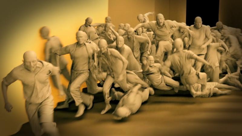
17 Crowd Simulation CS 205A: Mathematical Methods Ordinary Differential Equations I 9 / 32

18 Examples of ODEs y = 1 + cos t: solved by integrating both sides CS 205A: Mathematical Methods Ordinary Differential Equations I 10 / 32

19 Examples of ODEs y = 1 + cos t: solved by integrating both sides y = ay: linear in y, no dependence on t CS 205A: Mathematical Methods Ordinary Differential Equations I 10 / 32

20 Examples of ODEs y = 1 + cos t: solved by integrating both sides y = ay: linear in y, no dependence on t y = ay + e t : time and value-dependent CS 205A: Mathematical Methods Ordinary Differential Equations I 10 / 32

21 Examples of ODEs y = 1 + cos t: solved by integrating both sides y = ay: linear in y, no dependence on t y = ay + e t : time and value-dependent y + 3y y = t: multiple derivatives of y CS 205A: Mathematical Methods Ordinary Differential Equations I 10 / 32

22 Examples of ODEs y = 1 + cos t: solved by integrating both sides y = ay: linear in y, no dependence on t y = ay + e t : time and value-dependent y + 3y y = t: multiple derivatives of y y sin y = e ty : nonlinear in y and t CS 205A: Mathematical Methods Ordinary Differential Equations I 10 / 32

23 Reasonable Assumption Explicit ODE An ODE is explicit if can be written in the form f (k) (t) = F [t, f(t), f (t), f (t),..., f (k 1) (t)]. CS 205A: Mathematical Methods Ordinary Differential Equations I 11 / 32

24 Reasonable Assumption Explicit ODE An ODE is explicit if can be written in the form f (k) (t) = F [t, f(t), f (t), f (t),..., f (k 1) (t)]. Otherwise need to do root-finding! CS 205A: Mathematical Methods Ordinary Differential Equations I 11 / 32

25 Reduction to First Order f (k) (t) = F [t, f(t), f (t), f (t),..., f (k 1) (t)] CS 205A: Mathematical Methods Ordinary Differential Equations I 12 / 32

26 Reduction to First Order f (k) (t) = F [t, f(t), f (t), f (t),..., f (k 1) (t)] d dt f 0 (t) f 1 (t). f k 2 (t) f k 1 (t) = f 1 (t) f 2 (t). f k 1 (t) F [t, f 0 (t), f 1 (t),..., f k 1 (t)] CS 205A: Mathematical Methods Ordinary Differential Equations I 12 / 32

27 Example y = 3y 2y + y CS 205A: Mathematical Methods Ordinary Differential Equations I 13 / 32

28 Example y = 3y 2y + y d dt y z w = y z w CS 205A: Mathematical Methods Ordinary Differential Equations I 13 / 32

29 Time Dependence CS 205A: Mathematical Methods Ordinary Differential Equations I 14 / 32

30 Time Dependence Visualization: Slope field CS 205A: Mathematical Methods Ordinary Differential Equations I 14 / 32

31 Autonomous ODE y = F [ y] No dependence of F on t CS 205A: Mathematical Methods Ordinary Differential Equations I 15 / 32

32 Autonomous ODE y = F [ y] No dependence of F on t g (t) = ( f (t) ḡ (t) ) = ( F [f(t), ḡ(t)] 1 ) CS 205A: Mathematical Methods Ordinary Differential Equations I 15 / 32

33 Visualization: Phase Space θ = sin θ CS 205A: Mathematical Methods Ordinary Differential Equations I 16 / 32

34 Visualization: Traces x = σ(y x), y = x(ρ z) y, z = xy βz CS 205A: Mathematical Methods Ordinary Differential Equations I 17 / 32

35 Existence and Uniqueness dy dt = 2y t Two cases: y(0) = 0, y(0) 0 CS 205A: Mathematical Methods Ordinary Differential Equations I 18 / 32

36 Existence and Uniqueness Theorem: Local existence and uniqueness Suppose F is continuous and Lipschitz, that is, F [ y] F [ x] 2 L y x 2 for some fixed L 0. Then, the ODE f (t) = F [f(t)] admits exactly one solution for all t 0 regardless of initial conditions. CS 205A: Mathematical Methods Ordinary Differential Equations I 19 / 32

37 Linearization of 1D ODEs y = F [y] CS 205A: Mathematical Methods Ordinary Differential Equations I 20 / 32

38 Linearization of 1D ODEs y = F [y] y = ay + b CS 205A: Mathematical Methods Ordinary Differential Equations I 20 / 32

39 Linearization of 1D ODEs y = F [y] y = ay + b ȳ = aȳ CS 205A: Mathematical Methods Ordinary Differential Equations I 20 / 32

40 Model Equation y = ay CS 205A: Mathematical Methods Ordinary Differential Equations I 21 / 32

41 Model Equation y = ay = y(t) = Ce at CS 205A: Mathematical Methods Ordinary Differential Equations I 21 / 32

42 Stability: Visualization y = ay CS 205A: Mathematical Methods Ordinary Differential Equations I 22 / 32

43 Three Cases y = ay, y(t) = Ce at 1. a = 0: Stable CS 205A: Mathematical Methods Ordinary Differential Equations I 23 / 32

44 Three Cases y = ay, y(t) = Ce at 1. a = 0: Stable 2. a < 0: Stable; solutions get closer CS 205A: Mathematical Methods Ordinary Differential Equations I 23 / 32

45 Three Cases y = ay, y(t) = Ce at 1. a = 0: Stable 2. a < 0: Stable; solutions get closer 3. a > 0: Unstable; mistakes in initial data amplified CS 205A: Mathematical Methods Ordinary Differential Equations I 23 / 32

46 Intuition for Stability An unstable ODE magnifies mistakes in the initial conditions y(0). CS 205A: Mathematical Methods Ordinary Differential Equations I 24 / 32

47 Multidimensional Case y = A y, A y i = λ i y i y(0) = i c i y i CS 205A: Mathematical Methods Ordinary Differential Equations I 25 / 32

48 Multidimensional Case y = A y, A y i = λ i y i y(0) = i c i y i = y(t) = i c i e λ it y i CS 205A: Mathematical Methods Ordinary Differential Equations I 25 / 32

49 Multidimensional Case y = A y, A y i = λ i y i y(0) = i c i y i = y(t) = i c i e λ it y i Stability depends on max i λ i. CS 205A: Mathematical Methods Ordinary Differential Equations I 25 / 32

50 Integration Strategies Given y k at time t k, generate y k+1 assuming y = F [ y]. CS 205A: Mathematical Methods Ordinary Differential Equations I 26 / 32

51 Forward Euler y k+1 = y k + hf [ y k ] Explicit method O(h 2 ) localized truncation error O(h) global truncation error; first order accurate CS 205A: Mathematical Methods Ordinary Differential Equations I 27 / 32

52 Forward Euler: Stability CS 205A: Mathematical Methods Ordinary Differential Equations I 28 / 32

53 Model Equation y = ay y k+1 = (1 + ah)y k For a < 0, stable when h < 2 a. CS 205A: Mathematical Methods Ordinary Differential Equations I 29 / 32

54 Backward Euler y k+1 = y k + hf [ y k+1 ] Implicit method O(h 2 ) localized truncation error O(h) global truncation error; first order accurate CS 205A: Mathematical Methods Ordinary Differential Equations I 30 / 32

55 Forward Euler: Stability CS 205A: Mathematical Methods Ordinary Differential Equations I 31 / 32

56 Model Equation y = ay y k+1 = 1 1 ah y k Unconditionally stable! CS 205A: Mathematical Methods Ordinary Differential Equations I 32 / 32

57 Model Equation y = ay y k+1 = 1 1 ah y k Unconditionally stable! But this has nothing to do with accuracy. CS 205A: Mathematical Methods Ordinary Differential Equations I 32 / 32

58 Model Equation y = ay y k+1 = 1 1 ah y k Unconditionally stable! But this has nothing to do with accuracy. Good for stiff equations. CS 205A: Mathematical Methods Ordinary Differential Equations I 32 / 32

59 Forward and Backward Euler on Linear ODE y = A y Forward Euler: y k+1 = (I + ha) y k Backward Euler: y k+1 = (I ha) 1 y k Next CS 205A: Mathematical Methods Ordinary Differential Equations I 33 / 32