Chap. 20: Initial-Value Problems

Transcription

1 Chap. 20: Initial-Value Problems

2 Ordinary Differential Equations Goal: to solve differential equations of the form: dy dt f t, y The methods in this chapter are all one-step methods and have the general format: where is called an increment function, and is used to extrapolate from an old value y i to a new value y i+1. y i1 y i h 2

3 Euler s Method The first derivative provides a direct estimate of the slope at t i : dy dt ti f t i, y i and the Euler method uses that estimate as the increment function: f t i, y i y i1 y i f t i, y i h 3

4 Example 20.1 Solve y =4e 0.8t -0.5y with y(0)=2. Analytical solution: y=4/1.3 (e 0.8t -e -0.5t )+2e -0.5t 4

5 Error Analysis for Euler s Method The numerical solution of ODEs involves two types of error: Truncation errors, caused by the nature of the techniques employed Roundoff errors, caused by the limited numbers of significant digits that can be retained The total, or global truncation error can be further split into: local truncation error that results from an application method in question over a single step, and propagated truncation error that results from the approximations produced during previous steps. 5

6 Error Analysis for Euler s Method The local truncation error for Euler s method is O(h 2 ) and proportional to the derivative of f(t,y) while the global truncation error is O(h). This means: The global error can be reduced by decreasing the step size, and Euler s method will provide error-free predictions if the underlying function is linear. Euler s method is conditionally stable, depending on the size of h. 6

7 Example dy dt ay Analytical Solution: yy 0 e at Euler s method: y i1 y i ay i hy i (1ah) 1-ah is called an amplification factor. Convergence condition: 1-ah <1 7

8 Heun s Method One method to improve Euler s method is to determine derivatives at the beginning and predicted ending of the interval and average them: 8

9 Heun s Method (cont.) This process relies on making a prediction of the new value of y, then correcting it based on the slope calculated at that new value. This predictor-corrector approach can be iterated to convergence: 9

10 Example 20.2 Solve y =4e0.8t-0.5y with y(0)=2. Stopping criterion: %. Analytical solution: y=4/1.3 (e0.8t-e-0.5t)+2e-0.5t 10

11 Midpoint Method Another improvement to Euler s method is similar to Heun s method, but predicts the slope at the midpoint of an interval rather than at the end: This method has a local truncation error of O(h 3 ) and global error of O(h 2 ) 11

12 Runge-Kutta Methods Runge-Kutta (RK) methods achieve the accuracy of a Taylor series approach without requiring the calculation of higher derivatives. For RK methods, the increment function can be generally written as: a 1 k 1 a 2 k 2 a n k n where the a s are constants and the k s are k 1 f t i, y i k 2 f t i p 1 h, y i q 11 k 1 h k 3 f t i p 2 h, y i q 21 k 1 h q 22 k 2 h k n ft i p n1 h, y i q n1,1 k 1 h q n1,2 k 2 h q n1,n1 k n1 h where the p s and q s are constants. 12

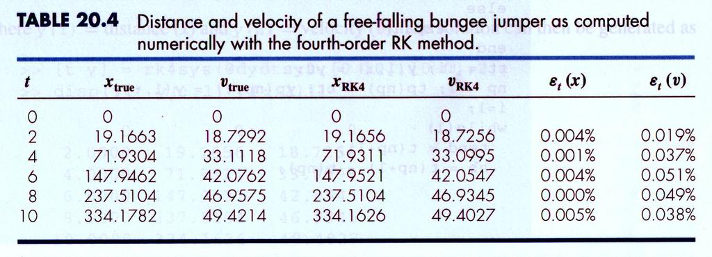
13 Classical Fourth-Order Runge-Kutta Method The most popular RK methods are fourthorder, and the most commonly used form is: y i1 y i 1 6 k 1 2k 2 2k 3 k 4 h where: k 1 f t i, y i k 2 f t i 1 2 h, y i 1 2 k 1h k 3 f t i 1 2 h, y 1 i 2 k h 2 k 4 f t i h, y i k 3 h 13

14 Example 20.3 Use Classical Fourth-Order RK Method to solve Example t true RK4 Error(%)

15 Systems of Equations Many practical problems require the solution of a system of equations: dy 1 dt f 1 t, y, y,, y 1 2 n dy 2 f 2 t, y 1, y 2,, y n dt dy n f n t, y 1, y 2,, y n dt The solution of such a system requires that n initial conditions be known at the starting value of t. 15

16 Solution Methods Single-equation methods can be used to solve systems of ODE s as well; for example, Euler s method can be used on systems of equations - the one-step method is applied for every equation at each step before proceeding to the next step. Fourth-order Runge-Kutta methods can also be used, but care must be taken in calculating the k s. 16

17 Example 20.5 Solve dx dt v dv dt g c d m v 2 function dy=dydtsys(t,y) dy=[y(2); /68.1*y(2)^2]; [t y]=rk4sys(dydtsys,[0 10],[0,0],2); Initial condition: x(0)=0, v(0)=0 Analytical solution: v(t) gm tanh c d gc d m t x(t) m ln cosh c d gc d m t 17

18 Example (cont.) 18

19 Case Study: Predator-Prey Models and Chaos Predator-Prey Models dx dt axbxy dy dt cydxy x: the number of prey y: the number of predator a: prey growth rate c: predator death rate b: prey death rate due to predator d: predator growth rate due to prey 19

20 Example Let a=1.2, b=0.6, c=0.8 and d=0.3. Initial condition: x=2, y=1. t=0 to 30, h=

21 Lorenz Equations dx dt σxσy dy dt rxyxz dz dt bzxy Chaotic behavior. Bounded but not periodic. Sensitive to initial value. 21

22 Strange Attractors 22

23 Strange Attractors (cont.) 23