A Hierarchy of Support Vector Machines for Pattern Detection
|
|
|
- Maurice Watkins
- 6 years ago
- Views:
Transcription
1 A Hierarchy of Support Vector Machines for Pattern Detection Hichem Sahbi Imedia research Group INRIA Rocquencourt, BP Le Chesnay cedex, FRANCE Donald Geman Center for Imaging Science 302 Clark Hall Johns Hopkins University 3400 N. Charles Street Baltimore, MD Editor: Pietro Perona Abstract We introduce a computational design for pattern detection based on a treestructured network of support vector machines (SVMs). An SVM is associated with each cell in a recursive partitioning of the space of patterns (hypotheses) into increasingly finer subsets. The hierarchy is traversed coarse-to-fine and each chain of positive responses from the root to a leaf constitutes a detection. Our objective is to design and build a network which balances overall error and computation. Initially, SVMs are constructed for each cell with no constraints. This free network is then perturbed, cell by cell, into another network, which is graded in two ways: first, the number of support vectors of each SVM is reduced (by clustering) in order to adjust to a pre-determined, increasing function of cell depth; second, the decision boundaries are shifted to preserve all positive responses from the original set of training data. The limits on the numbers of clusters (virtual support vectors) result from minimizing the mean computational cost of collecting all detections subject to a bound on the expected number of false positives. When applied to detecting faces in cluttered scenes, the patterns correspond to poses and the free network is already faster and more accurate than applying a single pose-specific SVM many times. The graded network promotes very rapid processing of background regions while maintaining the discriminatory power of the free network. Keywords: Statistical learning, hierarchy of classifiers, coarse-to-fine computation, support vector machines, face detection. c 2005 Hichem Sahbi and Donald Geman.
2 1. Introduction Our objective is to design and build a pattern detection system based on a treestructured network of increasingly complex support vector machines (SVMs) [1, 2]. The methodology is general, and could be applied to any classification task in machine learning in which there are natural groupings among the patterns (classes, hypotheses). The application which motivates this work is to detect and localize all occurrences in a scene of some particular object category based on a single, greylevel image. The particular example of detecting faces against cluttered backgrounds provides a running illustration of the ideas where the groupings are based on pose continuity. Our optimization framework is motivated by natural trade-offs among invariance, power (background rejection rate) and the cost of processing the data in order to determine all detected patterns. In particular, it is motivated by the amount of computation involved when a single SVM, dedicated to a reference pattern (e.g., faces with a nearly fixed position, scale and tilt), is applied to many data transformations (e.g., translations, scalings and rotations). This is illustrated for face detection in Fig 1; a graded network of SVMs achieves approximately the same accuracy as a pattern-specific SVM but with order 100 to 1000 times fewer kernel evaluations, resulting from the network architecture as well as the reduced number of support vectors. To design and construct such a graded network, we begin with a hierarchical representation of the space of patterns (e.g., poses of a face) in the form of a sequence of nested partitions, one for each level in a binary tree [3, 4, 5, 6, 7, 8, 9]. Each cell - distinguished subset of patterns - encodes a simpler, sub-classification task and is assigned a binary classifier. The leaf cells represent the resolution at which we desire to detect the true pattern(s). There is also a background class, e.g., a complex and heterogeneous set of non-distinguished patterns, which is statistically dominant (i.e., usually true). A pattern is detected if the classifier for every cell which covers it responds positively. Initially, SVMs are constructed for each cell in the standard way [1] based on a kernel and training data positive examples (from a given cell) and negative examples ( background ). This is the free network, or f-network {f t }, where t denotes a node in the tree hierarchy. The graded network, or g-network {g t }, is indexed by the same hierarchy, but the number of intervening terms in each g t is fixed in advance (by clustering those in f t as in [10]), and grows with the level of t. (From here on, the vectors appearing g t will be referred to as support vectors even though, technically, they are constructed from the actual support vectors appearing in f t.) Moreover, the decision boundaries are shifted to preserve all positive responses from the original set of training data; consequently, the false negative (missed detection) rate of g t is at most that of f t and any pattern detected by the f-network is also detected by the g-network. But the g-network will be far more efficient. 2

3 Figure 1: Comparison between a single SVM (top row) dedicated to a nearly fixed pose and our designed network (bottom row) which investigates many poses simultaneously. The sizes of the three images are, left to right, , and pixels. The network achieves approximately the same accuracy as the posespecific SVM but with order times fewer kernel evaluations. Some statistics comparing efficiency are given in Table 1. 3
4 Table 1: Comparisons among i) a single SVM dedicated to a small set of hypotheses (in this case a constrained pose domain), ii) the f-network and iii) our designed g- network, for the images in Fig 1. For the single SVM, the position of the face is restricted to a 2 2 window, its scale to the range [10,12] pixels and its orientation to [ 5 0,+5 0 ]; the original image is downscaled 14 times by a factor of 0.83 and for each scale the SVM is applied to the image data around each non-overlapping 2 2 block. In the case of the f and g-networks, we use the coarse-to-fine hierarchy and the search strategy presented here. Figures Mona Lisa Singers Star Trek 1 SVM f-net g-net 1 SVM f-net g-net 1 SVM f-net g-net # Subimages Processed # Kernel Evaluations Processing Time (s) # Raw Detections The limits on the numbers of support vectors result from solving a constrained optimization problem. We minimize the mean computation necessary to collect all detections subject to a constraint on the rate of false detections. (In the application to face detection, a false detection refers to finding a face amidst clutter.) Mean computation is driven by the background distribution. This also involves a model for how the background rejection rate of an SVM depends on complexity, which is assumed proportional to the number of support vectors, and invariance, referring to the scope of the underlying cell in the hierarchy. In the free network, the complexity of each SVM decision function depends in the usual way on the underlying probability distribution of the training data. For instance, the decision function for a linearly separable training set might be expressed with only two support vectors, whereas the SVMs induced from complex tasks in object recognition usually involve many support vectors [2]. For the f-network, the complexity generally decreases as a function of depth due to the progressive simplification of the underlying tasks. This is illustrated in Fig 2 (left) for face detection; the classifiers f t were each trained on 8000 positive examples and 50, 000 negative examples. Put differently, complexity increases with invariance. Consider an SVM f in the f-network with N support vectors and dedicated to a particular hypothesis cell; this network is slow, but has high power and few false negatives. The corresponding SVM g has a specified number n of support vectors with n N. It is intuitively apparent that the power of g is smaller; this is the price for maintaining the false negative rate and reducing the number of kernel evaluations. In particular, if n is very small, g will have low power (cf. Fig 2 (right)). In general, of course, with no constraints, the fraction of support vectors provides a rough measure of the difficulty of the problem; here, however, we are artificially reducing the number of support vectors, thereby limiting the power of the classifiers in the g-network. 4
5 Coarse classifier Fine classifier Number of support vectors False alarm rate Level 1 Level 2 Level 3 Level 4 Level 5 Level Cardinality of the reduced set Figure 2: Left: The average number of support vectors for each level in an f-network built for face detection. The number of support vectors is decreasing due to progressive simplification of the original problem. Right: False alarm rate as a function of the number of support vectors using two SVM classifiers in the g-network with different pose constraints. Building expensive classifiers at the upper levels (n N) leads to intensive early processing, even when classifying simple background patterns (e.g., flat areas in images), so the overall mean cost is also very large (cf. Fig 3, top rows). As an alternative to building the g-network, suppose we simply replace the SVMs in the upper levels of f-network with very simple classifiers (e.g., linear SVMs); then many background patterns will reach the lower levels, resulting in an overall loss of efficiency (cf. Fig 3, middle rows). We focus in between these extremes and build {g t } to achieve a certain trade-off between cost and power (cf. Fig 3, bottom rows). Of course, we cannot explore all possible designs so a model-based approach is necessary: The false alarm rate of each SVM is assumed to vary with complexity and invariance in a certain way. This functional dependence is consistent with the one proposed in [7], where the computational cost of a classifier is modeled as the product of an increasing function of scope and an increasing function of power. Finally, from the perspective of computer vision, especially image interpretation, the interest of this paper is the proposed architecture for aggregating binary classfiers such as SVMs for organized scene parsing. For some problems, dedicating a single classifier to each hypothesis, or a cascade (linear chain) of classifiers to a small subset of hypotheses (see Section 2), and then training with existing methodology (even offthe-shelf software) might suffice, in fact provide state-of-the-art performance. This seems to the case for example with frontal face detection as long as large training sets are available, at least thousands of faces and sometimes billions of negative examples, for learning long, powerful cascades. However, those approaches are either very costly (see above) or may not scale to more ambitious problems involving limited data, or 5
 # Samples 936 755 67 2 0 0 (heuristic) # Samples 1402 340 18 0 0 0 (g-network) Figure 3: In order to illustrate varying trade-offs")
6 Maximum Level Reached # Samples (f-network) # Samples (heuristic) # Samples (g-network) # Kernel Evaluations # Samples (f-network) # Samples (heuristic) # Samples (g-network) Figure 3: In order to illustrate varying trade-offs among cost, power and invariance, and to demonstrate the utility of a principled, global analysis, we classified 1760 subimages of size extracted from the image shown above using three different types of SVM hierarchies of depth six. In each case, the hierarchy was traversed coarse-to-fine. For each hierarchy type and each subimage, the upper table shows the distribution of the deepest level visited and the lower table shows the distribution of cost in terms of the total number of kernel evaluations. In both tables: Top row: The unconstrained SVM hierarchy ( f-network ) with a Gaussian kernel at all levels; the SVMs near the top are very expensive (about 1400 support vectors at the root; see Fig 2) resulting in high overall cost. Middle row: An ad hoc solution: the same f-network, except with linear SVMs (which can be assumed to have only two support vectors) at the upper three levels in order to reduce computation; many images reach deep levels. Bottom row: The constrained SVM hierarchy ( g-network ), globally designed to balance error and computation; the number of (virtual) support vectors grows with depth. 6
7 more complex and varied interpretations, because they rely too heavily on brute-force learning and lack the structure necessary to hardwire efficiency by simultaneously exploring multiple hypotheses. We believe that hierarchies of classifiers provide such a structure. In the case of SVMs, which may require extensive computation, we demonstrate that building such a hierarchy with a global design which accounts for both cost and error is superior to either a single classifier applied a great many times (a form of template-matching) or a hierarchy of classifiers constructed independently, node-by-node, without regard to overall performance. We suspect that the same demonstration could be carried out with other base classifiers as long as there is a natural method for adjusting the amount of computation; in fact, the global optimization framework could be applied to improve other parsing strategies, such as cascades. The remaining sections are organized as follows: A review of coarse-to-fine object detection, including related work on cascades, is presented in 2. In 3, we discuss hierarchical representation and search in general terms; decomposing the pose space provides a running example of the ideas and sets the stage for our main application - face detection. The f-network and g-network are defined in 4, again in general terms and the statistical framework and optimization problem are laid out in 5. This is followed in 6 by a new formulation of the reduced set method [11, 10], which is used to construct an SVM of specified complexity. These ideas are illustrated for a pose hierarchy in 7, including a specific instance of the model for chain probabilities and the corresponding minimization of cost subject to a constraint on false alarms. Experiments are provided in 8, where the g-network is applied to detect faces in standard test data, allowing us to compare our results with other methods. Finally, some conclusions are drawn in Coarse-to-Fine Object Detection Our work is motivated by difficulties encountered in inducing semantic descriptions of natural scenes from image data. This is often computationally intensive due to the large amount of data to be processed with high precision. Object detection is such an example and has been widely investigated in computer vision; see for instance [2, 3, 12, 13, 14, 15] for work on face detection. Nonetheless, there is as yet no system which matches human accuracy; moreover, the precision which is achieved often comes at the expense of run-time performance or a reliance on massive training sets. One approach to computational efficiency is coarse-to-fine processing, which has been applied to many problems in computer vision, including object detection [3, 15, 16, 17, 18, 19, 20], matching [21, 22, 23], optical flow [24], tracking [25] and other tasks such as compression, registration, noise reduction and estimating motion and binocular disparity. In the case of object detection, one strategy is to focus rapidly on areas of interest by finding characteristics which are common to many 7
.")
8 Figure 4: Left: Detections using our system. Right: The darkness of a pixel is proportional to the amount of local processing necessary to collect all detections. instantiations; in particular, background regions are quickly rejected as candidates for further processing (see Fig 4). In the context of finding faces in cluttered scenes, Fleuret and Geman [3] developed a fast, coarse-to-fine detector based on simple edge configurations and a hierarchical decomposition of the space of poses (location, scale and tilt). (Similar, tree-structured recognition strategies appear in [16, 17].) In [3], one constructs a family of classifiers, one for each cell in a recursive partitioning of the pose space and trained on a subpopulation of faces meeting the pose constraints. A face is declared with pose in a leaf cell if all the classifiers along the chain from root to leaf respond positively. In general, simple and uniform structures in the scene are quickly rejected as face locations (i.e., very few classifiers are executed before all possible complete chains are eliminated) whereas more complex regions, for instance textured areas and face-like structures, require deeper penetration into the hierarchy. Consequently, the overall cost to process a scene is dramatically lower than looping over many individual poses, a form of template- matching (cf. Fig 1). Work on cascades [15, 26, 27, 28, 29, 30, 31, 32] is also motivated by an early rejection principle to exploit skewed priors (i.e., background domination). In that work, as in ours, the time required to classify a pattern (e.g., an input subimage) depends on the resemblance between that pattern and the objects of interest. For example, Viola and Jones [15] developed an accurate, real-time face detection algorithm in the form of a cascade of boosted classifiers and computationally efficient feature detec- 8
9 tion. Other variations, such as those in [32, 30] for face detection, and the cascade of inner products in [28] for object identification, employ very simple linear classifiers. In nearly all cases the individual node learning problems are treated heuristically; an exception is [32], where, for each node, the classifiers are designed to solve a (local) optimization problem constrained by desired (local) error rates. There are several important differences between our work and cascades. Cascades are coarse-to-fine in the sense of background filtering whereas our approach is coarse-to-fine both in the sense of hierarchical pruning of the background class and representation of the space of hypotheses. In particular, cascades operate in a more or less brute-force fashion because every pose (e.g., position, scale and tilt) must be examined separately. In comparing the two strategies, especially our work with cascades of SVMs for face detection as in [31, 30], there is then a trade-off between very fast early rejection of individual hypotheses (cascades) and somewhat slower rejection of collections of hypotheses (tree-structured pruning). No systematic comparison with cascades has been attempted. Moving beyond an empirical study would require a model for how cost scales with other factors, such as scope and power. One such model was proposed in [7], in which the computational cost C(f) of a binary classifier f dedicated to a set A of hypotheses (against a universal background alternative) is expressed as C(f) = Γ( A ) Ψ(1 δ) where δ is false positive rate of the classifier f (the probability the answer is positive under the background hypothesis) and Γ and Ψ are increasing functions with Γ subadditive and Ψ convex. (Some empirical justification for this model can be found in [7].) One can then compare the cost of testing a small set A of hypotheses (e.g., all poses over a small range of locations, scales and tilts, as in cascades) versus a large set B A (e.g., many poses simultaneously, as here). Under this cost model, and equalizing the power, the subadditivity of Γ would render the test dedicated to B cheaper than doing the test dedicated to A approximately A times, even ignoring B the inevitable reduction in power due to repeated tests. More importantly, perhaps, it is not clear that cascades will scale to more ambitious problems involving many classes and instantiations since repeatedly testing a coarse set of hypotheses will lack selectivity and repeatedly testing a narrow one will require a great many implementations. Finally, to our knowledge, the work presented in this paper is the first to consider a global construction of the system in an optimization framework. In particular, no global criteria appear in either [3] or [15]; in the former, the edge-based classifiers are of roughly constant complexity whereas in the latter the complexity of the classifiers along the cascade is not explicitly controlled. 9
10 3. Hierarchical Representation and Search 3.1 Pattern Decomposition Let Λ denote a set of patterns or hypotheses of interest. Our objective is to determine which, if any, of the hypotheses λ Λ is true, the alternative being a statistically dominant background hypothesis {0}, meaning that most of the time 0 is the true explanation. Let Y denote the true state; Y = 0 denotes the background state. Instead of searching separately for each λ Λ, consider a coarse-to-fine search strategy in which we first try to exploit common properties ( shared features ) of all hypotheses to test simultaneously for all λ Λ, i.e., test the compound hypothesis H : Y Λ against the alternative H 0 : Y = 0. If the test is negative, we stop and declare background; if the test is positive, we separately test two disjoint subsets of Λ against H 0 ; and so forth in a nested fashion. The tests are constructed to be very conservative in the sense that each false negative error rate is very small, i.e., given that Y A, we are very unlikely to declare background if A Λ is the subset of hypotheses tested at a given stage. The price for this small false negative error is of course a non-negligible false positive error, particularly for testing large subsets A. However, this procedure is highly efficient, particularly under the background hypothesis. This divide-and-conquer search strategy has been extensively examined, both algorithmically (e.g.,[3, 8, 9] and mathematically ([7, 4, 6]). Note: There is an alternate formulation in which Y is directly modeled as a subset of Λ with Y = corresponding to the background state. In this case, at each node of the hierarchy, we are testing a hypothesis of the form H : Y A vs the alternative Y A =. In practice, the two formulations are essentially equivalent; for instance, in face detection, we can either decompose a set of reference poses which can represent at most one face and then execute the hierarchical search over subimages or collect all poses into one hierarchy with virtual tests near the root; see 7.1. We shall adopt the simpler formulation in which Y Λ {0}. Of course in practice we do all the splitting and construct all the tests in advance. (It should be emphasized that we are not constructing a decision tree; in particular, we are recursively partitioning the space of interpretations not features and, when the hierarchy is processed, a data point can travel down many branches and arrive at none of the leaves.) Then, on line, we need only execute the tests in the resulting hierarchy coarse-to-fine. Moreover, the tests are simply standard classifiers induced from training data - examples of Y A for various subsets of A and examples of Y = 0. In particular, in the case of object detection, the classifiers are constructed from the usual types of image features, such as averages, edges and wavelets [5]. The nested partitions are naturally identified with a tree T. There is a subset Λ t for each node t of T, including the root (Λ root = Λ) and each leaf t T. We will 10
11 write t = (l, k) to denote the k th node of T at depth or level l. For example, in the case of a binary tree T with L levels, we then have: Λ 1,1 = Λ Λ l,k = Λ l+1,2k 1 Λ l+1,2k Λ l+1,2k 1 Λ l+1,2k = l {1,..., L 1}, k { 1,..., 2 l 1} The hierarchy can be manually constructed (as here, copying the one from [3]) or, ideally, learned. Notice that the leaf cells Λ t, t T, needn t correspond to individual hypotheses. Instead, they represent the finest resolution at which we wish to estimate Y. More careful disambiguation among candidate hypotheses may require more intense processing, perhaps involving online optimization. It then makes sense to modify our definition of Y to reflect this possible coarsening of the original classification problem: the possible class values are then {0, 1,..., 2 L 1 }, corresponding to background ({0}) and the 2 L 1 fine cells at the leaves of the hierarchy. Example: The Hierarchy for Face Detection. Here, the pose of an object refers to parameters characterizing its geometric appearance in the image. Since we are searching for instances of a one object class faces the family of hypotheses of interest is a set of poses Λ. Specifically, we focus attention on the position, tilt and scale of a face, denoted θ = (p, φ, s), where p is the midpoint between the eyes, s is the distance between the eyes and φ is the angle with the line orthogonal to the segment joining the eyes. We then define Λ = { (p, φ, s) R 4 : p [ 8, +8] 2, φ [ 20 0, ], s [10, 20] } Thus, we regard Λ as a reference set of poses in the sense of possible instantiations of a single face within a given image assuming that the position is restricted to a subwindow (e.g., an centered in the subimage) and the scale to the stated range. The background hypothesis is no face (with pose in Λ). The leaves of T do not correspond to individual poses θ Λ; for instance, the final resolution on position is a 2 2 window. Hence, each object hypothesis is a small collection of fine poses. The specific hierarchy used in our experiments is illustrated in Fig (5). It has six levels (L = 6), corresponding to three quaternary splits in location (four 8 8 blocks, etc.) and one binary split both on tilt and scale. Therefore, writing ν l for the number of cells in T at depth l: ν 1 = 1, ν 2 = 4 1, ν 3 = 4 2 = 16, ν 4 = 4 3 = 64, ν 5 = = 128 and ν 6 = = 256. This is the same, manually-designed, pose hierarchy that was used in [3]. The partitioning based on individual components, as well as the splitting order, is entirely ad hoc. The important issue of how to automatically design or learn the divide-andconquer architecture is not considered here. Very recent work on this topic appears in [33] and [9]. 11
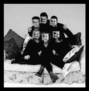
![{(p, φ, s) R 4 : p [ 8, +8] 2, φ [ 20 0, +20 0 ], s [10, 20]} {(p, φ, s) R 4 : p [ 1, +1] 2, φ [0 0, +20 0 ], s [15, 20]} Figure 5: An illustration of the pose hierarchy showing a sample of faces at](/docs-images/76/73881916/images/12-0.jpg "the root cell and at one of the leaves. 3.2 Search Strategy Consider coarse-to-fine search in more detail.")
 and X t : Ω {0, 1}.")
12 {(p, φ, s) R 4 : p [ 8, +8] 2, φ [ 20 0, ], s [10, 20]} {(p, φ, s) R 4 : p [ 1, +1] 2, φ [0 0, ], s [15, 20]} Figure 5: An illustration of the pose hierarchy showing a sample of faces at the root cell and at one of the leaves. 3.2 Search Strategy Consider coarse-to-fine search in more detail. Let X t be the test or classifier associated with node t, with X t = 1 signaling the acceptance of H t : Y Λ t and X t = 0 signaling the acceptance of H 0 : Y = 0. Also, let ω Ω represent the underlying data or pattern upon which the tests are based; hence the true class of ω is Y (ω) and X t : Ω {0, 1}. The result of coarse-to-fine search applied to ω is a subset D(ω) Λ of detections, possibly empty, defined to be all λ Λ for which X t (ω) = 1 for every test which covers λ, i.e., for which λ Λ t. Equivalently, D is the union over all Λ t, t T such that X t = 1 and the test corresponding to every ancestor of t T is positive, i.e., all complete chains of ones (cf. Fig 6, B). Both breadth-first and depth-first coarse-to-fine search lead to the same set D. Breadth-first search is illustrated in Fig (6, C): Perform X 1,1 ; if X 1,1 = 0, stop and declare D = ; if X 1,1 = 1, perform both X 2,1 and X 2,2 and stop only if both are negative; etc. Depth-first search explores the sub-hierarchy rooted at a node t before exploring the brother of t. In other words, if X t = 1, we visit recursively the subhierarchies rooted at t; if X t = 0 we cancel all the tests in this sub-hierarchy. In both cases, a test is performed if and only if all its ancestors are performed and are positive. (These strategies are not the same if our objective is only to determine whether or not D = ; see the analysis in [6].) 12
13 Notice that D = if and only if there is a null covering of the hierarchy in the sense of a collection of negative responses whose corresponding cells cover all hypotheses in Λ. The search is terminated upon finding such a null covering. Thus, for example, if X 1,1 = 0, the search is terminated as there cannot be a complete chain of ones; similarly, if X 2,1 = 0 and X 3,3 = X 3,4 = 0, the search is terminated. θ 3 θ 4 (A) (B) (C) Figure 6: A hierarchy with fifteen tests. (A) The response to an input image were all the tests to be performed; the positive tests are shown in black and negative tests in white. (B) There are two complete chains of ones; in the case of object detection, the detected pose is the average over those in the two corresponding leaves. (C) The breadth-first search strategy with the executed tests are shown in color; notice that only seven of the tests would actually be performed. Example: The Search Strategy for Face Detection. Images ω are encoded using a vector of wavelet coefficients; in the remainder of this paper we will write x to denote this vector of coefficients computed on a given subimage. If D(x), the estimated pose of the face detected in ω is obtained by averaging over the pose prototypes of each leaf cell represented in D, where the pose prototype of Λ t is the midpoint (cf. Fig 6, B). A scene is processed by visiting non-overlapping blocks, processing the surrounding image data to extract the features (wavelet coefficients) and classifying these features using the search strategy described in 3.2. This process makes it possible to detect all faces whose scale s lies in the interval [10, 20] and whose tilt belongs to [ 20 o, +20 o ]. Faces at scales [20, 160] are detected by repeated downsampling (by a factor of 2) of the original image, once for scales [20, 40], twice for [40, 80] and thrice for [80, 160](cf. Fig 7). Hence, due to high invariance to scale in the base detector, only four scales need to be investigated altogether. Alternatively, we can think of an extended hierarchy over all possible poses, with initial branching into disjoint blocks and disjoint scale ranges, and with virtual tests in the first two layers which are passed by all inputs. Given color or motion information [34], it might be possible to design a test which handles a set of poses 13
14 Figure 7: Multi-scale search. The original image (on the left) is downscaled three times. For each scale, the base face detector visits each non-overlapping block, and searches the surrounding image data for all faces with position in the block, scale anywhere in the range [10, 20] and in-plane orientation in the range [ 20 o, +20 o ]. larger than Λ; however, our test at the root (accounting simultaneously for all poses in Λ) is already quite coarse. 4. Two SVM Hierarchies Suppose we have a training set T = {(ω 1, y 1 ),..., (ω n, y n )}. In the case of object detection, each ω is some subimage taken, for example, from the Web, and either belongs to the object examples L (subimages ω for which Y (ω) 0) or background examples B (subimages for which Y (ω) = 0). All tests X t, t T, are based on SVMs. We build one hierarchy, the free network or f-network for short, with no constraints, i.e., in the usual way from the training data once a kernel and any other parameters are specified [1]. The other hierarchy, the graded network or g-network, is designed to meet certain error and complexity specifications. 14
15 4.1 The f-network Let f t be an SVM dedicated to separating examples of Y Λ t from examples of Y = 0. (In our application to face detection, we train f t based on face images ω with pose in Λ t.) The corresponding test is simply 1 {ft>0}. We refer to {f t, t T } as the f-network. In practice, the number of support vectors decreases with the depth in the hierarchy since the classification tasks are increasingly simplified; see Fig 2, left. We assume the false negative rate of f t is very small for each t; in other words, f t (ω) > 0 for nearly all patterns ω for which Y (ω) Λ t. Finally, denote the corresponding data-dependent set of detections of the f-network by D f. 4.2 The g-network The g-network is based on the same hierarchy {Λ t } as the f-network. However, for each cell Λ t, a simplified SVM decision function g t is built by reducing the complexity of the corresponding classifier f t. The set of hypotheses detected by the g-network is denoted by D g. The targeted complexity of g t is determined by solving a constrained minimization problem (cf. 5). We want g t to be both efficient and respect the constraint of a negligible false negative rate. As a result, for nodes t near the root of T the false positive rate of g t will be higher than that of the corresponding f t since low cost comes at the expense of a weakened background filter. Put differently, we are willing to sacrifice power for efficiency, but not at the expense of missing (many) instances of our targeted hypotheses. Thus, for both networks, a positive test by no means signals the presence of a targeted hypothesis, especially for the very computationally efficient tests in the g-network near the top of the hierarchy. Instead of imposing an absolute constraint on the false negative error, we impose one relative to the f-network, referred to as the conservation hypothesis: For each t T and ω Ω: f t (ω) > 0 g t (ω) > 0. This implies that an hypothesis detected by the f-network is also detected by the g-network, namely D f (ω) D g (ω), ω Ω. Consider two classifiers g t and g s in the g-network and suppose node s is deeper than node t. With the same number of support vectors, g t will generally produce more false alarms than g s since more invariance is expected of g t (cf. Fig 2, right). In constructing the g-network, all classifiers at the same level will have the same number of support vectors and are then expected to have approximately the same false alarm rate (cf. Fig 8). In the following sections, we will introduce a model which accounts for both the overall mean cost and the false alarm rate. This model is inspired by the tradeoffs among power, cost and invariance discussed above. The proposed analysis is 15
16 False alarm rate Level 1 Level 5 Level 6-1 Level 6-2 Level Cardinality of the reduced set Figure 8: For the root cell, a particular cell in the fifth level and three particular pose cells in the sixth level of the g-network, we built SVMs with varying numbers of (virtual) support vectors. All curves show false alarm rates with respect to the number of (virtual) support vectors. For the sixth level, and in the regime of fewer than 10 (virtual) support vectors, the false alarm rates show considerable variation, but have the same order of magnitude. These experiments were run on background patterns taken from 200 images including highly textured areas (flowers, houses, trees, etc.) performed under the assumption that there exists a convex function which models the false alarm rate as a function of the number of support vectors and the degree of pose invariance. 5. Designing the g-network Let P be a probability distribution on Ω. Write Ω = L B, where L denotes the set of all possible patterns for which Y (ω) > 0, i.e., Y {1,..., 2 L 1 }, hence a targeted pattern, and B = L c contains all the background patterns. Define P 0 (.) = P (. Y = 0) and P 1 (.) = P (. Y > 0), the conditional probability distributions on background and object patterns, respectively. Throughout this paper, we assume that P(Y = 0) >> P(Y > 0), which means that the presence of the targeted pattern is considered to be a rare event in data sampled under P. Face Detection Example (cont): We might take P to be the empirical distribution on a huge set of subimages taken from the Web. Notice that, given a subimage selected at random, the probability to have a face present with location near the center is very small. Relative to the problem of deciding Y = 0 vs Y 0, i.e., deciding between back- 16
17 ground and object (some hypothesis in Λ), the two error rates for the f-network are P 0 (D f ), the false positive rate, and P 1 (D f = ), the false negative rate. The total error rate is, P 0 (D f )P (Y = 0) + P 1 (D f = ) P (Y > 0). Clearly this total error is largely dominated by the false alarm rate. Recall that for each node t T there is a subset Λ t of hypotheses and an SVM classifier g t with n t support vectors. The corresponding test for checking Y Λ t against the background alternative is 1 {gt>0}. Our objective is to provide an optimization framework for specifying {n t }. 5.1 Statistical Model We now introduce a statistical model for the behavior of the g-network. Consider the event that a background pattern traverses the hierarchy up to node t, namely the event s A t {g s > 0}, where A t denotes the set of ancestors of t the nodes from the parent of t to the root, inclusive. We will assume that the probability of this event under P 0, namely P 0 (g s > 0, s A t ), (1) depends only on the level of t in the hierarchy (and not on the particular set A t ) as well as on the numbers n 1,..., n l 1 of support vectors at levels one through l 1, where t is at level l. These assumptions are reasonable and roughly satisfied in practice; see [35]. The probability in (1) that a background pattern reaches depth l, i.e., there is a chain of positive responses of length l 1, is then denoted by δ(l 1;n), where n denotes the sequence (n 1,..., n L ). Naturally, we assume that δ(l;n) is decreasing in l. In addition, it is natural to assume that δ(l;n) is a decreasing function of each n j, 1 j l. In 7 we will present an example of a two-dimensional parametric family of such models. There is an equivalent, and useful, reformulation of these joint statistics in terms conditional false alarm rates (or conditional power). One specifies a model by prescribing the quantities P 0 (g root > 0), P 0 (g t > 0 g s > 0, s A t ) (2) for all nodes t with 2 l(t) L. Clearly, the probabilities in (1) determine those in (2) and vice-versa. Note: We are not specifying a probability distribution on the entire family of variables {g t, t T }, equivalently, on all labeled trees. However, it can be shown that any (decreasing) sequence of positive numbers p 1,..., p L for the chain probabilities is consistent in the sense of providing a well-defined distribution on traces, the labeled subtrees that can result from coarse-to-fine processing, which necessarily are labeled 1 at all internal nodes; see [36]. 17
18 In order to achieve efficient computation (at the expense of extra false alarms relative to the f-network), we choose n = (n 1,..., n L ) to solve a constrained minimization problem based on the mean total computation in evaluating the g-network and a bound on the expected number of detected background patterns: min n C(n 1,..., n L ) s.t. E 0 ( D g ) µ (3) where E 0 refers to expectation with respect to the probability measure P 0. We first compute this expected cost, then consider the constraint in more detail and finally turn to the problem of choosing the model. Note: In our formulation, we are assuming that overall average computation is wellapproximated by estimating total computation under the background probability by itself rather than with respect to a mixture model which accounts for object instances. In other words, we are assuming that background processing accounts for most of the work. Of course, in reality, this is not strictly the case, especially at the lower levels of the hierarchy, at which point evidence has accrued for the presence of objects and the conditional likelihoods of object and background are no longer extremely skewed in favor of the latter. However, computing under a mixture model would severely complicate the analysis. Moreover, since extensive computation is rarely performed, we believe our approximation is valid; whereas an expanded analysis might somewhat change the design of the lower levels, it would not appreciably reduce overall cost. 5.2 Cost of the g-network Let c t indicate the cost of performing g t and assume c t = a n t + b. Here a represents the cost of kernel evaluation and b represents the cost of preprocessing mainly extracting features from a pattern ω (e.g., computing wavelet coefficients in a subimage). We will also assume that all SVMs at the same level of the hierarchy have the same number of support vectors, and hence approximately the same cost. Recall that ν l is the number of nodes in T at level l; for example, for a binary tree, ν l = 2 l 1. The global cost is then: Cost = t 1 {gt is performed} c t (4) = L ν l l=1 k=1 1 {gl,k is performed} c l,k (5) 18
19 since g t is performed in the coarse-to-fine strategy if and only if g s > 0 s A t, we have, from equation (4), with δ(0;n) = 1, C(n 1,..., n L ) = E 0 (Cost) L ν l = P 0 ({g l,k is performed}) c l,k = = = a l=1 k=1 ν l L δ(l 1;n) c l,k l=1 L l=1 L l=1 k=1 ν l δ(l 1;n) c l ν l δ(l 1;n) n l + b L l=1 ν l δ(l 1;n) The first term is the SVM cost and the second term is the total preprocessing cost. In the application to face detection we shall assume the preprocessing cost the computation of Haar wavelet coefficients for a given subimage is small compared with kernel evaluations, and set a = 1 and b = 0. Hence, C(n 1,..., n L ) = n 1 + L l=2 ν l n l δ(l 1;n) (6) 5.3 Penalty for False Detections Recall that D g (ω) the set of detections is the union of the sets Λ t over all terminal nodes t for which there is a complete chain of positive responses from the root to t. For simplicity, we assume that Λ t is the same for all terminal nodes t. Hence D g is proportional to the total number of complete chains: D g 1 {gt>0} 1 {gs>0} t T s A t It follows that By the Markov inequality, E 0 D g E 0 t T 1 {gt>0} = δ(l; n) t T = ν L δ(l;n) s A t 1 {gs>0} P 0 (D g ) = P 0 ( D g 1) E 0 D g. 19
20 Hence bounding the mean size of D g also yields the same bound on the false positive probability. However, we cannot calculate P 0 ( D g 1) based only on our model {δ(l;n)} l since this would require computing the probability of a union of events and hence a model for the dependency structure among chains. Finally, since we are going to use the SVMs in the f-network to build those in the g-network, the number of support vectors n l for each SVM in the g-network at level l is bounded by the corresponding number, N l, for the f-network. (Here, for simplicity, we assume that N t is roughly constant in each level; otherwise we take the minimum over the level.) Summarizing, our constrained optimization problem (3) becomes min n 1,...,n L n 1 + L l=2 ν l n l δ(l 1;n) s.t. { νl δ(l;n) µ 0 < n l N l (7) 5.4 Choice of Model In practice, one usually stipulates a parametric family of statistical models (in our case the chain probabilities) and estimates the parameters from data. Let {δ(l; n, β)}, β B} denote such a family where β denotes a parameter vector, and let n = n (β) denote the solution of (7) for model β. We propose to choose β by comparing population and empirical statistics. For example, we might select the model for which the chain probabilities best match the corresponding relative frequencies when the g-network is constructed with n (β) and run on sample background data. Or, we might simply compare predicted and observed numbers of background detections: β. = arg min β B E 0 ( D g ;n (β)) ˆµ 0 (n (β)) where ˆµ 0 (n (β)) is the average number of detections observed with the g-network constructed from n (β). In 7 we provide a concrete example of this model estimation procedure. 6. Building the g-network Since the construction is node-by-node, we can assume throughout this section that t is fixed and that Λ = Λ t and f = f t are given, where f is an SVM with N f support vectors. Our objective is to build an SVM g = g t with two properties: g is to have N g < N f support vectors, where N g = n l(t) and n = (n 1,..., n L ) is the optimal design resulting from the upcoming reformulation (14) of (7) which incorporates our model for {δ(l : n)}; and The conservation hypothesis is satisfied; roughly speaking this means that detections under f are preserved under g. 20
21 Let x(ω) R q be the feature vector; for simplicity, we suppress the dependence on ω. The SVM f is constructed as usual based on a kernel K which implicitly defines a mapping Φ from the input space R q into a high-dimensional Hilbert space H with inner product denoted by. Support vector training [1] builds a maximum margin hyperplane (w f, b f ) in H. Re-ordering the training set as necessary, let { Φ(v (1) ),..., Φ(v (Nf) ) } and {α 1,..., α Nf } denote, respectively, the support vectors and the training parameters. The normal w f of the hyperplane is w f = Nf α i y (i) Φ(v (i) ). The decision function in R q is non-linear: f(x) = w f, Φ(x) + b f = N f α i y (i) K(v (i), x) + b f The parameters {α i } and b f can be adjusted to ensure that w f 2 = 1. The objective now is to determine (w g, b g ), where g(x) = w g, Φ(x) + b g = N g k=1 γ k K(z (k), x) + b g Here Z = { z (1),..., z (Ng)} is the reduced set of support vectors (cf. Fig 9, right), γ = { γ 1,..., γ Ng } the underlying weights, and the labels y (k) have been absorbed into γ Correlation Clustering for initialization Random initialization Reduction factor (%) faces non faces Figure 9: Left: The correlation is illustrated with respect to the reduction factor ( Ng N f 100). These experiments are performed on a root SVM classifier using the Gaussian kernel (σ is set to 100 using cross-validation). Right: Visual appearance of some face and non-face virtual support vectors. 21
22 6.1 Determining w g : Reduced Set Technique The method we use is a modification of the reduced set technique (RST) [11, 37]. Choose the new normal vector to satisfy: w g = arg min w g: w g =1 w g w f, w g w f (8) Using the kernel trick, and since w g = N g k=1 γ k Φ(z (k) ), the new optimization problem becomes: min γ k γ l K(z (k), z (l) ) + α i α j y (i) y (j) K(v (i), v (j) ) 2 γ k α i y (i) K(z (k), v (i) ) Z,γ k,l i,j k,i (9) For some kernels (for instance the Gaussian), the function to be minimized is not convex; consequently, with standard optimization techniques such as conjugate gradient, the normal vector resulting from the final solution (Z, γ) is a poor approximation to w f (cf. Fig 9, left). This problem was analyzed in [35], where it is shown that, in the context of face detection, a good initialization of the minimization process can be obtained as follows: First cluster the initial set of support vectors {Φ(v (1) ),..., Φ(v (Nf) )}, resulting in N g centroids, each of which then represents a dense distribution of the original support vectors. Next, each centroid, which is expressed as a linear combination of original support vectors, is replaced by one support vector which best approximates this linear combination. Finally, this new reduced set is used to initialize the search in (9) in order to improve the final solution. Details may be found in [35] and the whole process is illustrated in Determining b g : Conservation Hypothesis Regardless of how b g is selected, g is clearly less powerful than f. However, in the hierarchical framework, particularly near the root, the two types of mistakes (namely not detecting patterns in Λ and detecting background) are not equally problematic. Once a distinguished pattern is rejected from the hierarchy it is lost forever. Hence we prefer to severely limit the number of missed detections at the expense of additional false positives; hopefully these background patterns will be filtered out before reaching the leaves. We make the assumption that the classifiers in the f-network have a very low false negative rate. Ideally, we would choose b g such that g(x(ω)) > 0 for every ω Ω for which f(x(ω)) > 0. However, this results in an unacceptably high false positive rate. Alternatively, we seek to minimize P 0 ( g 0 f < 0 ) subject to P 1 ( g < 0 f 0 ) ɛ. 22
23 Since we do not know the joint law of (f, g) under either P 0 or P 1, these probabilities are estimated empirically: for each b g calculate the conditional relative frequencies using the training data and then choose the optimal b g based on these estimates. 7. Application to Face Detection We apply the general construction of the previous sections to a particular two-class problem face detection which has been widely investigated, especially in the last ten years. Existing methods include artificial neural networks [13, 14, 38, 39, 40], networks of linear units [41], support vector machines [2, 42, 20, 30, 31], Bayesian inference [43], deformable templates [44], graph-matching [45], skin color learning [46, 34], and more rapid techniques such as boosting a cascade of classifiers [15, 47, 32, 29, 26] and hierarchical coarse-to-fine processing [3]. The face hierarchy was described in Section 3. We now introduce a specific model for (1), the probability of a chain under the background hypothesis, and finally the solution to the resulting instance of the constrained optimization problem expressed in (14) below. The probability model links the cost of the SVMs to their underlying level of invariance and discrimination power. Afterwords, in 8, we illustrate the performance of the designed g-network in terms of speed and error on both simple and challenging face databases including the CMU and the MIT datasets. 7.1 Chain Model Our model family is {δ(l;n, β), β B}, where δ(l;n, β) is the probability of a chain of ones of depth l 1. These probabilities are determined by the conditional probabilities in (2). Denote these by and Specifically, we take: δ(1;n, β) = P 0 (g root > 0) (10) δ(l 1,..., l 1;n, β) = P 0 (g t > 0 g s > 0, s A t ) (11) δ(1;n, β) = 1 β β 1 n 1 > 0 1 β δ(l 1,..., l 1;n, β) = 1 n β l 1 n l 1, β β 1 n β l 1 n l 1 + β l n 1,..., β l > 0 l (12) Loosely speaking, the coefficients β = {β j j = 1,..., L} are inversely proportional to the degree of pose invariance expected from the SVMs at different levels. At the upper, highly invariant, levels l of the g-network, minimizing computation yields relatively small values of β l and vice-versa at the lower, pose-dedicated, levels. The motivation for this functional form is that the conditional false alarm rate δ(l 1,..., l 23
24 1;n, β) should be increasing as the number of support vectors in the upstream levels 1,..., l 1 increases. Indeed, when g s > 0 for all nodes s upstream of node t, and when these SVMs have a large number of support vectors and hence are very selective, the background patterns reaching node t resemble faces very closely and are likely to be accepted by the test at t. Of course, fixing the numbers of support vectors upstream, the conditional power (that is, one minus the false positive error rate) at level l grows with n l. Notice also that the model does not anticipate exponential decay, corresponding to independent tests (under P 0 ) along the branches of the hierarchy. Using the marginal and the conditional probabilities expressed above, the probability δ(l;n, β) to have a chain of ones from the root cell to any particular cell at level l is easily computed: δ(l;n, β) = = 1 β 1 n 1... β 1 n β l 1 n l 1 β 1 n 1 β 1 n 1 + β 2 n 2 β 1 n β l n l ( l ) 1 β j n j j=1 (13) Clearly, for any n and β, these probabilities decrease as l increases. 7.2 The Optimization Problem Using (13), the constrained minimization problem (7) becomes: min n 1,...,n L s.t. n 1 + This problem is solved in two steps: L l=2 ) 1 β i n i ν l n l ( l 1 ( L ) 1 ν L β i n i 0 < n l N l µ (14) Step I: Start with the solution for a binary network (i.e., ν l+1 = 2ν l ). This solution is provided in Appendix A. Step II: Pass to a dyadic network using the solution to the binary network, as shown in ([35], p. 127). 7.3 Model Selection We use a simple function with two degrees of freedom to characterize the growth of β 1,..., β L : β l = Ψ 1 1 exp {Ψ 2 (l 1)} (15) 24
25 where Ψ = (Ψ 1, Ψ 2 ) are positive. Here Ψ 1 represents the degree of pose invariance at the root cell and Ψ 2 is the rate of the decrease of this invariance. Let n (Ψ) denote the solution to (14) for β given by (15) and suppose we restrict Ψ Q, a discrete set. (In our experiments, Q = 100 corresponding to ten choices for each parameter Ψ 1 and Ψ 2, namely Ψ 1 ranges from to 0.2 and Ψ 2 ranges from 0.1 to 1.0, both in equal steps.) In other words, n (Ψ) are the optimal numbers of support vectors found when minimizing total computation (14) under the false positive constraint for a given fixed β = {β 1,..., β L } determined by (15). Then Ψ is selected to minimize the discrepancy between the model and empirical conditional false positive rates: min Ψ Q L l=1 δ(l 1,..., l 1;n (Ψ), Ψ) ˆδ(l 1,..., l 1;n (Ψ)) (16) where ˆδ(l 1,..., l 1;n (Ψ)) is the underlying empirically observed probability of observing g t > 0 given that g s > 0 for all ancestors s of t, averaged over all nodes t at level l, when the g-network is built with n (Ψ) support vectors. Algorithm: Design of the g-network. - Build the f-network using standard SVM training and learning set L B - for (Ψ 1, Ψ 2 ) Q do - β l Ψ 1 1 exp {Ψ 2 (l 1)}, l = 1,..., L - Compute n (Ψ) using (14). - Build the g-network using the reduced set method and the specified costs n (β). - Compute the model and empirical conditional probabilities δ(l 1,..., l 1;n (Ψ), Ψ) and ˆδ(l 1,..., l 1;n (Ψ)). end - Ψ (16) - The specification for the g-network is n (Ψ ) 25
26 In practice, it takes 3 days (on a 1-Ghz pentium-iii) to implement this design, which includes building the f-network (SVM training), solving the minimization problem (14) for different instances of Ψ = (Ψ 1, Ψ 2 ) and applying the reduced set technique (9) for each sequence of costs n (Ψ) in order to build the g-network. When solving the constrained minimization problem (14) (cf. Appendix A), we find the optimal numbers n 1,..., n 6 of support vectors, rounded to the nearest even integer, are given by: n = {2, 2, 2, 4, 8, 22}, (cf. table 2), corresponding to Ψ = ((Ψ 1 1 ), Ψ 2 ) = (7.27, 0.55), resulting in β = {7.27, 25.21, 87.39, , , }. For example, we estimate P 0 (g root > 0) = = the false positive rate at the root. The empirical conditional false alarms were estimated on background patterns taken from 200 images including highly textured areas (flowers, houses, trees, etc.). The conditional false positive rates for the model and the empirical results are quite similar, so that the cost in the objective function (14) approximates effectively the observed cost. In fact, when evaluating the objective function in (14), the average cost was kernel evaluations per pattern whereas in practice this average cost was per pattern taken from scenes including highly textured areas. Again, the coefficients βl and the complexity n l of the SVM classifiers are increasing as we go down the hierarchy, which demonstrates that the best architecture of the g-network is low-to-high in complexity. 7.4 Features and Parameters Many factors intervene in fitting our cost/error model to real observations (the conditional false alarms), including the size of the training sets and the choice of features, kernels and other parameters, such as the bound on the expected number of false alarms. Obviously the nature of the resulting g-network can be sensitive to variations of these factors. We have only used wavelet features, the Gaussian kernel, selecting the parameters by cross-validation, and the very small ORL database. Whereas we have not done systematic experiments to analyze sensitivity, it is reasonable to suppose that having more data or more powerful features would increase performance. For instance, with highly discriminating features, the separation between the positive and negative examples used for training the f-network might be sufficient to allow even linear SVMs to produce accurate decision boundaries, in which case very few support vectors might be required in the f-network. The leave-one-out error bound (see for instance [48]) would then suggest low error rates. Accordingly, 26
27 Table 2: A sample of the simulation results. Shown, for selected values of (Ψ 1, Ψ 2 ), are the L 1 error in (16) and also the numbers of support vectors which minimize cost. In practice possible values of Ψ 1 and Ψ 2 are considered (Ψ 1 [0,0.2] and Ψ 2 [0.1,1.0]). (NS stands for no solution, L 1 refers to the sum of absolute differences, and the bold line is the optimal solution.) Ψ 1 Ψ 2 L 1 error Number of support vectors per level Ψ 2 = Ψ 1 =.2000 Ψ 2 = Ψ 2 = Ψ 2 = Ψ 1 =.1875 Ψ 2 = Ψ 2 = Ψ 2 = Ψ 1 =.1750 Ψ 2 = Ψ 2 = Ψ 2 = Ψ 1 =.1625 Ψ 2 = Ψ 2 = Ψ 2 = Ψ 1 =.1500 Ψ 2 = Ψ 2 = Ψ 2 = Ψ 1 =.1375 Ψ 2 = Ψ 2 = Ψ 2 = Ψ 1 =.1250 Ψ 2 = Ψ 2 = Ψ 2 =.70 NS Ψ 1 =.1000 Ψ 2 = Ψ 2 = Ψ 2 =.70 NS Ψ 1 =.0750 Ψ 2 =.55 NS Ψ 2 =
28 in principle, the g-network could be designed with few (virtual) support vectors while satisfying the false alarm bound in (3). The features we use the Haar wavelet coefficients are generic and not especially powerful. The only other ones we tried were Daubechies wavelets, which were abandoned due to extensive computation; their performance is unknown. Similar arguments apply to the choice of kernels and their parameters; for instance the scale of the Gaussian kernel controls influences both the error rate and the number of support vectors in the f-network (and also in the g-network.) 8. Experiments 8.1 Training Data All the training images of faces are based on the Olivetti database of 400 gray level pictures ten frontal images for each of forty individuals. The coordinates of the eyes and the mouth of each picture were labeled manually. Most other methods (see below) use a far larger training set, in fact, usually ten to one hundred times larger. In our view, the smaller the better in the sense that the number of examples is a measure of performance along with speed and accuracy. Nonetheless, this criterion is rarely taken into account in the literature on face detection (and more generally in machine learning). In order to sample the pose variation within Λ t, for each face image in the original Olivetti database, we synthesize 20 images of pixels with randomly chosen poses in Λ t. Thus, a set of 8, 000 faces is synthesized for each pose cell in the hierarchy. Background information is collected from a set of 1, 000 images taken from 28 different topical databases (including auto-racing, beaches, guitars, paintings, shirts, telephones, computers, animals, flowers, houses, tennis, trees and watches), from which 50, 000 subimages of pixels are randomly extracted. Given coarse-to-fine search, the right alternative hypothesis at a node is pathdependent. That is, the appropriate negative examples to train against at a given node are those data points which pass all the tests from the root to the parent of the node. As with cascades, this is what we do in practice; more precisely, we merge a fixed collection of background images with a path-dependent set (see [35], Chapter 4, for details). Each subimage, either a face or background, is encoded using the low frequency coefficients of the Haar wavelet transform computed efficiently using the integral image [35, 15]. Thus, only the coefficients of the third layer of the wavelet transform are used; see Chapter 2 of [35]. The set of face and background patterns belonging to Λ t are used to train the underlying SVM f t in the f-network (using a Gaussian kernel). 28
29 8.2 Clustering Detections Generally, a face will be detected at several poses; similarly, false positives will often be found in small clusters. In fact, every method faces the problem of clustering detections in order to provide a reasonable estimate of the false alarm rate, rendering comparisons somewhat difficult. The search protocol was described in 7.1. It results in a set of detections D g for each non-overlapping block in the original image and each such block in each of three downsampled images (to detect larger faces). All these detections are initially collected. Evidently, there are many instances of two nearby poses which cannot belong to two distinct, fully visible faces. Many ad hoc methods have been designed to ameliorate this problem. We use one such method adapted to our situation: For each hierarchy, we sum the responses of the SVMs at the leaves of each complete chain (i.e., each detection in D g ) and remove all the detections from the aggregated list unless this sum exceeds a learned threshold τ, in which case D g is represented by a single average pose. In other words, we declare that a block contains the location of a face if the aggregate SVM score of the classifiers in the leaf-cells of complete chains is above τ. In this way, the false negative rate does not increase due to pruning and yet some false positives are removed. Incompatible detections can and do remain. Note: One can also implement a voting procedure to arbitrate among such remaining but incompatible detections. This will further reduce the false positive rate but at the expense of some missed detections. We shall not report those results; additional details can be found in [35]. Our main intention is to illustrate the performance of the g-network on a real pattern recognition problem rather than to provide a detailed study of face detection or to optimize our error rates. 8.3 Evaluation We evaluated the g-network in term of precision and run-time in several large scale experiments involving still images, video frames (TF1) and standard datasets of varying difficulty, including the CMU+MIT image set; some of these are extremely challenging. All our experiments were run under a 1-Ghz pentium-iii mono-processor containing a 256 MB SDRM memory, which is today a standard machine in digital image processing. The Receiver Operator Characteristic (ROC) curve is a standard evaluation mechanism in machine perception, generated by varying some free parameter (e.g., a threshold) in order to investigate the trade-off between false positives and false negatives. In our case, this parameter is the threshold τ for the aggregate SVM score of complete chains discussed in previous section. Several points on the ROC curve are given for the TF1 and CMU+MIT test sets whereas only a single point is reported for easy databases (such as FERET). 29
30 8.3.1 FERET and TF1 Datasets The FERET database (FA and FB combined) contains 3, 280 images of single and frontal views of faces. It is not very difficult: The detection rate is 98.8 % with 245 false alarms and examples are shown in the top of Fig 10. The average run time on this set using a 1Ghz is 0.28 (s) for images of size The TF1 corpus involves a News-video stream of 50 minutes broadcasted by the French TV channel TF1 on May 5th, (It was used for a video segmentation and annotation project at INRIA and is not publicly available.) We sample the video at one frame each 4(s), resulting into 750 good quality images containing 1077 faces. Some results are shown on the bottom of Fig 10 and the performance is described in Table 3 for three points on the ROC curve. The false alarm rate is the total number of false detections divided by the total number of hierarchies traversed, i.e., the total number of blocks visited in processing the entire database. Table 3: Performance on the TF1 database of 750 frames with 1077 faces. The three rows correspond to three choices of the threshold for clustering detections. The false alarm rate is given as the number of background pattern declared as faces over the total number of background patterns. The average run-time is reported for this corpus on images of size Threshold # Missed Detection # False False alarm Average faces rate alarms rate run-time τ = % 333 1/9, (s) τ = % 143 1/22, (s) τ = % 096 1/33, (s) ARF Database and Sensitivity Analysis The full ARF database contains 4000 images on ten DVDs; eight of these DVDs 3, 200 images with faces of 100 individuals against uniform backgrounds are publicly available at ( aleix/aleix face DB.html). This dataset is still very challenging due to large differences in expression and lighting, and especially to partial occlusions due to scarves, sunglasses, etc. The g-network was run on this set; sample results are given in the rows 2-4 of Fig 10. Among the 10 face images for a given person, two images show the person with sunglasses, three with scarves and five with some variation in the facial expression and/or strong lighting effects. Our face detection rate is only % with 3 false alarms. Among the missed faces, % are due to occlusion of the mouth, 56 % due to occlusion of the eyes (presence of sun glasses) and % due to face shape variation and lighting effects. 30


31 Figure 10: Sample detections on three databases: FERET (top), ARF (middle), TF1 (bottom). 31
32 8.3.3 CMU+MIT Dataset The CMU subset contains frontal (upright and in-plane rotated) faces whereas the MIT subset contains lower quality face images. Images with an in-plane rotation of more than 20 0 were removed, as well as half-profile faces in which the nose covers one cheek. This results in a subset of 141 images from the CMU database and 23 images from the MIT test set. These 164 images contain 556 faces. A smaller subset was considered in [38] and in [15], namely 130 images containing 507 faces, although in the former study other subsets, some accounting for half-profiles, were also considered (cf. table 4). Table 4: Comparison of our work with other methods which achieve high performance. Sahbi & Geman Viola & Jones [15] Rowley et al [38] # of images # of faces False alarms Detection rate % 90.8 % 89.2 % 1 Time ( ) 0.20(s) 0.20(s) (s) The results are given in Table 4. The g-network achieves a detection rate of % with 112 false alarms on the 164 images. These results are very comparable to those in [38, 15]: for 95 false alarms, the detection rate in [15] was 90.8 % and in [38] it was 89.2 %. Put another way, we have an equivalent number of false alarms with a larger test set but a slightly smaller detection rate; see Table 4. Our performance could very likely be improved by utilizing a larger training set, exhibiting more variation than the Olivetti set, as in [15, 38, 13], where training sets of sizes 4916, 1048 and 991 images, respectively, are used. Scenes are processed efficiently; see Fig 11. The run-time depends mainly on the size of the image and its complexity (number of faces, presence of face-like structures, texture, etc). Our system processes an image of pixels (the dimensions reported in cited work) in 0.20(s); this is an average obtained by measuring the total run time on a sample of twenty images of varying sizes and computing the equivalent number of images (approximately 68) of size This average is about three times slower than [15], approximately five times faster than the fast version of [38] and 200 times faster than [13]. Notice that, for tilted faces, the fast version of Rowley s detector spends 14(s) on images of pixels Hallucinations in Texture Performance degrades somewhat on highly texture scenes. Some examples are provided in Fig 12. Many features are detected, triggering false positives. However, 32
 305")
 228")
 640")
 320")
 320")
 592")
 250")
 462")
 320")

 627")
 275")
 555")
 520")
 623")
 500")
 576")
 539")
 336")
 256")


33 , 0.14(s) , 0.26(s) , 0.14(s) , 0.50(s) , 0.16(s) , 0.12(s) , 0.16(s) , 0.54(s) , 0.14(s) , 0.27(s) , 0.16(s) , 0.07(s) , 0.41(s) , 0.60(s) , 0.22(s) , 0.57(s) , 0.53(s) , 0.79(s) , 0.57(s) , 0.50(s) , 0.79(s) , 0.30(s) , 0.70(s) , 0.16(s) , 1.23(s) , 0.17(s) , 0.36(s) , 0.49(s) , 0.16(s) , 0.19(s) , 0.18(s) , 0.19(s) , 0.58(s) , 0.20(s) , 0.27(s) , 0.09(s) , 0.58(s) , 0.52(s) Figure 11: Detections using the CMU+MIT test set. More results can be found on who/hichem.sahbi/web/face results/ 33
34 Table 5: Evaluation of our face detector on the CMU+MIT databases. Threshold Detection # False False alarms rate alarms rate τ = % 312 1/2,157 τ = % 112 1/6,011 τ = % 096 1/7,013 τ = % 004 1/168,315 there does not appear to an explosion of hallucinated faces, at least not among the roughly 100 such scenes we processed, of which only a few had order ten detections (two of these are shown in Fig 12). 9. Summary We presented a general method for exploring a space of hypotheses based on a coarseto-fine hierarchy of SVM classifiers and applied it to the special case of detecting faces in cluttered images. As opposed to a single SVM dedicated to a template, or even a hierarchical platform for coarse-to-fine template-matching, but with no restrictions on the individual classifiers (the f-network), the proposed framework (the g-network) allows one to achieve a desired balance between computation and error. This is accomplished by controlling the number of support vectors for each SVM in the hierarchy; we used the reduced set technique here, but other methods could be envisioned. The design of the network is based on a model which accounts for cost, power and invariance. Naturally, this requires assumptions about the cost of an SVM and the probability that any given SVM will be evaluated during the search. We used one particular statistical model for the likelihood of a background pattern reaching a given node in the hierarchy, and one type of error constraint, but many others could be considered. In particular, the model we used is not realistic when the likelihood of an object hypothesis becomes comparable with that of the background hypothesis. This is in fact the case at deep levels of the hierarchy, at which point the conditional power of the classifiers should ideally be calculated with respect to both object and background probabilities. A more theoretical approach to these issues, especially the cost/power/invariance tradeoff, can be found in [7], including conditions under which coarse-to-fine search is optimal. Extensive experiments on face detection demonstrate the huge gain in efficiency relative to either a dedicated SVM or an unrestricted hierarchy of SVMs, while at the same time maintaining precision. Efficiency is due to both the coarse-to-fine nature of scene processing, rejecting most background regions very quickly with highly invariant SVMs, and to the relatively low cost of most of the SVMs which are ever evaluated. 34


35 Figure 12: Left: Detections on highly textured scenes. Right: The darkness of a pixel is proportional to the amount of local processing necessary to collect all detections. The average number of kernel evaluations, per block visited, are respectively 11, 6, 14 and 4. 35
Scale-Invariance of Support Vector Machines based on the Triangular Kernel. Abstract
 Scale-Invariance of Support Vector Machines based on the Triangular Kernel François Fleuret Hichem Sahbi IMEDIA Research Group INRIA Domaine de Voluceau 78150 Le Chesnay, France Abstract This paper focuses
CS 231A Section 1: Linear Algebra & Probability Review
 CS 231A Section 1: Linear Algebra & Probability Review 1 Topics Support Vector Machines Boosting Viola-Jones face detector Linear Algebra Review Notation Operations & Properties Matrix Calculus Probability
CS 231A Section 1: Linear Algebra & Probability Review. Kevin Tang
 CS 231A Section 1: Linear Algebra & Probability Review Kevin Tang Kevin Tang Section 1-1 9/30/2011 Topics Support Vector Machines Boosting Viola Jones face detector Linear Algebra Review Notation Operations
Multi-Layer Boosting for Pattern Recognition
 Multi-Layer Boosting for Pattern Recognition François Fleuret IDIAP Research Institute, Centre du Parc, P.O. Box 592 1920 Martigny, Switzerland fleuret@idiap.ch Abstract We extend the standard boosting
CSE 417T: Introduction to Machine Learning. Final Review. Henry Chai 12/4/18
 CSE 417T: Introduction to Machine Learning Final Review Henry Chai 12/4/18 Overfitting Overfitting is fitting the training data more than is warranted Fitting noise rather than signal 2 Estimating! "#$
Visual Object Detection
 Visual Object Detection Ying Wu Electrical Engineering and Computer Science Northwestern University, Evanston, IL 60208 yingwu@northwestern.edu http://www.eecs.northwestern.edu/~yingwu 1 / 47 Visual Object
Linear & nonlinear classifiers
 Linear & nonlinear classifiers Machine Learning Hamid Beigy Sharif University of Technology Fall 1394 Hamid Beigy (Sharif University of Technology) Linear & nonlinear classifiers Fall 1394 1 / 34 Table
Reproducing Kernel Hilbert Spaces
 9.520: Statistical Learning Theory and Applications February 10th, 2010 Reproducing Kernel Hilbert Spaces Lecturer: Lorenzo Rosasco Scribe: Greg Durrett 1 Introduction In the previous two lectures, we
Boosting: Algorithms and Applications
 Boosting: Algorithms and Applications Lecture 11, ENGN 4522/6520, Statistical Pattern Recognition and Its Applications in Computer Vision ANU 2 nd Semester, 2008 Chunhua Shen, NICTA/RSISE Boosting Definition
Discriminative Direction for Kernel Classifiers
 Discriminative Direction for Kernel Classifiers Polina Golland Artificial Intelligence Lab Massachusetts Institute of Technology Cambridge, MA 02139 polina@ai.mit.edu Abstract In many scientific and engineering
Modern Information Retrieval
 Modern Information Retrieval Chapter 8 Text Classification Introduction A Characterization of Text Classification Unsupervised Algorithms Supervised Algorithms Feature Selection or Dimensionality Reduction
Learning theory. Ensemble methods. Boosting. Boosting: history
 Learning theory Probability distribution P over X {0, 1}; let (X, Y ) P. We get S := {(x i, y i )} n i=1, an iid sample from P. Ensemble methods Goal: Fix ɛ, δ (0, 1). With probability at least 1 δ (over
Linear & nonlinear classifiers
 Linear & nonlinear classifiers Machine Learning Hamid Beigy Sharif University of Technology Fall 1396 Hamid Beigy (Sharif University of Technology) Linear & nonlinear classifiers Fall 1396 1 / 44 Table
Lecture 4. 1 Learning Non-Linear Classifiers. 2 The Kernel Trick. CS-621 Theory Gems September 27, 2012
 CS-62 Theory Gems September 27, 22 Lecture 4 Lecturer: Aleksander Mądry Scribes: Alhussein Fawzi Learning Non-Linear Classifiers In the previous lectures, we have focused on finding linear classifiers,
INTRODUCTION HIERARCHY OF CLASSIFIERS
 INTRODUCTION DETECTION AND FOLDED HIERARCHIES FOR EFFICIENT DONALD GEMAN JOINT WORK WITH FRANCOIS FLEURET 2 / 35 INTRODUCTION DETECTION (CONT.) HIERARCHY OF CLASSIFIERS...... Advantages - Highly efficient
Support Vector Machine (SVM) and Kernel Methods
 and Kernel Methods") Support Vector Machine (SVM) and Kernel Methods CE-717: Machine Learning Sharif University of Technology Fall 2015 Soleymani Outline Margin concept Hard-Margin SVM Soft-Margin SVM Dual Problems of Hard-Margin
Support Vector Machine (SVM) and Kernel Methods CE-717: Machine Learning Sharif University of Technology Fall 2015 Soleymani Outline Margin concept Hard-Margin SVM Soft-Margin SVM Dual Problems of Hard-Margin
9 Classification. 9.1 Linear Classifiers
 9 Classification This topic returns to prediction. Unlike linear regression where we were predicting a numeric value, in this case we are predicting a class: winner or loser, yes or no, rich or poor, positive
Algorithm-Independent Learning Issues
 Algorithm-Independent Learning Issues Selim Aksoy Department of Computer Engineering Bilkent University saksoy@cs.bilkent.edu.tr CS 551, Spring 2007 c 2007, Selim Aksoy Introduction We have seen many learning
Data Mining. Linear & nonlinear classifiers. Hamid Beigy. Sharif University of Technology. Fall 1396
 Data Mining Linear & nonlinear classifiers Hamid Beigy Sharif University of Technology Fall 1396 Hamid Beigy (Sharif University of Technology) Data Mining Fall 1396 1 / 31 Table of contents 1 Introduction
Testing Problems with Sub-Learning Sample Complexity
 Testing Problems with Sub-Learning Sample Complexity Michael Kearns AT&T Labs Research 180 Park Avenue Florham Park, NJ, 07932 mkearns@researchattcom Dana Ron Laboratory for Computer Science, MIT 545 Technology
Learning Methods for Linear Detectors
 Intelligent Systems: Reasoning and Recognition James L. Crowley ENSIMAG 2 / MoSIG M1 Second Semester 2011/2012 Lesson 20 27 April 2012 Contents Learning Methods for Linear Detectors Learning Linear Detectors...2
Self-Normalized Linear Tests
 Self-Normalized Linear Tests Sachin Gangaputra Dept. of Electrical and Computer Engineering The Johns Hopkins University Baltimore, MD 21218 sachin@jhu.edu Donald Geman Dept. of Applied Mathematics and
Machine Learning, Midterm Exam
 10-601 Machine Learning, Midterm Exam Instructors: Tom Mitchell, Ziv Bar-Joseph Wednesday 12 th December, 2012 There are 9 questions, for a total of 100 points. This exam has 20 pages, make sure you have
Final Overview. Introduction to ML. Marek Petrik 4/25/2017
 Final Overview Introduction to ML Marek Petrik 4/25/2017 This Course: Introduction to Machine Learning Build a foundation for practice and research in ML Basic machine learning concepts: max likelihood,
Characterization of Jet Charge at the LHC
 Characterization of Jet Charge at the LHC Thomas Dylan Rueter, Krishna Soni Abstract The Large Hadron Collider (LHC) produces a staggering amount of data - about 30 petabytes annually. One of the largest
Object Detection Grammars
 Object Detection Grammars Pedro F. Felzenszwalb and David McAllester February 11, 2010 1 Introduction We formulate a general grammar model motivated by the problem of object detection in computer vision.
Lecture 15. Probabilistic Models on Graph
 Lecture 15. Probabilistic Models on Graph Prof. Alan Yuille Spring 2014 1 Introduction We discuss how to define probabilistic models that use richly structured probability distributions and describe how
STA 4273H: Statistical Machine Learning
 STA 4273H: Statistical Machine Learning Russ Salakhutdinov Department of Statistics! rsalakhu@utstat.toronto.edu! http://www.utstat.utoronto.ca/~rsalakhu/ Sidney Smith Hall, Room 6002 Lecture 3 Linear
Support Vector Machine (SVM) and Kernel Methods
 and Kernel Methods") Support Vector Machine (SVM) and Kernel Methods CE-717: Machine Learning Sharif University of Technology Fall 2014 Soleymani Outline Margin concept Hard-Margin SVM Soft-Margin SVM Dual Problems of Hard-Margin
Support Vector Machine (SVM) and Kernel Methods CE-717: Machine Learning Sharif University of Technology Fall 2014 Soleymani Outline Margin concept Hard-Margin SVM Soft-Margin SVM Dual Problems of Hard-Margin
The exam is closed book, closed calculator, and closed notes except your one-page crib sheet.
 CS 188 Fall 2015 Introduction to Artificial Intelligence Final You have approximately 2 hours and 50 minutes. The exam is closed book, closed calculator, and closed notes except your one-page crib sheet.
UNIVERSITY of PENNSYLVANIA CIS 520: Machine Learning Final, Fall 2013
 UNIVERSITY of PENNSYLVANIA CIS 520: Machine Learning Final, Fall 2013 Exam policy: This exam allows two one-page, two-sided cheat sheets; No other materials. Time: 2 hours. Be sure to write your name and
CS168: The Modern Algorithmic Toolbox Lecture #6: Regularization
 CS168: The Modern Algorithmic Toolbox Lecture #6: Regularization Tim Roughgarden & Gregory Valiant April 18, 2018 1 The Context and Intuition behind Regularization Given a dataset, and some class of models
Machine Learning. Lecture 9: Learning Theory. Feng Li.
 Machine Learning Lecture 9: Learning Theory Feng Li fli@sdu.edu.cn https://funglee.github.io School of Computer Science and Technology Shandong University Fall 2018 Why Learning Theory How can we tell
Generalization Error on Pruning Decision Trees
 Generalization Error on Pruning Decision Trees Ryan R. Rosario Computer Science 269 Fall 2010 A decision tree is a predictive model that can be used for either classification or regression [3]. Decision
Universität Potsdam Institut für Informatik Lehrstuhl Maschinelles Lernen. Decision Trees. Tobias Scheffer
 Universität Potsdam Institut für Informatik Lehrstuhl Maschinelles Lernen Decision Trees Tobias Scheffer Decision Trees One of many applications: credit risk Employed longer than 3 months Positive credit
Performance Comparison of K-Means and Expectation Maximization with Gaussian Mixture Models for Clustering EE6540 Final Project
 Performance Comparison of K-Means and Expectation Maximization with Gaussian Mixture Models for Clustering EE6540 Final Project Devin Cornell & Sushruth Sastry May 2015 1 Abstract In this article, we explore
Unsupervised Learning with Permuted Data
 Unsupervised Learning with Permuted Data Sergey Kirshner skirshne@ics.uci.edu Sridevi Parise sparise@ics.uci.edu Padhraic Smyth smyth@ics.uci.edu School of Information and Computer Science, University
Linear Regression and Its Applications
 Linear Regression and Its Applications Predrag Radivojac October 13, 2014 Given a data set D = {(x i, y i )} n the objective is to learn the relationship between features and the target. We usually start
Global Scene Representations. Tilke Judd
 Global Scene Representations Tilke Judd Papers Oliva and Torralba [2001] Fei Fei and Perona [2005] Labzebnik, Schmid and Ponce [2006] Commonalities Goal: Recognize natural scene categories Extract features
Sparse Approximation and Variable Selection
 Sparse Approximation and Variable Selection Lorenzo Rosasco 9.520 Class 07 February 26, 2007 About this class Goal To introduce the problem of variable selection, discuss its connection to sparse approximation
Introduction. Chapter 1
 Chapter 1 Introduction In this book we will be concerned with supervised learning, which is the problem of learning input-output mappings from empirical data (the training dataset). Depending on the characteristics
Introduction to Machine Learning Midterm Exam
 10-701 Introduction to Machine Learning Midterm Exam Instructors: Eric Xing, Ziv Bar-Joseph 17 November, 2015 There are 11 questions, for a total of 100 points. This exam is open book, open notes, but
Asaf Bar Zvi Adi Hayat. Semantic Segmentation
 Asaf Bar Zvi Adi Hayat Semantic Segmentation Today s Topics Fully Convolutional Networks (FCN) (CVPR 2015) Conditional Random Fields as Recurrent Neural Networks (ICCV 2015) Gaussian Conditional random
Bayesian Modeling and Classification of Neural Signals
 Bayesian Modeling and Classification of Neural Signals Michael S. Lewicki Computation and Neural Systems Program California Institute of Technology 216-76 Pasadena, CA 91125 lewickiocns.caltech.edu Abstract
Parametric Techniques
 Parametric Techniques Jason J. Corso SUNY at Buffalo J. Corso (SUNY at Buffalo) Parametric Techniques 1 / 39 Introduction When covering Bayesian Decision Theory, we assumed the full probabilistic structure
Ensemble Methods and Random Forests
 Ensemble Methods and Random Forests Vaishnavi S May 2017 1 Introduction We have seen various analysis for classification and regression in the course. One of the common methods to reduce the generalization
NONLINEAR CLASSIFICATION AND REGRESSION. J. Elder CSE 4404/5327 Introduction to Machine Learning and Pattern Recognition
 NONLINEAR CLASSIFICATION AND REGRESSION Nonlinear Classification and Regression: Outline 2 Multi-Layer Perceptrons The Back-Propagation Learning Algorithm Generalized Linear Models Radial Basis Function
Multiclass Classification-1
 CS 446 Machine Learning Fall 2016 Oct 27, 2016 Multiclass Classification Professor: Dan Roth Scribe: C. Cheng Overview Binary to multiclass Multiclass SVM Constraint classification 1 Introduction Multiclass
10-701/ Machine Learning, Fall
 0-70/5-78 Machine Learning, Fall 2003 Homework 2 Solution If you have questions, please contact Jiayong Zhang .. (Error Function) The sum-of-squares error is the most common training
STA 4273H: Statistical Machine Learning
 STA 4273H: Statistical Machine Learning Russ Salakhutdinov Department of Computer Science! Department of Statistical Sciences! rsalakhu@cs.toronto.edu! h0p://www.cs.utoronto.ca/~rsalakhu/ Lecture 7 Approximate
ARTIFICIAL NEURAL NETWORKS گروه مطالعاتي 17 بهار 92
 ARTIFICIAL NEURAL NETWORKS گروه مطالعاتي 17 بهار 92 BIOLOGICAL INSPIRATIONS Some numbers The human brain contains about 10 billion nerve cells (neurons) Each neuron is connected to the others through 10000
Bayesian Networks: Construction, Inference, Learning and Causal Interpretation. Volker Tresp Summer 2016
 Bayesian Networks: Construction, Inference, Learning and Causal Interpretation Volker Tresp Summer 2016 1 Introduction So far we were mostly concerned with supervised learning: we predicted one or several
LECTURE NOTE #3 PROF. ALAN YUILLE
 LECTURE NOTE #3 PROF. ALAN YUILLE 1. Three Topics (1) Precision and Recall Curves. Receiver Operating Characteristic Curves (ROC). What to do if we do not fix the loss function? (2) The Curse of Dimensionality.
9/12/17. Types of learning. Modeling data. Supervised learning: Classification. Supervised learning: Regression. Unsupervised learning: Clustering
 Types of learning Modeling data Supervised: we know input and targets Goal is to learn a model that, given input data, accurately predicts target data Unsupervised: we know the input only and want to make
Notes on Discriminant Functions and Optimal Classification
 Notes on Discriminant Functions and Optimal Classification Padhraic Smyth, Department of Computer Science University of California, Irvine c 2017 1 Discriminant Functions Consider a classification problem
Kernel Methods and Support Vector Machines
 Kernel Methods and Support Vector Machines Oliver Schulte - CMPT 726 Bishop PRML Ch. 6 Support Vector Machines Defining Characteristics Like logistic regression, good for continuous input features, discrete
Midterm exam CS 189/289, Fall 2015
 Midterm exam CS 189/289, Fall 2015 You have 80 minutes for the exam. Total 100 points: 1. True/False: 36 points (18 questions, 2 points each). 2. Multiple-choice questions: 24 points (8 questions, 3 points
Statistical Machine Learning from Data
 Samy Bengio Statistical Machine Learning from Data 1 Statistical Machine Learning from Data Ensembles Samy Bengio IDIAP Research Institute, Martigny, Switzerland, and Ecole Polytechnique Fédérale de Lausanne
Decision Tree Learning Lecture 2
 Machine Learning Coms-4771 Decision Tree Learning Lecture 2 January 28, 2008 Two Types of Supervised Learning Problems (recap) Feature (input) space X, label (output) space Y. Unknown distribution D over
Machine Learning
 Machine Learning 10-601 Tom M. Mitchell Machine Learning Department Carnegie Mellon University August 30, 2017 Today: Decision trees Overfitting The Big Picture Coming soon Probabilistic learning MLE,
Final Exam, Machine Learning, Spring 2009
 Name: Andrew ID: Final Exam, 10701 Machine Learning, Spring 2009 - The exam is open-book, open-notes, no electronics other than calculators. - The maximum possible score on this exam is 100. You have 3
18.9 SUPPORT VECTOR MACHINES
 744 Chapter 8. Learning from Examples is the fact that each regression problem will be easier to solve, because it involves only the examples with nonzero weight the examples whose kernels overlap the
Self-Normalized Linear Tests
 Self-Normalized Linear Tests Sachin Gangaputra Dept. of Electrical and Computer Engineering The Johns Hopkins University Baltimore, MD 21218 sachin@jhu.edu Donald Geman Dept. of Applied Mathematics and
Hierarchical Boosting and Filter Generation
 January 29, 2007 Plan Combining Classifiers Boosting Neural Network Structure of AdaBoost Image processing Hierarchical Boosting Hierarchical Structure Filters Combining Classifiers Combining Classifiers
Expectation Propagation in Factor Graphs: A Tutorial
 DRAFT: Version 0.1, 28 October 2005. Do not distribute. Expectation Propagation in Factor Graphs: A Tutorial Charles Sutton October 28, 2005 Abstract Expectation propagation is an important variational
Classification: The rest of the story
 U NIVERSITY OF ILLINOIS AT URBANA-CHAMPAIGN CS598 Machine Learning for Signal Processing Classification: The rest of the story 3 October 2017 Today s lecture Important things we haven t covered yet Fisher
UNIVERSITY of PENNSYLVANIA CIS 520: Machine Learning Final, Fall 2014
 UNIVERSITY of PENNSYLVANIA CIS 520: Machine Learning Final, Fall 2014 Exam policy: This exam allows two one-page, two-sided cheat sheets (i.e. 4 sides); No other materials. Time: 2 hours. Be sure to write
CHAPTER-17. Decision Tree Induction
 CHAPTER-17 Decision Tree Induction 17.1 Introduction 17.2 Attribute selection measure 17.3 Tree Pruning 17.4 Extracting Classification Rules from Decision Trees 17.5 Bayesian Classification 17.6 Bayes
27 : Distributed Monte Carlo Markov Chain. 1 Recap of MCMC and Naive Parallel Gibbs Sampling
 10-708: Probabilistic Graphical Models 10-708, Spring 2014 27 : Distributed Monte Carlo Markov Chain Lecturer: Eric P. Xing Scribes: Pengtao Xie, Khoa Luu In this scribe, we are going to review the Parallel
Machine Learning, Fall 2009: Midterm
 10-601 Machine Learning, Fall 009: Midterm Monday, November nd hours 1. Personal info: Name: Andrew account: E-mail address:. You are permitted two pages of notes and a calculator. Please turn off all
Overview of Statistical Tools. Statistical Inference. Bayesian Framework. Modeling. Very simple case. Things are usually more complicated
 Fall 3 Computer Vision Overview of Statistical Tools Statistical Inference Haibin Ling Observation inference Decision Prior knowledge http://www.dabi.temple.edu/~hbling/teaching/3f_5543/index.html Bayesian
Non-Bayesian Classifiers Part II: Linear Discriminants and Support Vector Machines
 Non-Bayesian Classifiers Part II: Linear Discriminants and Support Vector Machines Selim Aksoy Department of Computer Engineering Bilkent University saksoy@cs.bilkent.edu.tr CS 551, Fall 2018 CS 551, Fall
Classification and Regression Trees
 Classification and Regression Trees Ryan P Adams So far, we have primarily examined linear classifiers and regressors, and considered several different ways to train them When we ve found the linearity
COS 429: COMPUTER VISON Face Recognition
 COS 429: COMPUTER VISON Face Recognition Intro to recognition PCA and Eigenfaces LDA and Fisherfaces Face detection: Viola & Jones (Optional) generic object models for faces: the Constellation Model Reading:
Brief Introduction of Machine Learning Techniques for Content Analysis
 1 Brief Introduction of Machine Learning Techniques for Content Analysis Wei-Ta Chu 2008/11/20 Outline 2 Overview Gaussian Mixture Model (GMM) Hidden Markov Model (HMM) Support Vector Machine (SVM) Overview
BACKPROPAGATION. Neural network training optimization problem. Deriving backpropagation
 BACKPROPAGATION Neural network training optimization problem min J(w) w The application of gradient descent to this problem is called backpropagation. Backpropagation is gradient descent applied to J(w)
Chapter 6: Classification
 Chapter 6: Classification 1) Introduction Classification problem, evaluation of classifiers, prediction 2) Bayesian Classifiers Bayes classifier, naive Bayes classifier, applications 3) Linear discriminant
Parametric Techniques Lecture 3
 Parametric Techniques Lecture 3 Jason Corso SUNY at Buffalo 22 January 2009 J. Corso (SUNY at Buffalo) Parametric Techniques Lecture 3 22 January 2009 1 / 39 Introduction In Lecture 2, we learned how to
CS6375: Machine Learning Gautam Kunapuli. Decision Trees
 Gautam Kunapuli Example: Restaurant Recommendation Example: Develop a model to recommend restaurants to users depending on their past dining experiences. Here, the features are cost (x ) and the user s
Artificial Intelligence Roman Barták
 Artificial Intelligence Roman Barták Department of Theoretical Computer Science and Mathematical Logic Introduction We will describe agents that can improve their behavior through diligent study of their
CMU-Q Lecture 24:
 CMU-Q 15-381 Lecture 24: Supervised Learning 2 Teacher: Gianni A. Di Caro SUPERVISED LEARNING Hypotheses space Hypothesis function Labeled Given Errors Performance criteria Given a collection of input
Outline: Ensemble Learning. Ensemble Learning. The Wisdom of Crowds. The Wisdom of Crowds - Really? Crowd wiser than any individual
 Outline: Ensemble Learning We will describe and investigate algorithms to Ensemble Learning Lecture 10, DD2431 Machine Learning A. Maki, J. Sullivan October 2014 train weak classifiers/regressors and how
PAC-learning, VC Dimension and Margin-based Bounds
 More details: General: http://www.learning-with-kernels.org/ Example of more complex bounds: http://www.research.ibm.com/people/t/tzhang/papers/jmlr02_cover.ps.gz PAC-learning, VC Dimension and Margin-based
Midterm Review CS 6375: Machine Learning. Vibhav Gogate The University of Texas at Dallas
 Midterm Review CS 6375: Machine Learning Vibhav Gogate The University of Texas at Dallas Machine Learning Supervised Learning Unsupervised Learning Reinforcement Learning Parametric Y Continuous Non-parametric
Unsupervised machine learning
 Chapter 9 Unsupervised machine learning Unsupervised machine learning (a.k.a. cluster analysis) is a set of methods to assign objects into clusters under a predefined distance measure when class labels
Clustering with k-means and Gaussian mixture distributions
 Clustering with k-means and Gaussian mixture distributions Machine Learning and Category Representation 2012-2013 Jakob Verbeek, ovember 23, 2012 Course website: http://lear.inrialpes.fr/~verbeek/mlcr.12.13
Lecture : Probabilistic Machine Learning
 Lecture : Probabilistic Machine Learning Riashat Islam Reasoning and Learning Lab McGill University September 11, 2018 ML : Many Methods with Many Links Modelling Views of Machine Learning Machine Learning
Infinite Ensemble Learning with Support Vector Machinery
 Infinite Ensemble Learning with Support Vector Machinery Hsuan-Tien Lin and Ling Li Learning Systems Group, California Institute of Technology ECML/PKDD, October 4, 2005 H.-T. Lin and L. Li (Learning Systems
Clustering. Léon Bottou COS 424 3/4/2010. NEC Labs America
 Clustering Léon Bottou NEC Labs America COS 424 3/4/2010 Agenda Goals Representation Capacity Control Operational Considerations Computational Considerations Classification, clustering, regression, other.
ECE 521. Lecture 11 (not on midterm material) 13 February K-means clustering, Dimensionality reduction
 13 February K-means clustering, Dimensionality reduction") ECE 521 Lecture 11 (not on midterm material) 13 February 2017 K-means clustering, Dimensionality reduction With thanks to Ruslan Salakhutdinov for an earlier version of the slides Overview K-means clustering
ECE 521 Lecture 11 (not on midterm material) 13 February 2017 K-means clustering, Dimensionality reduction With thanks to Ruslan Salakhutdinov for an earlier version of the slides Overview K-means clustering
Massachusetts Institute of Technology
 Massachusetts Institute of Technology 6.867 Machine Learning, Fall 2006 Problem Set 5 Due Date: Thursday, Nov 30, 12:00 noon You may submit your solutions in class or in the box. 1. Wilhelm and Klaus are
CS 6375 Machine Learning
 CS 6375 Machine Learning Decision Trees Instructor: Yang Liu 1 Supervised Classifier X 1 X 2. X M Ref class label 2 1 Three variables: Attribute 1: Hair = {blond, dark} Attribute 2: Height = {tall, short}
2.6 Complexity Theory for Map-Reduce. Star Joins 2.6. COMPLEXITY THEORY FOR MAP-REDUCE 51
 2.6. COMPLEXITY THEORY FOR MAP-REDUCE 51 Star Joins A common structure for data mining of commercial data is the star join. For example, a chain store like Walmart keeps a fact table whose tuples each
6.867 Machine learning: lecture 2. Tommi S. Jaakkola MIT CSAIL
 6.867 Machine learning: lecture 2 Tommi S. Jaakkola MIT CSAIL tommi@csail.mit.edu Topics The learning problem hypothesis class, estimation algorithm loss and estimation criterion sampling, empirical and
Computer Vision Group Prof. Daniel Cremers. 10a. Markov Chain Monte Carlo
 Group Prof. Daniel Cremers 10a. Markov Chain Monte Carlo Markov Chain Monte Carlo In high-dimensional spaces, rejection sampling and importance sampling are very inefficient An alternative is Markov Chain
Lecture 3: Introduction to Complexity Regularization
 ECE90 Spring 2007 Statistical Learning Theory Instructor: R. Nowak Lecture 3: Introduction to Complexity Regularization We ended the previous lecture with a brief discussion of overfitting. Recall that,
Introduction to Machine Learning. Introduction to ML - TAU 2016/7 1
 Introduction to Machine Learning Introduction to ML - TAU 2016/7 1 Course Administration Lecturers: Amir Globerson (gamir@post.tau.ac.il) Yishay Mansour (Mansour@tau.ac.il) Teaching Assistance: Regev Schweiger
Algorithm Independent Topics Lecture 6
 Algorithm Independent Topics Lecture 6 Jason Corso SUNY at Buffalo Feb. 23 2009 J. Corso (SUNY at Buffalo) Algorithm Independent Topics Lecture 6 Feb. 23 2009 1 / 45 Introduction Now that we ve built an
Comments. Assignment 3 code released. Thought questions 3 due this week. Mini-project: hopefully you have started. implement classification algorithms
 Neural networks Comments Assignment 3 code released implement classification algorithms use kernels for census dataset Thought questions 3 due this week Mini-project: hopefully you have started 2 Example:
Approximate Inference Part 1 of 2
 Approximate Inference Part 1 of 2 Tom Minka Microsoft Research, Cambridge, UK Machine Learning Summer School 2009 http://mlg.eng.cam.ac.uk/mlss09/ Bayesian paradigm Consistent use of probability theory