Introduction to Analog And Digital Communications

Transcription

1 Introduction to Analog And Digital Communications Second Edition Simon Haykin, Michael Moher

2 Chapter Fourier Representation o Signals and Systems.1 The Fourier Transorm. Properties o the Fourier Transorm.3 The Inverse Relationship Between Time and Frequency.4 Dirac Delta Function.5 Fourier Transorms o Periodic Signals.6 Transmission o Signals Through Linear Systems : Convolution Revisited.7 Ideal Low-pass Filters.8 Correlation and Spectral Density : Energy Signals.9 Power Spectral Density.10 Numerical Computation o the Fourier Transorm.11 Theme Example : Twisted Pairs or Telephony.1 Summary and Discussion

3 .1 The Fourier Transorm Deinitions Fourier Transorm o the signal g(t G( = g( texp( jπt dt (.1 exp( jπt: the kernel o thr ormula deining the Fourier transorm g( t = G( exp( jπt d (. exp( jπt: the kernel o thr ormula deining the Inverse Fourier transom A lowercase letter to denote the time unction and an uppercase letter to denote the corresponding requency unction Basic advantage o transorming : resolution into eternal sinusoids presents the behavior as the superposition o steady-state eects Eq.(. is synthesis equation : we can reconstruct the original time-domain behavior o the system without any loss o inormation. 3

4 Dirichlet s conditions 1. The unction g(t is single-valued, with a inite number o maxima and minima in any inite time interval.. The unction g(t has a inite number o discontinuities in any inite time interval. 3. The unction g(t is absolutely integrable g ( t dt < For physical realizability o a signal g(t, the energy o the signal deined by must satisy the condition g( t dt g( t dt < Such a signal is reerred to as an energy signal. All energy signals are Fourier transormable. 4

5 Notations The requency is related to the angular requency w as w = π [ rad / s] Shorthand notation or the transorm relations 1 G ( = F[ g( t] (.3 g( t = F [ G( ] (.4 g( t G( (.5 5

6 Continuous Spectrum A pulse signal g(t o inite energy is expressed as a continuous sum o exponential unctions with requencies in the interval - to. We may express the unction g(t in terms o the continuous sum ininitesimal components, g ( t = G( exp( jπt d The signal in terms o its time-domain representation by speciying the unction g(t at each instant o time t. The signal is uniquely deined by either representation. The Fourier transorm G( is a complex unction o requency, G( = G( exp[ jθ ( ] (.6 G( :continuous amplitudespectrum o θ ( :continuous phase spectrum o g(t g(t 6

7 For the special case o a real-valued unction g(t G ( = G * ( G ( = G( θ ( = θ ( *:complex conjugation The spectrum o a real-valued signal 1. The amplitude spectrum o the signal is an even unction o the requency, the amplitude spectrum is symmetric with respect to the origin =0.. The phase spectrum o the signal is an odd unction o the requency, the phase spectrum is antisymmetric with respect to the origin =0. 7

8 8

9 9

10 Fig..3 10

11 Back Next 11

12 1

13 13

14 14

15 Back Next 15

16 . Properties o the Fourier Transrom Property 1 : Linearity (Superposition Let g ( t G1 ( and g( t G( 1 then or all constants c 1 and c, c g ( ( ( ( 1 t + cg t c1g 1 + cg 1 (.14 Property : Dialation Let g( t G( 1 g( at G a a (.0 The dilation actor (a is real number F[ g( at] = g( atexp( jπt dt 1 = F[ g( at] g( τ exp jπ τ dτ a a 1 = G a a 16

17 The compression o a unction g(t in the time domain is equivalent to the expansion o ite Fourier transorm G( in the requency domain by the same actor, or vice versa. Relection property For the special case when a=-1 g( t G( (.1 17

18 Fig..6 18

19 Back Next 19

20 ` 0

21 1

22 Property 3 : Conjugation Rule Let g( t G( then or a complex-valued time unction g(t, g * ( t G * ( (. Prove this ; g( t = G( exp( jπt d g g * * ( t * = G ( exp( jπt d ( t = = g * G ( t G * * ( exp( jπt d ( exp( jπt d G * ( (.3

23 Property 4 : Duality I g( t G( G( t g( (.4 g( t = G( exp( jπt d Which is the expanded part o Eq.(.4 in going rom the time domain to the requency domain. g( = G( texp( jπt dt 3

24 Fig..8 4

25 Back Next 5

26 6 Property 5 : Time Shiting I a unction g(t is shited along the time axis by an amount t 0, the eect is equivalent to multiplying its Fourier transorm G( by the actor exp(-jπt 0. Property 6 : Frequency Shiting ( ( I G t g (.6 exp( ( ( 0 0 t j G t t g π ( ( I G t g ( exp( exp( ( exp( ] ( [ G t j d j g t j t t g F π τ πτ τ π = = (.7 ( ( exp( c c G t g t j π Prove this ;

27 This property is a special case o the modulation theorem A shit o the range o requencies in a signal is accomplished by using the process o modulation. F[exp( jπ t g( t] c = g( texp[ = G( c jπt ( c ] dt Property 7 : Area Under g(t I g( t G( g ( t dt = G(0 (.31 The area under a unction g(t is equal to the value o its Fourier transorm G( at =0. 7

28 Fig..9 8

29 Back Next 9

30 Fig..9 Fig.. 30

31 Back Next 31

32 Property 8 : Area under G( I g( t G( g( 0 = ( d G (.3 The value o a unction g(t at t=0 is equal to the area under its Fourier transorm G(. Property 9 : Dierentiation in the Time Domain Let g( t G( d g( t jπg( (.33 dt Dierentiation o a time unction g(t has the eect o multiplying its Fourier transorm G( by the purely imaginary actor jπ. d dt n n n g( t ( jπ G( (.34 3

33 33

34 Fig

35 Back Next 35

36 Property 10 : Integration in the Time Domain Let g( t G(, G(0 = 0, t 1 g( τ dτ G( t (.41 jπ Integration o a time unction g(t has the eect o dividing its Fourier transorm G( by the actor jπ, provided that G(0 is zero. veriy this ; g( t d t = g(τ dτ dt G( t = ( jπ F g( τ dτ 36

37 Fig

38 Back Next 38

39 39

40 40

41 Property 11 : Modulation Theorem Let g ( t G1 ( and g( t G( 1 g ( t g ( ( ( t G1 λ G λ d 1 λ (.49 We irst denote the Fourier transorm o the product g 1 (tg (t by G 1 ( G g1( t g( t G1( G ( g ( t g ( texp( j t dt 1 = 1 π g ' ' t = G ( exp( jπ t ( d ' ' g t G j t 1 ( 1( ( exp[ π ( ] = G = G λ g t jπλt dt 1( ( 1( exp( dλ ' d ' dt the inner integral is recognized simply as G1 ( λ 41

42 G This integral is known as the convolution integral Modulation theorem 1( 1 = G ( λ G ( λ dλ The multiplication o two signals in the time domain is transormed into the convolution o their individual Fourier transorms in the requency domain. Shorthand notation G1( = G1 ( G( g1( t g( t G1 ( G( (.50 G1 ( G( = G( G1 ( 4

43 Property 1 : Convolution Theorem Let g ( t G1 ( and g( t G( 1 g ( τ g ( ( ( t τ dτ G1 G 1 (.51 Convolution o two signals in the time domain is transormed into the multiplication o their individual Fourier transorms in the requency domain. g 1( t g( t = G1 ( G( (.5 Property 13 : Correlation Theorem Let g ( t G1 ( and g( t G( 1 g ( t g ( t τ dt ( G * * G 1 1 (.53 The integral on the let-hand side o Eq.(.53 deines a measure o the similarity that may exist between a pair o complex-valued signals ( g ( t g ( ( ( τ t dt G1 G 1 (.54 43

44 Property 14 : Rayleigh s Energy Theorem Let g( t G( g( t dt = G( d (.55 Total energy o a Fourier-transormable signal equals the total area under the curve o squared amplitude spectrum o this signal. g( t g * * ( ( G ( G ( G( g t g t τ dt = * ( t τ dt = G( exp( jπτ d (.56 44

45 45

46 .3 The Inverse Relationship Between Time and Frequency 1. I the time-domain description o a signal is changed, the requency-domain description o the signal is changed in an inverse manner, and vice versa.. I a signal is strictly limited in requency, the time-domain description o the signal will trail on indeinitely, even though its amplitude may assume a progressively smaller value. a signal cannot be strictly limited in both time and requency. Bandwidth A measure o extent o the signiicant spectral content o the signal or positive requencies. 46

47 Commonly used three deinitions 1. Null-to-null bandwidth When the spectrum o a signal is symmetric with a main lobe bounded by well-deined nulls we may use the main lobe as the basis or deining the bandwidth o the signal. 3-dB bandwidth Low-pass type : The separation between zero requency and the positive requency at which the amplitude spectrum drops to 1/ o its peak value. Band-pass type : the separation between the two requencies at which the amplitude spectrum o the signal drops to 1/ o the peak value at c. 3. Root mean-square (rms bandwidth The square root o the second moment o a properly normalized orm o the squared amplitude spectrum o the signal about a suitably chosen point. 47

48 The rms bandwidth o a low-pass signal g(g with Fourier transorm G( as ollows : W rms = G( G( d d (.58 It lends itsel more readily to mathematical evaluation than the other two deinitions o bandwidth Although it is not as easily measured in the lab. 1/ Time-Bandwidth Product The produce o the signal s duration and its bandwidth is always a constant ( duration ( bandwidth = constant Whatever deinition we use or the bandwidth o a signal, the time-bandwidth product remains constant over certain classes o pulse signals 48

49 Consider the Eq.(.58, the corresponding deinition or the rms duration o the signal g(t is T rms = g( t g( t The time-bandwidth product has the ollowing orm t dt dt 1/ (.59 T rms W rms 1 4π (.60 49

50 .4 Dirac Delta Function The theory o the Fourier transorm is applicable only to time unctions that satisy the Dirichlet conditions g( t dt 1. To combine the theory o Fourier series and Fourier transorm into a uniied ramework, so that the Fourier series may be treated as a special case o the Fourier transorm. To expand applicability o the Fourier transorm to include power signals-that is, signals or which the condition holds. < lim T 1 T T T g( t dt < Dirac delta unction Having zero amplitude everywhere except at t=0, where it is ininitely large in such a way that it contains unit area under its curve. 50

51 δ ( t = 0, t 0 (.61 We may express the integral o the product g(tδ(t-t 0 with respect to time t as ollows : g t ( t t dt = g( (.63 δ ( t dt = 1 (.6 ( δ 0 t0 Siting property o the delta unction g ( τ δ ( t τ dτ = g( t g ( t δ ( t = g( t The convolution o any time unction g(t with the delta unction δ(t leaves that unction completely unchanged. replication property o delta unction. The Fourier transorm o the delta unction is (.64 F [ δ ( t] = δ ( texp( jπt dt 51

52 The Fourier transorm pair or the Delta unction F[ δ ( t] = 1 δ ( t 1 (.65 The delta unction as the limiting orm o a pulse o unit area as the duration o the pulse approaches zero. A rather intuitive treatment o the unction along the lines described herein oten gives the correct answer. Fig..1 5

53 Back Next 53

54 Fig..13(a Fig..13(b 54

55 Back Next Fig..13(A 55

56 Back Next Fig.13(b 56

57 Applications o the Delta Function 1. Dc signal By applying the duality property to the Fourier transorm pair o Eq.(.65 1 δ ( (.67 A dc signal is transormed in the requency domain into a delta unction occurring at zero requency exp( jπ t dt = δ ( cos( π t dt = δ ( (.68. Complex Exponential Function By applying the requency-shiting property to Eq. (.67 exp( jπ t c δ ( c (.69 Fig

58 Back Next 58

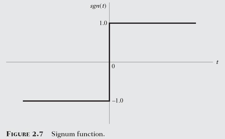
59 3. Sinusoidal Functions The Fourier transorm o the cosine unction cos( π t = c 1 [exp( jπ t + exp( jπ t] 1 cos( π ct [ δ ( c + δ ( + c (.70 The spectrum o the cosine unction consists o a pair o delta unctions occurring at =±c, each o which is weighted 1 by the actor ½ sin( π t [ δ ( δ ( + ] (.7 c c c j c c ] (.71 Fig Signum Function sgn( t = + 1, 0, 1, t t t > 0 = 0 < 0 Fig

60 Back Next Fig.15 60

61 Back Next Fig.16 61

62 This signum unction does not satisy the Dirichelt conditions and thereore, strictly speaking, it does not have a Fourier transorm exp( at, g( t = 0, exp( at, t > 0 t = 0 t < 0 (.73 Its Fourier transorm was derived in Example.3; the result is given by j4π G( = a + (π The amplitude spectrum G( is shown as the dashed curve in Fig..17(b. In the limit as a approaches zero, j4π F[sgn( t] = lim a 0 a + (π = 1 jπ sgn( t (.74 At the origin, the spectrum o the approximating unction g(t is zero or a>0, whereas the spectrum o the signum unction goes to ininity. 1 jπ Fig..17 6

63 Back Next 63

64 5. Unit Step Function The unit step unction u(t equals +1 or positive time and zero or negative time. 1, 1 u( t =, 0, t > 0 t = 0 t < 0 The unit step unction and signum unction are related by 1 u( t = [sgn(( t + 1] (.75 Unit step unction is represented by the Fourier-transorm pair The spectrum o the unit step unction contains a delta unction weighted by a actor o ½ and occurring at zero requency 1 1 u( t δ ( jπ + (.76 Fig

65 Back Next 65

66 6. Integration in the time Domain (Revisited The eect o integration on the Fourier transorm o a signal g(t, assuming that G(0 is zero. t y( t = g( τ dτ (.77 The integrated signal y(t can be viewed as the convolution o the original signal g(t and the unit step unction u(t y( t The Fourier transorm o y(t is = g( τ u( t τ dτ 1, τ < t 1 u( t τ =, τ = t 0, τ > t 1 1 Y ( = G( + δ ( j π (.78 66

67 67 The eect o integrating the signal g(t is ( (0 ( ( G G δ δ = ( (0 1 ( 1 ( G G j Y δ π + = (.79 ( (0 1 ( 1 ( G G j d g t δ π τ τ +

68 .5 Fourier Transorm o Periodic Signals A periodic signal can be represented as a sum o complex exponentials Fourier transorms can be deined or complex exponentials Consider a periodic signal g T0 (t gt ( t = cn exp( jπn0t 0 n= (.80 c n 1 = T 0 T 0 T / 0 / gt ( texp( jπn 0 0 t dt Complex Fourier coeicient 1 = 0 T 0 (.8 0 : undamental requency (.81 68

69 Let g(t be a pulselike unction g( t = gt 0, 0 ( t, T0 T0 t elsewhere (.83 g ( t = g( t mt0 0 T m= (.84 c n = ( exp( 0 g t = G( n 0 0 jπn 0 t dt (.85 gt ( t = 0 G( n0exp( jπn0t 0 n= (.86 69

70 One orm o Possisson s sum ormula and Fourier-transorm pair m= m= 0 n= g( t mt = G( n exp( j n t 0 0 π 0 0 n= g( t mt 0 G( n0 δ ( n0 (.87 (.88 Fourier transorm o a periodic signal consists o delta unctions occurring at integer multiples o the undamental requency 0 and that each delta unction is weighted by a actor equal to the corresponding value o G(n 0. Periodicity in the time domain has the eect o changing the spectrum o a pulse-like signal into a discrete orm deined at integer multiples o the undamental requency, and vice versa. 70

71 Fig

72 Back Next 7

73 73

74 .6 Transmission o Signal Through Linear Systems : Convolution Revisited In a linear system, The response o a linear system to a number o excitations applied simultaneously is equal to the sum o the responses o the system when each excitation is applied individually. Time Response Impulse response The response o the system to a unit impulse or delta unction applied to the input o the system. Summing the various ininitesimal responses due to the various input pulses, Convolution integral The present value o the response o a linear time-invariant system is a weighted integral over the past history o the input signal, weighted according to the impulse response o the system y( t = x( τ h( t τ dτ y( t = h( τ x( t τ dτ (.93 (.94 74

75 Back Next 75

76 76

77 Fig..1 77

78 Back Next 78

79 Causality and Stability Causality It does not respond beore the excitation is applied h( t = 0, t < 0 (.98 Stability The output signal is bounded or all bounded input signals (BIBO x( t < M or all t y( t = h( τ x( t τ dτ (.99 Absolute value o an integral is bounded by the integral o the absolute value o the integrand h( τ x( t τ dτ = M h( τ x( t τ dτ h( τ dτ y(t M h( τ dτ 79

80 A linear time-invariant system to be stable The impulse response h(t must be absolutely integrable The necessary and suicient condition or BIBO stability o a linear time-invariant system h( t dt < (.100 Frequency Response Impulse response o linear time-invariant system h(t, Input and output signal x( t = exp( jπt (.101 y( t = h( τ exp[ jπ ( t τ ] dτ = exp( jπt h( τ exp( jπτ dτ (.10 80

81 H ( = h( texp( jπt dt Eq. (.104 states that (.103 The response o a linear time-variant system to a complex exponential unction o requency is the same complex exponential unction multiplied by a constant coeicient H( An alternative deinition o the transer unction H ( y( t = H ( exp( jπt (.104 y( t = (.105 x( t = X ( exp( jπt d (.106 x( t x( t = exp( j πt x( t = lim X ( exp( j t ( π k = y( t = = = k lim 0 = k k = H ( X ( exp( jπt H ( X ( exp( jπt d (

82 The Fourier transorm o the output signal y(t Y ( = H ( X ( (.109 The Fourier transorm o the output is equal to the product o the requency response o the system and the Fourier transorm o the input The response y(t o a linear time-invariant system o impulse response h(t to an arbitrary input x(t is obtained by convolving x(t with h(t, in accordance with Eq. (.93 The convolution o time unctions is transormed into the multiplication o their Fourier transorms H ( = H ( exp[ jβ ( ] (.110 Amplitude response or magnitude response Phase or phase response H ( = H ( β ( = β ( 8

83 In some applications it is preerable to work with the logarithm o H( ln H ( = α ( + jβ ( (.111 α( = ln H ( (.11 ' α ( = 0log10 H ( (.113 The gain in decible [db] ' α ( = 8.69α ( (

84 Back Next 84

85 Paley-Wiener Criterion The requency-domain equivalent o the causality requirement α( 1+ d < (

86 .7 Ideal Low-Pass Filters Filter A requency-selective system that is used to limit the spectrum o a signal to some speciied band o requencies The requency response o an ideal low-pass ilter condition The amplitude response o the ilter is a constant inside the passband -B B The phase response varies linearly with requency inside the pass band o the ilter exp( jπt, 0 B B H ( = (.116 0, > B 86

87 Evaluating the inverse Fourier transorm o the transer unction o Eq. (.116 ( t = B exp[ jπ ( t t0 B h ] d (.117 h( t = sin[ jπb( t t π ( t t = B sin c[b(t - t 0 0 ] 0 ] (.118 We are able to build a causal ilter that approximates an ideal low-pass ilter, with the approximation improving with increasing delay t 0 sin c[b(t - t 0 ] << 1, or t < 0 87

88 88 Pulse Response o Ideal Low-Pass Filters The impulse response o Eq.(.118 and the response o the ilter ( τ π λ = t B (.119 sin c( ( Bt B t h = (.10 ( ] ( sin[ ] ( sin c[ ( ( ( / / / / τ τ π τ π τ τ τ τ τ d t B t B B d t B B d t h x t y T T T T = = = (.11 ]} / ( Si[ ] / ( {Si[ 1 sin sin 1 sin 1 ( / ( 0 / ( 0 / ( / ( T t B T t B d d d t y T t B T t B T t B T t B + = = = + + π π π λ λ λ λ λ λ π λ λ λ π π π π π

89 Sine integral Si(u sin Si( = u x u dx (.1 0 x An oscillatory unction o u, having odd symmetry about the origin u=0. It has its maxima and minima at multiples o π. It approaches the limiting value (π/ or large positive values o u. 89

90 The maximum value o Si(u occurs at u max = π and is equal to = (1.179 ( The ilter response y(t has maxima and minima at π T 1 tmax = ± ± B 1 y( t max = [Si( π Si( π πbt ] π 1 = [Si( π + Si(πBT π ] π π Odd symmetric property o the sine integral Si(πBT π = (1 ± Si( π = (1.179( π / y t ( max = ± ( ± 1 (.13 90

91 For BT>>1, the ractional deviation has a very small value The percentage overshoot in the ilter response is approximately 9 percent The overshoot is practically independent o the ilter bandwidth B 91

92 Back Next 9

93 Back Next 93

94 Back Next 94

95 Back Next 95

96 When using an ideal low-pass ilter We must use a time-bandwidth product BT>> 1 to ensure that the waveorm o the ilter input is recognizable rom the resulting output. A value o BT greater than unity tends to reduce the rise time as well as decay time o the ilter pulse response. Approximation o Ideal Low-Pass Filters The two basic steps involved in the design o ilter 1. The approximation o a prescribed requency response by a realizable transer unction. The realization o the approximating transer unction by a physical device. the approximating transer unction H (s is a rational unction H ' ( s = H ( j π = ( s z1( s = K ( s p ( s 1 s z ( s zm p ( s p n Re([ pi ] < 0, or all i 96

97 Minimum-phase systems A transer unction whose poles and zeros are all restricted to lie inside the let hand o the s-plane. Nonminimum-phase systems Transer unctions are permitted to have zeros on the imaginary axis as well as the right hal o the s-plane. Basic options to realization Analog ilter With inductors and capacitors With capacitors, resistors, and operational ampliiers Digital ilter These ilters are built using digital hardware Programmable ; oering a high degree o lexibility in design 97

98 .8 Correlation and Spectral Density : Energy Signals Autocorrelation Function Autocorrelation unction o the energy signal x(t or a large τ as R x The energy o the signal x(t * ( τ = x( t x ( t τ dτ (.14 The value o the autocorrelation unction Rx(τ or τ=0 R x (0 = x( t dt 98

99 Energy Spectral Density The energy spectral density is a nonnegative real-valued quantity or all, even though the signal x(t may itsel be complex valued. Ψ x ( = X ( (.15 Wiener-Khitchine Relations or Energy Signals The autocorrelation unction and energy spectral density orm a Fouriertransorm pair Ψ x ( = R x ( τ exp( jπτ dτ (.16 R x ( τ = Ψ ( exp( j d x π τ (.17 99

100 1. By setting =0 The total area under the curve o the complex-valued autocorrelation unction o a complex-valued energy signal is equal to the real-valued energy spectral at zero requency. By setting τ=0 R x ( τ dτ = Ψ (0 x The total area under the curve o the real-valued energy spectral density o an erergy signal is equal to the total energy o the signal. Ψ x ( d = R (0 x 100

101 101

102 Eect o Filtering on Energy Spectral Density When an energy signal is transmitted through a linear time-invariant ilter, The energy spectral density o the resulting output equals the energy spectral density o the input multiplied by the squared amplitude response o the ilter. Y ( = H ( X ( Ψ ( y = H ( Ψ (.19 An indirect method or evaluating the eect o linear time-invariant iltering on the autocorrelation unction o an energy signal 1. Determine the Fourier transorms o x(t and h(t, obtaining X( and H(, respectively.. Use Eq. (.19 to determine the energy spectral density Ψ y ( o the output y(t. 3. Determine R y (τ by applying the inverse Fourier transorm to Ψ y ( obtained under point. x ( 10

103 Fig

104 Back Next 104

105 Fig

106 Back Next 106

107 Fig

108 Back Next 108

109 109 Interpretation o the Energy Spectral Density The ilter is a band-pass ilter whose amplitude response is The amplitude spectrum o the ilter output The energy spectral density o the ilter output + = (.134 otherwise 0, 1, ( H c c Fig = = (.135 otherwise 0,, ( ( ( ( X X H Y c c c + Ψ = Ψ (.136 otherwise 0,, ( ( c c c x y

110 Back Next 110

111 The energy o the ilter output is E y = Ψ y ( d = Ψ ( d 0 y The energy spectral density o an energy signal or any requency The energy per unit bandwidth, which is contributed by requency components o the signal around the requency E y Ψ ( x c (.137 Ψ x ( c E y (.138 Fig

112 Cross-Correlation o Energy Signals The cross-correlation unction o the pair R xy The energy signals x(t and y(t are said to be orthogonal over the entire time domain I R xy (0 is zero * ( τ = x( t y ( t τ dt x( t y ( t dt = 0 The second cross-correlation unction R yx * (.140 * ( τ = y( t x ( t τ dt * R xy ( τ R ( τ = yx (.14 (.139 (

113 The respective Fourier transorms o the cross-correlation unctions R xy (τ and R yx (τ Ψ Ψ xy yx ( = R ( τ exp( jπτ dτ xy ( = R ( τ exp( jπτ dτ yx (.143 (.144 With the correlation theorem Ψ xy ( = X ( Y * ( (.145 Ψ yx ( = Y ( X * ( (.146 The properties o the cross-spectral density 1. Unlike the energy spectral density, cross-spectral density is complex valued in general.. Ψ xy (= Ψ * yx( rom which it ollows that, in general, Ψ xy ( Ψ yx ( 113

114 .9 Power Spectral Density The average power o a signal is 1 T P = lim T x( t dt (.147 T T P < Truncated version o the signal x(t x T t ( t = x( trect T x( t, T t T = 0, otherwise (.148 x T ( t X ( T 114

115 The average power P in terms o x T (t 1 P = lim x ( t dt (.149 T T T 1 P = lim X ( d (.150 T T T x T ( t 1 S x ( = lim X ( (.15 T T T The total area under the curve o the power spectral density o a power signal is equal to the average power o that signal. P = S ( d (.153 dt = X ( d 1 P = lim X ( d (.151 T T T T Power spectral density or Power spectrum x 115

116 116

117 117

118 .10 Numerical Computation o the Fourier Transorm The Fast Fourier transorm algorithm Derived rom the discrete Fourier transorm Frequency resolution is deined by = N 1 NT s = = s 1 T (.160 Discrete Fourier transorm (DFT and inverse discrete Fourier transorm o the sequence g n as g = n g ( nts (.161 G g k n N 1 = n= 0 g N 1 = N = k n 1 0 jπ exp kn, N G k jπ exp kn, N k = 0,1,..., N 1 n = 0,1,..., N 1 (.16 (

119 Interpretations o the DFT and the IDFT For the interpretation o the IDFT process, We may use the scheme shown in Fig..34(b exp jπ kn N π = cos kn + N π jsin kn N π π = cos kn,sin kn, N N k = 0,1,..., N 1 (.164 At each time index n, an output is ormed by summing the weighted complex generator outputs Fig

120 Back Next 10

121 Back Next 11

122 Fast Fourier Transorm Algorithms Be computationally eicient because they use a greatly reduced number o arithmetic operations Deining the DFT o g n G k N 1 = n= 0 g n W nk, k = 0,1,..., N 1 (.165 jπ W = exp (.166 N W ( k + ln ( n+ mn W W N N / = W = exp( jπ = 1 = exp( jπ = 1 kn, or L N = m, l = 0, ± 1, ±,... 1

123 13 We may divide the data sequence into two parts For the case o even k, k=l, ( ,1,...,, ( 1 / ( 0 / / 1 / ( 0 / ( / 1 / ( 0 1 / 1 / ( 0 = + = + = + = = + = + + = = = N k W W g g W g W g W g W g G kn N n kn N n n N n N n k N n N n nk n N N n nk n N n nk n k k kn W 1 ( / = (.168 N / n n n g g x + + = ( ,1,...,, ( 1 / ( 0 ln = = = N l W x G N n n l = = / exp 4 exp N j N j W π π

124 For the case o odd k y n = gn gn+ N / N k = l + 1, l = 0,1,..., 1 (.170 G l+ 1 = = ( N / 1 ( N n= 0 / n= 0 y 1 n W [ y W n (l+ 1 n n ]( W ln, l = 0,1,..., N 1 (.171 The sequences xn and yn are themselves related to the original data sequence Thus the problem o computing an N-point DFT is reduced to that o computing two (N/-point DFTs. Fig

125 Back Next 15

126 Back Next 16

127 Important eatures o the FFT algorithm 1. At each stage o the computation, the new set o N complex numbers resulting rom the computation can be stored in the same memory locations used to store the previous set.(in-place computation. The samples o the transorm sequence G k are stored in a bit-reversed order. To illustrate the meaning o this latter terminology, consider Table. constructed or the case o N=8. Fig

128 Back Next 18

129 Computation o the IDFT Eq. (.163 may rewrite in terms o the complex parameter W g n N 1 = N k = 1 0 G W k kn, n = 0,1,..., N 1 (.17 Ng * n N 1 = k = 0 * kn G W k, 0,1,..., N 1 (

130 .11 Theme Example : Twisted Pairs or Telephony Fig..39 The typical response o a twisted pair with lengths o to 8 kilometers Twisted pairs run directly orm the central oice to the home with one pair dedicated to each telephone line. Consequently, the transmission lines can be quite long The results in Fig. assume a continuous cable. In practice, there may be several splices in the cable, dierent gauge cables along dierent parts o the path, and so on. These discontinuities in the transmission medium will urther aect the requency response o the cable. Fig

131 We see that, or a -km cable, the requency response is quite lat over the voice band rom 300 to 3100 Hz or telephonic communication. However, or 8-km cable, the requency response starts to all just above 1 khz. The requency response alls o at zero requency because there is a capacitive connection at the load and the source. This capacitive connection is put to practical use by enabling dc power to be transported along the cable to power the remote telephone handset. It can be improved by adding some reactive loading Typically 66 milli-henry (mh approximately every km. The loading improves the requency response o the circuit in the range corresponding to voice signals without requiring additional power. Disadvantage o reactive loading Their degraded perormance at high requency Fig

132 Back Next Fig

133 .1 Summary and Discussion Fourier Transorm A undamental tool or relating the time-domain and requency-domain descriptions o a deterministic signal Inverse relationship Time-bandwidth product o a energy signal is a constant Linear iltering Convolution o the input signal with the impulse response o the ilter Multiplication o the Fourier transorm o the input signal by the transer unction o the ilter Correlation Autocorrelation : a measure o similarity between a signal and a delayed version o itsel Cross-correlation : when the measure o similarity involves a pair o dierent signals 133

134 Spectral Density The Fourier transorm o the autocorrelation unction Cross-Spectral Density The Fourier transorm o the cross-correlation unction Discrete Fourier Transorm Standard Fourier transorm by uniormly sampling both the input signal and the output spectrum Fast Fourier transorm Algorithm A powerul computation tool or spectral analysis and linear iltering 134

135 Thank You!