Perturbations in Boolean Networks

Transcription

1 Perturbations in Boolean Networks as Model of Gene Regulatory Dynamics Von der Fakultät für Mathematik und Informatik der Universität Leipzig angenommene Dissertation zur Erlangung des akademischen Grades Doctor rerum naturalium (Dr. rer. nat.) im Fachgebiet Informatik vorgelegt von M. Sc. Physics Fakhteh Ghanbarnejad geboren am 2. September 1984 in Teheran Die Annahme der Dissertation wurde empfohlen von: 1. Prof. Dr. Peter F. Stadler (Leipzig, Deutschland) 2. Prof. Dr. Olli Yli-Harja (Tampere, Finnland) Die Verleihung des akademischen Grades erfolgt mit Bestehen der Verteitigung am mit dem Gesamtprädikat magna cum laude.

2

3 To my parents

4

5 Contents Abstract Acknowledgments ix xi 1 Introduction Gene Regulatory Dynamics Mathematical Formalisms Continuous Models Discrete Models Computational Aspects Structure of the Thesis Boolean Networks: Mathematical Framework Graph Dynamics Boolean Functions Updating Schemes Attractors Ensembles of Random Boolean Networks Critical Boolean Networks Boolean vs. Continuous Dynamics Empirical Boolean Networks Noise in Gene Regulatory Dynamics The Nature of Noise Mathematical formalisms and Fluctuations v

6 3.3 Discussion Dynamical Impact of Individual Nodes in Boolean Networks Introduction Dynamical Impact Results for Random Boolean Networks Switching Between Attractors Dynamical Impact in Real Boolean Networks Ranking Strategies and Continuous Boolean Dynamics Discussion Methods Stability of Boolean Dynamics Introduction Small Perturbations Fixed points and bistable circuits Stability of (3, 2) Boolean Networks Stability in random networks Discussion Methods Stabilizing of Boolean Dynamics Introduction Boolean Networks with Distributed Delays Cumulated Hamming Distance Results and Discussion Summary and Outlook 67 A Algorithms 69 A.1 Function Probabilities in Maximum Entropy Ensemble A.2 Boolean Attractors A.3 Continuous Dynamics A.4 Estimation of Dynamical Impact A.5 Eigenvector A.6 Ranking List of Figures 77 List of Tables 79 vi

7 Bibliography 81 vii

8 viii

9 Abstract Boolean networks are coarse-grained models of the regulatory dynamics that controls the survival and proliferation of a living cell. The dynamics is time- and state-discrete. This Boolean abstraction assumes that small differences in concentration levels are irrelevant; and the binary distinction of a low or a high concentration of each biomolecule is sufficient to capture the dynamics. In this work, we briefly introduce the gene regulatory models, where with the advent of system-specific Boolean models, new conceptual questions and analytical and numerical challenges arise. In particular, the response of the system to external intervention presents a novel area of research. Thus first we investigate how to quantify a node s individual impact on dynamics in a more detailed manner than an averaging against all eligible perturbations. Since each node now represents a specific biochemical entity, it is the subject of our interest. The prediction of nodes dynamical impacts from the model may be compared to the empirical data from biological experiments. Then we develop a hybrid model that incorporates both continuous and discrete random Boolean networks to compare the reaction of the dynamics against small as well as flip perturbations in different regimes. We show that the chaotic behaviour disappears in high sensitive Boolean ensembles with respect to continuous small fluctuations in contrast to the flipping. Finally, we discuss the role of distributing delays in stabilizing of the Boolean dynamics against noise. These studies are expected to trigger additional experiments and lead to improvement of models in gene regulatory dynamics. ix

10 x

11 Acknowledgments I would like so simply just say, thank you! Konstantin Klemm Peter F. Stadler My beloved mother, father and Hadi Mona D. Jens, Petra The beerinformaticians Atefeh, Fatemeh S., Florian, Ghazaleh, Gunnar, Ida, Mahboubeh, Maribel, Mina, Mohammad, Mona H., Nadjieh, Nasim, Roghayeh, Sima, Shahin, Wolfgang,... All my teachers and professors and all the people who have influenced my thinking xi

12 xii

13 CHAPTER 1 Introduction Once upon a time, a little boy was looking for something under a street light. What are you looking for? asked an old man passing by. My key he replied. Where have you lost it?! He asked while looking around confusedly. In that dark area over there said the boy pointing to an area meters away. So why are looking for it here?!! said the old man surprisedly. Because there is light over here! replied the boy. What scientists do based on a tale I heard in a Critical Phenomena class taught by Prof. Shahin Rohani The functioning of organisms on the molecular level is a research topic of increasing attention. Survival and reproduction requires an autonomous regulation of chemical concentrations in the living cell. In this chapter we open our discussions with an introduction to gene regulatory dynamics, the applied and developed mathematical formalisms and computational aspects. 1.1 Gene Regulatory Dynamics The first discovery of a gene regulation system was done in 1961 by Jacob and Monod [1]. They found that some enzymes involved in lactose metabolism are expressed by the genome of E. coli only in the presence of lactose and absence of glucose. The importance of gene regulations for living cells in order to increase the versatility and adaptability of an organism has since triggered a central attention of researchers in this area. 1

14 Introduction For introducing the genetic regulatory systems, Hidde De Jing starts his review paper [2] by the following words: In order to understand the functioning of organisms on the molecular level, we need to know which genes are expressed, when and where in the organism, and to which extent. The regulation of gene expression is achieved through genetic regulatory systems structured by networks of interactions between DNA, RNA, proteins, and small molecules. He continues to make a general picture of such systems by addressing gene expression as follows: Gene expression is a complex process regulated at several stages in the synthesis of proteins [3]. Apart from the regulation of DNA transcription, the best-studied form of regulation, the expression of a gene may be controlled during RNA processing and transport (in eukaryotes), RNA translation, and the posttranslational modification of proteins. The degradation of proteins and intermediate RNA products can also be regulated in the cell. The proteins fulfilling the above regulatory functions are produced by other genes. This gives rise to genetic regulatory systems structured by networks of regulatory interactions between DNA, RNA, proteins, and small molecules. An example of a simple regulatory network, involving three genes that code for proteins inhibiting the expression of other genes, is shown in Fig Proteins B and C independently repress gene a by binding to different regulatory sites of the gene, while A and D interact to form a heterodimer that binds to a regulatory site of gene b. Binding of the repressor proteins prevents RNA polymerase from transcribing the genes downstream. Certain reasons make the understanding and modeling of the regulatory systems a hot research topic. The first one is their entanglement with the complexity concept. After finding the lack of correlation between genome size and complexity, known as the C-value paradox [4], as well as between the number of genes and complexity, known as the G-value paradox [5], the paradigm of complexity of organisms has been shifting to the complexity of the regulatory control structures where for example various combinations of genes might allow up to different gene expression patterns [6]. The second outstanding point which is motivating scientists to study such dynamics is their relevance to the evolution which occurs with genetic variability and could be understood in the context of regulations [7]. Recent works point to the key roles that regulatory changes could play in evolutionary processes e.g. in primate evolution [8] or the evolution of human and chimpanzee transcriptome [9]. And the last but not the least motivation to investigate these systems is also their possible relevance to the cause and treatment of cancer [10, 11, 12]. 2

15 1.2 Mathematical Formalisms Figure 1.1: Example of a genetic regulatory system, consisting of a network of three genes a, b, and c, repressor proteins A, B, C, and D, and their mutual interactions. The figure distinguishes several types of interaction. The figure and the caption is adopted from Ref. [2]. 1.2 Mathematical Formalisms Different mathematical formalisms and numerical methods have been used for modelling such regulatory dynamics. These models deal with different levels of information, complexity and computational expenses. Classifying available models in the different levels (see figure 1.2) Bornholdt tries to develop a general intuition that how to build a fit model for large genetic networks [13]; What details can be ignored without being unfaithful to the general behaviour of the system? Which element can be considered as the building block of the model? Which parameters are ignorable while the others are vital in our modelling? These are questions that he addresses to review the history of modeling of gene regulatory systems and extrapolate the best option for the levels not reached yet (right column in Fig. 1.2) [13]. Here we focus on two main classes of models: small genetic circuit and mid-size genetic network models as shown schematically in the figure 1.2, center left column and center right column respectively. In this point of view, various mathematical approaches have been developed, from discrete to continuous methods, from deterministic to stochastic techniques, from static to dynamical models, from detailed and fine to coarse grained perspectives; Let us take a more detailed look at the well-structured review paper [2] and rewrite it in our own words. Here we re-sort some of the reviewed models according to their dynamical state details whether they are continuous or discrete as listed in the table 1.1, since we need this perspective in later chapters 1. 1 We are not discussing all of these models in details, As we merely want to create a general image from the 3

16 Stefan Bornholdt cellular machinery that regulates the activity of a gene. When at least a few tens of molecules are involved in regulating a gene, details of the interactions can usually be neglected, and interaction rates can be used instead of tracking the single molecular binding events (2). With large networks involving thousands of regulatory genes (genes that encode proteins that regulate other genes), the number of differential equations needed to describe the system can become huge. The sheer number of parameters (such as decay rates, production rates, and interaction strengths) in this mathematical model poses a chal- r is with the Instiheoretical Physics, y of Bremen, Ottoe, D Bremen, bornholdt emen.de Gene activity Proteins he biology of information process- tial equations approach, the authors find g in the living cell shifts from the that the intricate internal dynamics of a fredy of single signal Introduction transduction quent cellular subcircuit exhibits a simple to increasingly complex regula- bistable ON/OFF behavior, and thus works, mathematical models could be modeled by something much simndispensable tools. Detailed pre- pler than differential equations something models of large genetic networks as simple as a switch. olutionize how researchers study A f irst level of coarse-graining in diseases, yet such models are not genetic regulation already exists in the n reach. One reason is that experi- standard approach of modeling protein and data for large systems are inlow System complexity High e; another is that Single gene Small genetic circuit Mid-size genetic network Large genetic network etic systems are to model. Extrathe standard difequations model A Out B le gene (with its kinetic paramelarge systems nder the model vely complicated. ible way to simgreat detail Computer modeling Less detail h models would nd a coarsediscrete dynamics Stochastic molecular Differential equations Pseudodynamics (connected switches) simulations (flow across a network) level of descripenetic networks; focus on the sysd[rna] αkh = avior of the netdt kh + [Protein(t-τ)] hile neglecting d[protein] ar details wher= β[rna(t)] dt ible (see the figin Out ch an approach r other fields of Single gene dynamics Information System dynamics for example, the of molecular Flow pattern of network states Functional modules n organic chemhich mercifully from the details X derlying quantum Y On page 496 in, Brandman et al. s to the possibiltime Time mplifying large network models. tandard differen- The different levels of description in models of genetic networks. Whereas single genes can be modeled in molec- ular detail1.2: with stochastic simulations (leftof column), a differentialmodelling equation representation of gene dynamics is more Figure The different levels mathematical for gene regulatory networks. practical when turning to circuits of genes (center left column). Approximating gene dynamics by switchlike ON/OFF While stochastic simulations can present single genes in molecular detail (left column), modbehavior allows modeling of mid-sized genetic circuits (center right column) and still faithfully represents the overall elling circuits genes system. with differential applicative (center left column). By dynamics of the of biological Large geneticequation networks is aremore currently out of reach for predictive simulations. turning to mid-sized genetic such circuits switch-like ON/OFF dynamical models faithfully However, more simplified dynamics, as percolating flows across a network structure, can teach uscan about the functional structure a large network (right column). reproduce theofgeneral behaviour of the system (center right column). We should take lessons from percolating flows across a network structure in terms of how to model a larger genetic SCIENCE 21 OCTOBER 2005 from Ref. [13]. network (right column). The figure VOL and 310 the caption is adopted Published by AAAS 4 Downloaded from on April 4, 2012 Genetic Networks

17 1.2 Mathematical Formalisms Table 1.1: Ref. [2]. Continuous and discrete models of gene regulatory systems. Table is taken from Models Discrete(d), Continuous(c) Nonlinear Differential Equations (NLDE) c Piecewise-Linear Differential Equations (PLDE) c Directed Graphs (DG) 1 Boolean Networks (BN) d Generalized Logical Networks (GLN) d Stochastic Master Equations (SME) d 1 This is a static model, so there is no dynamics to be continuous or discrete Continuous Models The common approach to model a typical dynamical system in science and engineering is ordinary differential equations (ODE). They were applied to study biological regulatory systems as well, where solutions represent the continuous values of concentrations x i of genes, RNAs, proteins or other types of molecules. In other words, the models give us the rate of productions of the biochemical elements as a function of time which is given by the general equation 1.1. dx i (t) dt = f i (x(t)) i {1,..., N} (1.1) when f i : R N R is a suitable linear, nonlinear or piece-wise linear function. Dealing with circuits of genes, this kind of modelling is more practical than detailed single genes models [13]. Nonlinear Ordinary Differential Equations In most cases, the best fit choice in Eq. 1.1 is a nonlinear function (nonlinear differential equations - NLDE); and sometimes equations include some time delays representing the time that the system needs to pass the information or materials from one element to the other by transcriptions, translations, diffusions or other transporting processes in the system (delay differential equations - DDEs). E.g. the oscillations of protein Hes1 were reproduced by Eq Connection of this protein to cell differentiation made it an important and interesting case to study [14]. applied and developed mathematical models in the field of regulatory systems in the direction needed in the later discussions. Please read the reference [2] and its references for more models, technical details and examples. 5

18 Introduction Figure 1.3: An example of s-shaped curve. The plot represents following function, x = 1 1+exp t t ( 10, 10) d[mrn A] d[t] d[hes1] d[t] = αk h k h + [Hes1(t τ)] h [mrna(t)] τ rna (1.2) = β[mrna(t)] [Hes1(t)] τ hes1 Where the parameters τ, α, k, h, τ hes1, τ rna denote production delay, production rates, characteristic concentration, binding threshold h which is the Hill coefficient and characteristic degradation times respectively. Piecewise-Linear Differential Equations To simplify qualitative analysis, let us consider the switching behaviour of the biological components from lowest concentration values to the highest rates or vice versa by continuous s-shaped curves which are known as sigmoid functions (one of them is shown in Fig. 1.3). The mathematical properties of this type of functions and the mapped biological dynamics were studied in Ref. [15]. So this simplification provides piecewise-linear differential equation (PLDE) models formulated in the general form 1.3; which make us ready to work on later abstract discrete models such as Boolean networks and generalized logical networks. dx i (t) dt = g i (x(t)) γ i x i i {1,..., N}, γ i > 0 (1.3) where x i plays the role of the production value of gene i and γ denotes its degradation rate. Here the f function in Eq. 1.1 is replaced by the piece-wise linear function g i (x(t)) γ i x i. 6

19 1.2 Mathematical Formalisms d[x j (t)] d[t] = g j (x j 1 (t τ)) x j (t) with (1.4) g j (x i ) = η j 1 + d j i xν i τ 1+b j i xν i Equation 1.4 denotes a theoretically-studied example of circuits with PLDE [16] Discrete Models Despite the fact that the first group of models studied here have been in good agreement with detailed experimental databases, some problems should be taken in the account. On the one hand, the point is that usually it s not possible to find an exact, analytical solution to the equations, due to the presence of the nonlinear terms. Thus the numerical methods give us a chance to make an approximation to the behaviour of the dynamics, find the steady states and test the stability of them. Figure 1.4: An example of mid-size regulatory genetic network in the sea urchin embryos. See Ref. [17] for details and this figure. On the other hand, one should note the large number of parameters needed to reproduce the dynamics of just one single gene, as seen in the above example of equation 1.2. The high computational costs associated with the modelling of larger regulatory systems (such as 7

20 Introduction V = {1,2} E = {<1,2,+>,<1,1,+>,<2,1,->,<2,2,->} Figure 1.5: A simple directed graph. In the set E denotes that gene i activates gene j and < i, j, > denotes that i is inhibiting j. the one shown in figure 1.4) has led to the simplification of models. Therefore going from small genetic circuit to mid-size genetic network, a transition happened in modelling, from continuous to discrete models. Moreover, some studies have shown that such models are quite stable to represent and predict the overall behaviour of the system against variations of kinetic parameters over several orders of magnitude [14]. This was yet another important fact that encouraged modellers to transition to another level of modelling and focus their attention to the structure of the interactions more than precise values of the parameters; Thus messy parametric models have been replaced by models with much fewer parameters or even parameterless models. Directed Graphs Mapping the interactions between the elements of the regulatory system like genes or proteins to a directed graph (DG) provides us with a static model, where edges tell us which element influences which other elements. Type of information that edges can carry is whether one element is activating or inhibiting the others, which is shown by a simple sign +/, respectively. Figure 1.5 shows an example of a directed graph G defined by < V, E >; When V presents set of nodes and E shows set of interactions. These graphs can be obtained by various approaches. One might directly compose the graph from databases or use reverse engineering methods. Analyzing the mathematical characters of the mapped graph provides some information about the original biological data. For instance, cycles in the graph indicate feedback relations. The average and the distribution of the interactions give us an estimation of the complexity of the system and so on. Boolean Networks Boolean networks (BN)[18, 19, 20, 21, 22, 23] is another framework for modeling regulatory systems, especially for precise sequence control as observed in morphogenesis [24] and cell cycle dynamics [25] but also in the regulation of the metabolism [26]. An N-dimensional Boolean map f : {0, 1} N {0, 1} N gives rise to a time-discrete dynam- 8

21 1.2 Mathematical Formalisms -1 A -1-2 B -2 x1x2 fa fb Figure 1.6: An example of generalized logical networks. Edge labels show which thresholds should be taken, the signs indicate inhibitors and excitatories and specified logical rules are written in the table. ics x(t + 1) = f(x(t)) (1.5) with x = (x 1,..., x N ) being a Boolean state vector (bit string) of N entries. Such a map is equivalent to a Boolean network. When f is pictured as a network, a node corresponds to a coordinate i of the Boolean state vector and a directed edge j i (from node j to node i) is present if the Boolean function f i explicitly depends on the j-th coordinate. The main idea behind these types of modeling is that we can ignore the intermediate expression levels of genes and consider them as occupying either of two states of active (on, 1) or inactive (off, 0) at any given time. See chapter 2 for further detailed discussions. Generalized Logical Networks To generalize Boolean networks, one can consider variables with more than two values. The extension has been developed in different directions; However we only describe the main idea of generalization by the following formalism [27]. Let us consider p+1 state values. In this case, the continuous concentration rates are mapped to the abstract state values, x i {0, 1, 2,..., p} according to the defined thresholds, θ 1 i < θ2 i <... < θp i written in equation 1.6. x i = 0, if x i < θi 1 (1.6) x i = 1, if θi 1 x i < θi 2... x i = p, if x i θ p i and dynamics still follows the equation 1.5, but f is a more complicated logical rule, f : {0, 1,..., p} N {0, 1,..., p} N. Figure 1.6 indicates a simple example of generalized logical 9

22 Introduction networks (GLN). The graph has two nodes which are regulated by the other node states, first input, and their own states, second input, in the last time step. The system has three thresholds which means states have three possible values, x i {0, 1, 2}; So the state space includes (p + 1) N = 3 2 = 9 states and logical functions, generalized Boolean functions, can be chosen from (p + 1) (p+1)n = 3 32 = possibilities and should be consistent with imposed restrictions of the thresholds. Edges are labelled with the rank number of thresholds, while the signs show whether the regulations are excitatory or inhibitory. e.g. 2 means that node A is an inhibitor of node B and influences it above its second threshold. The functions, f A = f(x B, x A ), f B = f(x A, x B ) are specified in the right hand table of figure. Since the dynamics is deterministic and state space is finite, as are the Boolean networks, any initial condition ends to a logical steady state or cycle; These steady states could correspond to the patterns of gene expression [28]. Stochastic Master Equations Since some assumptions of the continuous and deterministic approaches may be questionable according to the nature of the regulatory phenomena, discrete and stochastic models were proposed as another alternative (see Ref. [2] and its references). Eq. 1.7 presents a general form of such models; where the discrete variable X refers to the molecules states, p(x, t) indicates the probability that at time t the cell contains a given amount of different molecules of X 1, X 2,... ; m is the number of the chemical reactions making the dynamics, β j is the probability that reaction j bring the system from another state to the current state X while α j p(x, t) is the probability that reaction j is in the state X at time t. Thus the stochastic master equation (SME) 1.7 gives the time evolution of the joint probability distribution p(x, t). p(x, t) t m = [β j α j p(x, t)] (1.7) j=1 1.3 Computational Aspects Let us summarize what we said so far. We introduced the biological phenomena which we are trying to understand and model; Then we reviewed the most widely used and developed mathematical formalisms mapped to them. Now let us speak a bit about the limitations and problems in these two realms, i.e. experiment and theory. On the one hand, sometimes to setting up an experiment is not very easy because of various shortages such as lack of technological facilities, expenses, etc.; or there are some problems in the later stages such as storing of a huge body of empirical data and further analysing the stored databases statistically. On the other hand, mapping a mathematical formalism to the laboratory observations which is able to explain the phenomena in the language of precise numbers is not a very easy and simple task. Also whenever the mathematical model seems to fit the data, its predic- 10

23 1.3 Computational Aspects Figure 1.7: The computational bridge between experiment and theory, the external world and human internal world, in the natural sciences. In the last century scientists were equipped by computers to shorten the gap between laboratory and mind worlds. tions should be tested; But how can we confirm the theory where experiment is not possible? Would that be the end of the story? Of course not! Here is where computational approaches come into play. Simulations try to provide the missing link between experiment and theory in all different levels of natural sciences, Fig Although computational methods struggle with their own limitations, borders, costs and difficulties, numerical results provided by them can make outlines for theoreticians as well as experimentalists in terms of where to search for what, thereby reducing the costs and speeding up the research projects to achieve the goals more efficiently. Our approach in this thesis is computational and aims at assessing the limitations and power of mathematical models mapping gene regulatory systems. From this point of view, we do specifically focus on Boolean dynamics and particularly perturbations on dynamics, since Boolean networks are good candidates for modelling regulatory dynamics and enable us to pass from one level of modelling to the larger system sizes [13]. Let us go back to our main concern, namely the study of gene regulatory systems, and revisit it now by a computational gloss to understand what makes Boolean networks specific in term of computations. We try to find similarities between the regulatory systems and a simple washing machine which we work with daily 2. Thus there are two outstanding lessons from computer engineering which give us hints as to how to improve our methods. First, a washing machine has a designed control circuit which receives some input data like temperature, water level, switches, etc; and after analyzing it makes an output including a sequence of instructions to tune the temperature, water level and so on. Similarly we can reduce our model to a dynamics including a series of molecular activations which regulates the cell cycle elements such as cell size, temperature, stress, food supply and so on, in response to the received input information e.g. damage, food sources and supply, light and any other internal or external data or stimuli. Second, we need to know how to build up this sequence in 2 This example is adopted from Ref. [29] 11

24 Introduction mathematical language. Which details must be considered in the dynamics and which are not necessary? Since the machine alphabet is binary, a good option is a binary dynamics which can represent the dynamical actions (or reactions) by a sequence of the involved gene states (0s and 1s) ignoring the switching details. These models are the ones which we know as Boolean networks. 1.4 Structure of the Thesis What motivates us to study the models properties, discussed in section 1.2, is a better mathematical understanding of gene regulatory systems explained in Sec. 1.1; Finally in the section 1.3 we tried to address, very briefly, the main idea behind the computational aspects which could help us improve the mathematical frameworks and enable us to find out the limitations and problems of the developed models. In this thesis, we study the role of perturbations in Boolean networks as a model of gene regulatory dynamics. Hence first we introduce the mathematical framework of Boolean networks in chapter 2. Then we review in chapter 3 the nature of noise in regulatory systems and studies of different types of fluctuations in mathematical formalisms. In chapter 4, we make centrality measures based on topological as well as dynamical characters of the Boolean networks to rank nodes with respect to their capability to spread perturbations on dynamics. The chapter is based on the following preprint paper: Ghanbarnejad F, Klemm K (2011). Impact of individual nodes in Boolean network dynamics, Europhysics letters (resubmitted after minor revision, 2012), in preprint arxiv: v1. In chapter 5, we investigate the dynamical resilience of random Boolean networks against flip perturbations and small perturbations. The chapter is based on the following publication: Ghanbarnejad F, Klemm K (2011). Stability of Boolean and continuous dynamics, Phys. Rev. Lett In chapter 6, we study spreading of flip perturbations on dynamics updated synchronously according to the nodes flat distributed delays. Finally we summarize our take home messages in chapter 7. The appendix A presents some technical tricks in the simulations. 12

25 CHAPTER 2 Boolean Networks: Mathematical Framework Mathematics is the art of giving the same name to different things. Jules Henri Poincare ( ) A Boolean network is a state- and time-discrete dynamical system. The dynamics is defined by an iteration x(t + 1) = f(x(t)) (2.1) with N Boolean dynamical variables written as a binary vector x(t) {0, 1} N at each time t N {0}. The mapping f : {0, 1} N {0, 1} N is typically sparse: calculating the state x j (t + 1) requires knowledge of the state x i (t) for a few ( N) indices i at the previous time step. When the system is pictured as a directed network, the nodes {1, 2,..., N} carry the dynamic variables x 1, x 2,..., x N interacting along a relatively small number of directed arcs. Subindices address components of a vector such that x j is the Boolean state of node j and f j is its Boolean function. In order to formalize and quantify these ideas, we consider the x i -dependence of f as the mapping { (i) 1 if f j (x) f j (x i ) f j (x) = (2.2) 0 otherwise This is the Boolean analogue of the usual partial derivative of a function, using x i to denote state vector x with its i-th entry negated. Note that (i) f also maps from {0, 1} N to {0, 1} N. 13

26 Boolean Networks: Mathematical Framework A A A B B B B A Figure 2.1: A (2, 1) Boolean network can have 4 different topologies presented above. By averaging (i) f over all states with equal weight, the activity of i on j is obtained as α ij (f) = 2 N (i) f j (x) (2.3) x {0,1} N The activity α ij (f) is the probability that a perturbation (negation of state) at node i causes a perturbation at node j in the subsequent time step, assuming that all 2 N state vectors occur with equal probability. The sensitivity of the Boolean function f i is the sum of its incoming activities, N s i (f) = α ji. (2.4) Likewise, we define the strength of f i as the sum of outgoing activities [32] N σ i (f) = α ij. (2.5) Any random Boolean network is unique by its specified topology (Sec. 2.1) and dynamical rules (Sec. 2.2). j=1 j=1 2.1 Graph The directed network on the nodes {1, 2,..., N} obtained from f contains an arc from node i to node j if and only if α ij (f) 0. The adjacency matrix A of the network has an entry a ij = 1 if α ij (f) 0 and a ij = 0 otherwise. An N-node network can have various topologies based on different in-degree and out-degree probability distributions. Restricting all nodes to receive K inputs leads to the flat probability distribution function, P in = K N, and therefore a Poisson distribution of out-degree, P out(k) = K k k! e K, in the limit of N [21]. These Boolean networks are known as (N, K). Figure 2.1 presents 4 possible (2, 1) Boolean networks; Another alternative for in- or out-degree k distribution is power law, P (k) = P γ kmax, which is well-known for biological networks [33] i=k k γ min 14

27 2.2 Dynamics Table 2.1: Different possible Boolean functions corresponding to 1 input(up) and 2 inputs(down). The functions can be classified in 3 groups: a) reversible like f 1, f 2, F 6, F 9 where the output changes by changing an input b) frozen like f 0, f 3, F 0, F 15 where the output is constant independent of its inputs c) canalizing like the rest of the functions which have a fixed output corresponding to the value of canalizing input regardless of the other inputs In f 0 f 1 f 2 f In F 0 F 1 F 2 F 3 F 4 F 5 F 6 F 7 F 8 F 9 F 10 F 11 F 12 F 13 F 14 F and can be generated by different methods [34]. 2.2 Dynamics In this mathematical framework, each node s state can be 1 or 0; Therefore the system has 2 N configurations which build the state space. A specific dynamics makes a trajectory in the state space and can be distinguished by its chosen Boolean functions and the updating scheme Boolean Functions A Boolean function is a mapping based on logical calculations from K Boolean inputs to a Boolean output. Thus there are 2 2K Boolean functions corresponding to K inputs. Table 2.1 shows possible Boolean functions of one input and 2 inputs as well. The functions can also be chosen by different probability distributions. Drossel has listed 5 choices of Boolean functions distributions in her review paper [21] Updating Schemes The last piece of information we need to run the dynamics is to know how to update nodes by their chosen Boolean rules, whether parallel or not. Figure 2.2 presents a comprehensive classification of random Boolean networks according to the updating schemes. The most commonly used updating schemes in the Boolean literature are listed below. Deterministic Synchronous (SRBN): Nodes are updated in order, e.g. from lowest to highest i based on the nodes states in the previous time step. 15

28 Boolean Networks: Mathematical Framework Figure 2.2: Classification of random Boolean networks, according to their updating schemes. The figure is taken from Ref. [35]. For definitions, details and discussions about updating schemes read the references [35, 36]. Asynchronous (ARBN): Nodes are updated one by one in a random order. Deterministic Asynchronous (DARBN): Each node has two randomly generated parameters P i and Q i which are fixed during the entire process. Nodes are updated whenever t Q i (mod P i ); where t presents the time step. If more than one node satisfies the condition, all such nodes are updated synchronously [35]. In what follows, whenever we use update we mean synchronous update, unless otherwise stated. 2.3 Attractors The long-term behaviour of Boolean dynamics is determined by attractors. These are minimal ergodic sets in the state space defined as follows. Under synchronous update, 1) such that f(x(t)) = x([t + 1] mod l) for all t {0,..., l}. an attractor of length l is a sequence of states x(0), x(1),... x(l Under asynchronous update, an attractor is a strongly connected component of the state transition graph, having all state vectors as its nodes [37]. Before moving on, we need to define some further terminology. An attractor with length 1 is a fixed point. The set of states which end at an attractor including the attractor s states is called the basin of attractions. And those states which are not on the attractor cycle but in the basin are called transients. Figures 2.3 and 2.4 illustrate these concepts with simple Boolean networks; A quick review of the Boolean network literature reveals that better computational methods such as attractor-finding algorithms 1, the development of computers with larger memories, 1 The algorithm applied in this dissertation to find Boolean attractors is explained in appendix A.1. 16

29 2.3 Attractors A A A B C A B C B A C B B C A C B A C B A B C C B A C B A C Figure 2.3: A (3, 2) Boolean network (left up) updated by the following truth table (left down) and its corresponding state space (right). Black nodes are off(0) and grays are on(1). The dynamics has three attractors, two of which are fixed points. The largest basin in the state space includes 5 states, 2 of which are transients and the attractor length is Figure 2.4: A (4, 2) Boolean network and its state space due to an asynchronous updating fashion. Dashed lines indicate applied operators U i+/. Nodes 0, 1, 2, 3 are from right to left. Circles are the attractor-states. The Figure is taken from [38]. See more technical details in the same reference

30 Boolean Networks: Mathematical Framework as well as analytical arguments have led to a better knowledge and estimation of the mean number of attractors, the mean length of attractors and the distribution of attractors with different lengths as well. For instance the mean number of attractors of critical random Boolean networks (see section 2.5 for definition of criticality) versus the number of nodes has been estimated sublinear [39], linear [40], superlinear [41] 2 and superpolynomial [42] so far. 2.4 Ensembles of Random Boolean Networks Let us make a simple example; Applying 4 possible Boolean functions (Table 2.1) as the updating rule of each node in 4 different topologies of (2, 1) (Figure 2.1) gives us 32 distinct Boolean networks which can be randomly chosen by determinate weights, probability distributions listed in Ref. [21] or other alternatives, and make an ensemble of random Boolean networks. An ensemble of random Boolean networks [21] is defined by the number of nodes N, the number of inputs K of each node, and the probability distribution of Boolean functions π(f). In this dissertation, the π(f) is taken as a maximum entropy ensemble π λ (f) exp(λs(f)) under a given average sensitivity s (Eq. 2.4) with a free parameter λ. A purely theoretical branch of studies is devoted to randomly constructed Boolean networks [43, 21] and strives to elucidate generic features of Boolean dynamics. From the perspective of statistical mechanics, averaged macroscopic quantities in the limit of large system size are described in dependence of ensemble parameters such as the probability distribution of the employed Boolean functions [44, 45] and the degree distributions of the networks [46, 47]. The number of attractors [48, 41, 42, 49] and the stability under perturbations [50, 46, 51, 52, 53, 54, 31] have been investigated. 2.5 Critical Boolean Networks Here, the underlying fundamental result is a transition between convergent (stable) and divergent (unstable) dynamics when the input sensitivity (Eq. 2.4) of the Boolean functions passes a critical value [50, 55]. The phase transition shown in Fig. 2.5 has been obtained with different numerical or statistical analyses listed briefly following 3. A: Dynamics of Hamming distance Given a random Boolean network, two identical copies are initialized with states that differ in some nodes, the number of nodes of difference is known as the Hamming distance d. Plotting the different initialized Hamming distance networks evolved in one time step gives us the Derrida plot, d(t+1) d(t) = s [50]; where s is the average sensitivity of the generated Boolean ensemble. Figure 2.6 shows how the behavior of the 2 an analytic calculation 3 Three first listed are discussed with more details in [21] 18

31 2.5 Critical Boolean Networks Figure 2.5: Presentation of three phases a) ordered(k=1), b) critical(k=2) and c) chaotic(k=5) through temporal evolution of dynamics for N=32. Squares show the state of nodes. The dynamics starts from the top and proceeds downwards. Figure is reprinted from [35]. dynamics changes in the critical point. Drossel has discussed properties of the networks in the subcritial ( s < 1), critical ( s c = 1) and supercritial ( s > 1) regimes. She has also pointed out the values of the critical point based on Boolean network parameters for different distributions of Boolean functions [21]. But let us now make an estimation of the critical K c calculated under assumptions of annealed approximation by Derrida and Pomeau [50]. Consider two replicas of the same network in which one system is in state x, the other in state y. Thus, the normalized Hamming distance is easily calculated as follows: d = N 1 N i=1 x i y i. Tracking the time evolution of d, we have an iterative map d(t + 1) = 2p(1 p)[1 (1 d(t)) K ]; where p denotes the fraction of 1 to 0 in the output of the Boolean function, and 1 (1 d(t)) K is the probability that a given node is connected to at least one node j with y j x j and p(1 p) + (1 p)p is the probability that the state of a node changes when at least one of its inputs changes. f(d) = 2p(1 p)[1 (1 d(t)) K ] (2.6) The iterated map in equation 2.6 has a trivial fixed point d = 0 whose stability is determined by its derivative in Eq f (d) = 2p(1 p)k(1 d(t)) K 1 (2.7) f is a strictly decreasing function and f has at most two fixed points. At the fixed point corresponding to d = 0, f (0) is equal to 2p(1 p)k and it is stable if f (d) < 1 while it s unstable if f (d) > 1. It means that 2Kp(1 p) = 1 determines the critical boundaries which are shown in the Fig. 2.7 [43, 46]. 19

32 Boolean Networks: Mathematical Framework <s>=2.0 <s>=1.3 d(t+1) <s>= <s>=0.4 <s>= d(t) Figure 2.6: Derrida plot for maximum entropy ensembles of Boolean networks (500, 2) (see Sec. 6.1 for more details). Average sensitivity s is changing from 0 to 2, down to up curves. Each point is an average over 1000 data p Chaotic Phase K c Figure 2.7: Due to annealed approximation, 2Kp(1 p) = 1 determines the critical boundaries between order and chaotic phases. The chart is adopted from Ref. [46]. 20

33 2.5 Critical Boolean Networks b K Figure 2.8: Representation of phase transition according to fraction of on nodes. Figure is taken from Ref. [21]. B: Proportion of 1s and 0s The time evolution of the fraction of on nodes, bt by annealed approximation gives us an iterative map K bt+1 = bk t + (1 bt ) (2.8) where K shows the in-degree of Boolean networks. Plotting b versus continuous K in Fig. 2.8 shows that it changes its behaviour from a stable fixed point to a periodic phase and then ends at a chaotic regime (see Ref. [21] for the calculations). The analysis went further to introduce an order parameter based on the Jacobian matrix [56]. And recently the method of fraction of on nodes, was also used to check the stability behaviour of the largest (so far) mapped Boolean dynamics to empirical data [22]. C: Probability of stable dynamics against damages Let two initialized copies of a random Boolean network which differ at one node state run in parallel and observe whether or not they eventually reach the same trajectory. Probability that the perturbations die out in a random generated ensemble represents the phase transition at critical point (see Fig. 2.9). Stability of random Boolean dynamics against flip perturbation and this phase transition is debated in details in chapter 5. D: Lyapunov exponent It was calculated as order parameter through different methods and represented the second order phase transition at the critical point (K = 2) in agreement with other analyses [56]. Another attempt has been made to show chaotic behavior of a non-clocking regulatory dynamics with respect to Lyapunov exponent too; Zhang et. al 21

34 Boolean Networks: Mathematical Framework 1 probability that perturbation dies out K=3 N=100 N=200 N=500 N= ρ Figure 2.9: Stable dynamics transit to instability by increasing the control parameter ρ. have applied a nonlinear time series analysis introduced by [57] to estimate the largest Lyapunov exponent of a (3, 2) Boolean dynamics updated autonomously and the corresponding electronic logical gates data [58]. To close this section, let us keep in mind two points about the importance of critical Boolean networks. First of all, Kauffman believes that optimal regulatory functioning requires networks to be at the critical point. Since in the ordered phase, dynamics is frozen and can not respond to stimuli and in the chaotic phase, any small perturbation forces the system into remote part of the phase space. Thus evolution happens at the edge of chaos i.e. the critical regime [48]. Secondly, damage spreading in a critical random Boolean network leads to a power law distribution of cluster size affected by perturbations. This is closely related to critical percolation which has been studied theoretically in more depth [21]. 2.6 Boolean vs. Continuous Dynamics Using binary (on/off) concentrations as an idealization, Boolean dynamics directly implements the logical skeleton of regulation. Values of system parameters such as binding constants, production and degradation rates, etc., are not needed. This abstraction simplifies computation and analytical treatment. Boolean networks have been extracted directly from the literature [22, 59] of known biochemical interactions or obtained by discretization of differential equation models [60]. Known state sequences and responses of several systems have been faithfully reproduced by the discrete models [24, 25]. Despite these benefits, modelers do not employ Boolean dynamics as widely as ordinary or delay differential equations. The latter are embedded in an established framework for statecontinuous dynamical systems [61] which itself builds on the mathematical foundations of linear algebra and infinitesimal calculus. In particular, the definition of stability of a solution under small perturbations is based on the consideration of infinitesimally small neighborhoods 22

35 2.6 Boolean vs. Continuous Dynamics Table 2.2: The comparison of a Boolean attractor (Fig. 2.3) vs. continuous counterpart dynamics (Fig (b)) according to the switching events, where i( i) represents that node i is switching on (off). Error time is a metric that shows whether switching sequences of two dynamics in a rescaled mapped time overlap completely or differ. In the first case, it s equal to summation of all switches happened in the dynamics. But in the latter, it s less; e.g. 12 in our example, which means that after 12 switching events, the first difference in the switching sequence appears (see appendix A.3). discrete time step a Boolean switching sequence Continuous switching sequence 1 2, 3 2, 3 2 1, 2, 3 2, 3, , 3 2, 3 5 1, 2, 3 2, 3, a As it was explained in Eq. 2.10, continuous time series can be mapped to the discrete time step by time rescaling. in the state space. Stability checks on the solutions of the dynamical equations are a salient part of mathematical modeling. Unstable solutions are not expected to be observed in a real-world system. We discuss the concept of stability in detail in chapter 5. Let us now define a continuous dynamics whose discretization readily leads to the Boolean map in Eq Taking values y i (t) [0, 1], i {1,..., N}, t R, the states evolve according to the delay differential equation y i (t + 1) = α sgn( f(y(t)) y i (t + 1)) (2.9) with α an inverse time constant. For large α, this is essentially Boolean dynamics with fast but continuous switching between the saturation values. The simplest choice is f = f Θ with Θ the component-wise step function, Θ i (y) = 1 if y i 1/2 and Θ i (y) = 0 otherwise. This choice of continuous dynamics is in close correspondence with the discrete dynamics in the following sense. Suppose x(0), x(1), x(2),... is a solution of Eq Let y(t) be a solution of Eq. 2.9 such that there is a time interval [t 1, t 2 ] with y(s) = x(0) for all s [t 1, t 2 ]. Then for all future times t N and all s [t 1, t 2 ] with β = 1 + 1/(2α). x(t) = y(βt + s) (2.10) The closest resemblance between Boolean and continuous dynamics is obtained when choosing the same initial condition, that is y(s) = x(0) for all s [ 1, 0]. Table 2.2 clarifies how the Boolean attractor of Fig. 2.3 can be compared with the corresponding continuous dynamics 23

36 Boolean Networks: Mathematical Framework 2e e+06 (c) (d) (e) error time 1e+06 5e+05 nodes s states (a) (b) α 1 1 (a) 0.8 (b) 0.8 (c) nodes s states (d) (e) (f) time Figure 2.10: Transition of Boolean dynamics, the largest attractor in Fig. 2.3, from continuous to discrete with respect to the α parameter. The continuous dynamics satisfies x i (t) = α[θ(h i (t 1)) x i (t)]; where Θ is the step function with threshold at 1 2 with h i (t) = ax i,in1 (t)x i,in2 (t) + b 1 x i,in1 (t) + b 2 x i,in2 (t) + c; where, for instance, a node performing x in1 x in2 has a = 1 and b 1 = b 2 = c = 0. For other Boolean functions see table 5.1. Continuous and discrete dynamics run parallel till t < The stored switching events are compared in discrete time steps to find out when the two dynamics differ for the first time. Error time curve, explained in table 2.2, shows where the two dynamics are well-matched. While (f) presents an ideal discretesized Boolean dynamics; (a), (b), (c) and (d) show how the dynamics gets closer to the ideal case for larger α. (e) denotes the precision problem which we faced when using threshold methods to speed up the simulations (see appendix A.3). 24

37 2.7 Empirical Boolean Networks (see table 2.2 and appendix A.3). Figure 2.10 illustrates how the transition from a continuous dynamics to the discrete happens by changing the α. A similar correspondence between Boolean maps and ordinary differential equations has been studied earlier neglecting transmission delay [62] or implementing more complicated differential equations [63, 16, 64, 65] compared to Eq Empirical Boolean Networks In recent years, the theory of random ensembles has been complemented by case studies showing that suitably constructed Boolean networks capture the behaviour of empirical regulatory systems [66, 24, 25, 22, 20]. These system-specific Boolean networks are obtained by compiling biochemical interactions from the literature [59], by discretizing existing models of differential equations [60], or by inference from data by a dedicated algorithm [67]. Let us introduce four empirical networks in the following, where the first three ones are small and the last one is thus far the biggest well-matched empirical-theoretical Boolean dynamics. Mammalian cell cycle: Fauer et al. have introduced a cell cycle model by a Boolean network; The network has 10 nodes representing proteins which inhabit or activate each other by a Boolean function [68]. The authors try three different updating schemes, both synchronous and asynchronous updating as well as the mixed version, to assess the corresponding attractors and interpret them as the counterpart biological process. Figure 2.11 displays the regulatory graph and its nodes logical operators. Yeast cell cycle: Li et al. have modeled a very vital biological process, cell division, by a relatively small network with 11 proteins [25]. Constructing an interaction network with threshold Boolean functions 2.11, the model can predict the four-phase cycle of the cell division: G1, S, G2 and M in yeast. Figure 2.12 shows the graph which comprises 34 different interactions, 15 of which are activating and 19 are inhibiting including self-couplings; and the corresponding state space. 1 if j w ijx j (t) > 0, x i (t + 1) = 0 if j w ijx j (t) < 0, (2.11) x i (t) else. Th network: Mendoza et al. have developed a method to model the regulatory networks and find their steady states from discrete to continuous dynamics [70]; Then as an example, they have modeled the regulatory network (Fig. 2.13) which controls the diffrentiation process of T 25

38 Boolean Networks: Mathematical Framework Figure 2.11: Boolean network for the mammalian cell cycle network. Right side shows the logical regulatory graph. Each node represents the activity of a key regulatory element, whereas the edges represent cross-regulations. Blunt arrows stand for inhibitory effects, normal arrows for activations. And left-hand side shows the logical rules underlying the definition of the logical parameters associated with the right graph. See Ref. [68] for more details and this figure. helper cells and has 23 proteins with Boolean interaction rules satisfying the set of equations

39 2.7 Empirical Boolean Networks CLN3 SBF MBF SIC1 CLN1,2 CLB5,6 CLB1,2 MCM1 / SFF CDH1 CDC20 & CDC14 SWI5 Figure 2.12: The regulatory network of the yeast cell cycle (left). Green arrows are activating regulators when red are self-couplings and yellow arrows are inhibitors. The state space of the dynamics is represented in right-hand. See Ref. [25, 69] for more details and these figures. GAT A3(t + 1) = (GAT A3(t) ST AT 6(t)) (T bet(t)) (2.12) IF N βr(t + 1) = IF N β(t) IF N γ(t + 1) = (IRAK(t) N F AT (t) ST AT 4(t) T bet(t)) (ST AT 3(t)) IF N γr(t + 1) = IF N γ(t) IL 10(t + 1) = GAT A3(t) IL 10R(t + 1) = IL 10(t) IL 12R(t + 1) = IL 12(t) IL 18R(t + 1) = IL 18(t) (ST AT 6(t)) IL 4(t + 1) = GAT A3(t) (ST AT 1(t)) IL 4R(t + 1) = IL 4(t) (SOCS1(t)) IRAK(t + 1) = IL 18R(t) JAK1(t + 1) = IF N γr(t) (SOCS1(t)) N F AT (t + 1) = T CR(t) SOCS1(t + 1) = ST AT 1(t) T bet(t) ST AT 1(t + 1) = IF N βr(t) JAK1(t) ST AT 3(t + 1) = IL 10R(t) ST AT 4(t + 1) = IL 12R(t) (GAT A3(t)) ST AT 6(t + 1) = IL 4R(t) T bet(t + 1) = (ST AT 1(t) T bet(t)) (GAT A3(t)) 27

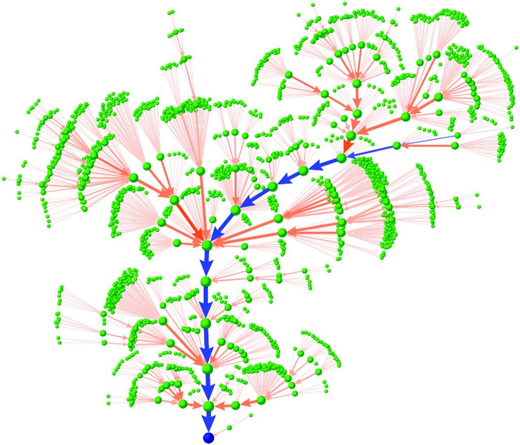
40 Boolean Networks: Mathematical Framework Figure 2.13: The Th network. The regulatory network that controls the differentiation process of T helper cells. Positive regulatory interactions are in green and negative interactions in red. The Figure is adopted from the Fig. 2 in Ref. [70]. Fibroblast signal transduction dynamics: Helikar et al. describe signal transduction in fibroblasts with a detailed Boolean network [22, 71], with 139 nodes including 59 self-couplings. This network as an interesting case because of its size and because of its large number of intertwined feedback loops of various lengths l (see also Fig. 1 in Ref. [71]). We quantify the abundance of feedback by the trace of the l-th power of the adjacency matrix A, finding tr(a) = 59, tr(a 2 )/2 = 568, tr(a 3 )/3 = and tr(a 4 )/4 = The nodes fall into two classes. There are 9 input nodes with a self-coupling. Each of these applies the identity function to its own state, not receiving signals from any other node. These nodes provide constant but choosable input to the rest of the network. Each of the remaining 130 nodes receives an input from at least one other node in this set. We call these the core nodes. The in-degree of nodes varies from 1 to 14, the out-degree varies from 1 to