Optical Fiber Intro - Part 1 Waveguide concepts

Transcription

1 Optical Fiber Intro - Part 1 Waveguide concepts Copy Right HQL Overview and study guide Loading package 1. Introduction waveguide concept 1.1 Discussion If we let a light beam freely propagates in free space, what happens to the beam?

2 2 Optical fiber intro-part 1_p.nb Plot 1 z 2, 1 z 2, z, 0,3, AspectRatio 0.05, Filling 1 2, Green The beam grows big. It can grow small like when we focus, but becomes big again after the minimum spot. This is known as diffraction. Plot 1 z 2, 1 z 2, z, 2, 4, AspectRatio 0.05, Filling 1 2, Green ParametricPlot3D z 2 Cos, z 2 Sin, z, z, 3, 8,, Pi, Pi If we like to propagate a beam while keeping it the same shape (cross section) everywhere, how do we do it? Example: A pair of parallel planar mirrors! But we don't have to use mirrors, there are other ways, the main concept is that we can engineer a medium in such a way that we can use to "guide" the beam along the desired direction of propagation, this is the concept of waveguide. Optical waveguide is simply a waveguide for light. This is to distinguish it from waveguides for other EM waves such as microwave, RF Intro to optical waveguides There are several ways to achieve optical waveguide. It is relevant, from the practical point of view, to be aware of technologies that are well established in applications vs. those that are theoretically feasible but might not be practical. Mirror or reflecting-wall optical waveguide, for example can be achieved, but are not as practical as dielectric waveguides. Holey fibers or photonic bandgap (PBG) waveguides are likewise promising for special cases but have not been as widespread as dielectric waveguides.

3 Optical fiber intro-part 1_p.nb 3 Here we'll concentrate on dielectric waveguides because this is still the principal technology in fiber optic communications Concept of total internal reflection

4 4 Optical fiber intro-part 1_p.nb Snell's law n 1 Sin 1 n 2 Sin 2 or: Sin 2 n 1 n 2 Sin 1 If n 1 n 2, there will be values of 1 such that Sin 2 1. Whent this happens, total internal reflection occurs, and the critical angle is c ArcSin n 2. n 1

5 Optical fiber intro-part 1_p.nb Waveguiding effect from total internal reflection Summary: 1- Waveguides are structures that can "conduct" light, having certain spatial profile of the optical dielectric constant 2- Because the optical dielectric constant is not spatially uniform, waveguides allow only certain optical solutions (called optical modes) that: - can be finite in space: confined or bounded modes - can extend to infinity, but only with certain relationship of the fields over the inhomogenous dielectric region 3- At the boundary between two regions of different, the boundary condition of the EM field critically determines the optical modes Ray optics concept In ray optics, the behavior light is modeled with straight lines of rays, which can be used to explain waveguide to a certain

6 6 Optical fiber intro-part 1_p.nb extent. However, only wave optics treatment is trule rigorous. Ray optics does offer a the intuitively useful concepts of acceptance angle and numerical aperture. As illustrated in the left figure, a ray enters into the perpendicular facet of a planar waveguide or fiber can be trapped (or guided) or escape into the cladding depending on the incident angle. If the incident angle is larger than certain value a, the ray will escape into the core because the condition for total internal reflection is not met. This angle is called the acceptance angle. This angle can be calculated as follow. Let c be the waveguide internal total reflection angle: c ArcSin n 2 n 1 Then, the refracted angle at the facet is: The acceptance angle is give by Snell's law: r 2 c 2 ArcSin n 2 n 1 n 0 Sin a n 1 Sin r n 0 Sin a n 1 Cos c We can approximate: n 0 Sin a n 1 1 n 2 2 n 1 2 n 1 2 n Since n 0 of air is ~ 1, we can also write: Sin a 1 2

7 Optical fiber intro-part 1_p.nb 7 What if 1 2 >1? ; ManipulatePlot x, x, 3, 0, Filling 1 2, Hue0.6, 0.4, 1,PlotRange 3, 0, 3, 3 x,, 1, 1.4, 2.5, AnimationRunning False The quantity n 0 Sin a is a measure of low large the the angular opening of the waveguide to accept (or to radiate) the beam. Thus, a concept is used to describe the quantity: numerical aperture or NA. Illustration: skew rays propagate without passing through the center axis of the fiber. The acceptance angle for skew rays is larger than the acceptance angle of meridional rays. This condition explains why skew rays outnumber meridional rays. Skew rays are often used in the calculation of light acceptance in an optical fiber. The addition of skew rays increases the amount of light capacity of a fiber. In large NA fibers, the increase may be significant. The addition of skew rays also increases the amount of loss in a fiber. Skew rays tend to propagate near the edge of the fiber core. A large portion of the number of skew rays that are trapped in the fiber core are considered to be leaky rays. Leaky rays are predicted to be totally reflected at the core-cladding boundary. However, these rays are partially refracted because of the curved nature of the fiber boundary. Mode theory is also used to describe this type of leaky ray loss. The main result of skew ray is that because it can bounce around with a larger angle (glancing blow), with the skew angle, it has a larger acceptance angle:

8 8 Optical fiber intro-part 1_p.nb n 0 Sin as n 1 Cos In other words, it increases by the term 1 Cos. 1 n 2 2 n Cos n 1 2 n Planar dielectric waveguide or slab waveguide 2.1 General concept of planar dielectric waveguide A stack of layers of dielectric materials (arbitrary number of layers) can form a waveguide as long as it has EM solutions that propagate in the plane of the layers. How do we know it functions as a waveguide? we must solve the wave equation (from the Maxwell's equations) and see if a propagating mode exists. The general wave equation is: 2 E 2 x, y, z E 0 2 (2.1a) c 2 H 2 x, y, z H 0 2 (2.1b) c In a waveguide, the dielectric is a constant along one dimension, say z. If the waveguide solution exists, then the electric field can be written: Ex, y z t, where, called the propagation constant is unknown. is the frequency of light, which is given. The wave equation becomes: 2 E 2 E x 2 y x, y E 0 (2.2) 2 c 1- If a solution of Eq. (2.2) exists, it is called a mode of the structure 2- Eq. (2.2) may have many solutions or none 3- A solution may have a unique value of, or a continuous range of value of

9 Optical fiber intro-part 1_p.nb 9 3- The mode is called a propagating wave if Re[]0 Ex. 2.1 What does the wave z t look like for: 1. =1 2. = = ; 2 ; ManipulatePlot Re z t, z, 0,50, ImageSize 600, 100, PlotRange 0, 50, 1, 1, Frame True, AspectRatio 0.1, Filling Axis, t, 0,1,, 1, 1, 2 t

10 10 Optical fiber intro-part 1_p.nb 1; 1 2 ; ManipulatePlotRe z 1t,2Re z 2t, z, 0,50, ImageSize 600, 100, PlotRange 0, 50, 1, 4, Frame True, AspectRatio 0.1, Filling Axis, t, 0,1,, 1, 1, 2, 2, 2,3 t ; 2 ; ManipulatePlot Re 1 z t, z, 0,50, ImageSize 600, 100, PlotRange 0, 50, 1, 1, Frame True, AspectRatio 0.1, Filling Axis, t, 0,1,, 0, ; 2 ; ManipulatePlot Re z t, z, 0,50, ImageSize 600, 100, PlotRange 0, 50, 1, 1, Frame True, AspectRatio 0.1, Filling Axis, t, 0,1,, 0,0.1

11 Optical fiber intro-part 1_p.nb 11 Ex. 2.2 Plot 3D the wave x2 w 2 z t for: =1 and w=2. 1; 2 ; w 2. ; AnimatePlot3D x2 w 2 Re z t, x, 10, 10, z, 0,50, ImageSize 400,400, Mesh False, PlotRange 10, 10, 0, 50, 1, 1, PlotPoints 20, 150, BoxRatios 2, 5, 1, ViewPoint 5, 8, 4, t, 0,1, AnimationRunning False Manipulate DensityPlot x2 w 2, x, 5, 5, y, 10, 10, w, 0.5,3 Manipulate Plot3D x2 w 2, x, 5, 5, y, 10, 10, PlotRange All, w, 0.5,3 Manipulate DensityPlot x2 wx 2 y2 wy 2, x, 5, 5, y, 5, 5, PlotRange All, wx,0.5,3, wy,0.5,3 Ex. 2.3 What is the wave x2 w 2 z t realtive to that of x2 w 2 z t? In other words, what does the sign of signify? 1; 2 ; w 2. ; ManipulatePlot3D x2 w 2 Re z t, x, 5, 5, z, 0,50, ImageSize 400,400, Mesh False, PlotRange 5, 5, 0, 50, 2, 2, PlotPoints 20, 150, BoxRatios 1, 5, 1, ViewPoint 5, 8, 4, t, 0,1, AnimationRunning False

12 12 Optical fiber intro-part 1_p.nb 1; 2 ; w 2. ; ManipulatePlot3D x2 w 2 Re z t, x, 5, 5, z, 0,50, ImageSize 400,400, Mesh False, PlotRange 5, 5, 0, 50, 2, 2, PlotPoints 20, 150, BoxRatios 1, 5, 1, ViewPoint 5, 8, 4, t, 0,1, AnimationRunning False 1; 2 ; w 2. ; ManipulatePlot3D x2 w 2 Re z t z t, x, 5, 5, z, 0,50, ImageSize 400,400, Mesh False, PlotRange 5, 5, 0, 50, 2, 2, PlotPoints 20, 150, BoxRatios 1, 5, 1, ViewPoint 5, 8, 4, t, 0,1, AnimationRunning False 2.2 An example: 3-layer symmetric slab waveguide In practice, for complex design, Eq. (2.2) above can be solved by numerical method. Analytical approach is useful to illustrate the qualitative aspect of the dielectric waveguide behavior. Here, we will look at the simplest 3-layer symmetric slab waveguide Consider the trivial case of symmetric 3 layers with indices 1 (cladding) and 2 (core) Solutions in each layer Equations (2.2) becomes 2 E x x E 0 (2.3) 2 c

13 Optical fiber intro-part 1_p.nb 13 which has two cases: 1- If x is in the core: 2 E x c 2 2 E 0 2- If x is in the cladding: 2 E x c 2 1 E 0 Define: k 2 1or2 2 c 2 1or2 2 (2.4.a) (2.4.b) DSolve x,x Efx k 2 2 Efx 0, Efx, x Efx c 1 sink 2 x c 2 cosk 2 x TrigToExpEfx c 1 sink 2 x c 2 cosk 2 x Efx 1 2 c 1 k 2 x 1 2 c 1 k 2 x 1 2 c 2 k 2 x 1 2 c 2 k 2 x DSolve x,x Efx k 1 2 Efx 0, Efx, x Efx c 1 sink 1 x c 2 cosk 1 x DSolve x,x Efx k 1 2 Efx 0, Efx, x Efx c 1 k 1 x c 2 k 1 x The solutions are: core;a x k 2 x ; core;b x k 2 x (2.5) in the core, where k 2 2 k (2.5a) where k c 2 and clad;a x k 1 x ; clad;b x k 1 x (2.6) for radiating wave in the cladding; k 1 1 k (2.6a) OR

14 14 Optical fiber intro-part 1_p.nb clad;a x 1 x ; clad;b x 1 x (2.7) for evanescent wave (bounded) in the cladding k 0. (2.7a) For waveguide mode (bounded), we expect only solutions Eq. (2.7) The E or H field (TE or TM): E or H Fx z t y. (2.8a) where: Fx c A A x c B B x or: Fx A x B x. c A c B (2.8b) (2.8c) Remember that we don't have to keep the term z t because it is the same everywhere Boundary condition We have the solutions k 2 x and and k 1 x or 1 x, does this mean that the problem is solved? Obviously not, because we still don't have specific solutions. These are general solutions in EACH region. They must still match each other at the boundary. For dielectric media, surface charge and surface current are zero. The boundary conditions are:. D = 0 ;. B = 0 ; (2.9) For normal component of E field: 1 E 1 2 E 2 ; (D E) (2.10) and H field: 1 H 1 2 H 2 (B H) (2.11) For most nonmagnetic media, =1, so rarely do we have discontinuity of H across an interface. For tangential E field, the component is continuous: and for zero surface current, so is the H field: E 1 E 2 (2.12) H 1 H 2 (2.13)

15 Optical fiber intro-part 1_p.nb 15 Any polarization can be split into 2 components: TE: transverse electric or TM: transverse magnetic 2.3 Boundary conditions for different polarizations TE mode Electric field is parallel to the interface: E = z t Fx y : there is only tangential component: that's why we call it transverse electric (TE) mode. What about the magnetic field? 1 c H t E x y z x y z E x E y E z x y z x y z 0 E y 0 x y z Fx 0 x Fx z t (2.14) The normal boundary condition of H (x direction) yields the same as that of E tangential boundary condition: no surprise here. The tangential boundary condition of H (z direction) yields x Fx continuity. So if we have a general solution for F[x]: c A F A B. ; (2.8c) above c B the boundary conditions, which can be written: F A B c A (2.15) F ' A ' B ' c B have to be continuous, or: A B c 1 A B A 1 ' B 1 ' A c 1 B 2 A ' 2 B ' c 2 A c 2 B. (2.16) From this, we can think of S-matrix approach again: A 2 B 2 A 2 ' B 2 ' 1 A 1 B 1 A 1 ' B 1 ' c 1 A c 1 B c 2 A c 2 B (2.17)

16 16 Optical fiber intro-part 1_p.nb or: S 11 S 12 S 21 S 22 c 1 A c 1 B c 2 A c 2 B ; (2.18) where: 2 B 2 S 11 S 12 A S 21 S 22 2 A ' 2 B ' 1 A 1 B 1 A 1 ' B 1 ' (2.19) This is called interface S-matrix. (There are several approaches to defining S matrix: do not get confused. S matrix is a generic concept, not a specific definition) TM mode In this case, the magnetic field is parallel to the interface: H = z t Fx y : we call it transverse magnetic (TM) mode. What about the electric field? 1 E c t H x y z x y z 0 Fx z t 0 c E x y z x y z Fx 0 x Fx Fx 0 x Fx z t (2.20) z t (2.21) The continuity of D normal gives F[x] continuity (but NOT electric field); the continuity of E tangential gives: 1 x Fx 1 1 x Fx F (x) derivative is discontinuous (2.22) Thus, given F F ' A B A ' B ' c A c B ; (2.15) The boundary value that we want to match is: F 1 0 A B 1 F ' 0 1 A ' B ' c A c B (2.23) To write interface S-matrix: 2 B 2 S 11 S 12 A S 21 S 22 2 A ' 2 B ' A A 1 ' B 1 B 1 ' = 2 2 A B A 2 ' B 2 ' A B 1 A 1 ' B 1 ' (2.24)

17 Optical fiber intro-part 1_p.nb Equations for solutions The solution is obtained by satisfying all boundary conditions. Each boundary condition gives a set of equation. Various coefficients will be determined by the Eqs. 2.4 Bounded mode TE Characteristic equation The S matrix for the core: FullSimplify k 2 xl k 2 xl k 2 k 2 xl k 2 k 2 xl.inverse k 2 x k 2 x k 2 k 2 x k 2 k 2 x coslk 2 sinlk 2 k 2 sinlk 2 k 2 coslk 2 Notice that the S matrix has translational symmetry. This connect the left and the right of the core region: S 2 coslk 2 sinlk 2 k 2 sinlk 2 k 2 coslk 2 For TE mode, the interface M matrix is unity. The eigen equation is: right most right A x 1 most B x 1 right x most right A x 1 x most B x 1 Here is a way to choose neat solution:. c An c Bn left most left A x 1 most B x 1 S Total left x most left A x 1 x most B x 1. c A1 c B1

18 18 Optical fiber intro-part 1_p.nb A right most x 1 xl ; B right most x 1 xl A left most x 1 x ; B left most x 1 x c right coslk 2 sinlk 2 k 2 sinlk 2 k 2 coslk c left 0 0 FullSimplifyInverse 1 1. c right 1 1 coslk 2 sinlk 2 k 2 sinlk 2 k 2 coslk c left c right c left coslk 2 sinlk k k 2 1 sinlk 2 c left k k 2 1 There are 2 equations. For the first one, the only way we have a non-trivial solution is: coslk 2 sinlk k k This is the characteristic equation: it says that we can't just choose arbitrary value of to satify the wave equation. There is a unique propagation constant for each mode. What does the second equation give us? c right c left sinlk 2 k k 2 1 a proportional relation between c right and c left : we can choose an arbitrary c left, then c right is fixed or vice versa. The wave amplitude is fixed relatively between sections, there is ONLY ONE arbitrary amplitude for the whole wave, as it should be. There are several way to express the same characteristic equation: CosLk 2 SinLk 2 k k 2 1 cotlk 2 k k 2 1

19 Optical fiber intro-part 1_p.nb 19 coslk 2 sinlk k L 2 a 2 k 2 1 cos2 ak 2 sin2 ak k k TrigExpandcos2 ak 2 sin2 ak k k 2 1 cos 2 ak 2 sina k 2 1 cosa k 2 k 2 sina k 2 k 2 cosa k 2 1 sin 2 ak 2 Factor cosa k 2 1 sina k 2 k 2 cosak 2 k 2 sina k 2 1 k 2 1 cosak 2 1 sinak 2 k 2 cosak 2 k 2 sinak We notice that this means this single characteristic equation gives us 2 separate characteristic sub-equations: cosak 2 1 sinak 2 k 2 0 AND cosak 2 k 2 sinak What is the meaning of this? It means that there are two classes of modes and solutions, one for each equation. But why? because of symmetry: in any quantum problem, if we have symmetry, we have a subset of eigensolutions that belong to an eigenspace of that geometry. Similarly here, we have a symmetric waveguide, which has the reflection symmetry that have even solution: F[x]=F[-x] or odd solution F[x]=-F[-x]: We can guess that each "sub-characteristic" equation is for each class of modes and solutions. If fact, the even solutions are: Cosk 2 x in the core. At the core boundary: Cosk 2 a k 2 Sink 2 a. In the cladding, the solution is C 1 xa : At the cladding boundary: Cosk 2 a Cosk 2 a the equation is: k 2 Sink 2 a Cosk 2 a 1 C C 1. Choose C Cosk 2 a, Obviously, the charac. eq. is: k 2 Sink 2 a Cosk 2 a 1 or Cosk 2 a 1 k 2 Sink 2 a 0. We can similarly verify the same for odd solutions.

20 20 Optical fiber intro-part 1_p.nb ResolvTEnindex_List, a_, _, neff_ : Module1, 2, 1, k2, k0, 1, 2 nindex^2 ; k0 2 Pi ; 1 k0 SqrtAbsneff ^2 1;k2k0 SqrtAbs2 neff ^2; cosa k2 1 sina k2 k2cosa k2 k2 sina k2 1 ; indexprof 3.4, 3.5 ; a 2.5 ; 1.5 ; PlotResolvTEindexprof, a,, x, x, 3.4, The roots of the equation are where the function crosses the horizontal axis, which is ==0. These are discrete modes of the waveguide. FindRootResolvTE3.4, 3.5, 2.5,1.5,n 0, n, 3.42, 3.44 n This value n (example is above) is called the MODE EFFECTIVE INDEX. n eff k 0 In other words, the mode acts as if it sees this index value in the waveguide. 2- Each mode has its own index, different from each other 3- The speed of propagation is: v c, hence different modes move at different speeds. n eff This causes INTERMODAL DISPERSION. If a light pulse is a linear combination of many modes, each modal component will move at its own speed, and after awhile, be out of step with others EM field So we find the mode. How do we find the E field? Fx 1 xa 1 xa Left region: x Fx 1 1 xa 1 1 xa. c left 0

21 Optical fiber intro-part 1_p.nb 21 Middle or core region: k 2 x k 2 x k 2 k 2 x k 2 k 2 x. c m1 c m2 Inverse Fx x Fx k 2 x k 2 x k 2 k 2 x k 2 k 2 x. c m1 c m2 c m1 c m2 xa 1 xa 1 xa 1 1 xa 1 1 xa. c left 0 k 2 x k 2 x k 2 k 2 x k 2 k 2 x xa. 1 xa 1 xa xa 1 1 xa 1 1 xa xa. 0 c left Remember interface S matrix? S= k 2 x n k 2 x n k 2 k 2 x n k 2 k 2 x n 1. 1 x n 1 1 x n 1 x n 1 1 x n So here is how to get the full solution: Chose c left 1 (or anything we like, except for 0) Use S interface matrix to get to the next region, and the next, and so on... But: use the "second" equation to get the last region. z t Finally: E=F[x] c H x y z H x H z 1 k 0 Fx x Fx Fx 0 x Fx z t z t FullSimplifyInverse k 2 x k 2 x k 2 k 2 x k 2. 1 xa 1 xa k 2 x 1 1 xa 1 1 xa. x a ak 2 k 2 1 ak 2 k2 1 2 k 2 2 k 2 ak 2 k 2 1 ak 2 k2 1 2 k 2 2 k 2 ak 2 k 2 1 ak 2 k2 1 2 k 2 2 k 2 ak 2 k 2 1 ak 2 k2 1 2 k 2 2 k ak 2 k k 2 ak 2 k k 2

22 22 Optical fiber intro-part 1_p.nb FullSimplify k 2 x k 2 x k 2 k 2 x k 2 k 2 x. ak 2 k k 2 ak 2 k k 2 cosa x k 2 sinax k 2 1 k 2 cosa x k 2 1 sina x k 2 k 2 So the solutions are: IfAbsx a, in the core region Left side: (x<0): cosa x k2 sinax k2 1 k2 1 xa this is Ey, 1 1 xa k0 this is Hz, neff 1 xa this is Hx this is Ey, cosa x k2 1 sina x k2 k2k0 this is Hz sinax k2 1, neff cosa x k2 this is Hx k2 Right side: x>0 1 xa Sign sin2 a k2 this is Ey, 1 1 xa k0 this is Hz, neff 1 xa this is Hx For practical use, we still need to normalize: a sina x k2 1 FullSimplifyCoreintegration cosa x k2 a k2 2 x 2k2cos4 a k a k k2 1k2 1 sin4 a k2 4k2 3 FullSimplifyCladintegration a 1 xa 2 x If a 0 Re1 0, 1 2 1, a 2 xa 1 x

23 Optical fiber intro-part 1_p.nb 23 N factor: cos4 a k2 112 a k k21k21 sin4 a k2 2k2 2 4k FieldTEnindex_List, a_, _, neff_, x_ : Module1, 2, 1, k2, k0, Norm, 1, 2 nindex^2 ; k0 2 Pi ; 1 k0 SqrtAbsneff ^2 1;k2k0 SqrtAbs2 neff ^2; Norm cos4 a k2 1 12ak k2 2 k2 1k2 1sin4 a k2 1 4k2 3 1 ; 1 IfAbsx a, Norm sina x k2 1 cosa x k2 this is Ey k2, cosa x k2 1 sina x k2 k2k0 this is Hz sina x k2 1, neff cosa x k2 this is Hx k2 1 xa,ifx0, this is Ey,, 1 1 xa k0 this is Hz, neff 1 xa this is Hx sin2 a k2 k k21 1 xa this is Ey, 1 1 xa k0 this is Hz, neff 1 xa this is Hx ;

24 24 Optical fiber intro-part 1_p.nb ParmTEnindex_List, a_, _, neff_ : Module1, 2, 1, k2, k0, Norm, 1, 2 nindex^2 ; k0 2 Pi ; 1 k0 SqrtAbsneff ^2 1;k2k0 SqrtAbs2 neff ^2; Norm cos4 a k2 1 12ak k2 2 k2 1k2 1sin4 a k2 1 4k2 3 1 ; a, neff,1, k2, k0, Norm ; FieldTE2parm_List, x_ : Modulea, neff,1, k2, k0, Norm, a, neff,1, k2, k0, Norm parm ; 1 IfAbsx a, Norm sina x k2 1 cosa x k2 this is Ey k2, cosa x k2 1 sina x k2 k2k0 this is Hz sina x k2 1, neff cosa x k2 this is Hx k2 1 xa,ifx0, this is Ey,, 1 1 xa k0 this is Hz, neff 1 xa this is Hx sin2 a k2 k k21 1 xa this is Ey, 1 1 xa k0 this is Hz, neff 1 xa this is Hx ; Illustration: what does the "profile" looks like We can plot F[x] which is directly proportional to Ey profile for various mode

25 Optical fiber intro-part 1_p.nb 25 nindex 3.4, 3.5; a 2.5 ; 1.5 ; PlotResolvTEnindex, a,, x, x, nindex1, nindex nindex 3.4, 3.5; a 2.5 ; 1.5 ; segment 3.499, 3.495, 3.48, 3.47, 3.45, 3.42, 3.405; neff ; For i 1, i 7, i, AppendToneff, x. FindRootResolvTEnindex, a,, x 0, x, segmenti 1, segmenti neff , , , , ,

26 26 Optical fiber intro-part 1_p.nb allp ; nindex 3.4, 3.5; a 2.5 ; 1.5 ; Fori 1, i Lengthneff 1, i, parm ParmTEnindex, a,, neffi ; AppendToallp, PlotFieldTE2parm, x1, x, 7, 7,PlotRange 1., 1, PlotStyle Thickness0.02, Huei 0.1, 1, 0.8, Filling 1 Axis, Huei 0.1, 1, 0.8, 0.5,Ticks None, AspectRatio 1. ; ShowGraphicsRowallp Traveling electric field The field is essentially a standing wave in the x direction (because of waveguide) and a traveling wave in the z direction Link to imode 1; 2 neffimode ; 2 ; parm ParmTEnindex, a,, neffimode ; allp ; Fori 1, i 40, i, t i ; PrintTemporary"i ", i; AppendToallp, Plot3DFieldTE2parm, x1 Cos z t, x, 4, 4, z, 0,2, ImageSize 400, 200, PlotPoints 15, 40, Mesh False, PlotRange 4, 4, 0, 2, 1, 1, BoxRatios 4, 2, 1, ViewPoint 5, 8, 6 ; Animateallpi, i, 1, Lengthallp, 1, AnimationRunning False Link to Fig Vector graphics Remember that EM field are vector field. Not scalar field. We can look at the amplitude of a single component, but to have

27 Optical fiber intro-part 1_p.nb 27 a sense of what really happens, we must look at vector field. Linked to Fig Magnetic field lines of mode 0 What does the Hz component look like (compared with Hy?) PlotFieldTEnindex, a,, neff1, x1,imfieldtenindex, a,, neff1, x 2, FieldTEnindex, a,, neff1, x3, x, 7, 7,PlotRange All, PlotStyle Hue0, 1, 0.8, Hue0.4, 1, 0.8, Hue0.8, 1, The vector field varies smoothly at the center and "turns" at the boundary Link to Fig Link to Where we have interference with higher kx, we see "twirl" or vortex, or whirpool: this is in higher order mode Linked to Fig Linked to Fig Field lines Field line is a concept that "draws" the line that a vector field tries to follow. If we have a line {x[s],y[s],z[s]}. Then its tangential vector is: s xs, s ys, s zs F x, F y, F z where is just a proportional constant, which can be 1. Thus, the system of D. E. is: s xs ys zs F x xs, ys, zs F y xs, ys, zs F z xs, ys, zs analytically. For example in this case:. It is quite simple to integrate this eq. numerically. In simple case, we can even do it

28 28 Optical fiber intro-part 1_p.nb s xs ys zs Re Cosk x 0 k Sink x z Cosk x Sin z 0 k Sink x Cos z TrigReduce Cosk xs Sin zs k Sink xs Cos zs sink xs zs sink xs zs k sink xs zs k sink xs zs k xs zs kxs zs k k. x z FullSimplify k k Sinus Sinvs k Sinvs k Sinus k sinvs k sinus s us vs sinvs sinus u' Sin[u]+v' Sin[v]==0 s Cosu Cosv 0 Cos[u]+Cos[v]= Constant

29 Optical fiber intro-part 1_p.nb 29 k 0.25; 1.; fl ; Fori 1, i 21, i, AppendTofl, ContourPlotCosk xycosk xy i , y, 10, 10, x, 10, 10, PlotPoints 100, ContourStyle Huei 0.045, 1, 0.9, Thickness0.005, DisplayFunction Identity Showfl, DisplayFunction $DisplayFunction Link to section Profile of all components: Ey, Hx, and Hz Link to section fig a 2.5 Bounded mode TM Characteristic equation The S matrix for the core: S 2 coslk 2 sinlk 2 k 2 sinlk 2 k 2 coslk 2 For TE mode, the interface M matrix is unity. The eigen equation is: c An c Bn right most right A x 1 most B x 1 M.. right x most right A x 1 x most B x 1 left most left A x 1 most B x 1 S Total.M. left x most left A x 1 x most B x 1 Here is a way to choose neat solution:. c A1 c B1

30 30 Optical fiber intro-part 1_p.nb A right most x 1 xl ; B right most x 1 xl A left most x 1 x ; B left most x 1 x c right coslk 2 sinlk 2 k 2 sinlk 2 k 2 coslk c left 0 0 c right FullSimplifyInverse coslk 2 sinlk 2 k 2 sinlk 2 k 2 coslk c left c right c left coslk 2 sinlk k 2 1 sinlk 2 k sinlk 2 c left k k There are 2 equations. For the first one, the only way we have a non-trivial solution is: coslk 2 sinlk k 2 1 k This is the characteristic equation: it says that we can't just choose arbitrary value of. There is a unique propagation constant for each mode. What does the second equation give us? c right c left sinlk 2 k k Similar as above, we can decompose the characteristic equation TrigExpandcosLk 2 sinlk k 2 1 k L 2 a cos 2 ak 2 sina k cosa k 2 k 2 1 sina k 2 k 2 1 cosa k sin 2 ak 2 Factor cosa k sina k 2 k 2 1 cosa k 2 k 2 1 sina k k

31 Optical fiber intro-part 1_p.nb 31 ResolvTMnindex_List, a_, _, neff_ : Module1, 2, 1, k2, k0, 1, 2 nindex^2 ; k0 2 Pi ; 1 k0 SqrtAbsneff ^2 1; k2 k0 SqrtAbs2 neff ^2; cosa k2 2 1 sina k2 k2 1cosa k2 k2 1 sina k2 2 1 ; nindex 3.4, 3.5 ; a 2.5 ; 1.5 ; PlotResolvTMnindex, a,, x, x, 3.4, FindRootResolvTM3.4, 3.5, 2.5,1.5,x 0, x, 3.405,3.42 x EM field How do we find the EM field? H = z t Fx y c E x y z Fx 0 x Fx z t Left region: Fx x Fx Middle or core region: M 2. k 2 x k 2 x 1 xa 1 xa 1 1 xa 1 1 xa. Fx x Fx k 2 k 2 x k 2 k 2 x. k 2 x k 2 x c left 0 k 2 k 2 x k 2 k 2 x. c m1 c m2 xa M 1. 1 xa c m1 c m2 1 xa 1 1 xa 1 1 xa. c left 0 xa

32 32 Optical fiber intro-part 1_p.nb c m1 c m2 Inverse k 2 x k 2 x k 2 k 2 x k 2 k 2 x xa.m T. 1 xa 1 xa 1 1 xa 1 1 xa xa. 0 c left Remember interface S matrix? S= k 2 x n k 2 x n k 2 k 2 x n k 2 k 2 x n 1.M T. 1 x n 1 1 x n 1 x n 1 1 x n So here is how to get the full solution: Chose c left 1 (or anything we like, except for 0) Use S interface matrix to get to the next region, and the next, and so on... But: use the "second" equation to get the last region. Again: H = z t Fx y c E x y z E x E z 1 k 0 Fx x Fx Fx 0 x Fx z t z t FullSimplifyInverse k 2 x k 2 x k 2 k 2 x k 2 k 2 x xa 1 xa 1 1 xa 1 1 xa. x a ak 2 k ak 2 k k k 2 1 ak 2 k ak 2 k k k 2 1 ak 2 k ak 2 k k k 2 1 ak 2 k ak 2 k k k ak 2 k k 2 1 ak 2 k k 2 1

33 Optical fiber intro-part 1_p.nb 33 FullSimplify k 2 x k 2 x k 2 k 2 x k 2 k 2 x. ak 2 k k 2 1 ak 2 k k 2 1 cosa x k 2 sinax k k 2 1 cosax k sina x k 2 k 2 Normalization of Ex a sina x k2 2 1 FullSimplifyCoreintegration cosa x k2 a k2 1 2 x 1 4k k cos4 a k2 1 2 a k k k sin4 a k2 neff cos4ak2 12 a k k k2 12 1k sin4 a k2 4k FullSimplifyCladintegration a 1 xa 2 x If a 0 Re1 0, 1 2 1, a 2 xa 1 x

34 34 Optical fiber intro-part 1_p.nb FieldTMnindex_List, a_, _, neff_, x_ : Module1, 2, 1, k2, k0, Norm, 1, 2 nindex^2 ; k0 2 Pi ; 1 k0 SqrtAbsneff^2 1 ; k2 k0 SqrtAbs2 neff^2 ; Norm neff Cos4 ak2 1 2ak k k k Sin4 ak2 4k neff ; Sina x k2 2 1 IfAbsx a, Cosa x k2 k2 1, Cosa x k2 2 1 Sina x k2 k2 1 Sina x k2 2 1,neff Cosa x k2 k2 1 1 xa, If x 0,, 1 1 xa 1k0, neff 1 xa 1, Sin2 ak2 k k xa, 1 1 xa 1k0, neff 1 xa 1 2 k0 2

35 Optical fiber intro-part 1_p.nb 35 ParmTMnindex_List, a_, _, neff_ : Module1, 2, 1, k2, k0, Norm, Norm 1, 2 nindex^2 ; k0 2 Pi ; 1 k0 SqrtAbsneff ^2 1 ;k2 k0 SqrtAbs2 neff ^2; neff cos4 a k2 1 2 a k k k2 1 21k2 1 21sin4 a k2 4k neff ; a, 1, 2, neff, 1, k2, k0, Norm ; FieldTM2parm_List, x_ : Modulea, 1, 2, neff, 1, k2, k0, Norm, 1 Norm a, 1, 2, neff, 1, k2, k0, Norm parm ; IfAbsx a, sina x k2 2 1 cosa x k2 k2 1 cosa x k2 2 1, 1 sina x k2 k2 2k0,neff sina x k2 2 1 cosa x k2 k xa,ifx0,, 1 1 xa 1k0,neff 1 xa 1 sin2 a k2 k , 2k xa, 1 1 xa 1k0,neff 1 xa 1 ;

36 36 Optical fiber intro-part 1_p.nb nindex 1, 3.5; a 0.5 ; 1.5 ; PlotResolvTMnindex, a,, x, x, nindex1, nindex The most important feature of TM mode: the E field discontinuity What does the trasnverse magnetic field Hy look like? Linked to Fig But remember the normal electric field Ex boundary condition: 1 E x;1 2 E x;2 Linked to Fig An important concept (for all waveguide, not just slab): confinement factor: How much of the electric field is really in the core region? We'll see about this in later section. F[x] is directly proportional to Hy profile for various mode

37 Optical fiber intro-part 1_p.nb 37 nindex 1, 3.5; a 0.5 ; 1.5 ; PlotResolvTMnindex, a,, x, x, nindex1, nindex segment2 3.49,3.4,3,2.5,1.5,1.01; neff ; For i 1, i Lengthsegment2, i, AppendToneff, x. FindRootResolvTMnindex, a,, x 0, x, segment2i 1, segment2i neff , , , , Let's look at the transverse magnetic Hy

38 38 Optical fiber intro-part 1_p.nb allp ; Fori 1, i Lengthneff, i, parm ParmTMnindex, a,, neffi ; AppendToallp, PlotFieldTM2parm, x1, x, 2, 2,PlotRange 10., 10, PlotStyle Thickness0.02, Huei 0.1, 1, 0.8, Filling 1 Axis, Huei 0.1, 1, 0.8, 0.5,Ticks None, AspectRatio 0.75 ; ShowGraphicsRowallp Let's look at the Electric field Ex allp ; Fori 1, i Lengthneff, i, parm ParmTMnindex, a,, neffi ; AppendToallp, PlotFieldTM2parm, x3, x, 2, 2,PlotRange 2., 2, PlotStyle Thickness0.012, Huei 0.1, 1, 0.8, Filling 1 Axis, Huei 0.1, 1, 0.8, 0.5,Ticks None, AspectRatio 0.75 ; ShowGraphicsRowallp Fig Compare Hy and Ex of the lowest order mode:

39 Optical fiber intro-part 1_p.nb 39 PlotReFieldTMnindex, a,, neff1, x1, 2 ReFieldTMnindex, a,, neff1, x3, x, 1, 1,PlotStyle RGBColor1., 0., 0, RGBColor0., 0., Compare Hy and Ex of the highest order mode: PlotReFieldTMnindex, a,, neff5, x1, 2 ReFieldTMnindex, a,, neff5, x3, x, 4, 4,PlotRange 4, 4, All,PlotStyle RGBColor1., 0., 0, RGBColor0., 0., 1,AspectRatio Linked to reviewed materials 3. Key concepts of waveguide

40 40 Optical fiber intro-part 1_p.nb Although we study a particular waveguide geometry above, the slab waveguide, several important concepts are applicable to any waveguide, and can be illustrated with the slab waveguide. 3.1 Intensity and energy flow Energy flow: Poynting vector - TE mode Intensity inside a waveguide is obtained by evaluating the Poynting vector. The time-averaged Poynting vector is: S c Re 8 E H (3.1) Consider the example of slab waveguide. For TE mode: E = Ex, z y t (3.2) x y z H E x y z (3.3) k 0 0 E y 0 k 0 x y z z E y x, z 0 x E y x, z t S c Re 8 E H c 8 1 k 0 Re x y z 0 E y 0 z E y x, z 0 x E y x, z (3.4) Det x y z 0 Ef y x, z 0 z Ef y x, z 0 x Ef y x, z z Ef y x, zef y 0,1 x, z x Ef y x, zef y 1,0 x, z S c8 Re E H c Re x E y x, z E y 8 k 0 x z E y x, z E y z (3.5) Is it possible for a net energy to flow along x direction? Intuitively, no. The energy can bounce back and forth from within the waveguide, but the net roundtrip (or the total space average) must be zero. If E y x, z is real, then so is E y and Re x E y x, z E y 0: Obviously the intensity along x direction = 0. But the x x

41 Optical fiber intro-part 1_p.nb 41 principle must be true much more generally, not for just this case of TE mode and real E y x, z. The intensity of the z-traveling component is given by: S.z c Re E y x, z E y 8 k 0 (3.6) and the power is given by: P S.z x z c 8 k Re E y x, z E y x (3.7) 0 z For mode m: E y z m m z E m x (3.8) The intensity is: S.z c 8 k 0 m E m x ^2 (3.9) cn eff;m 8 E m x ^2 P cn eff;m 8 E m x 2 x (3.10) These expressions are very similar to planewave, with the difference being the effective index, which is mode-dependent. This is the reason why normalization with respect to power is slightly different from normalization with respect to wavefunction: For just wavefunction: E m x ^2 1. (3.11a) For power: n eff;m E m x ^2 x 1 (3.11b) (all other constants are dropped for convenient). Either way is fine as long as one remembers what to use in each calculation For TM mode S c 8 1 k 0 Re x H y H y 1,0 x, z z Hy H y 0,1 x, z (3.12) The intensity is given by: S.z c Re H y x, z H y (3.13) 8 k 0 z Now we need to convert to Ex: For a given mode m: E x z H y x, z. (3.14) k 0 E m;x m H y x, z k 0 m H y x, z n eff;m H y x, z k 0 (3.15)

42 42 Optical fiber intro-part 1_p.nb Thus: H y x, z n eff;m E m;x. (3.16) Then: S.z c 8 n eff;m Re E m;x E m;x (3.17) c 8 n eff;m E m;x 2 Indeed that the intensity for TM mode is proportional to the transverse component of the electric field, as expected. The power of the mth mode is given by: P m S m.z x c 8 n eff;m x E m;x 2 x (3.18) Notice that x E m;x 2 x can be written as: x E m;x 2 x xem;x 2 x E m;x 2 x E m;x 2 x E m;x 2 x (3.19) where is the spatial average of. Thus: P m c 8 n eff;m E m;x 2 x. (3.20) Notice the suttle difference in the power expression of TE and TM mode. The ratio average index. n eff;m can be considered as a modal 3.1.3: In the lab: intensity plot In the lab, if we look at a waveguide facet, what to we see? We see the intensity. nindex 3.4, 3.5; a 2.5 ; 1.5 ; segment 3.499, 3.495, 3.48, 3.47, 3.45, 3.42, 3.405; neffte ; For i 1, i Lengthsegment, i, AppendToneffTE, x. FindRootResolvTEnindex, a,, x 0, x, segmenti 1, segmenti ; alldpte ; Fori 1, i LengthneffTE 1, i, AppendToalldpTE, DensityPlotneffTEi AbsFieldTEnindex, a,, nefftei, x1^2, y, 0,20, x, 4, 4, PlotPoints 2, 202, Mesh False, ColorFunction GrayLevel,ImageSize 700, 200, AspectRatio 2 7.

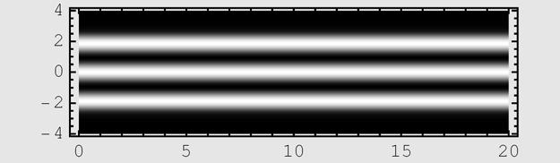
43 Optical fiber intro-part 1_p.nb 43 alldpte Intensity plot,,,,,

44 44 Optical fiber intro-part 1_p.nb We recall earlier that for some TM mode, if the index difference is large, the E field leakage is also quite large. We can see how it is in this example. Note: this waveguide is NOT the same as what we show for TE above. nindex 1, 3.5; a 0.5 ; 1.5 ; PlotResolvTMnindex, a,, x, x, nindex1, nindex

45 Optical fiber intro-part 1_p.nb 45 segment2 3.49,3.4,3,2.5,1.5,1.01; nefftm ; For i 1, i Lengthsegment2, i, AppendToneffTM, x. FindRootResolvTMnindex, a,, x 0, x, segment2i 1, segment2i ; alldptm ; Epsx_ : IfAbsx a, nindex2^2, nindex1^2; Fori 1, i LengthneffTM, i, PrintTemporaryi; AppendToalldpTM, DensityPlotEpsxneffTMi AbsFieldTMnindex, a,, nefftmi, x3^2, y, 0,20, x, 1.5, 1.5, PlotPoints 2, 200, ColorFunction GrayLevel,ImageSize 700, 200, AspectRatio 2 7. alldptm TM mode intensity: note the discontinuity

46 46 Optical fiber intro-part 1_p.nb,,,,

47 Optical fiber intro-part 1_p.nb Confinement factor An important concept (for all waveguide, not just slab): confinement factor: How much of the electric field is really in the core region? The fraction of the field in the core is called the confinement factor. (in complex structure, we need to define what "core" region is the region of our interest) core Ex,y 2 x y Ex,y 2 x y (3.21) all 3.3 Multi-mode propagation Concept If we launch an optical beam into a multimode waveguide, what do we get out at the other end? Again we apply the principle of linear superposition: N x m1 a m F m x. (3.22) We can represent the input signal as a finite-rank vector: a 1 a 2. a N. The full expression of the electric field is: N E m1 a m E m x m z t t N m1 a m E m x m z (3.23) We notice one very important feature: we cannot separate the x and z dependent component of the net field E anymore. Thus: while the z-dependent and the x-dependent component can be separated for every eigenmode of the waveguide, they can not be so for any arbitrary wave. The reason is modal dispersion as discussed above: each mode has a different propagation constant m. What does this entail? Remember how when you add waves together, not only amplitude but also phase is very important? Let's consider the input signal at z=0: At z=l, we have: Ex, z 0 t N m1 a m E m x. (3.24) Ex, z L t N m1 a m m L E m x t N m1 a m ' E m x (3.25) where a m ' a m m L. Thus, the profile Ex, z L can be very different from that at z=0. This very important aspect is the foundation for waveguide circuit: modulate and control of light path through waveguide Example Consider a slab waveguide with 2 modes:

48 48 Optical fiber intro-part 1_p.nb nindex 1.4, 1.5; a 1.25 ; 1.5 ; PlotResolvTEnindex, a,, x, x, nindex1, nindex segment 1.49, 1.46, 1.42; neff ; For i 1, i Lengthsegment, i, AppendToneff, x. FindRootResolvTEnindex, a,, x 0, x, segmenti 1, segmenti neff , Let's look at the waveguide mode

49 Optical fiber intro-part 1_p.nb 49 PlotFieldTEnindex, a,, neff1, x1,fieldtenindex, a,, neff2, x1, x, 6, 6,PlotRange 1., 1, PlotStyle Thickness0.01, Hue0.35, 1, 0.5, Thickness0.01, Hue0.8, 1, At z=0, let's have a wave that consists of half and half of the low mode and the high mode: w 0.5; Plotw FieldTEnindex, a,, neff1, x1 1 w FieldTEnindex, a,, neff2, x1, x, 4, 4,PlotRange 1., 1, PlotStyle Thickness0.01, Hue0.35, 1, 0.5, Thickness0.01, Hue0.8, 1, What does this wave look like as it propagates along the waveguide? At z= 0: Ex, z t E 1 x E 2 x Ex, z L 1 2 t 1 L E 1 x 2 L E 2 x

50 50 Optical fiber intro-part 1_p.nb 1 2 t 1 L E 1 x 2 1 L E 2 x What happens at z=l when 2 1 L? Ex, z L 1 2 t 1 L E 1 x E 2 x Let's compare the field profile at z=0 and z=l, dropping the oscilling term t 1 L : w 0.5; Plotw FieldTEnindex, a,, neff1, x1 1 w FieldTEnindex, a,, neff2, x1, w FieldTEnindex, a,, neff1, x1 1 w FieldTEnindex, a,, neff2, x1, x, 4, 4,PlotRange 1., 1, PlotStyle Thickness0.01, Hue0.35, 1, 0.5, Thickness0.01, Hue0.8, 1, Remarkable: this tells us that the profile changes quite a bit as the wave propagates: it is not always a constant profile wave in a waveguide! What if it keeps on going? Ex, z 2 L 1 2 t 2 1 L E 1 x L E 2 x and 2 1 L : Ex, z 2 L 1 2 t 2 1 L E 1 x E 2 x: we are back to square one again. We can see all this by looking at its intensity. From the above expression of the Poynting vector: S.z c Re E y x, z E y 8 k 0 z E y x, z we y;1 x 1 z 1 w E y;2 x 2 z E y z 1 we y;1 x 1 z 2 1 w E y;2 x 2 z E y x, z E y we y;1 x 1 z 1 w E y;2 x 2 z z 1 we y;1 x 1 z 2 1 w E y;2 x 2 z w.;

51 Optical fiber intro-part 1_p.nb 51 Expandw Ef y;1 x 1 z u Ef y;2 x 2 z 1 w Ef y;1 x 1 z 2 u Ef y;2 x 2 z E y x, z E y w 2 1 Ef 1 x 2 u 2 2 Ef 2 x 2 z z z uwef 2 x Ef 1 x There is a real term: w 2 1 Ef 1 x 2 u 2 2 Ef 2 x 2 which is the individual sum of the intensity of each component. But more importantly, there is the interference term: z z uwef 2 x Ef 1 x. What is the effect of this interference term? Let's plot it out: w 0.5; 2 neff; Plot3DRew FieldTEnindex, a,, neff1, x1 1 z 1 w FieldTEnindex, a,, neff2, x1 2 z 1 z w 1 FieldTEnindex, a,, neff1, x1 1 w 2 FieldTEnindex, a,, neff2, x1 2 z, z, 0,30, x, 2.5, 2.5, PlotPoints 120, 40,PlotRange All, Mesh False, BoxRatios 30, 5, 5, ViewPoint 0, 0, 5 Notice what happens: the wave seems to move from right side of the waveguide to left and back to right again and so on... : this is the behavior of a ray that bounces back and forth between the two boundary surface. Where is the shift maximum?

52 52 Optical fiber intro-part 1_p.nb L Abs What is a coupler? why is it called? We have a waveguide with this property: cladding index= 1.4 ; thickness 2.5 um, the core index can be tuned with an external electric field from 1.43 to 1.5. A beam with 1.5 um wavelength is coupled to one side of the waveguide (mode1 + mode2), how does the external electric field can change its propagation property? nindex 1.4, ncore; a 1.25 ; 1.5 ; allp ; Fori 1, i 12, i, ncore 1.45 i ; AppendToallp, PlotResolvTE1.4, ncore, a,, x, x, 1.4,ncore, DisplayFunction Identity Showallp, DisplayFunction $DisplayFunction Graphics

53 Optical fiber intro-part 1_p.nb 53 nindex 1.4, 1.45; a 1.25 ; 1.5 ; PlotResolvTEnindex, a,, x, x, nindex1, nindex Graphics segment 1.44, 1.43, 1.401; neff ; For i 1, i Lengthsegment, i, AppendToneff, x. FindRootResolvTEnindex, a,, x 0, x, segmenti 1, segmenti neff ,

54 54 Optical fiber intro-part 1_p.nb w 0.5; 2 neff; plot1 Plot3DRew FieldTEnindex, a,, neff1, x1 1 z 1 w FieldTEnindex, a,, neff2, x1 2 z 1 z w 1 FieldTEnindex, a,, neff1, x1 1 w 2 FieldTEnindex, a,, neff2, x1 2 z, z, 0,30, x, 2.5, 2.5, PlotPoints 120, 40,PlotRange All, Mesh False, BoxRatios 30, 5, 5, ViewPoint 0, 0, 5 nindex 1.4, 1.55; a 1.25 ; 1.5 ; PlotResolvTEnindex, a,, x, x, nindex1, nindex2 segment 1.54, 1.5, 1.46; neff ; For i 1, i Lengthsegment, i, AppendToneff, x. FindRootResolvTEnindex, a,, x 0, x, segmenti 1, segmenti neff ,

55 Optical fiber intro-part 1_p.nb 55 w 0.5; 2 neff; plot2 Plot3DRew FieldTEnindex, a,, neff1, x1 1 z 1 w FieldTEnindex, a,, neff2, x1 2 z 1 z w 1 FieldTEnindex, a,, neff1, x1 1 w 2 FieldTEnindex, a,, neff2, x1 2 z, z, 0,30, x, 2.5, 2.5, PlotPoints 120, 40,PlotRange All, Mesh False, BoxRatios 30, 5, 5, ViewPoint 0, 0, SurfaceGraphics 3.4 Modal dispersion How does the depend on?

56 56 Optical fiber intro-part 1_p.nb nindex 1.4, 1.5; a 1.25 ; c ; plot1 Plot3DResolvTEnindex, a, c f, x, x, nindex , nindex , f,2,4., PlotPoints 70, 30, DisplayFunction Identity ; plot2 Plot3D0, x, nindex , nindex , f,2,4., PlotPoints 2, DisplayFunction Identity ; Showplot1, plot2, DisplayFunction $DisplayFunction, ImageSize 500, 500, BoxRatios 1, 1, 1, ViewPoint 2, 5, 3 Linked to Fig Graphics3D Plots of [] or n eff or [f] or n eff f or [] or n eff as a function of frequency are called dispersion curves.

57 Optical fiber intro-part 1_p.nb 57 nindex 1.4, 1.5; a 1.25 ; c ; plot1 Plot3DResolvTEnindex, a,, x, x, nindex , nindex ,, 0.75,1.5, PlotPoints 70, 30, DisplayFunction Identity ; plot2 Plot3D0, x, nindex2, nindex1,, 0.75,1.5, PlotPoints 2, DisplayFunction Identity ; Showplot1, plot2, DisplayFunction $DisplayFunction, ImageSize 500, 500, BoxRatios 1, 1, 1, ViewPoint 2, 5, 3 We would expect that 2 n eff n eff c c where is some sort of averaged dielectric constant of the waveguide, because n eff is approximately the modal average of the entire dielectric constant profile: n eff;m xe mx 2 x Em x 2 x However, as the frequency change, the mode profile changes, and n eff is not constant for each mode. Recalling what we define as dispersion:

58 58 Optical fiber intro-part 1_p.nb n eff InverseGVDterm c ; n eff dispersion, c 2 n eff c n eff c InverseGVDterm n eff c n eff c We see that the FIRST order derivative of n eff already contributes to the dispersion term. This term 2 n eff c n eff c called modal dispersion, if we exclude the contribution of material dispersion from n eff and n eff. Thus, by virtue of the change of the mode profile vs., we have a change of n eff that gives modal dispersion. is