University of Alberta

Transcription

1 University of Alberta Library Release Form Name of Author: Linan Zhang Title of Thesis: Production Data Integration in Geostatistical Reservoir Modeling Degree: Master of Science Year this Degree Granted: 25 Permission is hereby granted to the University of Alberta Library to reproduce single copies of this thesis and to lend or sell such copies for private, scholarly or scientific research purposes only. The author reserves all other publication and other rights in association with the copyright in the thesis, and except as herein before provided, neither the thesis nor any substantial portion thereof may be printed or otherwise reproduced in any material form whatsoever without the author's prior written permission. Linan Zhang 426RH, Michener Park Edmonton, Alberta Canada, T6H 4M5 Date:

2 University of Alberta PRODUCTION DATA INTEGRATION IN GOESTATISTICAL RESERVOIR MODELING by Linan Zhang A thesis submitted to the Faculty of Graduate Studies and Research in partial fulfillment of the requirements for the degree of Master of Science in Petroleum Engineering Department of Civil and Environmental Engineering Edmonton, Alberta Fall 25

3 University of Alberta Faculty of Graduate Studies and Research The undersigned certify that they have read, and recommend to the Faculty of Graduate Studies and Research for acceptance, a thesis entitled Production Data Integration in Geostatistical Reservoir Modeling submitted by Linan Zhang in partial fulfillment of the requirements for the degree of Master of Science in Petroleum Engineering. Dr. C. V. Deutsch (Supervisor) Dr. L. B. Cunha (Supervisor) Dr. M. Polikar (Examiner) Dr. B. Rostron (Examiner) Dr. O. Leuangthong (Examiner) Date:

4 Abstract This research proposes a modified Sequential Self-Calibration method that integrates historical production data into reservoir models by the local updating of reservoir properties. This method focuses on conditioning the proposed initial models to injection/production rate and pressure history by an iterative scheme with simultaneously calculated numerical sensitivity coefficients. All sensitivity coefficients with respect to all perturbations are calculated through one base run and one perturbation run. Two main features distinguish this method from others: (1) simultaneous numerical calculation of sensitivity coefficients of pressure and rate subject to the property change, which are used in the linearized formulas of reservoir behavior to get optimal property changes; and (2) integration of historical data in reservoir modeling with the flexibility to handle any structure, flow regime and well conditions. Applications to a synthetic example and a North Sea reservoir illustrate the practicability and limitations of the proposed methodology.

5 Acknowledgements I wish to express my gratitude to Professors Clayton V. Deutsch and Luciane B. Cunha for their support. With their help, I have learned a lot during this study. I would also appreciate the support and friendship of my colleges at the Centre for Computational Geostatistics. I thank the industry sponsors of the Centre for Computational Geostatistics for financial support and valuable feedback to undertake this research. I also thank the National Science and Engineering Research Council of Canada (NSERC) for the financial assistance during the period. I am grateful to my family for their enduring support and love.

6 Table of Contents 1 Problem Setting The Approach Dissertation Outline Production Data Integration in Geostatistical Reservoir Modelling Production Data Techniques for Production Data Integration Methodology for Historical Data Integration Basic Idea and General Procedure Some Details of the Proposed Methodology Some Other Implementation Aspects Application to a Synthetic Example True Models and Historical Data of the Synthetic Example Five Conditional Realizations and Flow Simulation Results Application to the Five Conditional Realizations Sensitivity Study Comparison of Linear Approximation and Flow Simulation Results Application to a North Sea Reservoir Basic Information and Parameter Settings Results of the Application and Sensitivity Study Concluding Remarks Summary Future Work... 95

7 Bibliography 96 A Nomenclature and Abbreviations 18 B Eclipse DATA File for the Synthetic Example 112

8 List of Tables 4.1 Definition of the grid system Sample porosity and permeability data Porosity and permeability data at wells Liquid production rate and water injection rate at wells (unit: m 3 /d) Mismatch ratio against the relevant base models for the five realizations Comparison of the three cases Comparison of initial model and updated models in real units Pressure and rate mismatch at each well for Model A with Schedule A Multipliers used in the Eclipse Model and the best values for Model B and the updated Model B The perturbation location at each iteration corresponding to the two curves in Figure The perturbation locations at each iteration The perturbation locations for single perturbation at each iteration The perturbation locations for the multiple perturbations at each iteration.. 9

9 List of Figures 3.1 Schematic procedure of the proposed methodology Mismatch maps of the base model and the updated model A schematic plot that illustrates different perturbation locations between iterations Illustration of perturbation locations and master point locations Schematic illustration of the synthetic example Reference permeability (md) and porosity (fraction) models Histograms of the true permeability and porosity models Well oil production rates at six producers for the reference model and homogeneous model Well water cuts at six producers for the reference model and homogeneous model Well bottom hole pressure at six producers for the reference model and homogeneous model Well bottom hole pressure at three injectors for the reference model and homogeneous model Field behaviours for reference model and the homogeneous model Reference and the five conditional permeability realizations Histograms for the five conditional realizations and reference model Well oil production rates at six producers for the five conditional realizations and the reference model Well water cuts at six producers for the five conditional realizations and the reference model Well bottom hole pressure at six producers for the five conditional realizations and the reference model... 49

10 4.14 Well bottom hole pressure at three injectors for the five conditional realizations and the reference model Well locations and perturbation locations Mismatch ratio for the five realizations Comparison of the global mismatch versus iteration for the five realizations Comparison of the simulation results of field oil production rate for original realizations, updated realizations and historical data Comparison of the simulation results of well oil production rate for original realizations, updated realizations and historical data Comparison of the simulation results of well bottom-hole pressure at six producers Comparison of the simulation results of well bottom-hole pressure at three injectors producers Comparison of the five updated realizations and reference model Permeability difference between true and the conditional realizations Histograms of permeability difference between true and the conditional realizations Perturbation locations and well locations Mismatch change for different propagation types Mismatch versus iteration in the application with different orders of the selected perturbation locations Mismatch versus iteration for different ranges of perturbation propagation Mismatch change with iterations for the three different cases Comparison of the well production rates from linear approximation and simulation results for the updated model Comparison of the well bottom hole pressure from linear approximation and simulation results for the updated model Perturbation locations in the application of the methodology to Model A with Schedule A Mismatch change with iterations for Model A with Schedule A... 73

11 5.3 Perturbation locations in application of the methodology to Model B with 73 Schedule B Mismatch change with iterations for the Updated Model B with Schedule B The curves of oil production rates and well bottom-hole pressure at four wells for the Original Model A and Updated Model A with Schedule A Global mismatch of the updated models started from the different combinations of property models and schedule files Maps of permeability in the X direction in the top layer for the two base models and their updated models Effect of well production index (WPI) on history match Mismatch with different multipliers of pore volume Mismatch with different multipliers of permeability Comparison of mismatch from the Original Model B and Updated Model B coupled with Schedule A at different multipliers of pore volume (multiplier of horizontal permeability =2.5) Comparison of mismatch from Original Model B and Updated model with Schedule A at different multipliers of horizontal permeability (multiplier of pore volume =1.) Comparison of global mismatch between the updated models for different multipliers of permeability and pore volume Perturbation locations, selected partly random and partly by the local mismatch at wells Effect of the selection of perturbation locations Mismatch with iteration for updated Model B with Schedule B after applying the methodology with multiple perturbation locations for each iteration The comparison of mismatch for Updated Model B with Schedule B in cases of one perturbation location and multiple perturbation locations The comparison of the application of the methodology with one perturbation location and that with multiple perturbation locations Comparison of mismatch for Updated Model B with Schedule B for the different perturbation variogram types and perturbation numbers... 89

12 5.2 Comparison of global mismatch between the updated models for different perturbation ranges at each iteration The behaviors of sensitivity coefficients of well bottom hole pressure and oil production rate subject to the permeability change at the grid block with Well 1 for the two iterations The behaviors of sensitivity coefficients of well bottom hole pressure and oil production rate subject to permeability change at the grid block with Well 1 for different perturbation variogram types... 92

13 Chapter 1 Problem Setting Reliable reservoir performance forecasts with low uncertainty are important for optimal reservoir management. These production forecasts are directly related to the reservoir size and internal heterogeneity. Historical production data contain important information about petrophysical properties such as permeability and porosity. Any reliable reservoir characterization study should account for these historical data. Pressure and rate measurements are the two main kinds of production data and can also be classified as well test data and historical data. Well test data are sometimes considered separately because of its short duration. This dissertation focuses on the integration of historical data in geostatistical reservoir modeling for large 3-D reservoirs with a long production/injection history and complex changes of well system. Many researchers have worked on production data integration and several methods have been proposed. A challenge remains in the conditioning of reservoir property models to production data in large scale fields with a long production/injection history. Direct calculation schemes are avoided because they are often limited to 2-D single-phase flow. Stochastic approaches such as simulated annealing or genetic algorithms (Cunha et al., 1996; Deutsch, 22)[22,31] require excessive run time. Publicly available sequential self calibration algorithms (Wen et al., 1999; Wen et al., 22)[93,95] are difficult to adapt to complex reservoir conditions with changing well conditions and multiphase flow with gas. Streamline-based methods are being adapted to multiphase flow (Qassab et al., 23; Agarwal and Blunt, 23a and 23b; Kashib and Srinivasan, 23)[7,2,3,55]; however, they require a custom-written simulator that is inherently limited in flexibility. The convergence of gradual deformation methods (Hu, 22; 1

14 Feraille et al., 23)[5,38] is not practical in presence of large 3-D models. Regularization methods such as Bayesian based techniques can lower the uncertainty of the property models conditional to historical production data but they need reliable prior information that is difficult to guarantee in many cases (Shah et al., 1978)[85]. Well bottom-hole pressure and production rate data are obtained intermittently during reservoir production. These data are highly dependent on the underlying distribution of rock and fluid properties. There are a number of considerations for a practical technique to integrate these data in reservoir modeling: (1) the number of full-field flow simulations must be limited, (2) multiphase flow and the complex changes in well system must be handled, and (3) sensitivity coefficients or some accelerated inversion scheme must be considered. Historical production data are often integrated in reservoir modeling by history matching, which often requires many flow simulations. This is time consuming for large 3-D models. Gradual Deformation Method (GDM) was used in a field case located offshore Brazil and about 1 simulations were required (Feraille et al., 23)[38]. Stochastic approaches (Cunha et al., 1996; Deutsch, 22)[22,31] often need thousands of iterations so that lots of flow simulation runs are required. Multiphase flow and complex changes in the well system are problematic for most production data integration algorithms. An important feature of virtually all production data integration algorithms is the requirement to calculate the sensitivity coefficients of well bottom hole pressure and fractional flow rate subject to changes in the porosity and permeability. Analytical methods including streamline-based methods are difficult to adapt to complex multiphase flow and frequent complex well system changes. There has been some limited success with streamline and analytical methods, but concerns remain (Sammon, 1991; Emanuel et al., 1993)[81,33]. The main problem is that streamline modeling is associated with a number of restrictions. Principally these are: (1) the absence of a general pressure calculation, (2) position change of streamlines with time, and (3) limited facility for complex producing rules. There is a need for a novel computational efficient production data integration method that: (1) integrates well bottom pressure and production rate simultaneously by limited flow simulation runs, and (2) maintains practicality in large complex 3-D reservoir models with high heterogeneous property models, multiple phases, complex well system change and long history of production and injection. The effort in this research aims at developing an integration method that builds on commercially available flow simulators 2

15 (ECLIPSE in this case) (GeoQuest/Schlumberger, 23)[41] and tradecraft from previous production data integration methods. The status of the efforts is shown in the thesis. 1.1 The Approach This research develops a methodology for historical production data integration in reservoir modeling within a limited number of flow simulations for a large reservoir with a long production/injection history and complex well system changes. The basic idea consists of using the sequential self calibration (SSC) scheme with 5-2 main outer iterations to achieve convergence. The mismatch in pressure and fractional flow rate between simulation results for the initial geostatistical realization and historical data are first calculated. One or more perturbation locations are chosen based on the local mismatch at well locations. The porosity and permeability are changed by a factor of.5 or 1.5 at the chosen locations. Those drastic changes are propagated to the entire grid. A flow simulation with the perturbed model is performed and the numerical sensitivity coefficients are calculated. The optimal changes to the reservoir properties can be calculated by linear approximation to the flow equations with the numerical sensitivity coefficients and are propagated to the entire grid system by kriging. This procedure can be iterated. There are 2 full field flow simulations per iteration. Past experience with this overall SSC scheme and experience with the proposed scheme indicates that most improvements are in the first 5-1 iterations. A further 1 iterations may be warranted. Two main features distinguish this method from others: (1) numerically calculated sensitivity coefficients of pressure and rate subject to the property change at the same time, which are used in the linearized formulas of reservoir behavior with respect to the property change to get optimal property change; and (2) integration of historical pressure and rate data in reservoir modeling at the same time with the flexibility to handle any structure, flow regime and well conditions by a limited number of flow simulation. The sensitivity coefficients in the research are calculated numerically on the basis of two flow simulations the preceding flow simulation and a customized changed realization. The difficult analytical calculation of the sensitivity coefficients is replaced by a simpler algorithm. The approximate sensitivity coefficients are then used to locally update the property models. It is important to note that there is no need to perform a perturbed flow simulation for each sensitivity coefficient. Only one additional flow simulation is performed for inferring all of the required sensitivity coefficients. Then the 3

16 sensitivity coefficients are used to obtain the optimal changes of property; the procedure is iterated until the results are satisfied or can not be improved. The simulation runs could be performed with any simulator. This allows the consideration of complex geometry and heterogeneity of reservoir models as well as realistic well scheduling. The use of Eclipse in the calculation of sensitivity coefficients avoids the limitations of streamline based methods that, (1) can not be used in complex structure and well system changes as well as multiphase flow with gas in the reservoir; and (2) can not calculate sensitivity coefficients of pressure. Because the sensitivity coefficients of pressure and rate subject to the property change are calculated simultaneously in the proposed methodology, this method can condition reservoir models to historical pressure data and rate data at the same time. A part of the theoretical developments and the practical application on production data integration in reservoir modeling during this program have been presented in the publications of Society of Petroleum Engineers, Canadian International Petroleum Conference and the International Geostatistics Congress (Zhang et al, 23; Zhang et al., 24a; Zhang et al., 24b)[1-12]. 1.2 Dissertation Outline Chapter 2 is an overview of the methodologies for production data integration. The chapter is divided into two parts. Section 2.1 is a brief description of production data. Section 2.2 is an overview of current methodologies for production data integration. Chapter 3 focuses on the theoretical description of the proposed methodology for production data integration. The method focuses on post processing an initial model to injection/production rate and pressure history by an iterative scheme with simultaneously calculated numerical sensitivity coefficients and makes it possible to condition permeability/porosity realizations to production rate and pressure data. There are three parts in the chapter. Section 3.1 provides the basic idea and the general procedure of the proposed methodology. Section 3.2 gives some details of the methodology. Section 3.3 illustrates some practical implementation aspects. Chapter 4 presents the application of the methodology proposed in Chapter 3 to a synthetic example. The purpose for this application is to investigate what happens to the reservoir/well behaviors and reservoir models after the proposed methodology is applied. Section 4.1 presents the generation of true models and historical data. Section 4.2 gives 4

17 the creation of five conditional realizations. Section 4.3 shows the application of the methodology to the five conditional realizations. Section 4.4 shows the results of a sensitivity study. Section 4.5 shows the comparison of the simulation results and linear approximation of the reservoir behaviors and property change. Chapter 5 presents the application of the methodology to a North Sea reservoir with realistically complex geologic structure and production history. The purpose for this application is to investigate the practicability of the proposed methodology. Section 5.1 provides the basic information and parameter settings. Section 5.2 gives the results of the application and a sensitivity study on some implementation aspects. Chapter 6 presents concluding remarks. Appendix A includes a list of the abbreviations and nomenclature applied in this dissertation. Appendix B shows the Eclipse DATA file for the synthetic example. 5

18 Chapter 2 Production Data Integration in Geostatistical Reservoir Modelling The goal of production data integration is to generate reservoir models that reproduce dynamic measurements of pressure and rate together with static data and measures of spatial continuity. This is an inverse problem that is underdetermined, that is, there are a large number of parameters but relatively few observations. Such problems are almost always ill-posed and the solutions can be unstable. Production/injection rates and pressure data are the main types of production data. This review describes the methods for rate and pressure data integration in reservoir modeling. Section 2.1 is a brief description of production data. Section 2.2 is an overview of the methodologies for production data integration. Regularization based techniques, simulated annealing based techniques, genetic methods, gradual deformation methods and zonation methods are discussed. This material is an extension and update of the work of Wen et al. (2)[94], which gives a thorough review of the subject of reservoir parameter identification based on the published literature before mid Production Data Production data consists of many kinds of data such as production/injection rates, well head/bottom pressures, production log data, 4-D seismic data and tracer history. All reservoirs have some rate and pressure data. In reservoir modeling, production data should be used to condition the reservoir models. 6

19 Pressure data includes bottom hole pressure and tubing pressure at wellhead. In general, well bottom hole pressure is used in reservoir dynamic analysis and as input/output of flow simulation. Tubing pressure at wellhead is often used to monitor the work performance of wells. Therefore the bottom hole pressure data are considered here. Rate data include well oil, gas and water production rates and water or gas injection rates. They are usually recorded daily. Well test data consists of well bottom hole pressure at a time step of hours or minutes together with the production/injection rates before or during well test. The interpretation of the change of well bottom hole pressure recorded during well test together with production rates before or during well test can provide effective kh (product of permeability and thickness), distance to the boundaries, connected pore volume in the influence regions and skin factor of well bore by well test interpretation. In general, historical data includes production/injection rate data recorded daily and well bottom hole pressure drawn from well test data in multiple well tests at a time step of a day or a longer period along the whole reservoir history. 2.2 Techniques for Production Data Integration This literature review is restricted to relevant studies documented on pressure and rate data integration at multiple wells. The classification of the techniques is subjective. The distinctness and salient aspects of the methods were the criteria for the classification. A common feature of almost all the approaches is the notion of formulating a misfit or mismatch function on which some minimization algorithm is imposed. Furthermore, in many formulations, the problem is ill-posed particularly because of the non-uniqueness of the solution space (model space) and the lack of continuous dependence. A natural consequence in many of these techniques is an attempt to make the problem well-posed Regularization Based Techniques Regularization based techniques use prior information to address non-uniqueness and uncertainty during dynamic data integration. The use of regularization methods can constrain the non-uniqueness; however, in the absence of sufficient prior information, the use of additional constraints is artificial and alters the original inverse problem. 7

20 Bayesian Approaches Bayesian inversion is based on Bayes' rule where a priori joint probability distribution function (PDF) is merged with a likelihood function to obtain a posteriori joint pdf. A posteriori joint pdf contains all the information required to quantify uncertainty of the flow constrained model. Maximizing the posterior or likelihood value establishes the corresponding reservoir property model. A Bayesian estimation framework was proposed by Gavalas et al. (1976)[4] for dynamic production data integration by using a prior statistical information on the unknown parameters to make the problem better determined. The underlying theory is to reduce the statistical uncertainty by using additional prior information such as correlation functions and mean values of permeability and porosity. The accuracy of the Bayesian estimates depends on the accuracy of the prior statistics used. Shah et al. (1978)[85] showed that if reliable prior information about permeability or porosity is available, Bayesian estimation will improve the variance of the estimation error. Neuman and Yakowitz (1979)[64] used an extended Bayesian approach to estimate actual values of transmissivity in two dimensional study and covariance functions. Similar Bayesian approaches were used much later in integration of historical production data (Hegstad and Omre, 1996; Tjelmeland and Omre, 1996)[46,88]. The problem of integrating production data is formulated in a lower dimensional parameter space where, for the sake of mathematical tractability, the parameters are often assumed multivariate Gaussian (Wen et al., 2)[94]. Cooley (1982)[21] proposed a method to incorporate prior information having unknown reliability into the nonlinear regression model by adding a penalty function. Clifton and Neuman (1982)[19] demonstrated the importance of jointly inverting permeability and pressure data through conditional simulation. They found that the conditioning effect of the pressure data in a full inversion is much greater than that of kriging (Wen et al., 2)[94]. Maximum likelihood methods (Carrera and Neuman, 1986a; Carrera and Neuman, 1986b; Carrera and Neuman, 1986c; Feinerman et al., 1986; Carrera et al., 1992)[1-12,36,13] have been used for parameter estimation with dynamic data. This is a general non-linear technique that estimates reservoir parameters using prior estimates along with transient or steady state pressure data. Parameter estimation is performed using the maximum likelihood theory, incorporating the prior information into the likelihood 8

21 function. The nonlinear flow equation is solved by a numerical method. Both steady-state and transient pressure data can be integrated into the model; however, this method is computationally intensive (Wen et al., 2)[94]. Oliver(1994)[65] used a Gauss-Newton method to obtain the maximum of a posterior estimate (mean and covariance) that minimizes the objective function derived directly from a posteriori probability density function. Multiwell pressure data and prior information are honored in this technique, however, at each iteration of Gauss-Newton method, the forward problem is solved using a reservoir simulator. Chu et al. (1995)[18] presented an efficient method of computing sensitivity coefficients required in the approach. This method yields a smoothed version of the true distribution. Conditional realizations with given variability are constructed using Cholesky decomposition of the covariance matrix estimated by assuming that permeability distribution is Gaussian and pressure data is a linear function of permeability. Reparameterization based on spectral decomposition reduces the number of the parameters to be estimated by the Gauss- Newton procedure (Wen et al., 2)[94]. A reparameterization technique based on subspace method was presented to further improve the computational efficiency in the Gauss-Newton procedure by Reynolds et al. (1995)[74]. Abacioglu et al. (1997)[1] applied a similar technique to a field example in estimation of heterogeneous anisotropic permeability fields from multiwell interference. He et al. extended this method for a three dimensional reservoir model (He et al., 1996)[43] and developed a multistep procedure to generate reservoir models conditioned to well test data (He et al., 1997)[44]. The ensemble realizations by this method provides a good empirical approximation to the posteriori probability density function for the reservoir model, which can be used for Monte Carlo inference (Wen et al., 2)[94]. Cunha et al. (1996)[22] and Oliver et al. (1997)[66] used a hybrid Markov Chain Monte-Carlo algorithm to generate realizations of permeability conditioned to prior mean, variance and multiwell pressure data. These realizations represent samples from the correct a posteriori probability distribution (Wen et al., 2)[94]. Roggero (1997)[75] used a Bayesian inversion technique and an efficient optimization algorithm to integrate multiple well historical data and prior geostatistical information. The procedure permits direct selection of constrained realizations within a confidence level of the parameter space (Wen et al., 2)[94]. Wu et al. (1998)[96] developed a discrete adjoint method for generating sensitivity coefficients related to two-phase flow production data in case that prior mean and 9

22 variance are known. The method directly generates the sensitivity of the calculated data to the model parameters. Using these sensitivity coefficients, an efficient Gauss-Newton algorithm is applied to generate maximum a posteriori estimates and realizations of the rock property fields (Wen et al., 2)[94]. A probability perturbation method for history matching that can account for production data constraint by prior geological data, such as the presence of channels, fractures or shale lenses was proposed by Caers (22)[8]. With multiple-point (mp) geostatistics, prior information regarding geological patterns is carried by training images. A simple Markov chain iteratively modifies the geostatistical realizations until history match. Kashib and Srinivasan (23)[55] proposed a methodology that attempts to quantify the information in production data pertaining to reservoir heterogeneity in a probabilistic manner based on a permanence of ratio hypothesis. The conditional probability representing the uncertainty in permeability at a location is iteratively updated to account for the additional information contained in the dynamic response data. A localized perturbation procedure is also presented to account for multiple flow regions within the reservoir. Cokriging Approaches Kitanidis and his colleagues (Kitanidis and Vomvoris,1983; Hoeksema and Kitanidis,1984)[57, 47] applied cokriging to simulate transmissivity and pressure fields using covariance or cross-covariance models based on field measurements of transmissivity and pressure. The cross-covariance between transmissivity and pressure is developed through linearization of the single phase steady state flow equation. Parameters in the covariance and cross-variance are estimated from the measured data and the linearized flow equation using a maximum likelihood method. Realizations are then constructed using Cholesky decomposition of the covariance matrix, which is computationally efficient. Steady-state pressure data are reproduced under the assumptions that the relationship between transmissivity and pressure is linear, which is only valid for small variance of transmissivity, the permeability distribution is Gaussian, and flow is uniform. In linearized semi-analytical cokriging method (Rubin and Dagan, 1987a; Rubin and Dagan, 1987b)[79, 8], a linearized form of the single phase steadystate flow equation is used to develop analytical expressions of cross-covariances of 1

23 permeability and pressure assuming uniform flow and infinite domain (Wen et al., 2)[94]. Yeh et al. (1996)[99] applied an iterative technique to account for the nonlinear relationship between permeability and pressure in the estimation through successive linear approximation. It first estimates a permeability field by cokriging from the available permeability and steady-state pressure data. The flow equation is then solved numerically to obtain a pressure field, which is computationally intensive. The covariance and cross-covariance of permeability and pressure are then updated and a new permeability field can be obtained by again cokriging using the updated covariance and cross-covariance. This process is continued until the variance of estimated permeability stabilizes (Wen et al., 2)[94]. Holden et al. (1995)[48] conditioned stochastic permeability realizations to the information interpreted from well test data and core/well log data by cokriging in order to improve simulation of facies and petrophysics in fluvial reservoirs. Huang et al. (1997)[51] integrated time-lapse seismic and production data in reservoir characterization. The uncertainty was quantified by the statistics on reservoir-scale 3D acoustic impedance blocks. Using collocated cokriging the impedances were transformed into reservoir parameter through a petrophysical relationship while respecting the well information. The results are finally transferred from the time domain to a spatial one for flow simulation (Wen et al., 2)[94]. Srinivasan and Journel (1998)[86] interpreted well test derived effective permeability as linear average of small scale permeability values indexed with a power. A kriging on the power transformed permeability fields followed by an inverse power transform allows generating estimated permeability fields over the drainage area. Tran et al. (1999)[89] proposed an efficient approach for generating fine-scale 3D reservoir models that are conditioned to multiphase production data by combining a recently developed streamline-based inversion technique with a geostatistical downscaling algorithm. Multiple geostatistical fine-scale models are upscaled to a coarse scale used in the inversion process. After inversion, the models are geostatistically downscaled to multiple fine-scale realizations. These fine-scale models are preconditioned to the production data and can be upscaled to any scale for final flow simulation. This method updates the coarse models to match production data while preserving as much of geostatistical constraint as possible. A new geostatistical algorithm was developed for the downscaling step by Sequential Gaussian Simulation (SGS) with 11

24 either block kriging or Bayesian updating to downscale the history-matched coarse scale models to fine-scale models honoring fine-scale spatial statistics. Vasco et al. (23)[92] proposed a method to incorporate changes in seismic attributes such as 'amplitude' or the 'travel time' introduced by saturation, porosity, and pressure variations in the reservoir into the streamline-based history matching using appropriate rock physics models. The results are interwell saturation maps that are constrained by both production and seismic data. Zhang et al. (23)[1] used cokriging to integrate the connected pore volume from well test interpretation for large 3-D models. They used the relationship between seismic and porosity to update the porosity model to reproduce well test information. No flow simulation is required in this method and no artifact can be seen in the updated model Simulated Annealing Techniques and Genetic Methods Search methods such as simulated annealing (SA) and genetic algorithms (GA) have also been applied to address production data integration. Simulated Annealing (SA) is a technique based on a combinatorial optimization scheme for generating stochastic fields. The actual heterogeneity of the formation is simulated honoring the available information by minimizing an objective function. Ouenes and co-workers (1992 and 1994)[67, 68] employed simulating annealing for automatic history matching. Petrophysical and reservoir engineering parameters are estimated through an automatic and multiwell history matching using simulated annealing method. A least-square error objective function defined by the oil, gas, and water productions at each well is minimized by the simulated annealing method. At each iteration in the simulated annealing method, a limited number of reservoir parameters are adjusted. The impact of these new parameters on the objective function is evaluated by forward reservoir simulation, which is too costly for a routine application for large number of parameters or iteration steps (Wen et al., 2)[94]. In another simulated annealing approach proposed, the objective function is evaluated analytically which improves the computational time. An analytical influence function is defined to approximate the perturbation on the pressure transient due to a local heterogeneity. This influence function is derived from the analytical solution of transient pressure in an infinite homogeneous reservoir containing a single circular discontinuity from Rosa and Horne (1993)[78]. This approximation is usually sufficiently accurate to 12

25 predict the direction and the order of magnitude of the pressure perturbation caused by the permeability perturbation (Wen et al., 2)[94]. Vasco et al. (1996)[9] attempted to integrate multiphase production history data using 3D multiphase semi-analytical streamline model based on simulated annealing. Effective permeability within the drainage area of the well obtained from well test data does not resolve local details of the spatial distribution of permeability but can be regarded as the average value of the heterogeneous permeability values in the influence area of the well test. Deutsch and his colleagues (Deutsch, 1993; Deutsch and Cockerham, 1994a; Deutsch and Journel, 1994; Deutsch and Cockerham, 1994b, Deutsch et al., 22; Deutsch, 22)[26-31] presented an approach based on simulated annealing that integrates well test-derived effective permeability in stochastic reservoir models. The volume and type of averaging formed by the well test are first calibrated by forward simulating the well test on a number of stochastic reservoir models that are consistent with the geological interpretation, core, well log, and seismic data. Genetic Algorithms (GAs) are heuristic type methods that can be applied to the optimization of complex functions. They are randomized search algorithms based on an analogy to the mechanics of natural selection according to Darwinian evolutionary theory and the 'survival of the fittest' principle. GAs draw ideas from genetics to describe solutions to the problem under consideration as 'individuals', and mimic natural evolution by starting with an initial population of feasible solutions (individuals) to the problem being addressed. Genetic Algorithms (GAs) were invented by John Holland (1975)[49] as an abstraction of biological evolution, drawing on ideas from natural evolution and genetics for the design and implementation of robust adaptive systems. Over the last 2 years, GAs have received much attention because of their potential as optimization techniques for complex functions. Their main drawback, however, is that they can be computationally intensive, and therefore very expensive. GAs have been used in reservoir engineering in several works, including that by Sen et al. (1995)[82]. Romero, et al. (2)[77] proposed a technique that combines the advantages of the pilot point method for the description of petrophysical properties, with the advantages of GAs for global optimization. Conventional direct optimization methods and evolutionary algorithms were applied to the problem of history matching in reservoir engineering by Schulze-Riegert et al. (22)[84]. The advantage of parallel computing for the optimization of complex 13

26 reservoir models was investigated. Methods to improve the convergence of evolutionary algorithms by introducing prior information were applied Zonation Methods All numerical reservoir characterization models should fall into this category as long as the original problem is infinite-dimensional but is modeled by a finite number of parameters. The zonation method is an active research area because it is effective in reducing the number of unknowns. Sufficient priori information is not usually available to enable specification of the zones on any physical basis. The pilot point method and the sequential self-calibration method are new proposed zonation methods. Classical Methods and Pilot Point Methods Early approaches to the integration of pressure transient data in geological modeling used inverse techniques for parameter identification or history matching. Probably the most primitive approach to tackle this kind of problem is the trial and error method, which is still widely used for history matching because of its simplicity in formulation. However, a notable limitation of such methods is excessive professional and computational time. Automatic history matching addresses this inverse problem (Wen et al., 2)[94]. The objective of history matching is to estimate reservoir petrophysical parameters from the observed pressure and/or flow rate data. Most methods are based on the premise that the best spatial distribution of reservoir parameters minimizes the difference between observed and calculated pressure data at well locations. These techniques seek direct spatial distributions of reservoir parameters that honor the pressure measurements through pressure response simulation. Most automatic history matching techniques are based on the gradient methods. Optimal control theory based methods use the physical system of equations as equality constraints for the minimization problem of the misfit function with the unknown parameters serving as control variables (Jacquard and Jain, 1965; Jahns, 1966; Dupuy, 1967; Coats et al.,1968; Emsellem and Marsily, 1971; Carter et al., 1974; Chen et al., 1974; Chavent et al., 1975)[52,53,32,2,35,14,17,16]. The techniques were used in fields and improved simulation results (Delhomme and Giannesini, 1979)[25]. 14

27 Pilot point methods select some locations as pilot point locations and obtain geostatistical models of reservoirs conditioned to both static data and optimized perturbations at all pilot point locations. Pilot point method (RamaRao et al., 1995; LaVenue et al., 1995)[71,59] starts by simulating a conditional transmissivity field. Then the generated field is modified by adding additional transmissivity data at some selected locations, termed pilot points, to improve the fitness between the observed pressure data and simulated values. Adjoint sensitivity analysis is used to determine the locations where the transmissivity data should be changed (LaVenue and Pickens, 1992)[58]. The additional transmissivity data at the selected pilot points are treated as the changes of local data, a new conditional realization of transmissivity is then generated by adding the additional transmissivity to the initial transmissivity field and the flow model is run again. The iteration of adding pilot points is continued until the least-squared error criterion is met or the addition of more pilot points does not improve the fitness. This method is computationally inefficient and cannot efficiently handle pressure data from multiple hydraulic tests at different times (Wen et al., 2)[94]. Bissell et al. (1997)[6] compared the results from pilot point method to an alternative method called gradzone method, where groups of grid cells in the model are modified. Blanc et al. (1995)[7] presented a solution to the problem of constraining geostatistical models by well test pressure data similar to the pilot point method or sequential selfcalibrated method. In this method, a well test simulator is coupled with a nonlinear constrained optimization program in an inversion loop so that a set of optimal facies or rock-type properties and well-skin that give best fit between the simulated and measured pressure data are obtained. Sensitivity coefficients are computed numerically, and in each iteration, full numerical solution of well test pressures are computed by a well test simulator. The method is thus computationally inefficient (Wen et al., 2)[94]. Xue and Datta-Gupta (1996)[98] developed a two stage approach for a structure preserving inversion technique similar to pilot-point technique but incorporates the prior information in a different way. The covariance matrix is embedded in the parameterization of the permeability field (Wen et al., 2)[94]. 15

28 Sequential Self-Calibrated and Streamline-Based Methods Sequential self-calibration (SSC) is a technique used to generate reservoir parameter models conditioned to local measurements of parameters by combining geostatistical and optimization techniques. The initial model is modified to minimize the misfit function through an optimization procedure. In order to reduce the parameter dimension, the optimization is parameterized as a function of the perturbations of permeability at a few selected locations, called master points. The perturbation values at the master locations are determined from the optimization procedure by minimizing the squared difference of the simulated and observed pressures. The resulting perturbations are propagated throughout the entire reservoir domain by kriging to obtain the perturbation field that is subsequently added to the initial field. The flow equation is linearized to obtain fast solution in the optimization process. An iterative process is used to avoid the errors in the linear approximation of the flow equation, that is, the modified reservoir model is input again into the reservoir simulator and the squared difference of simulated and observed pressures is reevaluated until the actual solution of pressure from the numerical reservoir simulator is close to the observed data (Wen et al., 2)[94]. Gomez-Hernandez et al. (1998)[42] and Capilla et al. (1998)[9] used SSC method in groundwater. Wen et al. introduced the method into reservoir modeling (Wen et al., 1999)[93] and used it in facies modeling (Wen et al., 22)[95]. Zhang et al. (24a, 24b)[11,12] proposed a practical method which can be used in production data integration for large reservoirs via numerically calculated sensitivity coefficients and showed its applications. The applications to a synthetic example and a North Sea reservoir are shown later in this thesis. All inverse processes perform forward simulations and calculate sensitivity coefficients internally and iteratively. Inverse modeling often needs significant computational effort. Significant research is focused on how to enhance the efficiency in forward simulation and sensitivity computation. Although stream tube methods failed to predict waterflood performance in some cases (Martin et al., 1973)[61], in recent decades, streamline simulation has been widely used to predict oil recovery in reservoir simulations. The rapidity and effectiveness of streamline simulation make it possible to simulate reservoirs of multi-million cells and to develop fine-scale models that integrate detailed threedimensional geologic and geophysical data (Datta-Gupta et al., 1995; Datta-Gupta et al., 1998; King and Datta-Gupta, 1998; Vasco et al., 1999; Wu et al., 1999)[23,24,56,91,97]. 16

29 Another advantage of the streamline simulation is that the stability constraint of the underlying grids can be effectively relieved by solving one-dimensional equations along streamlines (Thiele et al., 1996; Batychy et al., 1997; Marco et al., 1997)[87,5,6]. Thiele et al. (1996)[87] also developed a 3-dimensional and multi-phase reservoir simulator. He et al. (21)[45] proposed a "generalized travel time" inversion method for production data integration that is particularly well-suited for large scale field applications with changing conditions by minimizing a "travel time shift" derived by maximizing a cross-correlation between the observed and computed production responses at each well. The method can be used to integrate water cut or liquid or oil production rate. Jang and Choe (22)[54] proposed an optimization technique that all the conditioning processes are executed synchronously and continuously. This method basically uses a gradient-based method as a primary optimization method combined with geostatistical conditional simulation. If the optimization process is trapped at a local minimum due to the limitation of the gradient based method, it generates equi-probable permeability distributions using a geostatistical conditional simulation. Among the generated distributions, it selects one distribution that reduces the objective function and proceeds to the next optimization stage. Qassab et al. (23)[7] applied the streamline-based production data integration method to condition a multimillion cell geologic model to historical production response for a giant Saudi Arabian reservoir. A total of 3 years of production history with detailed rate, infill well and reperforation schedule were incorporated via multiple pressure updates during streamline simulation. Also, gravity and compressibility effects were included to account for water slumping and aquifer support. For the field application, the production data integration is carried out in less than 6 hours in a PC. However, to minimize the computation costs, they removed some of the aquifer grid blocks from the simulation model. Agarwal and Blunt(23a)[2] presented a streamline-based history matching method that overcomes two of the major limitations of previous approaches: (1) it uses a threephase compressible streamline simulator for the forward simulation, and so its application is not limited to incompressible waterfloods; and (2) geological constraints, such as regions of differing facies, can be honored. Permeability, porosity and anisotropy can all be modified using the methodology of Assisted History Matching. In this paper the technique is extended with suggested modifications to the reservoir description computed 17

30 assuming tracer-like flow. This allows the engineer to direct the parameter changes through interactive code. The method has been applied to history matching the full field model for the Southwest Fateh Mishrif field located in an offshore concession in the Emirate of Dubai. There are some other applications of streamline based techniques to the reservoirs to integrated production rate or water cut in reservoir modeling (Emanuel and Milliken, 1998; Chakravarty et al., 2; Milliken et al., 21; Qassab et al., 21; Agarwal and Blunt, 23b)[34,15,63,69,3]. Combination of Finite Difference and Streamline Modeling Some companion models of 2-D or 3-D stream tube model and 2-D finite difference model were developed for promoting the advantage and overcoming the shortage of finite difference and streamline modeling: the stream tubes provide recovery and front tracking and finite difference model provides the calculation for pressure and well productivity (Sammon, 1991; Emanuel et al., 1993)[81,33]. Ates and Kelkar (1998)[4] devised a two-stage multiphase production data inversion technique. The method is based on analytical sensitivity equations for two-phase flow which can be coupled to both streamline and finite-difference simulators. The most probable models were constructed using dual-loop technique, which combines Gauss- Newton and Conjugate Gradient algorithms Gradual Deformation Methods The gradual deformation method continuously updates the property model conditioning to the production data by continuously adding new realization to the original realization, both are generated from simulation with same global mean and variance. Therefore this method can keep the statistical feature of the model during model updating. Gradual deformation method was first used by Roggero and Hu (1998)[76] to continuously modify geostatistical model while respecting its global mean and variogram. This method was coupled with an efficient optimization algorithm. Different strategies are used to obtain optimal efficiency by selecting the number of deformation parameters in the model and the optimization sequences. This method was applied to an oil field in Brazil (Reis et al., 2)[73] and used to develop a history match procedure (Gallo and Ravalec-Dupin, 2; Ravalec-Dupin and Fenwick, 22)[39,72]. 18

31 Mezghani and Roggero (21)[62] proposed a methodology to directly update fine scale geostatistically-based reservoir models by combining gradual deformation parameterization for the fine scale geostatistical model and an upscaling technique for the coarse scale flow simulation model. Hu (22)[5] presents an integrated methodology for constraining 3-D stochastic reservoir models to well data and production history. The proposed approach allows to history match complex reservoir models in a consistent way by updating the entire simulation workflow. Advanced parameterization techniques are used to modify either the geostatistical model directly or the fluid flow simulation parameters in the same inversion loop. This technique may be combined with gradient based inversion methods in order to history match other deterministic parameters simultaneously. A successful application to a real field case located offshore Brazil was developed (Feraille et al., 23, Fenwick and Roggero, 23)[38,37]. Schaaf et al. (23)[83] proposed an approach that uses the power of adjoint state method to select the degrees of freedom that are significant for the objective function by using gradient-based optimization techniques. Working in a stochastic framework, there are an infinite number of realizations to choose from. Following the new approach, a prior refinement indicators that indicate which degrees of freedom (i.e. realizations) might improve the iterative reservoir model in a significant way can be calculated. Using only those useful degrees of freedom, it is able to get a better and faster optimization problem resolution. This methodology was applied to integrate interference test data into 3D geostatistical models containing about two million cells. 19

32 Chapter 3 Methodology for Historical Data Integration This chapter proposes a method to integrate production data into reservoir models by the local updating of porosity and permeability fields. The method is aimed at understanding the static changes in porosity and permeability that are required to better match historical production data. The method could also be used in automatic history matching mode, where the main goal is to match history by changing a variety of parameters including dynamic flow parameters. The method focuses on post processing an initial model to injection/production rate and pressure history by an iterative scheme with simultaneously calculated numerical sensitivity coefficients. One or multiple perturbation locations are selected based on the mismatch at each well. The master point locations are defined and used as reference positions to calculate the sensitivity coefficients of well bottom hole pressure and flow rate subject to changes in porosity and permeability. The optimal changes of porosity and permeability at the master point locations are obtained by minimizing the objective function related to reservoir responses of pressure and fractional flow rate calculated by a linearized formula for flow simulation based on porosity and permeability changes. The optimized changes are propagated to the entire grid system by kriging. Integrating flow simulation and kriging algorithms within an optimization process and calculating sensitivity coefficients numerically at the same time constitute the proposed methodology. This method makes it possible to condition permeability/porosity realizations to production rate and pressure data simultaneously. 2

33 Section 3.1 provides the basic idea and general procedure of the proposed methodology. Section 3.2 gives some details. Section 3.3 illustrates some practical implementation aspects. 3.1 Basic Idea and General Procedure The basic idea consists of using the sequential self calibration (SSC) scheme (Wen et al., 1999)[93] with 5-2 main outer iterations to achieve convergence. The sensitivity coefficients, however, are calculated numerically on the basis of two flow simulations the preceding flow simulation and a customized changed realization. The difficult analytical calculation of the sensitivity coefficients is replaced by a simpler algorithm. The approximate sensitivity coefficients are then used to locally update the property models. It is important to note that there is no need to perform a perturbed flow simulation for each sensitivity coefficient. Only one additional flow simulation is performed to infer all of the sensitivity coefficients. The procedure is iterated until the data are satisfied or the fit can not be improved. A flowchart of the proposed methodology is shown in Figure 3.1. The initial geostatistical realization reproduces all of the static data. This realization is used in a flow simulator to establish the mismatch in pressure and fractional flow rate between simulation results and historical data. One or more perturbation locations are chosen based on the local mismatch at well locations areas with greater mismatch are given a greater probability of being chosen for perturbation. The porosity and permeability are drastically changed by a factor of.5 or 1.5 at the chosen locations. Those drastic changes are propagated to the entire grid. A second flow simulation with the perturbed model is performed and the numerical sensitivity coefficients are calculated. The optimal changes to the reservoir properties can be calculated by a linear approximation to the flow equations. Note that the drastically changed model is only used for the inference of sensitivity coefficients. The optimal changes are propagated to the entire grid system. This procedure can be iterated. Past experience with this overall SSC scheme and experience with the proposed scheme indicates that most improvements are in the first 5-1 iterations. A further 1 iterations may be warranted. There are 2 full field flow simulations per iteration. The expectation is that after 5-2 iterations, the mismatch will be reduced, as shown in Figure

34 Base model Run flow simulation with the base model Analyze mismatch Select perturbation locations Determine the perturbations at the selected locations and propagate them to all grid blocks Create the perturbed model Run flow simulation with the perturbed model Select master point locations, and get optimal perturbations at all master point locations Create the updated property model Run flow simulation with the updated model Analyze mismatch in pressure and fractional flow rate of the updated model No Mismatch at all wells is small or can not be improved Yes Accept the model Figure 3.1: Schematic procedure of the proposed methodology. 22

35 Reservoir boundary Well Region with high mismatch (a) Mismatch map of the base model Reservoir boundary Well Region with high mismatch (b) Mismatch map of the updated model Figure 3.2: Mismatch maps of the base model and the updated model. The simulation runs could be performed with any simulator; however, The ECLIPSE flow simulator (GeoQuest, 23)[41] was used in this research. This allows the consideration of complex geometry and heterogeneity of reservoir models as well as realistic well scheduling. Two main features distinguish this method from others: (1) numerically calculated sensitivity coefficients of pressure and rate subject to the property change at the same time, which are used in the linearized formulas of reservoir behavior with respect to the property change to get optimal property change; and (2) integration of historical pressure and rate data in reservoir modeling at the same time with the flexibility to handle any structure, flow regime and well conditions by a limited number of flow simulations. 23

36 3.2 Some Details of the Proposed Methodology The porosity and permeability of the input initial models will be changed in areas that are tested by the available production data. The main steps will be discussed below. Historical data of well bottom-hole pressure and fractional flow rate measurements at all well locations are denoted: p w,t, for w =1, 2,, n w and t =1, 2,, n w,p q w,t, for w =1, 2,, n w and t =1, 2,, n w,q where p w,t is the historical well bottom hole pressure at the well with index w and the time t; q w,t is the interest production rate measurement at the well with index w and the time t; n w,p is the number of available pressure data at the well with index w; n w,q is the number of available production rate data at the well with index w; n w is the number of active wells. Each well has a different number of available pressure and fractional flow rate values: n i,p n j,p for i j and n i,q n j,q for i j The numbers of available observation data of pressure and fractional flow rate are given by: n p n w = n (3.1) w= 1 w, p n q n w = n (3.2) w= 1 w, q The initial porosity and permeability realizations at all locations are denoted: where N is the number of grid blocks. φ (u g ), K h (u g ), K v (u g ), for g=1, 2,, N Step 1. Flow Simulation Run with the Initial Model The objective here is to run the flow simulator (ECLIPSE) with the initial model in history matching mode to establish the pressure and fractional flow rate at all well locations for all time corresponding to the historical data: p w, t, for w =1, 2,, n w and t =1, 2,, n w,p 24

37 q w, t, for w=1, 2,, n w and t =1, 2,, n w,q Step 2. Mismatch Analysis of the Initial Case Different wells have different importance and should receive different weights. A weight, β w, is applied to each well. The observed data points are weighted by λ w,p,t and λ w,q,t, and i is the iteration number. The measurements of mismatch in pressure and fractional flow rate are defined as: n n w wp, i i 2 P { ( p wt, pwt, ) λw, pt, } βw w= 1 t= 1 = n n w wq, i i 2 Q { ( q wt, qwt, ) λwqt,, } βw w= 1 t= 1 = (3.3) (3.4) where P and Q are the pressure mismatch and rate mismatch of the reservoir, respectively; λ w,p,t and λ w,q,t are the weights for the observed pressure data and rate data at the well with the index w and time t, respectively; β w is the weight for the data from the well with index w; i= refers to the initial model. Mismatch in pressure and fractional flow rate at each well, P and w Q, can be w calculated by: n, wp i i 2 Pw = ( pw, t pw, t) λw, p, t β (3.5) w i= 1 n, wq i i 2 Qw = ( qw, t qw, t) λw, q, t β (3.6) w i= 1 for w =1, 2,, n w The global mismatch for the reservoir is calculated as: i i w i p P wq Q = ( ) + ( ) 2 P 2 Q (3.7) where w p and w q are weights for mismatch in pressure and fractional flow rates, respectively. In general, w p +w q =2. For the base model, =1. The local mismatch at each well, w, is calculated using P and Q as global scaling factors: 25

38 wp P w w q Qw w = ( ) + ( ) 2 P 2 Q (3.8) for w =1, 2,, n w Step 3. Selection of Perturbation Locations The perturbation locations, u s, s=1, 2,, n s, are selected from a 2-D mismatch map based on the mismatch at each well. The locations will be near or between active wells considering the mismatch and flow rate information. In general, the perturbations are propagated within a radius approximately equal to one of the values from a half to one and a half of the well spacing. Each perturbation is independent of the others. The number and positions of perturbations may be different for each iteration. A schematic plot is shown in Figure 3.3. Reservoir boundary Well Perturbation location (a) Iteration 1 Reservoir boundary Well Perturbation location (b) Iteration 2 Figure 3.3: A schematic plot that illustrates different perturbation locations between iterations. 26

39 Step 4. Construction of the Perturbed Models and Propagation of the Perturbations The perturbation factors can be set to 1.5 or.5 at the perturbation locations: f(u s ), for s = 1, 2,, n s The perturbations are propagated to all grid blocks by simple kriging with the mean of 1 and suitable ranges conditioned to the factors at the perturbation locations and assuming that the grid blocks at the same horizontal position but different vertical positions have the same perturbation factor: f (u g ), for g = 1, 2,, N The perturbed property models are created by: i $ i 1 g = φ g f g φ ( u ) ( u ) ( u ) (3.9) i i 1 h( g ) = h ( g) ( g) K u K u f u (3.1) i i 1 v( g ) = v ( g) ( g) K u K u f u (3.11) for g =1, 2,, N Step 5. Rerun Flow Simulation with the Perturbed Models At this stage a new flow simulation run is executed based on the perturbed models created in Step 4 and a new set of simulation results is obtained: p wt, $ q wt,, for w =1, 2,, n w and t =1, 2,, n w,p, for w =1, 2,, n w and t =1, 2,, n w,q where p and $ q are the pressure and rate from the flow simulation with the perturbed model, respectively. Step 6. Calculation of Sensitivity Coefficients and Optimization for Property Changes at Master Point Locations The perturbation locations are selected from a 2-D map considering the mismatch at wells and flow rate information for the purpose of calculation of the sensitivity 27

40 coefficients, which are used to obtain the optimal property changes at some selected grid blocks. For 3-D reservoirs, there are multiple layers along the vertical direction. All layers at the same horizontal location are perturbed by the same factor to generate the perturbed models. However, the optimal property changes for reducing mismatch at some layers at one perturbation location along the vertical direction may not be same so that there is a need to determine the optimal property changes for multiple grid blocks at one perturbation location. The locations that are selected to get optimal property changes are called master point locations. Therefore, the master point locations are selected at the perturbation locations along the vertical direction. In general, it is not necessary to obtain the optimal property changes at all grid blocks along the vertical direction at one perturbation location because of the computational work and the fact of same optimal factor for many layers when the property ratio between layers are thought reliable. An illustration is shown in Figure 3.4. The perturbation locations, u s, s=1, 2,, n s, are shown in Figure 3.4(a). The master point locations are shown in Figure 3.4(b) and denoted: u m, for m=1, 2,,n m The number of master point locations is n m, with n m n s. In Figure 3.4, three master point locations are selected at each perturbation location so that n m =3n s. If one master point location is selected at each perturbation location, n s = n m. Parameters used to measure the change of mismatch are introduced as: i 2i P P P = P i 2i Q Q Q = Q (3.12) (3.13) w 2 p w i 2i q 2i = P + (3.14) Q 2 2 where, 2i is the objective function that can be used to obtain optimal changes at all master point locations. The pressure and fractional flow rates are only available at well locations. The master point locations are used for the optimization and changed between the iterations because the perturbation locations are changed between iterations. Because 28

41 the methodology improves the global mismatch, pressure mismatch and rate mismatch are limited to be lower than those for the original models in many cases or only a little larger than those for the original models in some occasional cases that the global mismatch decreases with a increase of mismatch for one parameter and a decrease of mismatch for the other parameter. Therefore, the following relationships always exist: 2i P 1.5 2i 2i <, < 1.5, < 1 Q u s=1 u s=2 u s=3 u s=4 u s=5 u s=6 Boundary of reservoir Well u s=7 Perturbation location Boundary of perturbation u s=n s (a) Perturbation locations u s=1 u m=3 u s=2 u s=3 u s=4 u s=5 u s=6 u s=7 us=ns u m=2 u m=n m u m=nm-2 u m=1 u m=n m-1 Master point locations, n m =3n s (b) Master point locations Figure 3.4: Illustration of perturbation locations and master point locations. 29

42 The sensitivity coefficients at each master point location and each time step corresponding to the observed data are calculated by the following formula: i i i pwtm,, pwtm,, pwt, pwtm,, SP φ, mwt,, = = φ ( u ) $ φ( u ) $ φ( u ) SP i Kh, m, w, t m m m i i pwtm,, pwtm,, pwt, pwtm,, = = K ( u ) Kh( u ) Kh( u ) h m m m (3.15) (3.16) SP i Kv, m, w, t i i pwtm,, pwtm,, pwt, pwtm,, = = K ( u ) Kv( u ) Kv( u ) v m m m (3.17) for w =1, 2,, n w, t =1, 2,, n w,p and m =1, 2,, n m $ i i i qwtm,, qwtm,, qwt, qwtm,, SQ φ, mwt,, = = φ ( u ) $ φ( u ) $ φ( u ) SQ SQ i Kh, m, w, t i Kv, m, w, t m m m $ i i qwtm,, qwtm,, qwt, qwtm,, = = K ( u ) Kh( u ) Kh( u ) h m m m $ i i qwtm,, qwtm,, qwt, qwtm,, = = K ( u ) Kv( u ) Kv( u ) v m m m (3.18) (3.19) (3.2) for w =1, 2,, n w, t =1, 2,, n w,q and m =1, 2,, n m i i p wtm,, and q wtm,, refer to the changes of pressure and fractional flow rate introduced by the perturbation at the location u m without considering the other perturbations. For the single perturbation location in each iteration, the changes of well bottom hole pressure and production rates at all wells are caused by the property change propagated from the only perturbation location. The differences of pressure and oil production rates between one base simulation and one perturbation simulation, p w,, t total and q w,, t total, for w =1, 2,, n w, can be directly used to numerically calculate all the required sensitivity coefficients. For multiple perturbation locations in each iteration, the changes of well bottom hole pressure and oil production rates at all wells are caused by the joint property changes propagated from the multiple perturbation locations. The difference of pressure and oil production rates between one base simulation and one perturbation simulation, p w,, t total 3

43 and,, q w t total, for w =1, 2,, n w, are not directly used to numerically calculate all the necessary sensitivity coefficients. The key to this approach is the decomposition of the changes in pressure and production rates introduced by joint multiple perturbations to i i generate p wtm,, and,, q wtm, which are directly used in the calculation of sensitivity coefficients. One decomposition method is proposed later in Chapter 5 based on the data from one North Sea reservoir. The new pressure and production rates can be calculated from a linearization formula by assuming the independent changes of the properties at master point locations: nm opt i i wt, wt, + φ, mwt,, φ um m= 1 p p SP nm m= 1 m= 1 ( ) + SP K ( u ) nm i Kh, m, w, t h m + SP K ( u ) i Kv, m, w, t v m (3.21) nm opt i i wt, wt, + φ, mwt,, φ um m= 1 q q SQ nm + SQ K m= 1 nm m= 1 ( ) ( u ) i Kh, m, w, t h m + SQ K ( u ) i Kv, m, w, t v m (3.22) for all pressure and fractional flow rate observations The objective function, global mismatch of the reservoir, can be calculated by: w w = opt p 2opt q 2opt P Q n n w wp, wp = 2 P w= 1 t= 1 opt 2 { ( p p ) λ } wt, wt, w, pt, w n n w wp, 2 { ( p wt, pwt, ) λw, pt, } βw w= 1 t= 1 β n nwq, w w q + 2 Q w= 1 t= 1 opt 2 { ( q q ) λ } wt, wt, wqt,, w n n w wq, 2 { ( q wt, qwt, ) λwqt,, } βw w= 1 t= 1 β (3.23) 31

44 When the property changes at one master point location are considered independently, e.g., K h (u m ) and K v (u m ) are thought as zeros when φ (u m ) is considered: opt i i p,, φ p, + SPφ,,, φ( u ) (3.24) wt wt mwt m opt i i q,, q, + SQ,,, ( u ) (3.25) wtφ wt φ mwt φ m for m=1, 2,, n m and all observation values The objective function is obtained by substituting p opt w,t and q opt w,t in Equation (3.23) by p opt w,t,φ and q opt w,t,φ from Equations (3.24) and (3.25). By minimizing the objective function the optimal perturbations of property at all master point locations can be obtained: φ * (u m ), for m=1, 2,, n m By same procedure, based on the formulas: opt i i pwtk,, pwt, + SPK, mwt,, Kh( u m) (3.26) h h opt i i q,, q, + SQ,,, K ( u ) (3.27) wt Kh wt Kh mwt h m opt i i p,, p, + SP,,, K ( u ) (3.28) wtkv wt Kv mwt v m opt i i qwt,, K qwt, + SQK, mwt,, Kv( u m) (3.29) v v for m=1, 2,, n m and all observation values The optimal perturbation values of permeability at all master point locations can be obtained: K h * (u m ), K v * (u m ), for m=1, 2,, n m Optimal values, φ (u m ), K * h (u m ) and K * v (u m ), can be converted into the optimal factors: i * * ( um) + ( um) ( um) = i φ ( um) f φ φ φ (3.3) 32

45 f i * * Kh( um) + Kh( um) K ( u ) h m = i Kh( um) (3.31) f i * * Kv( um) + Kv( um) K ( u ) v m = i Kv( um) (3.32) for m =1, 2,, n m Step 7. Creation of a New Set of Property Models for the New Iteration The factors for all grid nodes are generated by kriging using the n m known factors from optimization at master point locations from Step 6: f * φ ( u g ), f * K ( u g), f * K ( u g), for g =1, 2,, N h v The factors will change between iterations. Then models of porosity and permeability for the next iteration are calculated by: i+ 1 i * g = φ g f φ g φ ( u ) ( u ) ( u ) (3.33) K ( u ) = K ( u ) f ( u ) (3.34) i+ 1 i * h g h g Kh g K ( u ) = K ( u ) f ( u ) (3.35) i+ 1 i * v g v g Kv g for g =1, 2,, N Step 8. Rerun Flow Simulation with the Updated Property Model A flow simulation is executed with the property models obtained from Equations (3.33), (3.34) and (3.35) and the new simulation results of well bottom-hole pressure and fractional flow rates at all well locations are obtained: i 1 p + wt, i 1 q + wt,, for w =1, 2,, n w and t =1, 2,, n w,p, for w =1, 2,, n w and t =1, 2,, n w,q Step 9. Calculation of the Mismatch of the Updated Models The mismatch in pressure and fractional flow rates as well as the global mismatch are calculated. If the global mismatch of reservoir or the mismatch at any well is larger than a 33

46 specified tolerance, go back to Step 3 until the global mismatch and the mismatch at all wells are small enough or cannot be improved. 3.3 Some Other Implementation Aspects The base model should be a geostatistical realization conditional to all available core and/or well logs, trends and seismic data. The fractional flow rate in the methodology may be different for different well control options in flow simulation. For the case of liquid rate control, oil production rate can be selected as the fractional flow rate. The perturbation locations should be set near the wells with high mismatch and can simply be set to the well locations. The average properties in the grid blocks containing the wells may not be equal to the values at well locations. The general principle is to select the location with the high mismatch as the perturbation location. Whether the perturbation factor value at the selected perturbation locations is 1.5 or.5 has little effect on the final convergence level of the results because this factor is only used for generating a property perturbation for the calculation of sensitivity coefficients and the results of the required sensitivity coefficients for the two values are very close. The range of perturbation propagation should not be too large or too small for the local updating: half to one and a half well space showed to be quite adequate for the cases investigated in this work. Sensitivity studies on propagation range of perturbations shown in Chapters 4 and 5 support the idea. The weights, β w, λ w,p,t and λ w,q,t, can be set to any suitable values in order to take account for the accuracy and relative importance of the various different observed data points. Using information from earlier runs is the most efficient method to compute the sensitivity coefficients. There are a base case run and a sensitivity run at each iteration. The base case run is a plausible reservoir model. The sensitivity run has reservoir properties that have been unnaturally altered for the purposes of sensitivity coefficient calculation. This methodology assumes that the all parameter settings except property models are reliable; therefore, this methodology may not get a perfect match between the observed data and the simulation results, especially for well bottom-hole pressure. With the reservoir model created by the proposed method, changing well production index, skin factor or transmissibility factor suitably can reduce mismatch in pressure and global mismatch considering that well conditions may be changed by stimulation work. 34

47 Chapter 4 Application to a Synthetic Example This chapter presents the application of the methodology proposed in Chapter 3 to a synthetic example. The historical data are from flow simulation with the 2-D true porosity model and permeability models generated by Sequential Gaussian Simulation (SGS). The initial porosity model and permeability models are created by SGS conditioning to well data. The methodology proposed in Chapter 3 is applied to update the initial models by considering the historical data. The proposed methodology decreases the global mismatch, pressure mismatch and rate mismatch with iteration. Section 4.1 presents the generation of the true models and historical data. Section 4.2 documents the creation of five conditional realizations. Section 4.3 shows the application of the methodology to the five conditional realizations. Section 4.4 shows the results of sensitivity study. Section 4.5 shows the comparison of the simulation results and linear approximation of the reservoir behavior. 4.1 True Models and Historical Data of the Synthetic Example The domain is 4m 4m 1m with a slope of.1. The top surface of the reservoir is deeper in the east and the depth changes from 27m on the west edge to 31m on the east edge, shown in Figure 4.1. The thickness is constant at 1m over the reservoir. 35

48 Figure 4.1: Schematic illustration of the synthetic example. The 2-D grid system for dynamic conditioning has 1, grid cells. The grid definition is shown in Table 4.1. Table 4.1: Definition of the grid system. Direction Number Center of the First Cell(m) Cell Size (m) X Y Z Sequential Gaussian Simulation (SGS) was used to generate the conditional realizations of permeability and porosity based the sample data shown in Table 4.2, the correlation coefficient of.7 and the same random seeds with the permeability mean of 387mD and porosity mean of.162. Table 4.2: Sample porosity and permeability data. Sample Location in the X direction(m) Location in the Y direction(m) Porosity (fraction) Permeability (md)

49 In order to increase heterogeneity of the models, the porosity and permeability realizations generated above were post-processed by setting the porosity and permeability as zeros at the grid blocks with permeability equal to or lower than 235mD (about 15% of the number of grid blocks) and setting the permeability as 75+(permeability -75)*3 at the grid blocks with permeability larger than 75mD. The images and histograms of the post-processed models are shown in Figures 4.2 and 4.3, respectively. These post-processed realizations are taken as the true models. The means of permeability and porosity for the post-processed models are 368mD and.144, respectively. (a) Reference Permeability (b) Reference Porosity Figure 4.2: Reference permeability (md) and porosity (fraction) models. 37

50 (a) Reference Permeability (b) Reference Porosity Figure 4.3: Histograms of the true permeability and porosity models. 38

51 There are 9 active wells in the example. The well locations are shown in Figure 4.2 as white points. The wells with Pro in the names are producers and those with Inj are injectors. The permeability and porosity at wells are shown in Table 4.3. Table 4.3: Porosity and permeability data at wells. Well Name Location in the X direction(m) Location in the Y direction(m) Porosity (fraction) Permeability (md) Pro Pro Pro Pro Pro Pro Inj Inj Inj The liquid production rate at producers and the injection rate at injectors were set as the input parameters for flow simulation, which are shown in Table 4.4. Table 4.4: Liquid production rate and water injection rate at wells (unit: m 3 /d). Time Period days After 3288 days Well Name Pro Pro Pro Pro 4 21 Pro 5 36 Pro Inj Inj Inj Two kinds of models, reference models shown in Figure 4.2 and homogeneous models with the constant permeability of 368mD and porosity of.144, were put in flow simulation. Production and injection rates shown in Table 4.4 are the input production information and the total production time is set as 1,227 days, i.e., about 28 years. The results of flow simulation are shown in Figures 4.4 to 4.8. The reservoir/well behaviours 39

52 between the heterogeneous models and homogeneous models are very different except Pro5 s water cut and oil production rate. The oil production rate at the six producers and well bottom-hole pressure at the six producers and three injectors from flow simulation for the reference models are used as historical data later in the application of the proposed methodology. 5 5 Homogeneous model Homogeneous model 4 Reference model 4 Reference model Pro1(m 3 /d) 3 2 Pro2(m 3 /d) Time(day) Time(day) (a) Well Pro1 (b) Well Pro Homogeneous model Reference model 4 Homogeneous model Reference model Pro3(m 3 /d) 3 2 Pro4(m 3 /d) Time(day) Time(day) (c) Well Pro3 (d) Well Pro Homogeneous model Reference model 4 Homogeneous model Reference model Pro5(m 3 /d) 3 2 Pro6(m 3 /d) Time(day) Time(day) (e) Well Pro5 (b) Well Pro6 Figure 4.4: Well oil production rates at six producers for the reference model and homogeneous model. 4

53 1 1 Homogeneous model Homogeneous model.8 Reference model.8 Reference model.6.6 Pro1 Pro Time(day) Time(day) (a) Well Pro1 (b) Well Pro Homogeneous model Reference model.8 Homogeneous model Reference model.6.6 Pro3 Pro Time(day) (c) Well Pro Time(day) (d) Well Pro Homogeneous model Reference model.8 Homogeneous model Reference model.6.6 Pro5 Pro Time(day) (e) Well Pro Time(day) (f) Well Pro6 Figure 4.5: Well water cuts at six producers for the reference model and homogeneous model. 41

54 5 5 4 Homogeneous model Reference model 4 Homogeneous model Reference model Pro1(bar) 3 2 Pro2(bar) Time(day) (a) Well Pro Time(day) (b) Well Pro Homogeneous model Reference model 4 Homogeneous model Reference model Pro3(bar) 3 2 Pro4(bar) Time(day) (c) Well Pro Time(day) (d) Well Pro Homogeneous model Reference model 4 Pro5(bar) 3 2 Pro6(bar) Homogeneous model Reference model Time(day) (e) Well Pro Time(day) (f) Well Pro6 Figure 4.6: Well bottom hole pressure at six producers for the reference model and homogeneous model. 42

55 Inj1(bar) 3 2 Homogeneous model Inj2(bar) 3 2 Homogeneous model Reference model 1 Reference model Time(day) (a) Well Inj Time(day) (b) Well Inj Inj3(bar) Homogeneous model Reference model Time(day) (c) Well Inj3 Figure 4.7: Well bottom hole pressure at three injectors for the reference model and homogeneous model. 43

56 4 36 Homogeneous model Reference model FPR(m 3 /d) Time(day) (a) Field Pressure (FPR) Homogeneous model Reference model FOPR(m 3 /d) Time(day) (b) Field Oil Production Rate (FOPR) 6 5 Homogeneous model Reference model 4 FWPR(m 3 /d) Time(day) (c) Field Water Production Rate (FWPR) Figure 4.8: Field behaviours for reference model and the homogeneous model. 44

57 4.2 Five Conditional Realizations and Flow Simulation Results Five conditional permeability realizations were generated by SGS with anisotropy ranges of 15m in the Y direction and 25m in the X direction, spherical variogram, and the well data shown in Table 4.3. The images and histograms for the five conditional permeability realizations are shown in Figures 4.9 and 4.1. (a) Reference (b) Realization 1 (c) Realization 2 (d) Realization 3 (e) Realization 4 (f) Realization 5 Figure 4.9: Reference and the five conditional permeability realizations. 45

58 (a) Reference (b) Realization 1 (c) Realization 2 (d) Realization 3 (e) Realization 4 (f) Realization 5 Figure 4.1: Histograms for the five conditional realizations and reference model. From Figures 4.9 and 4.1, it can be seen that the images and means of the five realizations are different from reference model. The mean of permeability for the five realizations is higher than the reference permeability. This is because the wells are usually arranged in the high permeability regions. 46

59 The results of production rate, water cut and well bottom hole pressure from flow simulation for the five realizations and reference models are shown in Figures 4.11 to They are very different. Pro1(m 3 /d) Reference model Realization #1 Realization #2 Realization #3 Realization #4 Realization #5 Pro2(m 3 /d) Reference model Realization #1 Realization #2 Realization #3 Realization #4 Realization # Time(day) (a) Well Pro Time(day) (b) Well Pro2 5 5 Pro3(m 3 /d) Reference model Realization #1 Realization #2 Realization #3 Realization #4 Realization #5 Pro4(m 3 /d) Reference model Realization #1 Realization #2 Realization #3 Realization #4 Realization # Time(day) (c) Well Pro Time(day) (d) Well Pro Reference model Realization #1 Realization #2 Realization #3 4 Reference model Realization #1 Realization #2 Realization #3 Pro5(m 3 /d) 3 2 Realization #4 Realization #5 Pro6(m 3 /d) 3 2 Realization #4 Realization # Time(day) (e) Well Pro Time(day) (b) Well Pro6 Figure 4.11: Well oil production rates at six producers for the five conditional realizations and the reference model. 47

60 1 1.8 Reference model Realization #1 Realization #2 Realization #3.8 Reference model Realization #1 Realization #2 Realization #3 Pro1.6 Realization #4 Realization #5 Pro2.6 Realization #4 Realization # Time(day) (a) Well Pro Time(day) (b) Well Pro2 1 Reference model 1 Realization #1 Pro Realization #2 Realization #3 Realization #4 Realization #5 Pro Reference model Realization #1 Realization #2 Realization #3 Realization #4 Realization # Time(day) (c) Well Pro Time(day) (d) Well Pro4 1 1 Pro Reference model Realization #1 Realization #2 Realization #3 Realization #4 Pro Reference model Realization #1 Realization #2 Realization #3 Realization #4 Realization #5 Realization # Time(day) (e) Well Pro Time(day) (f) Well Pro6 Figure 4.12: Well water cuts at six producers for the five conditional realizations and the reference model. 48

61 5 5 Pro1(bar) Reference model Realization #1 Realization #2 Realization #3 Realization #4 Realization #5 Pro2(bar) Reference model Realization #1 Realization #2 Realization #3 Realization #4 Realization # Time(day) (a) Well Pro Time(day) (b) Well Pro2 Pro3(bar) 5 Reference model 4 Realization #1 Realization #2 Realization #3 3 Realization #4 Realization # Time(day) (c) Well Pro3 Pro4(bar) Reference model 2 Realization #1 Realization #2 Realization #3 1 Realization #4 Realization # Time(day) (d) Well Pro4 Pro5(bar) Reference model Realization #1 Realization #2 Realization #3 Realization #4 Realization # Time(day) (e) Well Pro5 Pro6(bar) Reference model 2 Realization #1 Realization #2 1 Realization #3 Realization #4 Realization # Time(day) (f) Well Pro6 Figure 4.13: Well bottom hole pressure at six producers for the five conditional realizations and the reference model. 49

62 Inj1(bar) Reference model Realization #1 Realization #2 Realization #3 Realization #4 Realization #5 Inj2(bar) Reference model Realization #1 Realization #2 Realization #3 Realization #4 Realization # Time(day) Time(day) (a) Well Inj1 (b) Well Inj Inj3(bar) Reference model Realization #1 Realization #2 Realization #3 Realization #4 Realization # Time(day) (c) Well Inj3 Figure 4.14: Well bottom hole pressure at three injectors for the five conditional realizations and the reference model. 4.3 Application to the Five Conditional Realizations This section gives the parameter settings and the application results of the proposed methodology to the five conditional realizations Parameter Settings for the Application ECLIPSE was used for flow simulation. There are 1, grid blocks in the 2-D property models. The liquid production rate and water injection rate were input parameters. The well bottom hole pressure and the quarterly averaged oil production rate were the 5

63 parameters to match. The permeability models were updated. The porosity model was cosimulated with permeability realization with a correlation coefficient of.7. The five original permeability models generated in Section 4.2 are considered. The horizontal permeability values in the X and Y directions were set to be the same. Since there are only 9 active wells in the reservoir, one perturbation location per iteration was selected. Twenty iterations were completed for updating each model. The perturbation locations are shown in Figure Well locations are shown as circles. The perturbation locations are shown as solid circles named by S plus iteration number. The perturbation location for the twentieth iteration was set at one of the perturbation locations near the well with the highest mismatch after nineteen iterations. The weights for pressure and fractional flow rate were kept the same at w p = w q =1. Weights for the observed rates at each well, λ w,q,t, were also kept the same. Weights for well bottom-hole pressure data, λ w,p,t, are set as the same, too. The data for all wells are equally weighted, that is, β w is the same for every well. The perturbations were propagated by a Gaussian type of variogram with anisotropy ranges of 5m in the Y direction and 8m in the X direction. The flow simulation results for reference models before 625 days were used as historical data in the application. The reason for selecting such a long time is to assure a production period after water breakthrough for wells Pro1, Pro2 and Pro3. 51

64 Figure 4.15: Well locations and perturbation locations Results of the Application Mismatch The methodology was used to update the five realizations. The results of mismatch versus iteration are shown in Figure The mismatch in pressure and production rate as well as global mismatch against the relevant base models is shown in Table 4.5. It can be seen that the methodology can reduce pressure mismatch and production rate mismatch for all five realizations. The mismatch in the fractional flow rate decreased by an average value of 74.6% for the five realizations. The pressure mismatch decreased by an average value of 68.1% and the global mismatch decreased by an average value of 71.4%. Table 4.5: Mismatch ratio against the relevant base models for the five realizations. Realization Pressure mismatch (%) Rate mismatch (%) Global mismatch (%)

65 Mismatch Ratio for Real. #1: Updated/Base(%) Pressure mismatch Rate mismatch Global mismatch Iteration Mismatch Ratio for Real. #2: Updated/Base(%) Pressure mismatch Rate mismatch Global mismatch Iteration (a) Realization 1 (b) Realization Mismatch Ratio for Real. #3: Updated/Base(%) Pressure mismatch 2 Rate mismatch Global mismatch Iteration Mismatch Ratio for Real. #4: Updated/Base(%) Pressure mismatch 2 Rate mismatch Global mismatch Iteration (c) Realization 3 (d) Realization 4 12 Mismatch Ratio for Real. #5: Updated/Base(%) Pressure mismatch 2 Rate mismatch Global mismatch Iteration (f) Realization 5 Figure 4.16: Mismatch ratio for the five realizations. Comparison of the global mismatch for the five realizations against the mismatch value for the original realization #1 is shown in Figure The global mismatch changes similarly for multiple realizations when the same set of perturbation locations is selected. 53

66 12 Mismatch Ratio for Realizations: Updated/Original Real. #1(%) Realization #1 Realization #2 Realization #3 Realization #4 Realization # Iteration Figure 4.17: Comparison of the global mismatch versus iteration for the five realizations. Oil Production Rate, Water Cut and Well Bottom Hole Pressure The comparison of field oil production rate between the original and updated realizations is shown in Figure The history match period is before 625 days. The reservoir behaviour after 625 days is forecasted. Figure 4.18 shows that the reservoir behaviour for the updated realizations are much closer to historical data than those for the original realizations in the history match period and better except for realization #1 with no difference for the forecast period. The comparison of oil production rate, field water cut and well bottom hole pressure for the original realization #2 and the updated realization #2 are shown in Figures 4.19 to The history match period is before 625 days. The well behaviours after 625 days are forecasted. It can be seen that the well bottom hole pressure at all wells for the updated model are closer to historical data and the well production rates at some wells are improved. Therefore, the simulation results for the updated models are much better than the original models for history match period and better for forecast period. The models postprocessed by the proposed methodology are better for prediction. 54

67 1 1 Field Oil Production Rate (m 3 /d) History Realization #1 Updated Realization #1 Field Oil Production Rate (m 3 /d) History Realization #2 Updated Realization # Time (day) Time (day) (a) Realization 1 (b) Realization Field Oil Production Rate (m 3 /d) History Realization #3 Updated Realization #3 Field Oil Production Rate (m 3 /d) History Realization #4 Updated Realization # Time (day) Time (day) (c) Realization 3 (b) Realization 4 1 Field Oil Production Rate (m 3 /d) History Realization #5 Updated Realization # Time (day) (e) Realization 5 Figure 4.18: Comparison of the simulation results of field oil production rate for original realizations, updated realizations and historical data. 55

68 4 4 WOPR for Pro1 (m 3 /d) History Realization #2 Updated Realization #2 WOPR for Pro2 (m 3 /d) History Realization #2 Updated Realization # Time (day) (a) Well Pro Time (day) (b) Well Pro2 4 4 History History WOPR for Pro3 (m 3 /d) Realization #2 Updated Realization #2 WOPR for Pro4 (m 3 /d) Realization #2 Updated Realization # Time (day) (c) Well Pro Time (day) (d) Well Pro4 4 4 WOPR for Pro5 (m 3 /d) History Realization #2 Updated Realization #2 WOPR for Pro6 (m 3 /d) History Realization #2 Updated Realization # Time (day) (e) Well Pro Time (day) (f) Well Pro6 Figure 4.19: Comparison of the simulation results of well oil production rate for original realizations, updated realizations and historical data. 56

69 4 4 History History WBHP for Pro1 (bar) Realization #2 Updated Realization #2 WBHP for Pro2 (bar) Realization #2 Updated Realization # Time (day) (a) Well Pro Time (day) (b) Well Pro2 4 4 History WBHP for Pro3 (bar) Realization #2 Updated Realization #2 WBHP for Pro4 (bar) History Realization #2 Updated Realization # Time (day) (c) Well Pro Time (day) (d) Well Pro4 4 4 WBHP for Pro5 (bar) History Realization #2 Updated Realization # Time (day) (e) Well Pro5 WBHP for Pro6 (bar) History Realization #2 Updated Realization # Time (day) (f) Well Pro6 Figure 4.2: Comparison of the simulation results of well bottom-hole pressure at six producers. 57

70 WBHP for Inj1 (bar) 3 2 WBHP for Inj2 (bar) 3 2 History 1 Realization #2 Updated Realization # History 1 Realization #2 Updated Realization # Time (days) Time (days) (a) Well Inj1 (b) Well Inj2 5 4 WBHP for Inj3 (bar) 3 2 History 1 Realization #2 Updated Realization # Time (days) (c) Well Inj3 Figure 4.21: Comparison of the simulation results of well bottom-hole pressure at three injectors. Changes of Property Models The comparison of images of the five updated realizations and reference model are shown in Figure It can be seen that the methodology updated the realizations significantly to make them closer to the reference model. The updated realizations are similar. It should be noticed that well Pro5 for all the five realizations is in a low permeability region but is in a high permeability region for the reference model. This is because that there is a impermeable region between Pro5 and injectors in the reference model but no impermeable region was created in the five conditional realizations due to 58

71 few perturbation locations between producers and injectors. Increasing one or two perturbation locations will improve the updated models. Permeability difference between the true and the conditional realizations as well as their relevant histograms are shown in Figures 4.23 and They show that the methodology can reduce the permeability difference and make the means of the difference between true and the updated realizations closer to zero. (a) Reference (b) Updated Realization 1 (c) Updated Realization 2 (d) Updated Realization 3 (e) Updated Realization 4 (f) Updated Realization 5 Figure 4.22: Comparison of the five updated realizations and reference model. 59

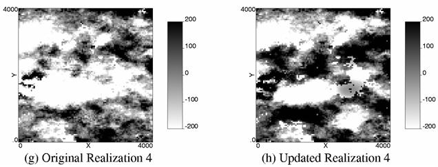
72 Figure 4.23: Permeability difference between true and the conditional realizations. 6

73 Figure 4.24: Histograms of permeability difference between true and the conditional realizations. 61

74 4.4 Sensitivity Study The sensitivity study here focuses on the effects of type of perturbation propagation, perturbation locations and range Effect of Propagation Type The sensitivity study on the effect of propagation type on mismatch was conducted with realization #2. The perturbation locations were selected at 16 locations shown in Figure Figure 4.25: Perturbation locations and well locations. Spherical type and Gaussian type of propagation were selected with the range of 5 meters. Two iterations were selected with the perturbation locations F and H. The results are shown in Figure The mismatch of the updated model with Gaussian types of perturbation propagation reaches lower levels, which means that the Gaussian type of propagation is better in this case. 62

75 1 Mismatch Ratio against Base Case(%) Gaussian type propagation Spherical type propagation Iteration Figure 4.26: Mismatch change for different propagation types Effect of Perturbation Locations A sensitivity study on effect of the order of perturbation locations was conducted with realization #2, range of 5m and the propagation of Gaussian type. The perturbation locations were selected at 16 locations shown in Figure Two different ways were used in the application: one is to perturb the locations near wells at first, and the other is to perturb the locations far away from the wells at first. Seven perturbation locations far away from the wells and nine locations near the wells were selected for both of the two ways. The rule of selecting the perturbation locations near the wells is to select the location nearest to the well with the highest mismatch so that some locations were selected twice while some other locations were not selected. The rule of selecting the perturbation locations far away from wells is to select the location from the south to the north and from the east to west. Figure 4.27 shows the mismatch change for the different orders of selected perturbation locations. Figure 4.27(a) corresponds to the case that the perturbations far from well locations were selected at first; Figure 4.27(b) corresponds to the case that the perturbations near well locations were selected at first. The mismatch results in Figure 4.27(b) are better because of the lower levels of pressure mismatch and rate mismatch as well as global mismatch. 63

76 12 Mismatch Ratio against Base Case(%) Pressure mismatch Rate mismatch Global mismatch Iteration (a) Perturbations far from well locations at first (from the first to the last iteration: J, K,L,M,N,O,P,H,F,D,E,G,F,D,H,I) Mismatch Ratio against Base Case(%) Pressure mismatch Rate mismatch Global mismatch Iteration (b) Perturbations near well locations at first (from the first to the last iteration: H,F,D,E,G,I,H,F,D,J,K,L,M,N,O,P) Figure 4.27: Mismatch versus iteration in the application with different orders of the selected perturbation locations. 64

77 4.4.3 Effect of the Range of Perturbation Propagation A sensitivity study on effect of the range of perturbation propagation was conducted with realization #2, first selection of the locations near wells and the propagation of Gaussian type for perturbation. The perturbation locations were selected at 16 locations shown in Figure 4.27(b). Figure 4.28 shows the mismatch change for the different ranges of propagation. Figure 4.28(a) corresponds to the case that the range of 4m; Figure 4.28(b) corresponds to the case that the range of 5m, which is half the well spacing in the rows from the south to the north. The results show that half the well spacing is a better option for the range of perturbation propagation Pressure mismatch Pressure mismatch Mismatch Ratio against Base Case(%) Rate mismatch Global mismatch Mismatch Ratio against Base Case(%) Rate mismatch Global mismatch Iteration (a) Range of 4m Iteration (b) Range of 5m Figure 4.28: Mismatch versus iteration for different ranges of perturbation propagation Effect of Porosity Model A sensitivity study on effect of the porosity model was conducted with the conditional realization #1, selection of the locations near wells at first and the propagation of Gaussian type. In the methodology, there are two flow simulations at each iteration. One perturbation location is selected to perturb the permeability, then the first flow simulation runs with the perturbed permeability and porosity from the previous iteration. Then, the sensitivities with respect to the permeability change were calculated, which are used to get the optimal changes to update the permeability. After that, the porosity model is 65

78 obtained by two different ways: (1) keeping the same model as the previous iteration, and (2) doing co-simulation with the updated permeability. The second flow simulation runs with the updated porosity and the updated permeability to check the well/reservoir behaviours. Three cases were studied here. Firstly, the permeability realization #1 was updated by the methodology when the true porosity was used with the range of perturbation propagation of 5m. The perturbation locations are the perturbation locations for Figure 4.27(b) plus four locations successively selected near the well with the highest mismatch. The mismatch results are shown in Figure 4.29(a). This is Case 1. Secondly, the permeability realization #1 was updated by the methodology with co-simulated porosity and the same other settings as Case 1. The mismatch results are shown in Figure 4.29(b). This is Case 2. Finally, increasing the number of perturbation locations and enlarging the range of propagate perturbations may reduce the mismatch levels, the permeability conditional realization #1 was updated by the methodology with co-simulated porosity, perturbation locations shown in Figure 4.15 plus one location near the well with the highest mismatch after nineteen iterations, and anisotropy ranges of 5m in the Y direction and 8m in the X direction. The mismatch results are shown in Figure 4.29(c). This is Case 3. The comparison of the three cases is shown in Table 4.6. Table 4.6: Comparison of the three cases. Case Porosity Perturbation Locations Range Original Mismatch Updated Mismatch X Y Pressure Rate Pressure Rate 1 True Figure Co-simulated Figure Co-simulated Figure From Figure 4.29 and Table 4.6, it can be seen that the porosity model has a large effect on mismatch change with iteration and the cases with co-simulated porosity reached a higher mismatch levels than with true porosity. This is expected. Co-simulated porosity is reasonable in practice. The case with the anisotropy ranges got a lower mismatch level for the updated realizations. 66

79 Mismatch Ratio against Base Case(%) Pressure mismatch Rate mismatch Global mismatch Iteration (a) Case 1 12 Mismatch Ratio against Base Case(%) Pressure mismatch Rate mismatch Global mismatch Iteration (b) Case 2 Mismatch Ratio against Base Case(%) Pressure mismatch Rate mismatch Global mismatch Iteration (c) Case 3 Figure 4.29: Mismatch change with iterations for the three different cases. 67

80 4.5 Comparison of Linear Approximation and Flow Simulation Results The linearized formulas of reservoir behaviors (pressure and flow rate) with the property change used for optimization in the methodology, Equations 3.24 to 3.29, are based on the linear assumption of their relationship. The calculated results from the linearized formulas vs. the simulation results at the two iterations in one application to the original permeability realization #1, iteration 5 and iteration 12, are shown in Figures 4.3 and Only the graphs with visible difference between the linear approximation and the simulation results are shown. Figures 4.3 and 4.31 show that the reservoir behaviors obtained by means of the linear approximation and flow simulation are very close in the view of the mismatch calculation, which means that using the linear approximation of reservoir behavior in the optimization of the proposed methodology is suitable WOPR for Pro5 (m 3 /d) 2 1 History Original model Updated model Results from linear formula WOPR for Pro5 (m 3 /d) 2 1 History Original model Updated model Results from linear formula Time (days) Time (days) (a) Well Pro5, Iteration 5 (b) Well Pro5, Iteration WOPR for Pro6 (m 3 /d) History Original model Updated model Results from linear formula WOPR for Pro6 (m 3 /d) History Original model Updated model Results from linear formula Time (days) Time (days) (c) Well Pro6, Iteration 5 (d) Well Pro6, Iteration 12 Figure 4.3: Comparison of the well production rates from linear approximation and simulation results for the updated model. 68

81 WBHP for Pro5 (bar) History Original model Updated model Results from linear formula Time (days) (a) Pro5, Iteration 5 4 WBHP for Pro6 (bar) History Original model Updated model Results from linear formula Time (days) (b) Pro6, Iteration 12 Figure 4.31: Comparison of the well bottom hole pressure from linear approximation and simulation results for the updated model. 69

82 Chapter 5 Application to a North Sea Reservoir This chapter presents the application of the methodology proposed in Chapter 3 to a North Sea reservoir with realistically complex geologic structure and production history. The details of the field are not fully disclosed because they are not necessary; the main point of the chapter is to demonstrate the practical applicability of the methodology. The proposed methodology improves the global mismatch of the reservoir. The fractional flow rate was matched better than pressure. The proposed method can post-process multiple realizations to similar low levels of mismatch. The well settings have a large affect on the calculated pressure values. The use of multiple perturbation locations at each iteration and the choice of suitable multipliers of pore volume and permeability make the methodology more efficient but does not significantly change the final results. Section 5.1 provides the basic information and parameter settings. Section 5.2 gives the results of the application and a sensitivity study on some implementation aspects. 5.1 Basic Information and Parameter Settings There are 9 active wells in the reservoir, where 3 wells were converted into injectors, two wells were shut-in and there are four new wells. ECLIPSE was used for simulation. There are 235,8 grid blocks in the property models. The liquid production rate and water injection rate were input parameters in flow simulation. The well bottom hole pressure and the quarterly averaged oil production rate were the parameters to match. The permeability models were updated. The porosity model was fixed. Two base realizations with different means were considered (Model A and Model B). The horizontal permeability values in the X and Y directions were set to be the same. The 7

83 horizontal permeability in the X direction is highly correlated to the permeability in the Z direction with a correlation coefficient of.91. Therefore, one factor was used to perturb all three permeability models. Flow simulation needs schedule file to set well bore conditions and production rate scheme. Two well schedule files with different well production index settings were considered (Schedule A and Schedule B unrelated to Model A/B). Since there are only 9 active wells in the reservoir, only one perturbation location per iteration was selected. The general principle is to select the perturbation location at a location with high mismatch. The weights for pressure and fractional flow rate were set the same: w p = w q =1. The weight (for mismatch) at each well was obtained from the ratio of the total working time (production and injection) of the well over the sum of the working time of all wells. The historical oil production rates were equally weighted. The weights for well bottom hole pressure were set to the ratio of effective time of each observed datum against the total effective time of all data at that well. The effective time of the first datum or last data was set as two times of the period from the time measuring the data to the middle between time for measuring this datum and the adjacent datum. The total effective time of all data was the sum of the effective time of each datum. The effective time of other datum was defined by the period from the middle of times for measuring this datum and the previous datum to the middle between times for measuring this datum and the next datum. The reservoir is water-wet, stratified and the simulation is liquid rate controlled; therefore, in general, an increase in permeability around a producer tends to increase the water production rate and decrease the oil production rate at the well after water breakthrough. This was used to select the perturbations and to accelerate convergence. 5.2 Results of the Application and Sensitivity Studies The change of the global mismatch of reservoir with iterations and change of mismatch at each well with iterations are presented. The effects of the base model and schedule file, well production index, multipliers of pore volume and permeability, perturbation numbers and locations at each iteration, perturbation propagation variogram and range as well as sensitivity coefficient change with iteration and variogram are studied. 71

84 5.2.1 Change of Global Mismatch of Reservoir with Iterations The methodology was used to update Model A with Schedule A. One perturbation location was selected at each iteration, as shown in Figure 5.1. Figure 5.1: Perturbation locations in the application of the methodology to Model A with Schedule A. The perturbations were propagated to the entire grid system with a spherical type of variogram and a range of 4 grid blocks for iterations 1 to 5 and 3 grid blocks (about half the average well spacing) for iterations 6 to 8. The global mismatch values are shown in Figure 5.2. The global mismatch decreases with iterations. The pressure and rate mismatch for the initial model are 1658 bar 2 and 138 (m 3 /d) 2. After the eighth iteration, the mismatch in oil production rates for the updated model decreased by 8% from the initial model, the mismatch in pressure decreased by 8%. The global mismatch decreased by 44%. 72

85 Mismatch Ratio: Updated Model/Base Model (%) Pressure mismatch Rate mismatch Global mismatch Iteration Figure 5.2: Mismatch change with iterations for Model A with Schedule A. This methodology was applied to Model B with Schedule B. The perturbation locations are shown in Figure 5.3. The results of mismatch change with iterations are shown in Figure 5.4. The pressure and rate mismatch for the initial model are 2592 bar 2 and 193 (m 3 /d) 2. After the 1 th iteration, the mismatch in the fractional flow rate decreased by 8%. The pressure mismatch decreased by 16%. The global mismatch decreases by 48%. Figure 5.3: Perturbation locations in application of the methodology to Model B with Schedule B. 73

86 Mismatch Ratio: Updated Model/Base Model (%) Pressure mismatch Rate mismatch Global mismatch Iteration Figure 5.4: Mismatch change with iterations for the updated Model B with Schedule B. The proposed methodology can reduce pressure and rate mismatch. In the application, rate mismatch for the updated reservoir models is improved much more than pressure mismatch. The comparison of pressure and rate mismatch in real units between the initial and updated models is shown in Table 5.1. The mismatch levels in pressure and rate for the updated models are very close although mismatch levels are different for initial models. Table 5.1: Comparison of initial model and updated models in real units. Mismatch Pressure Rate Model Model A with Schedule A Initial Updated Model B with Schedule A Initial Updated Model A with Schedule B Initial Updated Model B with Schedule B Initial Updated

87 5.2.2 Change of Mismatch at Each Well with Iterations It is difficult to improve the mismatch at all wells and all times at every iteration. This can be seen by comparing the mismatch at each well, as shown in Table 5.2. Some changes at the perturbation locations may make some wells match better but make others match worse. This is because the water injection rate is fixed in the ECLIPSE model so that increasing permeability around a producer tends to increase the water rate at the well but decrease water rate at adjacent wells that are connected to the same injector. Table 5.2: Pressure and rate mismatch at each well for base Model A with Schedule A. Item Iteration Well 1 Well 2 Well 3 Well 4 Well 5 Well 6 Well 7 Well 8 Well Pressure Mismatch Rate Mismatch Global Mismatch better worse better better worse better better worse worse better better worse better better better better better better better better worse better fixed better fixed better worse It can be seen from Table 5.2 that the mismatch in oil production rate at all wells for the updated model after the eighth iteration is smaller than the base model except Well 3. The match in pressure for the updated model at wells 2, 5, 8 and 9 are worse than the base model. The global mismatch at Wells 3 and 9 for the updated model are worse than those for the base model. The perturbation locations were not set near Wells 2 and 3 so 75

88 that the changes of production behaviors of the wells are small no matter how the property at the perturbation location changes. Well 5 is a new producer with a short working time. The curves of pressure and oil production rates at the four wells are shown in Figure 5.5. The mismatch in oil production rates and pressure at Well 1 are improved and can be seen from the figures. Well 4 is a new producer and the mismatch in oil production rates and pressure at the well are improved but hard to see the improvement of pressure mismatch from the figure. Well 6 is an old producer and the mismatch in oil production rate at the well is improved but the pressure observations are too few so that the improvement of the pressure mismatch can not been seen. Well 9 got an almost perfect match in oil production rate but a worse match in pressure between observed data and simulation results. Wells 8 and 9 were producers at the beginning of the development and are injectors now. The well production indices and skin factors have a large effect on the well bottom-hole pressure. Wells 8 and 9 experienced stimulation work but their well production indexes were set as constant in Schedule file A; updating those values would improve the match (see Section 5.2.4) Effect of Base Model and Schedule File The methodology was applied to two sets of property models and schedule files. The results in Figure 5.6 show that the proposed methodology can be used to build property models corresponding to a similar global mismatch from the different initial realizations with the same schedule files. The global mismatch with different schedule files converge to different mismatch levels. Setting appropriate well conditions is important. The final images in the area with the wells are consistent between multiple updated realizations, as shown in Figure Effect of Well Production Index on Pressure Mismatch The well production index (WPI) is a parameter that has a large effect on simulated well performance. Considering that well production index at Well 9 may be changed around time of 61 and the historical pressure is higher than the simulation results of the updated model after that time, the changing of well production index at Well 9 from 3. to 2.5 in the Schedule A improved the mismatch in pressure at the well, see Figure 5.8. The well production index has little effect on mismatch in oil production rates. 76

89 3 4 WOPR for Well History Base model A Updated model A WBHP for Well History Base model A Updated model A Time Time (a) WOPR, Well 1 (b) WBHP, Well WOPR for Well History Base model A Updated model A WBHP for Well History Base model A Updated model A Time Time (c) WOPR, Well 4 (d) WBHP, Well WOPR for Well History Base model A Updated model A WBHP for Well History Base model A Updated mode Al Time Time (e) WOPR, Well 6 (f) WBHP, Well WOPR for Well History Base model A Updated model A WBHP for Well History Base model A Updated model A Time Time (g) WOPR, Well 9 (h) WBHP, Well 9 Figure 5.5: The curves of oil production rates and well bottom-hole pressure at the four wells for the Original Model A and Updated Model A with Schedule A. 77

90 1 Global Mismatch/Mismatch of Base Model B with Schedule B (%) Model A, Schedule B Model A, Schedule A Model B, Schedule B Model B, Schedule A Iteration Figure 5.6: Global mismatch of the updated models started from the different combinations of property models and schedule files. (a) Model A (b) Model B (c) Updated Model A (d) Updated Model B Figure 5.7: Maps of permeability in the X direction in the top layer for the two base models and their updated models. 78