A Crash Course on Kalman Filtering

Transcription

1 A Crash Course on Kalman Filtering Dan Simon Cleveland State University Fall / 64

2 Outline Linear Systems Probability State Means and Covariances Least Squares Estimation The Kalman Filter Unknown Input Estimation The Extended Kalman Filter 2 / 64

3 Linear Systems KVL: u = v c + L di L /dt KCL: i c + i r1 = i r2 + i L i c = C dv c /dt i r1 = v c /R i r2 = (u v c )/R = dv c /dt = 2v c /RC + i L /C + u/rc Define x T = [ ] v c i [ L ] [ ] 2/RC 1/C 1/RC ẋ = x + u = Ax + Bu 1/L 0 1/L What is the output? Suppose y = v r2 = L di L /dt = [ 1 0 ] x + u = Cx + Du 3 / 64

4 Linear Systems Let R = C = L = 1 and u(t) = step function. How can we simulate the system in Matlab? Control System Toolbox Simulink m-file 4 / 64

5 Linear Systems: Continuous-Time Simulation Control System Toolbox: R = 1; L = 1; C = 1; A = [-2/R/C, 1/C ; -1/L, 0]; B = [1/R/C ; 1/L]; C = [-1, 0]; D = 1; sys = ss(a, B, C, D); step(sys) Simulink: LinearRLC1Model.slx m-file: LinearRLC1.m What time step should we use? 5 / 64

6 Linear Systems: Discretization Continuous time: ẋ = Ax + Bu, y = Cx + Du Discrete time: x k+1 = Fx + Gu, y = Cx + Du F = exp(a t) G = (F I )A 1 B where t is the integration step size; I is the identity matrix 6 / 64

7 Linear Systems: Discrete-Time Simulation Control System Toolbox: dt = 0.1; F = expm(a*dt); G = (F - eye(2)) / A * B; sysdiscrete = ss(f, G, C, D, dt); step(sysdiscrete) Simulink: LinearRLC1DiscreteModel.slx m-file: LinearRLC1Discrete.m 7 / 64

8 Outline Linear Systems Probability State Means and Covariances Least Squares Estimation The Kalman Filter Unknown Input Estimation The Extended Kalman Filter 8 / 64

9 Cumulative Distribution Function X = random variable CDF: F X (x) = P(X x) F X (x) [0, 1] F X ( ) = 0 F X ( ) = 1 F X (a) F X (b) if a b P(a < X b) = F X (b) F X (a) 9 / 64

10 Probability Density Function PDF: f X (x) = df X (x) dx F X (x) = f X (x) 0 f X (x) dx = 1 P(a < x b) = Expected value: E[g(X )] = x b a f X (z) dz f X (x) dx g(x)f X (x) dx E(X ) = x = µ x = mean E [ (X x) 2] = σx 2 = variance σ x = standard deviation 10 / 64

11 Probability Random numbers in Matlab: rand and randn Random number seed How can we create a random vector with given covariance R? Probability Density Functions Uniform Distribution Gaussian, or Normal, Distribution 11 / 64

12 Multiple Random Variables Independence: CDF: F XY (x, y) = P(X x, Y y) PDF: f XY (x, y) = 2 F XY (x, y) x y P(X x, Y y) = P(X x)p(y y) for all x, y Covariance: C XY = E[(X X )(Y Ȳ ] = E(XY ) X Ȳ Correlation: R XY = E(XY ) 12 / 64

13 Random Vectors X = [ X 1 X 2 ] CDF: F X (x) = P(X 1 x 1, X 2 x 2 ) pdf: f X (x) = 2 F X (x) x 1 x 2 Autocorrelation: R X = E[XX T ] > 0 Autocovariance: C X = E[(X X )(X X ) T ] > 0 Gaussian RV: PDF(x) = [ ] 1 1 (2π) n/2 exp C X 1/2 2 (x x)t C 1 X (x x) If Y = AX + b, then Y N(A x + b, AC X A T ) 13 / 64

14 Stochastic Processes A stochastic process X (t) is an RV that varies with time If X (t 1 ) and X (t 2 ) are independent t 1 t 2 then X (t) is white Otherwise, X (t) is colored Examples: The high temperature on a given day The closing price of the stock market Measurement noise in a voltmeter The amount of sleep you get each night 14 / 64

15 Outline Linear Systems Probability State Means and Covariances Least Squares Estimation The Kalman Filter Unknown Input Estimation The Extended Kalman Filter 15 / 64

16 State Means and Covariances x k = F k 1 x k 1 + G k 1 u k 1 + w k 1 w k (0, Q k ) x k = E(x k ) = F k 1 x k 1 + G k 1 u k 1 (x k x k )( ) T = (F k 1 x k 1 + G k 1 u k 1 + w k 1 x k )( ) T = [F k 1 (x k 1 x k 1 ) + w k 1 ][ ] T = F k 1 (x k 1 x k 1 )(x k 1 x k 1 ) T F T k 1 + w k 1 w T k 1 + F k 1(x k 1 x k 1 )w T k 1 + w k 1 (x k 1 x k 1 ) T Fk 1 T P k = E [(x ] k x k )( ) T = F k 1 P k 1 F T k 1 + Q k 1 This is the discrete-time Lyapunov Equation, or Stein Equation 16 / 64

17 Outline Linear Systems Probability State Means and Covariances Least Squares Estimation The Kalman Filter Unknown Input Estimation The Extended Kalman Filter 17 / 64

18 Least Squares Estimation Suppose x is a constant vector Vector measurement at time k: y k = H k x + v k, v k (0, R k ) Estimate: ˆx k = ˆx k 1 + K k (y k H k ˆx k 1 ) This is a recursive estimator re cur sive: adjective, meaning recursive Our goal: Find the best estimator gain K k 18 / 64

19 Least Squares Estimation What is the mean of the estimation error? E(ɛ x,k ) = E(x ˆx k ) = E[x ˆx k 1 K k (y k H k ˆx k 1 )] = E[ɛ x,k 1 K k (H k x + v k H k ˆx k 1 )] = E[ɛ x,k 1 K k H k (x ˆx k 1 ) K k v k ] = (I K k H k )E(ɛ x,k 1 ) K k E(v k ) E(ɛ x,k ) = 0 if E(v k ) = 0 and E(ɛ x,k 1 ) = 0, regardless of K k Unbiased estimator 19 / 64

20 Least Squares Estimation Objective function: J k = E[(x 1 ˆx 1 ) 2 ] + + E[(x n ˆx n ) 2 ] = E ( ɛ 2 x1,k + + ) ɛ2 xn,k ( ) = E ɛ T x,k ɛ x,k ] = E [Tr(ɛ x,k ɛ T x,k ) = Tr P k 20 / 64

21 Least Squares Estimation P k = E(ɛ x,k ɛ T x,k ) = E {[(I } K k H k )ɛ x,k 1 K k v k ][ ] T = (I K k H k )E(ɛ x,k 1 ɛ T x,k 1 )(I K kh k ) T K k E(v k ɛ T x,k 1 )(I K kh k ) T (I K k H k )E(ɛ x,k 1 vk T )K k T + K k E(v k vk T )K k T = (I K k H k )P k 1 (I K k H k ) T + K k R k Kk T 21 / 64

22 Least Squares Estimation Recall that Tr(ABAT ) A = 2AB if B is symmetric J k K k = 2(I K k H k )P k 1 ( Hk T ) + 2K kr k = 0 K k R k = (I K k H k )P k 1 H T k K k (R k + H k P k 1 Hk T ) = P k 1Hk T K k = P k 1 Hk T (H kp k 1 Hk T + R k) 1 22 / 64

23 Recursive least squares estimation of a constant 1 Initialization: ˆx 0 = E(x), P 0 = E[(x ˆx 0 )(x ˆx 0 ) T ] If no knowledge about x is available before measurements are taken, then P 0 = I. If perfect knowledge about x is available before measurements are taken, then P 0 = 0. 2 For k = 1, 2,, perform the following. 1 Obtain measurement y k : y k = H k x + v k where v k (0, R k ) and E(v i v k ) = R k δ k i (white noise) 2 Measurement update of estimate: K k = P k 1 H T k (H k P k 1 H T k + R k ) 1 ˆx k = ˆx k 1 + K k (y k H k ˆx k 1 ) P k = (I K k H k )P k 1 (I K k H k ) T + K k R k K T k 23 / 64

24 Alternate Estimator Equations K k = P k 1 H T k (H kp k 1 H T k + R k) 1 = P k H T k R 1 k P k = (I K k H k )P k 1 (I K k H k ) T + K k R k Kk T = (P 1 H k) 1 Example: RLS.m k 1 + HT k R 1 k = (I K k H k )P k 1 (Valid only for optimal K k ) 24 / 64

25 Outline Linear Systems Probability State Means and Covariances Least Squares Estimation The Kalman Filter Unknown Input Estimation The Extended Kalman Filter 25 / 64

26 The Kalman filter x k = F k 1 x k 1 + G k 1 u k 1 + w k 1 y k = H k x k + v k w k (0, Q k ) v k (0, R k ) E[w k wj T ] = Q k δ k j E[v k vj T ] = R k δ k j E[v k wj T ] = 0 ˆx + k = E[x k y 1, y 2,, y k ] = a posteriori estimate P + k = E[(x k ˆx + k )(x k ˆx + k )T ] ˆx k = E[x k y 1, y 2,, y k 1 ] = a priori estimate P k = E[(x k ˆx k )(x k ˆx k )T ] ˆx k k+n = E[x k y 1, y 2,, y k,, y k+n ] = smoothed estimate ˆx k k M = E[x k y 1, y 2,, y k M ] = predicted estimate 26 / 64

27 Time Update Equations Initialization: ˆx 0 + = E(x 0 ) ˆx 1 = F 0ˆx G 0u 0 P1 = F 0 P 0 + F 0 T + Q 0 Generalize: ˆx k = F k 1ˆx + k 1 + G k 1u k 1 P k = F k 1 P + k 1 F k 1 T + Q k 1 These are the Kalman filter time update equations 27 / 64

28 Measurement Update Equations Recall the RLS estimate of a constant x: K k = P k 1 H T k (H kp k 1 H T k + R k) 1 ˆx k = ˆx k 1 + K k (y k H k ˆx k 1 ) P k = (I K k H k )P k 1 (I K k H k ) T + K k R k K T k ˆx k 1, P k 1 = estimate and covariance before measurement y k ˆx k, P k = estimate and covariance after measurement y k Least squares estimator Kalman filter ˆx k 1 = estimate before y k = ˆx k = a priori estimate P k 1 = covariance before y k = P k = a priori covariance ˆx k = estimate after y k = ˆx + k = a posteriori estimate P k = covariance after y k = P + k = a posteriori covariance 28 / 64

29 Measurement Update Equations Recursive Least Squares: K k = P k 1 Hk T (H kp k 1 Hk T + R k) 1 ˆx k = ˆx k 1 + K k (y k H k ˆx k 1 ) P k = (I K k H k )P k 1 (I K k H k ) T + K k R k Kk T Kalman Filter: K k = P k HT k (H kp k HT k + R k) 1 ˆx + k = ˆx k + K k(y k H k ˆx k ) P + k = (I K k H k )P k (I K kh k ) T + K k R k Kk T These are the Kalman filter measurement update equations 29 / 64

30 Kalman Filter Equations 1 State equations: x k = F k 1 x k 1 + G k 1 u k 1 + w k 1 y k = H k x k + v k E(w k wj T ) = Q k δ k j, E(v k vj T ) = R k δ k j, E(w k vj T ) = 0 2 Initialization: ˆx + 0 = E(x 0), P + 0 = E[(x 0 ˆx + 0 )(x 0 ˆx + 0 )T ] 3 For each time step k = 1, 2, P k = F k 1 P + k 1 F T k 1 + Q k 1 K k = P k HT k (H kp k HT k + R k) 1 = P + k HT k R 1 k ˆx k = F k 1ˆx + k 1 + G k 1u k 1 = a priori state estimate ˆx + k = ˆx k + K k(y k H k ˆx k ) = a posteriori state estimate P + k = (I K k H k )P k (I K kh k ) T + K k R k Kk T [ ] 1 = (P k ) 1 + Hk T R 1 k H k = (I K k H k )P k 30 / 64

31 Kalman Filter Properties Define estimation error x k = x k ˆx k Problem: min E [ x T k S k x k ], where Sk > 0 If {w k } and {v k } are Gaussian, zero-mean, uncorrelated, and white, then the Kalman filter solves the problem. If {w k } and {v k } are zero-mean, uncorrelated, and white, then the Kalman filter is the best linear solution to the problem. If {w k } and {v k } are correlated or colored, then the Kalman filter can be easily modified to solve the problem. For nonlinear systems, the Kalman filter can be modified to approximate the solution to the problem. 31 / 64

32 Kalman Filter Example: DiscreteKFEx1.m ṙ v ȧ = r v a + w = ẋ = Ax + w x k+1 = Fx k + w k F = exp(at ) = w k (0, Q k ) 1 T T 2 /2 0 1 T ˆx k = F ˆx + k 1 P k = FP + k 1 F T + Q k 1 y k = H k x k + v k = [ ] x k + v k v k (0, R k ), R k = σ 2 32 / 64

33 Kalman Filter Divergence Kalman filter theory is based on several assumptions. How to improve filter performance in the real world: Increase arithmetic precision Square root filtering Use a fading-memory Kalman filter Use fictitious process noise Use a more robust filter (e.g., H-infinity) 33 / 64

34 Modeling Errors True System: x 1,k+1 = x 1,k + x 2,k x 2,k+1 = x 2,k y k = x 1,k + v k v k (0, 1) Incorrect Model: x 1,k+1 = x 1,k y k = x k + v k w k (0, Q), Q = 0 v k (0, 1) 34 / 64

35 Modeling Errors true state estimated state time Figure: Kalman filter divergence due to mismodeling 35 / 64

36 Fictitious Process Noise true state xhat (Q = 1) xhat (Q = 0.1) xhat (Q = 0.01) xhat (Q = 0) time Figure: Kalman filter improvement due to fictitious process noise 36 / 64

37 Fictitious Process Noise Q = 1 Q = 0.1 Q = 0.01 Q = time Figure: Kalman gain for various values of process noise 37 / 64

38 The Continuous-Time Kalman Filter Discretize: ẋ = Ax + Bu + w y = Cx + v w (0, Q c ) v (0, R c ) x k = Fx k 1 + Gu k 1 + w k 1 y k = Hx k + v k F = exp(at ) (I + AT ) for small T G = (exp(at ) I )A 1 B BT for small T H = C w k (0, Q), Q = Q c T v k (0, R), R = R c /T 38 / 64

39 The Continuous-Time Kalman Filter Recall the discrete-time Kalman gain: lim T 0 K k = P k HT (HP k HT + R) 1 K k = P k C T (CP k C T + R c /T ) 1 T = P k C T (CP k C T T + R c ) 1 K k T = P k C T Rc 1 39 / 64

40 The Continuous-Time Kalman Filter Recall the discrete-time estimation error covariance equations: P + k = (I K k H)P k P k+1 = FP + k F T + Q = (I + AT )P + k (I + AT )T + Q c T, for small T = P + k + (AP+ k + P+ k AT + Q c )T + AP + k AT T 2 = (I K k C)P k + AP+ k AT T 2 + [A(I K k C)P k + (I K kc)p k AT + Q c ]T P k+1 P k T = K kcp k + AP + T k AT T + (AP k + AK kcp k + P k AT K k CP k AT + Q c ) Ṗ = P k+1 lim k T 0 T = PC T Rc 1 CP + AP + PA T + Q c 40 / 64

41 The Continuous-Time Kalman Filter Recall the discrete-time state estimate equations: ˆx k = F ˆx + k 1 + Gu k 1 ˆx + k = ˆx k + K k(y k H ˆx k ) = F ˆx + k 1 + Gu k 1 + K k (y k HF ˆx + k 1 HGu k 1) (I + AT )ˆx + k 1 + BTu k 1 + K k (y k C(I + AT )ˆx + k 1 CBTu k 1), for small T = ˆx + k 1 + AT ˆx + k 1 + BTu k 1 + PC T Rc 1 T (y k C ˆx + k 1 CAT ˆx + k 1 CBTu k 1) ˆx ˆx + k = lim T 0 ˆx + k 1 T = Aˆx + Bu + PC T Rc 1 (y C ˆx) ˆx = Aˆx + Bu + K(y C ˆx) K = PC T R 1 c 41 / 64

42 The Continuous-Time Kalman Filter Continuous-time system dynamics and measurement: ẋ = Ax + Bu + w y = Cx + v w (0, Q c ) v (0, R c ) Continuous-time Kalman filter equations: ˆx(0) = E[x(0)] P(0) = E[(x(0) ˆx(0))(x(0) ˆx(0)) T ] K = PC T Rc 1 ˆx = Aˆx + Bu + K(y C ˆx) Ṗ = PC T Rc 1 CP + AP + PA T + Q c What if y includes the input also? That is, y = Cx + Du? 42 / 64

43 Example: Regenerative Knee Prosthesis 43 / 64

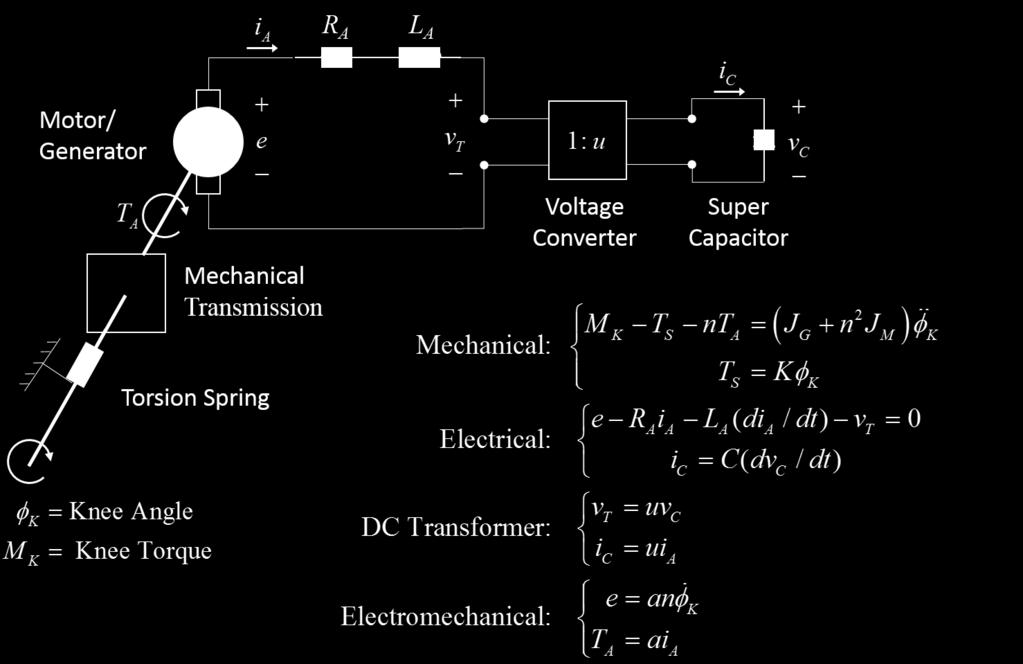
44 System Equations 44 / 64

45 Input Torque M D. Winter, Biomechanics and Motor Control of Human Movement, 4th Edition, Wiley, 2009, Appendix A bcs.wiley.com/he-bcs/books?action=resource&bcsid=5453&itemid= &resourceid= / 64

46 State Equations x 1 = φ k x 2 = φ k x 3 = i A x 4 = v C J T = J G + n 2 J M ẋ = K/J T 0 na/j T 0 0 an/l A R A /L A u/l A 0 0 u/c 0 [ ] y = x + v x + 0 1/J T 0 0 M K + w Matlab program: RegenerationKalman.m 46 / 64

47 Outline Linear Systems Probability State Means and Covariances Least Squares Estimation The Kalman Filter Unknown Input Estimation The Extended Kalman Filter 47 / 64

48 Unknown Input Estimation Continuous-time system dynamics and measurement: Consider f as a state: ẋ = Ax + Bu + f + w y = Cx + v w (0, Q c ), v (0, R c ) z = [ x T f T ] T [ ] [ A I B ż = z y = [ C 0 ] [ v z + 0 ] [ w u + w (0, Q), Q = diag(qc, Q ) v (0, R), R = diag(rc, 0) w is fictitious process noise, and Q is a tuning parameter ] w ] 48 / 64

49 Unknown Input Estimation: Rowing Machine θ = position, ω = velocity, q = capacitor charge k = spring constant, J = inertia, a = motor constant R = resistance, u = power converter ratio, C = capacitance r = radius, φ = friction 49 / 64

50 Unknown Input Estimation: Rowing Machine System model: ] θ = ω ω = k J θ a2 RJ ω + au RCJ q + r φ(θ, ω) F J J q = au R ω u2 RC q, φ(, ) = 0.12sign(ω) State space model, assuming ω > 0: ẋ = k/j a 2 /RJ au/rcj r/j 0 au/r u 2 /RC 0 x [ w (0, Q), Q = diag q 1, q 2, q 3, q 4 y = Cx + v = x + v [ ] v (0, R), R = diag , , (0.01C) 2 + w (q = CV ) 50 / 64

51 Unknown Input Estimation: Rowing Machine Q = diag([0.01 2, , 1 2, 1 2 ]) - not responsive enough 51 / 64

52 Unknown Input Estimation: Rowing Machine Q = diag([0.01 2, , 1 2, ]) - too responsive 52 / 64

53 Unknown Input Estimation: Rowing Machine Q = diag([0.01 2, , 1 2, ]) - just about right 53 / 64

54 Unknown Input Estimation: Rowing Machine How can we improve our results? We have modeled F as a noisy constant: Instead we can model F as a ramp: F = F v + w 1 F v = w 2 F = w This increases the number of states by 1 but gives the Kalman filter more flexibility to estimate a value for F that matches the measurements RMS force estimation error decreases from 0.8 N to 0.4 N 54 / 64

55 Outline Linear Systems Probability State Means and Covariances Least Squares Estimation The Kalman Filter Unknown Input Estimation The Extended Kalman Filter 55 / 64

56 Nonlinear Kalman Filtering Nonlinear system: ẋ = f (x, u, w, t) y = h(x, v, t) w (0, Q) v (0, R) Linearization: ẋ f (x 0, u 0, w 0, t) + f x (x x 0 ) + f 0 u (u u 0 ) + 0 f w (w w 0 ) 0 = f (x 0, u 0, w 0, t) + A x + B u + L w y h(x 0, v 0, t) + h x (x x 0 ) + h 0 v (v v 0 ) 0 = h(x 0, v 0, t) + C x + M v 56 / 64

57 Nonlinear Kalman Filtering ẋ 0 = f (x 0, u 0, w 0, t) y 0 = h(x 0, v 0, t) ẋ = ẋ x 0 y = y y 0 ẋ = A x + Lw = A x + w w (0, Q), Q = LQL T y = C x + Mv = C x + ṽ ṽ (0, R), R = MRM T We have a linear system with state x and measurement y 57 / 64

58 The Linearized Kalman Filter System equations: Nominal trajectory: ẋ = f (x, u, w, t), w (0, Q) y = h(x, v, t), v (0, R) x 0 = f (x 0, u 0, 0, t), y 0 = h(x 0, 0, t) Compute partial derivative matrices: A = f / x 0, L = f / w 0, C = h/ x 0, M = h/ v 0 Compute Q = LQL T, R = MRM T, y = y y 0 Kalman filter equations: ˆx(0) = 0, P(0) = E [( x(0) ] ˆx(0))( x(0) ˆx(0)) T ˆx = A ˆx + K( y C ˆx), K = PC T R 1 Ṗ = AP + PA T + Q PC T R 1 CP ˆx = x 0 + ˆx 58 / 64

59 The Extended Kalman Filter Combine the ẋ 0 and ˆx equations: ẋ 0 + ˆx = f (x 0, u 0, w 0, t) + A ˆx + K[y y 0 C(ˆx x 0 )] Choose x 0 (t) = ˆx(t), so ˆx(t) = 0 and ˆx(t) = 0 Then the nominal measurement becomes y 0 = h(x 0, v 0, t) = h(ˆx, v 0, t) and the first equation above becomes ˆx = f (ˆx, u, w 0, t) + K [y h(ˆx, v 0, t)] 59 / 64

60 The Extended Kalman Filter System equations: ẋ = f (x, u, w, t), w (0, Q) y = h(x, v, t), v (0, R) Compute partial derivative matrices: A = f / x ˆx, L = f / w ˆx, C = h/ x ˆx, M = h/ v ˆx Compute Q = LQL T, R = MRM T Kalman filter equations: ˆx(0) = E[x(0)], P(0) = E [(x(0) ] ˆx(0))(x(0) ˆx(0)) T ˆx = f (ˆx, u, 0, t) + K [y h(ˆx, 0, t)], K = PC T R 1 Ṗ = AP + PA T + Q PC T R 1 CP 60 / 64

61 Robot State Estimation Robot dynamics: u = M q + C q + g + R + F u = control forces/torques, q = joint coordinates M(q) = mass matrix, C(q, q) = Coriolis matrix g(q) = gravity vector, R( q) = friction vector F (q) = external forces/torques State space model: q = M 1 (u C q g R F ) x = [ ] T [ q 1 q 2 q 3 q 1 q 2 q 3 = x T 1 x2 T [ ] x ẋ = 2 M 1 = f (x, u, w, t) (u C q g R F ) y = q 3 = [ ] x + v = h(x, v, t) The detailed model is available at: dynamicsystems.asmedigitalcollection.asme.org/article.aspx?articleid= ] T 61 / 64

62 Robot State Estimation System equations: ẋ = f (x, u, w, t), w (0, Q) y = h(x, v, t), v (0, R) Compute partial derivative matrices: A = f / x ˆx, L = f / w ˆx, C = h/ x ˆx, M = h/ v ˆx Compute Q = LQL T, R = MRM T Kalman filter equations: ˆx(0) = E[x(0)], P(0) = E [(x(0) ] ˆx(0))(x(0) ˆx(0)) T ˆx = f (ˆx, u, 0, t) + K [y h(ˆx, 0, t)], K = PC T R 1 Ṗ = AP + PA T + Q PC T R 1 CP 62 / 64

63 Robot State Estimation: Robot.zip First we write a simulation for the dynamic system model: simgrf.mdl and statederccfforce.m Then we write a controller: PBimpedanceCCFfull.m Then we calculate the A matrix: CalcFMatrix.m and EvaluateFMatrix.m Then we write a Kalman filter: zhatdot.m Run the program: Run setup.m Run simgrf.mdl Look at the output plots: Run plotter.m to see control performance Open Plotting - 1 meas block to see estimator performance Open the q1, q1hat scope to see hip position Open the q2, q2hat scope to see thigh angle Open the q3meas, q3, q3hat scope to see knee angle 63 / 64

64 Additional Estimation Topics Nonlinear estimation Iterated EKF Second-order EKF Unscented Kalman filter Particle filter Many others... Parameter estimation Smoothing Adaptive filtering Robust filtering (H filtering) Constrained filtering 64 / 64