A SARIMAX coupled modelling applied to individual load curves intraday forecasting

Transcription

1 A SARIMAX coupled modelling applied to individual load curves intraday forecasting Frédéric Proïa Workshop EDF Institut Henri Poincaré - Paris 05 avril 2012 INRIA Bordeaux Sud-Ouest Institut de Mathématiques de Bordeaux 1 / 40

2 Plan 1 Introduction 2 On a SARIMAX coupled modelling Stationary ARMA processes Identification for stationary AR(p) and MA(q) processes Linear relationship between consumption and temperature The SARIMAX modelling Application to forecasting 3 Application to forecasting on a load curve Procedure Seasonality and stationarity ACF and PACF Selection criteria Selection on bayesian criteria Selection on bayesian criteria 4 Application on a huge dataset Technical issues Procedure Modelling Forecasting 5 Conclusion 2 / 40

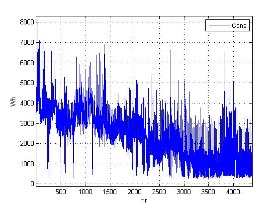
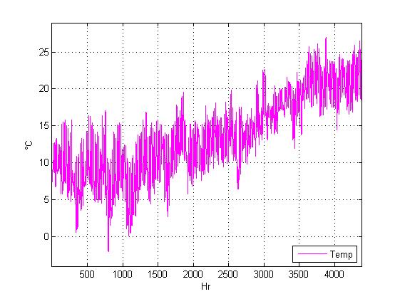
3 Introduction Motivations. New energy meters to gather individual consumption with high frequencie. Economic issue for EDF : anticipate to optimize. Objectives. Distinguish nonthermosensitive from thermosensitive customers. Intraday daily forecasting. Introduce temperature as an exogenous contribution. 3 / 40

4 Introduction Detecting thermosensitivity. Deterministic criterion. Thermosensitivity if max Mt min t N t N Mt > δ where M t is the empirical median of ( C t... ) C t +1. = 1440 et δ = More pertinent than SR/DR. 70% of nonthermosensitive customers, only including 75% of SR. 4 / 40

5 Plan 1 Introduction 2 On a SARIMAX coupled modelling Stationary ARMA processes Identification for stationary AR(p) and MA(q) processes Linear relationship between consumption and temperature The SARIMAX modelling Application to forecasting 3 Application to forecasting on a load curve Procedure Seasonality and stationarity ACF and PACF Selection criteria Selection on bayesian criteria Selection on bayesian criteria 4 Application on a huge dataset Technical issues Procedure Modelling Forecasting 5 Conclusion 5 / 40

6 On a SARIMAX coupled modelling Stationary ARMA processes Stationary ARMA processes. Definition (Stationarity) A time series (Y t ) is said to be weakly stationary if, for all t Z, E[Y 2 t ] <, E[Y t ] = m and, for all s, t Z, Cov(Y t, Y s) = Cov(Y t s, Y 0 ). Definition (ARMA) Let (Y t ) be a stationary time series with zero mean. It is said to be an ARMA(p, q) process if, for every t Z, p q Y t a k Y t k = ε t + b k ε t k k=1 k=1 where (ε t ) is a white noise of variance σ 2 > 0, a R p and b R q. 6 / 40

7 On a SARIMAX coupled modelling Stationary ARMA processes Causality of ARMA processes. Compact expression, for all 1 t T, where the polynomials A(B)Y t = B(B)ε t A(z) = 1 a 1 z... a pz p and B(z) = 1 + b 1 z b qz q. Definition (Causality) Let (Y t ) be an ARMA(p, q) process for which the polynomials A and B have no common zeroes. Then, (Y t ) is causal if and only if A(z) 0 for all z C such that z 1. Implications. Causality implies the existence of a MA( ) structure for (Y t ). Causality implies stationarity of the process. On N, causality often coincides with stationarity. 7 / 40

8 On a SARIMAX coupled modelling Stationary ARMA processes Existence and unicity of a stationary solution. Proposition If A(z) 0 for all z C such that z 1, then the ARMA equation A(B)Y t = B(B)ε t have the unique stationary solution Y t = ψ k ε t k, k=0 and the coefficients (ψ k ) k N are determined by the relation A 1 (z)b(z) = ψ k z k k=0 with ψk 2 <. k=0 Explosive cases. On Z, no zeroes on the unit circle is a sufficient condition. Irrelevant for practical purposes. 8 / 40

9 On a SARIMAX coupled modelling Identification for stationary AR(p) and MA(q) processes Autocorrelation function. To identify q. Definition (ACF) Let (Y t ) be a stationary time series. The autocorrelation function ρ associated with (Y t ) is defined, for all t Z, as ρ(t) = γ(t) γ(0) where the autocovariance function γ(t) = Cov(Y t, Y 0 ). Proposition The stationary time series (Y t ) with zero mean is a MA(q) process such that b q 0 if and only if ρ(q) 0 and ρ(t) = 0 for all t > q. 9 / 40

10 On a SARIMAX coupled modelling Identification for stationary AR(p) and MA(q) processes Examples. MA(1) : only ρ(1) nonzero, exponential decay of α(t). MA(2) : only ρ(1) and ρ(2) nonzero, damped exponential and sine wave for α(t). 10 / 40

11 On a SARIMAX coupled modelling Identification for stationary AR(p) and MA(q) processes Partial autocorrelation function. To identify p. Definition (PACF) Let (Y t ) be a stationary time series with zero mean. The partial autocorrelation function α is defined as α(0) = 1, and, for all t N, as α(t) = φ t, t where (φ t, t ) t N are computed via the Durbin-Levinson recursion. Proposition If there exists a square-integrable sequence (ψ k ) k N such that (Y t ) has a MA( ) expression with ψ 0 = 1, then the stationary time series (Y t ) with zero mean is an AR(p) process such that a p 0 if and only if α(p) 0 and α(t) = 0 for all t > p. 11 / 40

12 On a SARIMAX coupled modelling Identification for stationary AR(p) and MA(q) processes Examples. AR(1) : only α(1) nonzero, exponential decay of ρ(t). AR(2) : only α(1) and α(2) nonzero, damped exponential and sine wave for ρ(t). 12 / 40

13 On a SARIMAX coupled modelling Identification for stationary AR(p) and MA(q) processes Examples. ARMA(1,1) : exponential decay of ρ(t) and α(t) from first lag. ARMA(2,2) : exponential decay of ρ(t) and α(t) from second lag. 13 / 40

14 On a SARIMAX coupled modelling Linear relationship between consumption and temperature Variance-stabilizing Box-Cox transformation. Logarithmic transform given, for all 1 t T, by Y t = log ( C t + e m) where m ensures that Y t = m when C t = / 40

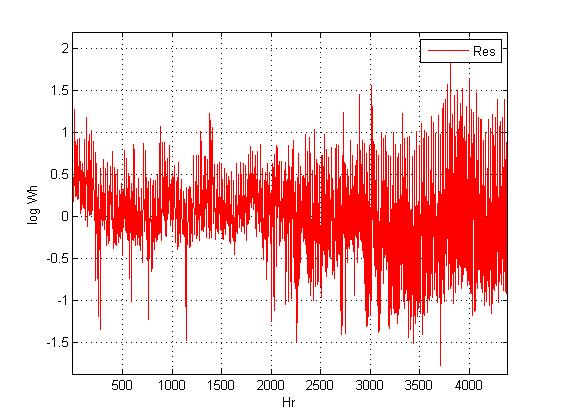
15 On a SARIMAX coupled modelling Linear relationship between consumption and temperature Linear relationship between consumption and temperature. On a thermosensitive load curve, for all 1 t T, For all z C, Y t = c 0 + C(B)U t + ε t. r 1 C(z) = c k+1 z k. k=0 Unknown vector c R r+1 estimated by OLS. Seasonal residuals. Residuals (ε t ) regarded as a seasonal time series. 15 / 40

16 On a SARIMAX coupled modelling The SARIMAX modelling Residuals (ε t ) as a seasonal time series. SARIMA(p, d, q) (P, D, Q) s modelling, for all 1 t T, (1 B) d (1 B s ) D A(B)A s(b)ε t = B(B)B s(b)v t, where (V t ) is a white noise of variance σ 2 > 0. Polynomials defined, for all z C, as p A(z) = 1 a k z k, k=1 P A s(z) = 1 α k z sk, k=1 B(z) = 1 q b k z k, k=1 B s(z) = 1 Q β k z sk, Parameters a R p, b R q, α R P and β R Q estimated by GLS. A and A s are causal. k=1 16 / 40

17 On a SARIMAX coupled modelling The SARIMAX modelling The dynamic coupled modelling. Definition (SARIMAX) In the particular framework of the study, a random process (Y t ) will be said to follow a SARIMAX(p, d, q, r) (P, D, Q) s coupled modelling if, for all 1 t T, it satisfies { Yt = c 0 + C(B)U t + ε t, (1 B) d (1 B s ) D A(B)A s(b)ε t = B(B)B s(b)v t. As soon as d + D > 0, (1 B) d (1 B s ) D A(B)A s(b) (Y t C(B)U t ) = B(B)B s(b)v t. 17 / 40

18 On a SARIMAX coupled modelling The SARIMAX modelling Existence of a stationary solution. Let I be the identity matrix of order T and 1 U T U T 1... U T r+1 Y 1 1 U T 1 U T 2... U T r Y 2 U =, Y = U 1 U 0... U r+2 Y T Theorem Assume that U U is invertible. Then, the differenced process ( d D s εt ) where εt is given, for all 1 t T, by the vector form ( ε = I U(U U) 1 U ) Y is a stationary solution of the coupled model suitably specified. ADF and KPSS tests : d and D. Box and Jenkins methodology : p, q, r, P, Q, s. 18 / 40

19 On a SARIMAX coupled modelling Application to forecasting Forecasting using time series analysis. Let ε T +1 be the predictor of (ε t ) at stage T + 1. Let ĉ T be the OLS estimate of c. Assume that r has been evaluated. The predictor at horizon 1 is given by Ỹ T +1 = ĉ 0,T + The predictor at horizon H is given by Ỹ T +H = ĉ 0,T + r ĉ k,t U T k+2 + ε T +1. k=1 r ĉ k,t U T k+h+1 + ε T +H. k=1 19 / 40

20 Plan 1 Introduction 2 On a SARIMAX coupled modelling Stationary ARMA processes Identification for stationary AR(p) and MA(q) processes Linear relationship between consumption and temperature The SARIMAX modelling Application to forecasting 3 Application to forecasting on a load curve Procedure Seasonality and stationarity ACF and PACF Selection criteria Selection on bayesian criteria Selection on bayesian criteria 4 Application on a huge dataset Technical issues Procedure Modelling Forecasting 5 Conclusion 20 / 40

21 Application to forecasting on a load curve Procedure 21 / 40

22 Application to forecasting on a load curve Procedure Box and Jenkins methodology. For a given r, estimation of the residual set ( ε t ), for all 1 t T, ε t = Y t ĉ 0,T Select ŝ by investigating the seasonality of ( ε t ). r ĉ k,t U t k+1. Select d and D by investigating the stationarity of ( d Ḓ s εt ). Select p, q, P and Q by looking at ACF and PACF on ( d Ḓ s εt ). Adjust p, q, r, P and Q by minimizing bayesian or prediction criteria. Test of white noise on the fitted innovations. k=1 22 / 40

23 Application to forecasting on a load curve Seasonality and stationarity Seasonality. Fourier spectrogram on ( ε t ), ( 12 ε t ) and ( 24 ε t ), for T = and r = 1. Stationarity. ( ε t ) is not stationary. ( ε t ), ( 24 ε t ) and ( 24 ε t ) are stationary around a deterministic trend. 23 / 40

24 Application to forecasting on a load curve ACF and PACF Sample autocorrelations. On the estimated residuals ( ε t ). On the seasonally differenced residuals ( 24 ε t ). 24 / 40

25 Application to forecasting on a load curve ACF and PACF Sample autocorrelations. On the doubly differenced residuals ( 24 ε t ). Identified models. SARIMAX(p, 0, 0, r) (P, 1, Q) 24 with p 5, r 2, P 1 and Q = 1. SARIMAX(p, 1, q, r) (P, 1, Q) 24 with p 1, q = 2, r 2, P 1 and Q = / 40

26 Application to forecasting on a load curve Selection criteria Bayesian criteria. Akaike information criterion and Schwarz bayesian criterion, AIC = 2 log L + 2k and SBC = 2 log L + k log T where L is the model likelihood and k the number of parameters. Log-likelihood. Overall randomness of successive innovations. Prediction criteria. We define C A and C R as follows, C A = 1 NH ( NH NH C T +k C T +k and CR = k=1 k=1 C T +k ) 1 ( NH k=1 ) C T +k C T +k where ( C T +1,..., C T +NH ) are N consecutive predictions at horizon H from time T. 26 / 40

27 Application to forecasting on a load curve Selection on bayesian criteria Selection on bayesian criteria. p d q r P D Q s AIC SBC LL VAR WN SARIMAX SARIMAX SARIMAX SARIMAX SARIMAX SARIMAX SARIMAX SARIMAX SARIMAX Modelling with SARIMAX(3, 0, 2, 2) (0, 1, 1) 24 with T = / 40

28 Application to forecasting on a load curve Selection on bayesian criteria Selection on bayesian criteria. Modelling with SARIMAX(3, 0, 2, 2) (0, 1, 1) 24 with T = Least squares estimation, for all 28 t T, C t = exp ( ) ĉ 0 + ĉ 1 U t + ĉ 2 U t 1 + ε t exp(5), ε t = ε t 24 + â 1 (ε t 1 ε t 25 ) + â 2 (ε t 2 ε t 26 ) + â 3 (ε t 3 ε t 27 ) + (V t b 1 V t 1 b 2 V t 2 ) β 1 (V t 24 b 1 V t 25 b 2 V t 26 ), in which ĉ 0 = , ĉ 1 = , ĉ 2 = , â 1 = , â 2 = , â 3 = , b 1 = , b 2 = , β 1 = / 40

29 Application to forecasting on a load curve Selection on prediction criteria Selection on prediction criteria. p d q r P D Q s C A C R SARIMAX SARIMAX SARIMAX SARIMAX SARIMAX SARIMAX SARIMAX Forecasting with SARIMAX(1, 0, 1, 2) (0, 1, 1) 24 with T = / 40

30 Application to forecasting on a load curve Selection on prediction criteria Selection on prediction criteria. Forecasting with SARIMAX(1, 0, 1, 2) (0, 1, 1) 24 with T = Parsimony is a central issue in time series analysis. Results slightly improved with a sliding window of 2 months. Around 2% of relative error between (ỸT +1,..., Y T +NH ) and (Y T +1,..., ỸT +NH ). 30 / 40

31 Application to forecasting on a load curve Selection on prediction criteria Refining... Influence of r and the size of the sliding windows M on C R. M = 2 months is the optimal sliding window. No more influence of r as soon as r / 40

32 Plan 1 Introduction 2 On a SARIMAX coupled modelling Stationary ARMA processes Identification for stationary AR(p) and MA(q) processes Linear relationship between consumption and temperature The SARIMAX modelling Application to forecasting 3 Application to forecasting on a load curve Procedure Seasonality and stationarity ACF and PACF Selection criteria Selection on bayesian criteria Selection on bayesian criteria 4 Application on a huge dataset Technical issues Procedure Modelling Forecasting 5 Conclusion 32 / 40

33 Application on a huge dataset Technical issues Huge dataset. More than 2000 load curves. Around 70% nonthermosensitive. High quality : more than 9 months of data per curve, very little missing values. Technical problems. Exponential growth of computing time with parsimony. 33 / 40

34 Application on a huge dataset Procedure On a representative panel. Selection of 200 heterogeneous thermosensitive curves (size, peaks intensity, etc.) Massive statistical KPSS procedures and visual first conclusions. Bayesian criteria to select the best models on average. Application to forecasting. Prediction criteria to select the best models on average. All parameters vary in their neighborhood. Consider technical issues : a night of computation for some models. 2 more bayesian criteria. Reliability index. Percentage of significance of the first exogenous coefficient. Assess the relevance on large-scale. Caution : main assumptions for t-test not satisfied! 34 / 40

35 Application on a huge dataset Modelling Stationarity, for r = 1 and M = 3 months. Less than 30% of ( ε t ) stationary. 100% of ( 24 ε t ) and ( 24 ε t ) stationary. SARIMAX(p, 0, q, r) (P, 1, Q) 24 and SARIMAX(p, 1, q, r) (P, 1, Q) 24. Making r increase. Relative evolution of AIC and SBC with r. Clearly, r = 1. SARIMAX(3, 0, 2, 1) (0, 1, 1) 24, SARIMAX(3, 1, 2, 1) (0, 1, 1) 24. Gain over the naive model : 50%. Gain over the SARIMA model : 2%. 35 / 40

36 Application on a huge dataset Modelling Significance of c 1 for M = 6 months. Substantial on thermosensitive curves. 36 / 40

37 Application on a huge dataset Forecasting Evolution of C R. SARIMAX(1, 1, 1, 1) (0, 1, 1) 24 and SARIMAX(2, 0, 1, 1) (0, 1, 1) 24. M = 2 months. Gain over the naive model : 65%. Gain over the SARIMA model : 3%. 37 / 40

38 Application on a huge dataset Forecasting Examples. 38 / 40

39 Plan 1 Introduction 2 On a SARIMAX coupled modelling Stationary ARMA processes Identification for stationary AR(p) and MA(q) processes Linear relationship between consumption and temperature The SARIMAX modelling Application to forecasting 3 Application to forecasting on a load curve Procedure Seasonality and stationarity ACF and PACF Selection criteria Selection on bayesian criteria Selection on bayesian criteria 4 Application on a huge dataset Technical issues Procedure Modelling Forecasting 5 Conclusion 39 / 40

40 Conclusion Nonthermosensitive curves. SARIMA(1, 0, 1) (0, 1, 1) 24 Thermosensitive curves. SARIMAX(1, 1, 1, 1) (0, 1, 1) 24 and SARIMAX(2, 0, 1, 1) (0, 1, 1) 24. A careful study curve by curve would provide better results. Of course... Caution : technical issues for huge datasets. Is a computation time 1000 for a gain of 0.1% relevant? Engineering approach, corporate vision. Thank you for your attention. Comments or questions? 40 / 40