Topics in Bayesian estimation of DSGE models. Fabio Canova EUI and CEPR February 2014

Transcription

1 Topics in Bayesian estimation of DSGE models Fabio Canova EUI and CEPR February 214

2 Outline DSGE-VAR. Data selection. Data rich DSGE (proxies, multiple data, conjunctural information, indicators of future variables). Dealing with trends and non-balanced growth Prior elicitation. Non-linear DSGE.

3 References Aguiar, M. and G. Gopinath, (27) Emerging market business cycles: The cycle is the trend, Journal of Political Economy, 115, Beaudry, P. and Portier, F (26) Stock Prices, News and Economic Fluctuations, American Economic Review, 96, Bi, X. and Traum, N. (213) Estimating Fiscal limits: the case of Greece, forthcoming, Journal of Applied Econometrics. Boivin, J. and Giannoni, M (26) DSGE estimation in data rich environments, University of Montreal working paper Canova, F., (1998), Detrending and Business Cycle Facts, Journal of Monetary Economics, 41, Canova, F. (21) Bridging DSGE models and the raw data, manuscript.

4 Canova, F., and Ferroni, F. (211), Multiple filtering device for the estimation of DSGE models, Quantitative Economics, 2, Canova, F., F. Ferroni, C. Matthes (213). Choosing the variables to estimated singular DSGE models, Journal of Applied Econometrics, forthcoming. Canova, F. and Pappa, E. (27) Price dispersion in monetary unions. The role of fiscal shocks, Economics Journal, 117, Chari, V., Kehoe, P. and McGratten, E. (29) New Keynesian models: not yet useful for policy analysis, American Economic Journal: Macroeconomics, 1, Chari, V., Kehoe, P. and McGrattan, E. (28) Are structural VARs with long run restrictions useful in developing business cycle theory, Journal of Monetary Economics, 55, Del Negro, M. and F. Schorfheide (24), Priors from General Equilibrium Models for VARs, International Economic Review, 45,

5 Del Negro M. and Schorfheide, F. (28) Forming priors for DSGE models (and how it affects the assessment of nominal rigidities), Journal of Monetary Economics, 55, Eklund, J., R.Harrison, G. Kapetanios, and A. Scott, (28). Breaks in DSGE models, manuscript. Faust, J. and Gupta, A. (212) Posterior Predictive Analysis for Evaluating DSGE Models, NBER working paper Guerron Quintana, P. (21), What you match does matter: the effects of data on DSGE estimation, Journal of Applied Econometrics, 25, Gorodnichenko Y. and S. Ng, 21 Estimation of DSGE models when the data are persistent, Journal of Monetary Economics, 57, Hansen, L. and T. Sargent, Seasonality and approximation errors in rational expectations models, Journal of Econometrics, 55,

6 Kadane, J., Dickey, J., Winkler, R., Smith, W. and Peters, S., (198), Interactive elicitation of opinion for a normal linear model, Journal of the American Statistical Association, 75, Ireland, P. (24) A method for taking Models to the data, Journal of Economic Dynamics and Control, 28, Ireland, P. (24) A method for taking Models to the data, Journal of Economic Dynamics and Control, 28, Lombardi, M and Nicoletti, G. (211) Bayesian prior elicitation in DSGE models, ECB working paper Stock, J. and Watson, M. (22) Macroeconomic Forecasting using Diffusion Indices, Journal of Business and Economic Statistics, 2, Smets, F. and Wouters, R (23), An estimated dynamic stochastic general equilibrium model of the euro area, Journal of European Economic Association, 1, Smets, F. and Wouters, R. (27). Shocks and frictions in the US Business Cycle: A Bayesian DSGE approach, American Economic Review, 97,

7 1 Combining DSGE and VARs Recall: Log linearized solution of a DSGE model is 2 = A 22 ( ) A 21 ( ) 3 (1) 1 = A 11 ( ) A 12 ( ) 3 (2) - 2 = states and the driving forces, 1 =controls, 3 shocks. - A ( ) =1 2 are time invariant (reduced form) matrices which depend on, the structural parameters of preferences, technologies, policies, etc.

8 - So far we have used the likelihood ( ) andaprior ( ) toconstruct aposterior ( ), where the likelihood is built using the DSGE model. - Now we take an intermediate step. We specify ( ), we use the model to derive ( Σ ) and build the likelihood ( Σ ). Thus: if - ( ) is the prior distribution for DSGE parameters - ( Σ ) is the prior for the reduced form (VAR) parameters, induced by the prior on the DSGE model parameters (the hyperparameters) and the structure of the DSGE model. - ( Σ ) is likelihood of the data conditional on the reduced form parameters (this the VAR represention of the data)

9 Del Negro and Schorfheide(24): The joint posterior of VAR and structural parameters is ( Σ ) = ( Σ ) ( ) where ( Σ ) is of normal-inverted Wishart form: easy to compute. Posterior kernel ( ) = ( ) ( ) where ( ) isgivenby ( ) = Z ( Σ ) ( Σ ) = ( Σ ) ( Σ ) ( Σ ) Given that ( Σ ) = ( Σ ). Then

10 ( ) = 1 ( ) ( )+ 5 ( 1 + ) Σ ( ) 5( 1+ ) ( ) ( ) 5 1 Σ ( ) 5( 1 ) (2 ) ( 1+ ) Q =1 Γ( 5 ( )) 2 5 ( 1 ) Q =1 Γ( 5 ( 1 +1 )) (3) 1 = number of simulated observations, Γ is the Gamma function, includes all lags of and the superscript indicates simulated data. -Since ( ) isnon-standarddraw using a MH algorithm.

11 Dynare has now an option to jointly estimate a DSGE model and the VAR which is consistent with the (log-) linear decision rules of the model. This is an application of Hierachical Bayes models (see Canova, ch.9). Advantage of the procedure do not need to choose between estimating avaroradsge.candoboth. First, construct a draw for. Then, given, construct posterior of (draw from a Normal-Wishart, conditional on ).

12 Estimation algorithm: Set 1 = 1. 1) Draw a candidate. Use MCMC to decide if accept or reject. 2) With the draw compute the model induced prior for the VAR parameters. 3) Compute the posterior for the VAR parameters ( analytically if you have a conjugate structure or via the Gibbs sampler if you do not have one). Draw from this posterior 4) Repeat steps 1)-3) + times. Check convergence and compute the Marginal likelihood. 5) Repeat 1)-4) for different 1. Choose the 1 that maximizes the marginal likelihood.

13 Example 1.1 In a basic sticky price-sticky wage economy, fix = 66 = 1 5 = 33 = 8 = 99 = = 75 = 1 = 5 2 = 1 3 = 1. Run a VAR with output, interest rates, money and inflation using actual quarterly data from 1973:1 to 1993:4 and data simulated from the model conditional on these parameters. Overall, only a modest amount of simulated data (roughly, 2 data points ) should be used to set up a prior. Marginal Likelihood, Sticky price sticky wage model. = = 1 = 25 = 5 =1 =

14 2 Choice of data and estimation - DSGE models typically singular. Does it matter which variables are used to estimate the parameters? Yes. i) Omitting relevant variables may lead to distortions in parameter estimates. ii) Adding variables may improve the fit, but also increase standard errors if added variables are irrelevant. iii) Different variables may identify different parameters (e.g. with aggregate consumption data and no data on who own financial assets may be very difficult to get estimate the share of rule-of-thumb consumers).

15 Example 2.1 = ( +1 )+ 1 (4) = (5) = (6) Solution: = disappear from the solution Different variables identify different parameters ( identifies no parameter!!)

16 iv) Likelihood function may change shape depending on the variables used. Multimodality may be present if important variables are omitted (e.g. if is excluded in above example). - Using the same model and the same econometric approach Levin et al. (25, NBER macro annual) find habit in consumption is.3; Fernandez Villaverde and Rubio Ramirez (28, NBER macro annual ) find habit in consumption is.88. Why? They use different data to estimate the same model! Can we say something systematic about the choice of variables?

17 Guerron Quintana (21); use Smets and Wouters model and different combinations of observable variables. Finds: - Internal persistence of the model changes if nominal rate, inflation and real wage are absent. - Duration of price spells affected by the omission of consumption and real wage data. - Responses of inflation, investment, hours and real wage sensitive to the choice of variables.

18 Parameter Wage stickiness Price Stickiness Slope Phillips Data Median (s.d.) Median (s.d.) Median (s.d.) Basic.62 (.54,.69).82 (.8,.85).94 (.64,1.44) Without C.8 (.73,.85).97 (.96,.98)2.7 (1.93,3.78) Without Y.34 (.28,.53).85 (.84,.87)6.22 (5.5,7.44) Without C,W.57 (.46,.68).71 (.63,.78)2.91 (1.73,4.49) Without R.73 (.67,.78).81 (.77,.84).74 (.53,1.3) (in parenthesis 9% probability intervals)

19

20 Output recession after an investments specific shock and no C and W.

21 Canova, Ferroni and Matthes (213) Use statistical criteria to select variables to be used in estimation 1) Choose vector that maximize the identificability of relevant parameters. Compute the rank of the derivative of the spectral density of the model solution with respect to the parameters, see Komunjer and Ng (211) Choose the combination of observables which gives you a rank as close as possible to the ideal. 2) Compare the curvature of the convoluted likelihood in the singular and the non-singular systems in the dimensions of interest to eliminate ties.

22 3) Choose vector that minimize the information loss going from the larger scale to the smaller scale system. Information loss is measured by ( 1 )= L( 1 ) L( 1 ) where L( 1 ) is the likelihood of defined by (7) = + (8) = + (9) is an iid convolution error, the original set of variables and the j-th subset of the variables producing a non-singular system. Apply procedures to SW model driven with 4 shocks and 7 potential observables.

23 Unrest SW Restr SW Restr and Vector Rank( ) Rank( ) Sixth Restr Ideal Rank conditions for all combinations of variables in the unrestricted SW model (columns 2) and in the restricted SW model (column 3), where = 25, = =1, =1 5 and = 18. The fourth columns reports the extra parameter restriction needed to achieve identification; a blank space means that there are no parameters able to guarantee identification.

24 h = ξ p = γ p = DGP optimal σ l = ρ π = ρ y =.8 Likelihood curvature

25 Basic T=15 Σ = 1 Order Vector Relative Info Vector Relative info Vector Relative Info 1 ( ) 1 ( ) 1 ( ) 1 2 ( ).89 ( ).87 ( ).86 3 ( ).52 ( ).51 ( ).51 4 ( ).5 ( ).5 ( ).5 Ranking based on the information statistic. The first two column present the results for the basic setup, the next six columns the results obtained altering some nuisance parameters. combination. Relative information is the ratio of the ( ) statistic relative to the best

26 How different are good and bad combinations? - Simulate 2 data points from the model with four shocks and estimate structural parameters using (1) Model A: 4 shocks and ( ) as observables (best rank analysis). (2) Model B: 4 shocks and ( ) as observables (best information analysis). (3) Model Z: 4 shocks and ( ) as observables(worst rank analysis). (4) Model C: 4 structural shocks, three measurement errors and ( )as observables. (5) Model D: 7 structural shocks (add price and wage markup and preference shocks) and ( ) as observables.

27 True Model A Model B Model Z Model C Model D.95 (.92,.975 ) (.95,.966 ) (.946,.958) (.951,.952 ) (.939,.943)*.97 (.93,.969 ) (.93,.972 ) (.61,.856)* (.97,.971 ) (.97,.972 ).71 (.621,.743 ) (.616,.788 ) (.733,.844)* (.681,.684)* (.655,.669)*.51 (.33,.668 ) (.323,.684 ) (.1,.237 )* (.453,.78 ) (.114,.885)* 1.92 ( 1.75, 2.29 ) ( 1.4, ) (.942, 2.133) ( 1.913, ) ( 1.793, 1.864)* 1.39 ( 1.152, ) ( 1.71, ) ( 1.367, 1.563) ( 1.468, 1.496)* ( 1.417, 1.444)*.71 (.593,.72 ) (.591,.78 ) (.716,.743 ) (.699,.71)* (.732,.746)*.73 (.42,.756 ) (.242,.721)* (.211,.656 )* (.86,.839)*.65 (.313,.617)* (.251,.713 ) (.512,.616 )* (.317,.322)* (.59,.514)*.59 (.694,.745 ) (.663,.892)* (.532,.732 ) (.728,.729)* (.683,.69)*.47 (.571,.68)* (.564,.847)* (.613,.768 )* (.625,.628)* (.66,.611)* 1.61 ( 1.523, 1.81 ) ( 1.495, 1.85 ) ( 1.371, ) ( 1.624, 1.631)* ( 1.654, 1.661)*.26 (.145,.31 ) (.153,.343 ) (.255,.373 ) (.279,.295)* (.281,.36)* 5.48 ( 3.289, ) ( 3.253, ) ( 2.932, 7.53 ) ( , )* ( 4.332, 5.371)*.2 (.189,.331 ) (.167,.314 ) (.136,.266 ) (.177,.198)* (.174,.199)* 2.3 ( 1.39, ) ( 1.277, ) ( 1.718, ) ( 1.868, 1.98)* ( 2.119, 2.188)*.8 (.1,.143 ) (.1,.169 ) (.12,.173) (.124,.162)*.87 (.776,.928 ) (.813,.963 ) (.868,.916 ) (.881,.886)*.22 (.1,.167)* (.1,.192)* (.13,.215 )* (.235,.244)*.46 (.261,.575 ) (.382,.46 ) (.42,.677 ) (.357,.422)* (.386,.455)*.61 (.551,.655 ) (.551,.657 ) (.71,.113 ) (.536,.629 ) (.585,.688)*.6 (.569,.771 ) (.532,.756 ) (.53,.663 ) (.561,.66 ) (.693,.819)*.25 (.1,.259 ) (.78,.286 ) (.225,.267 ) (.226,.265 ) (.222,.261 )

28 .6.4 y.5.1 c.5 i w h π r true Model A Inf Model A Sup Model Z Inf Model Z Sup Responses to a goverment spending shock

29 y c i w h π r true Model B Inf Model B Sup Model C Inf Model C Sup Responses to a technology shock

30 .5 x x y.2.1 x h.4.2 x SW Est π r Responses to an price markup shock

31 Alternatives: Solve out variables from the FOC before you compute the solution until the number of observables is the same as the number of shocks. Which variables do we solve out? - Good strategy to follow if some component of are non-observable. - But format of the solution is no longer a restricted VAR(1) (it is a VARMA). Add measurement errors until the combined number of structural shocks and measurement errors equal the number of observables. Thus, if the model has two shocks and implications for four variables, we could add at least two and up to four measurement errors to the model. Can add up to four. How many should we use?

32 Here the model represents the state equations (all are non-observables) and the measurement equation is 2 = 1 + (1) - Need to restrict time series properties of.otherwisedifficult to distinguish dynamics induced by structural shocks and the measurement errors. i) the measurement error is iid (since is identified from the dynamics induced by the reduced form shocks, if measurement error is iid, identified by the dynamics due to structural shocks). ii) Ireland (24): VAR(1) process for the measurement error; identification problems! Can be used to verify the quality of the model s approximation to the data (see also Watson (1993)). Useful device when is calibrated. Less useful when is estimated. iii) Canova (21): measurement error has a complex structure (see later).

33 3 Practical issues Log-linear DSGE solution: 1 = A 11 ( ) A 13 ( ) 3 (11) 2 = A 12 ( ) A 23 ( ) 3 (12) where 2 are the control, 1 the states (predetermined and exogenous), 3 the shocks, are the structural parameters and A the coefficients of the decision rules. How to you estimate DSGE models on the data when: a) the variables are mismeasured relative to the model quantities. b) there are multiple observables that correspond to model quantities? c) have additional information one would like to use, but it is not included in the model.

34 For a-b): Recognize that existing measures of theoretical concepts are contaminated. - GDP is revised for up to three years; savings in the model do not correspond to the savings computed in the national statistics. For the output gap, should we use a statistical based measure or a theory based measure? In the last case, what is the flexible price equilibrium? - How do you measure hours? Use establishment survey series? Household survey series? Employment?

35

36 - Do we use CPI inflation, GDP deflator or PCE inflation? - Different measures contain (noisy) information about the true series. Not perfectly correlated among each other.

37 Case 1: Measurement error is present. Observables. Model based quantities ( ) = [ 1 2 ], is a selection matrix. where is iid measurement error. = ( )+ In all other cases use ideas underlying factor models

38 -Forb)let 1 be a 1 vector of observable variables and dimension 1wheredimdim(N) dim(k). Then: ( ) beof 1 = Λ 3 ( ) + 1 (13) where the first row of Λ 3 is normalized to 1. Thus: 1 = Λ 3 [ A 12 ( ) A 13 ( ) 3 ] + 3 (14) = Λ 3 [ B( ) 1 ] + 3 (15) where is iid measurement error. 1 can be used to recover the vector of states 1 and to estimate

39 - What is the advantage of this procedure? If only one component of is used to measure 1,estimateof will probably be noisy. - Using a vector of information and assuming that the elements of are idiosyncratic: i) reduce the noise in the estimate of 1 (the estimated variance of 1 will be asymptotically of the order 1 time the variance obtained when only one indicator is used (see Stock and Watson (22)). ii) estimates of more precise, see Justiniano et al. (212).

40 - How different is the specification from factor models?. The DSGE model structure is imposed in the specification of the law of motion of the states (states have economic content). In factor models the states are assumed to follow is an assumed unrestricted time series specification, say an AR(1) or a random walk, and are uninterpretable. - How do we separately identify the dynamics induced by the structural shocks and the measurement errors? Since the measurement error is identified from the cross sectional properties of the variables in 3,possible to have structural disturbances and measurement errors to both be serially correlated of an unknown form.

41 Many cases fit inc): 1) Sometimes we may have proxy measures for the unobservable states. (commodity prices are often used as proxies for future inflation shocks, stock market shocks are used as proxies for future technology shocks, see Beaudry and Portier (26). 2) Sometimes we have survey data to proxy for unbosreved states ( e.g business cycles). 3)Sometimeswehaveconjunctoralinformation. - Can use these measures to get information about the states. Let a 1 vector of variables. Assume 2 = Λ (16)

42 where Λ 4 is unrestricted. Combining all sources of information we have = Λ 1 + (17) where =[ 1 2 ], =[ 1 2 ]andλ =[Λ 3 Λ 3 B( ) Λ 4 ].

43 - The fact that we are using the DSGE structure (B depends on ) imposes restrictions on the way the data behaves. - Thus, we interpret data information through the lenses of the DSGE model. - Can still jointly estimate the structural parameters and the unobservable states of the economy.

44 3.1 An example Consider a three equation New-keynesian model: = ( +1 ) 1 ( +1 )+ 1 (18) = (19) = 1 +(1 )( + )+ 3 (2) where is the discount factor, the relative risk aversion coefficient, the slope of Phillips curve, ( ) policy parameters. Here is the output gap, the inflation rate and the nominal interest rate. Assume where 1 2 1, ( 2 ) = = (21) 2 = (22) 3 = 3 (23)

45 - There are ambiguities in linking the output gap, the inflation rate and the nominal interest rate to empirical counterparts. Which the nominal interest rate should we use? How do we measure the gap? Write the solution of the model as = ( ) 1 + ( ) (24) where is a 8 1 vector including, the three shocks and the expectations of and and =( ). Let =1 be observable indicators for,let =1 observable indicators for,and =1 observable indicators for.let =[ ] be a vector.

46 Assume that (24) is the state equation of the system and that the measurement equation is = Λ + (25) where Λ is matrix with at most one element different from zero in each row. - Once we normalize the nonzero element of the first row of Λ to be one, we can estimate (24)-(25) with standard methods. The routines give us estimates of Λ and of which are consistent with the data.

47 Conjunctoral information - Can use conjunctoral information in the same way as any other data that can give us information about the states. - Suppose we have available measures of future inflation (from surveys, from forecasting models) or data which may have some information about future inflation, for example, oil prices, housing prices, etc. - Suppose want to predict inflation periods ahead, = 1 2. Let =1 be the observable indicators for and let =[ 1 ] be a 2 + 1vector. The measurement equation is: = Λ + (26)

48 where the 2 + 3matrixΛ is = Estimatesof canbeobtainedwiththekalmanfilter. Using estimates of ( ) and ( ) from the state equation, we can unconditionally predict h-steps ahead or predict its path conditional on a path for +. - Forecast will incorporate information from the model, information from conjunctural and regular data and information about the path of the shocks. Information is optimally mixed depending on their relative precision.

49 Using Mixed frequency data - High frequency data very useful to understand the state of the economy (e.g. tapering of US expansionary onetary policy). - Macro data available at much lower frequencies. How do we combine high and low freqnecy information? - Suppose use have monthly data in addition to standard quartely macro data. Let the quartely version of the monthly data, obtained using data from the j-month of the quarter. Set =[ ]. The model is See Foroni and Marcellino (213). = Λ ( )+ (27)

50 4 Dealing with trends and non-balanced growth paths - Most of models available for policy are stationary and cyclical. - Data is close to non-stationary; it has trends and displays breaks. - How to we match models to the data? a) Detrend actual data: the model is a representation for detrended data. Problem: which detrended data is the model representing?

51 6 4 2 GDP LT HP FOD BK CF

52 b) Take ratios in the dta and in the model - will get rid of trends if variables in the ratio are cointegrated. Problem: data does not seem to satisfy balanced growth (the variables in the ratios are not cointegrated) c/y real :1 1962:2 1974:4 1986:2 1998:4 c/y nominal :1 1962:2 1974:4 1986:2 1998:4 i/y real :1 1962:2 1974:4 1986:2 1998:4 i/y nominal :1 1962:2 1974:4 1986:2 1998:4 Real and nominal Great ratios in US,

53 c) Build-in a trend into the model. Detrend the data with model-based trend. Problems 1) Specification of the trend is arbitary (deterministic? stochastic?). 2) Where you put the trend (TFP? preference?) matters for estimation and inference. General problem: statistical definition of a cycle is different from the economic definition. All statistical approaches are biased, even in large samples.

54 1 9 8 Ideal Situation data cycle Ideal case

55 1 9 8 Cyclical has power outside BC frequencies data cycle Realistic case

56 1 9 8 Non cyclical has power at BC frequencies data cycle General case - In developing countries most of cyclical fluctuations driven by trends (permanent shocks), see Aguiar and Gopinath (27).

57 Two approaches to deal with the problem: 1) Data-rich environment, see Canova and Ferroni (211). Let be the actual data filtered with method = 1 2 and = [ 1 2 ]. Assume: = + 1 ( )+ (28) where = 1 are matrices of parameters, measuring the bias and correlation between the filter data and model based quantities ( ); are measurement errors and the structural parameters. - Factor model setup a-la Boivin and Giannoni (25); model based quantities are non-observable. - Jointly estimate and s. Can obtain a more precise estimates of the unobserved ( ) if measurement error is uncorrelated across methods. - Same interpretation as GMM with many instruments.

58 2) Bridge cyclical model and the data with a flexible specification (Canova, 214)). = + + ( )+ (29) where ( ) the log demeaned vector of observables, = ( ), is the non-cyclical component, ( ) [ ], is a selection matrix, is the model based- cyclical component, is a iid ( Σ ) (measurement) noise, ( ) and are mutually orthogonal. - Model (linearized) solution: cyclical component = ( ) 1 + ( ) (3) = ( ) 1 + ( ) (31) +1 = ( ) + +1 (32) ( ) ( ) ( ) ( ) functions of the structural parameters = ( 1 ), = ; = ; and are the disturbances, are the steady states of and.

59 - Non cyclical component Σ 2 andσ 2 =, = ( Σ 2 ) (33) = ( Σ 2 ) (34) is a vector of I(2) processes. 1 = 2 = Σ 2 =,andσ 2, is a vector of I(1) processes. 1 = 2 = Σ 2 = Σ 2 =, is deterministic. 1 = 2 = Σ 2 andσ 2 and 2 2 HP). is large, is smooth ( as in 1 6= 2 6= or both, nonmodel based component has power at particular freqnecies - Jointly estimate structural and non-structural parameters ( 1 2 Σ Σ ).

60 Advantages of suggested approach: No need to take a stand on the properties of the non-cyclical component and on the choice of filter to tone down its importance - specification errors and biases limited. Estimated cyclical component not localized at particular frequencies of the spectrum. - Cyclical, non-cyclical and measurement error fluctuations driven by different and orthogonal shocks. But model is observationally equivalent to one where cyclical and non-cyclical are correlated.

61 Example 4.1 The log linearized equilibrium conditions of basic NK model are: = 1 ( 1 ) (35) = +(1 ) (36) = + (37) = 1 +(1 )( + )+ (38) = ( ) (39) = ( + + )+ +1 (4) = 1 + (41) where = (1 )(1 ) 1 1 +, is the Lagrangian on the consumer budget constraint, is a technology shock, a preference shock, is an iid monetary policy shock and an iid markup shock. Estimate this model with a number of detrending transformations. Do we get different estimates?

62

63

64 Simulate data from a model where trend is unimportant and where trend is important. - What happens to parameter estimates obtained with standard methods? - Does the new method recover the DGP better in both cases? - What kind of parameters are distorted?

65 DGP1 True value LT HP FOD BP Ratio1 Flexible Total Total MSE. In DPG1 there is a unit root component to the preference shock and =[ ].

66 DGP2 True value LT HP FOD BP Ratio1 Flexible Total Total MSE. In DGP2 all shocks are stationary but there is measurement error and [ 9 11] The MSE is computed using 5 replications. =

67 Preference Shocks Technology Shocks y t w t π t r t Estimated impulse responses. LT HP FOD BP Ratio 1 Ratio 2

68 Why are estimates distorted with standard filtering? - Posterior proportional to likelihood times prior. - Log-likelihood of the parameters (see Hansen and Sargent (1993)) ( )= 1 ( )+ 2 ( )+ 3 ( ) 1 ( ) = 1 X log det ( ) 2 ( ) = 1 X trace [ ( )] 1 ( ) 3 ( ) =( ( ) ( )) ( ) 1 ( ( ) ( ))

69 where = = 1 1, ( ) is the model based spectral density matrix of, ( ) the model based mean of, ( )isthedata based spectral density of and ( ) the unconditional mean of the data. - first term: sum of the one-step ahead forecast error matrix across frequencies; - the second term: a penalty function, emphasizing deviations of the modelbased from the data-based spectral density at various frequencies. - the third term: a penalty function, weighting deviations of model-based from data-based means, with the spectral density matrix of the model at frequency zero.

70 - Suppose that the actual data is filtered so that frequency zero is eliminated and low frequencies deemphasized. Then 2 ( ) = 1 ( )= 1 ( )+ 2 ( ) X trace [ ( )] 1 ( ) where ( ) = ( ) and is an indicator function. Suppose that = [ 1 2 ], an indicator function for the business cycle frequencies, as in an ideal BP filter. The penalty 2 ( ) matters only at these frequencies.

71 Since 2 ( ) and 1 ( ) enter additively in the log-likelihood function, there are two types of biases in ˆ. -estimates ( ) only approximately capture the features of ( ) at the required frequencies - the sample version of 2 ( ) has a smaller values at business cycle frequencies and a nonzero value at non-business cycle ones. - To reduce the contribution of the penalty function to the log-likelihood, parameters are adjusted to make [ ( )] close to ( ) at those frequencies where ( ) is not zero. This is done by allowing fitting errors in 1 ( ) largeatfrequencies ( ) is zero - in particular the low frequencies.

72 Conclusions: 1) The volatility of the structural shocks will be overestimated - this makes [ ( )] close to ( ) at the relevant frequencies. 2) Their persistence underestimated - this makes ( )smallandthe fitting error large at low frequencies. Estimated economy very different from the true one: agents decision rules are altered.

73 - Higher perceived volatility implies distortions in the aversion to risk and a reduction in the internal amplification features of the model. - Lower persistence implies that perceived substitution and income effects are distorted with the latter typically underestimated relative to the former. - Distortions disappear if: i) the non-cyclical component has low power at the business cycle frequencies. Need for this that the volatility of the non-cyclical component is considerably smaller than the volatility of the cyclical one. ii) The prior eliminates the distortions induced by the penalty functions.

74 Question: What if we fit thefiltered version of the model to the filtered data? as suggested by Chari, Kehoe and McGrattan (28) - Log-likelihood= 1 ( ) = 1 = [ 1 2 ]. P log det ( ) + 2 ( ). Suppose that - 1 ( ) matters only at business cycle frequencies while the penalty function is present at all frequencies. - If the penalty is more important in the low frequencies (typical case) parameters adjusted to make [ ( )] close to ( ) at these frequencies. -Procedure implies that the model is fitted to the low frequencies components of the data!!!

75 i) Volatility of the shocks will be generally underestimated. ii) Persistence overestimated. iii) Since less noise is perceived, decision rules will imply a higher degree of predictability of simulated time series. iv) Perceived substitution and income effects are distorted with the latter overestimated. How can we avoid distortions? - Build models with non-cyclical components (difficult). - Use filters which flexibly adapt, see Gorodnichenko and Ng (21) and Eklund, et al. (28).

76 - The true and estimated log spectrum and ACF close. - Both true and estimate cyclical components have power at all frequencies.

77 .2 Preference Technology.2 Monetary Policy x 1 3 Markup y t ω t π t r t True Estimated Model based IRF, true and estimated

78 Actual data: do we get a different story? 6 LT 8 HP Flexible Sample Sample Flexible, inflation target Figure 5: Posterior distributions of the policy activism parameter, samples 1964:1-1979:4 and 1984:1-27:4. LT refers to linearly detrended data, HP to Hodrick and Prescott filtered data and Flexible to the approach the paper suggests

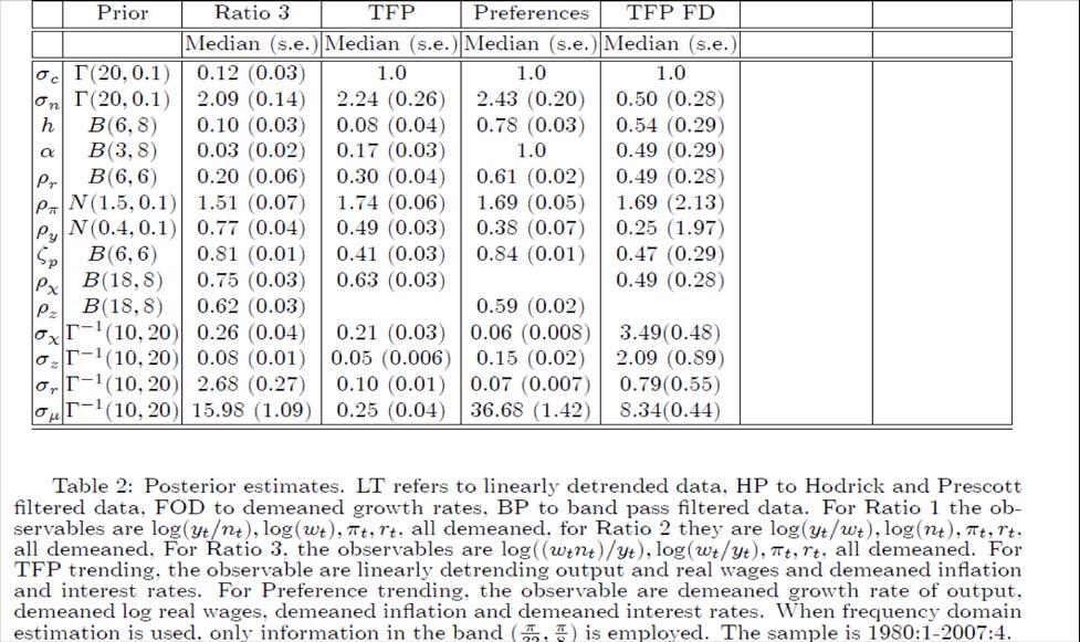
79 LT FOD Flexible Output Inflation Output Inflation Output Inflation TFP shocks Gov. expenditure shocks Investment shocks Monetary policy shocks Price markup shocks.75(*).88(*).91(*).9(*)..21 Wage markup shocks (*) Preference shocks (*). Variance decomposition at the 5 years horizon, SW model. Estimates are obtained using the median of the posterior of the parameters. A (*) indicates that the 68 percent highest credible set is entirely above.1. The model and the data set are the same as in Smets Wouters (27). LT refers to linearly detrended data, FOD to growth rates and Flexible to the approach this paper suggests.

80 5 Eliciting Priors from existing information - Prior distributions for DSGE parameters often arbitrary. - Prior distribution for individual parameters assumed to be independent: the joint distribution may assign non-zero probability to unreasonable regions of the parameter space. - Prior sometimes set having some statistics in mind (the prior mean is similar to the one obtained in calibration exercises). - Same prior is used for the parameters of different models. Problem: same prior may generate very different dynamics in different models. Hard to compare the outputs.

81 Example 5.1 Let = ( 1). Suppose 1 and 2 are independent and ( 1 ) ( 1 ) ; ( 2 1 ) ( ). Since the mean of is = 2 1 1,thepriorfor 1 and 2 imply that 1 ( (1 1 ). ) 2 Hence, the prior mean of has a variance which is increasing in the persistence parameter 1! Why? Reasonable? Alternative: state a prior for, derive the prior for 1 and 2 (change of variables). For example, if ( 2 ) then ( 1 )= ( 1 ) ( 2 1 )= ( (1 1 ) 2 (1 1 ) 2 ). Note here that the priors for 1 and 2 are correlated. Suppose you want to compare the model with = + ( 1). If ( ) = ( 2 ) the two models are immediately comparable. If, instead, we had assumed independent priors for ( 1 ) and ( 2 ), the two models would not be comparable (standard prior has weird predictions for the prior of the mean of ).

82 - Del Negro and Schorfheide (28): elicit priors consistent with some distribution of statistics of actual data (see also Kadane et al. (198)). Basic idea: i) Let be a set of DSGE parameters. Let be a set of statistics obtained in the data with observations and be the standard deviation of these statistics (which can be computed using asymptotic distributions or small sample devices, such as bootstrap or MC methods). ii) Let ( ) be the same set of statistics which are measurable from the model once is selected using observations. Then = ( )+ ( Σ ) (42) where is a set of measurement errors.

83 Note i) in calibration exercises Σ =and are averages of the data. ii) in SMM: Σ =and are generic moments of the data. Then ( ( ) )= ( ( )), where the latter is the conditional density in (42). Given any other prior information ( ) (whichisnotbasedon )the prior for is ( ) ( ( ) ) ( ) (43)

84 - ( ) ( ): overidentification is possible. -EvenifΣ is diagonal, ( ) will induce correlation across. -Information used to construct should be different than information used to estimate the model. Could be data in a training sample or could be data from a different country or a different regime (see e.g. Canova and Pappa, 27). - Assume that are normal why? Make life easy, Could also use other distributions, e.g. uniform, t. -Whatarethe? Could be steady states, autocorrelation functions, etc. What is depends on where the parameters enters.

85 Example 5.2 max ( +1 ) X ( (1 ) 1 ) 1 1 (44) = +(1 ) (45) ln = + ln ( 2 ) (46) ln = + ln ( 2 ) (47) = 1 (48) are given, is consumption, is hours, is the capital stock. Let be financed with lump sum taxes and thelagrangianon(45).

86 The FOC are ((52) and (53) equate factor prices and marginal products) = (1 ) 1 (1 ) (1 )(1 ) (49) 1 1 = (1 ) (1 ) (1 ) (1 )(1 ) 1 (5) = +1 [(1 ) (1 )] (51) = (52) = (1 ) (53) Using (49)-(5) we have: 1 1 = (54)

87 Log linearizing the equilibrium conditions ˆ ( (1 ) 1)ˆ +(1 )(1 ) 1 ˆ = (55) (1 )( ) ˆ +1 + (1 )( ) +(1 )) ( \ +1 ˆ +1 ) = ˆ (56) 1 1 ˆ +ˆ d = (57) ˆ \ +ˆ = (58) ˆ \ + ˆ = (59) \ ˆ (1 ) ˆ ˆ = (6) ( ) ˆ +( ) ˆ +( ) ( ˆ +1 (1 ) ˆ ) \ = (61) (6) and (61) are the production function and resource constraint.

88 Four types of parameters appear in the log-linearized conditions: i.) Technological parameters ( ). ii) Preference parameters ( ). iii) Steady state parameters ( ( ) ( ) ( iv) Parameters of the driving process ( 2 2 ). Question: How do we set a prior for these 13 parameters? ) ).

89 The steady state of the model (using (51)-(54)-(45)) is: 1 ( ) = 1 (62) [(1 )( ) +(1 )] = 1 (63) ( ) +( ) + ( ) = 1 (64) = (65) = (66) Five equations in 8 parameters!! Need to choose. For example: (62)-(66) determine ( ( ) ( ) ) given (( ), ).

90 Set 2 =[( ), ] and 1 =[ ( ) ( ) ] Then if 1 are steady state relationships, we an use (62)-(66) to construct a prior distribution for 1 2. How do we measure uncertainty in 1? - Take a rolling window to estimate 1 and use uncertainty of the estimate to calibrate var( ). - Bootstrap 1,etc.

91 Howdowesetapriorfor 2? Use additional information (statistics)! - ( ) couldbecenteredattheaverageg/yinthedatawithstandard error covering the existing range of variations - =(1+ ) 1 and typically =[ 75 15] per quarter. Choose a prior centered at around those values and e.g. uniformly distributed. - is related to Frish elasticity of labor supply: use estimates of labor supply elasticity to obtain histograms and to select a prior shape. Note: uncertainty in this case could be data based or across studies (meta uncertainty).

92 Parameters of the driving process ( 2 2 ) do not enter the steady state. Call them 3. How do we choose a prior for them? - 2 can be backed out from moments of Solow residual i.e. estimate the variance and the AR(1) of ˆ =ln (1 ),once is chosen. Prior for induce a distribution for ˆ - 2 backed out from moments government expenditure data. Prior standard errors should reflect variations in the data of these parameters.

93 -For (coefficient of relative risk aversion (RRA) is 1 (1 )) one has two options: (a) appeal to existing estimates of RRA. Construct a prior which is consistent with the cross section of estimates (e.g. a 2 (2) would be ok). (b) select an interesting moment, say ( ) and use ( )= ( ( ) )+ (67) to back out a prior for.

94 For some parameters (call them 5 ) we have no moments to match but some micro evidence. Then ( 5 )= ( 5 ) could be estimated from the histogram of the estimates which are available. In sum, the prior for the parameters is ( ) = ( 1 1 ) ( 2 2 ) ( 3 3 ) ( 4 4 ) ( 1 ) ( 2 ) ( 3 ) ( 4 )Π( 5 ) (68)

95 -Ifwehadusedadifferent utility function, the prior e.g. for 1 4 would be different. Prior for different models/parameterizations should be different. - To use these priors, need a normalizing constant ( (43 is not necessarily a density). Need a RW metropolis to draw from the priors we have produced. - Careful about multidimensional ridges: e.g. steady states are 5 equations, and there are 8 parameters - solution not unique, impossible to invert the relationship. -Carefulaboutchoosing 3 and 4 when there are weak and partial identification problems.

96 Extension: Lombardi and Nicoletti (211) Employ user-supplied impulse response to get a joint prior for the parameters - user supplied vector of IRF; ( ) modelbasedirf. - Distance function ( )= ( ( ) ) ( ( ) ), weighting matrix. - Prior kernel: ( )= ( ( )) (1+ ( ( )) -Prior: ( )= ( ) R ( ).

97 =[ 1 2 ]. Two special cases: 1) Prior kernel ( 1 2 ) (some parameters do not enter impulse responses and are calibrated). 2) Prior kernel ( 1 2 ) ( 2 2 Σ 2 ) (prior for some parameters obtained from sources other than IRF).

98 6 Non linear DSGE models 2 +1 = 1 ( 2 1 ) (69) 1 = 2 ( 2 2 ) (7) 2 = measurement errors, 1 = structural shocks, = vector of structural parameters, 2 = vector of states, 1 = vector of controls. Let = ( 1 2 ), =( 1 2 ), 1 =( 1 )and =( 1 ). Likelihood is L( 2 )= Q =1 ( 1 ) ( 2 ). Integrating the initial conditions 2 and the shocks out, we have: L( )= Z [ Y Z =1 (71) is intractable. ( 1 2 ) ( 1 2 ) ] ( 2 ) 2 (71)

99 If we have draws for 2 from ( 2 ) and draws for 1, =1 =1,from ( 1 2 ) approximate (71) with L( )= 1 [ Y =1 1 X ( )] (72) Drawing from ( 2 ) is simple; drawing from ( 1 2 )complicated. Fernandez Villaverde and Rubio Ramirez (24): use ( ) as importance sampling for ( 1 2 ):

100 -Draw 2 from ( 2 ). Draw 1 times from ( 1 2 )= ( ) ( ). -Construct = 1. ( P ) =1 ( and assign it to each draw ) -Resamplefrom{ 1 } =1 with probabilities equal to. - Repeat above steps for every =1 2. Step 3) is crucial, if omitted, only one particle will asymptotically remain and the integral in (71) diverges as. Algorithm is computationally demanding. You need a MC within a MC. Fernandez Villaverde and Rubio Ramirez (24): some improvements over linear specifications.