Seismic imaging and multiple removal via model order reduction

Transcription

1 Seismic imaging and multiple removal via model order reduction Alexander V. Mamonov 1, Liliana Borcea 2, Vladimir Druskin 3, and Mikhail Zaslavsky 3 1 University of Houston, 2 University of Michigan Ann Arbor, 3 Schlumberger-Doll Research Center Support: NSF DMS , ONR N A.V. Mamonov ROMs for imaging and multiple removal 1 / 26

2 Motivation: seismic oil and gas exploration Problems addressed: 1 Imaging: qualitative estimation of reflectors on top of known velocity model 2 Multiple removal: from measured data produce a new data set with only primary reflection events Common framework: data-driven Reduced Order Models (ROM) A.V. Mamonov ROMs for imaging and multiple removal 2 / 26

3 Forward model: acoustic wave equation Acoustic wave equation in the time domain with initial conditions u tt = Au in Ω, t [0, T ] u t=0 = B, u t t=0 = 0, sources are columns of B R N m The spatial operator A R N N is a (symmetrized) fine grid discretization of A = c 2 with appropriate boundary conditions Wavefields for all sources are columns of u(t) = cos(t A)B R N m A.V. Mamonov ROMs for imaging and multiple removal 3 / 26

4 Data model and problem formulations For simplicity assume that sources and receivers are collocated, receiver matrix is also B The data model is D(t) = B T u(t) = B T cos(t A)B, an m m matrix function of time Problem formulations: 1 Imaging: given D(t) estimate reflectors, i.e. discontinuities of c 2 Multiple removal: given D(t) obtain Born data set F(t) with multiple reflection events removed In both cases we are provided with a kinematic model, a smooth non-reflective velocity c 0 A.V. Mamonov ROMs for imaging and multiple removal 4 / 26

5 Reduced order models Data is always discretely sampled, say uniformly at t k = kτ The choice of τ is very important, optimally τ around Nyquist rate Discrete data samples are D k = D(kτ) = B T cos ( kτ ) A B = B T T k (P)B, where T k is Chebyshev polynomial and the propagator (Green s function over small time τ) is ( P = cos τ ) A R N N A reduced order model (ROM) P R mn mn, B R mn m should fit the data D k = B T T k (P)B = B T T k ( P) B, k = 0, 1,..., 2n 1 A.V. Mamonov ROMs for imaging and multiple removal 5 / 26

6 Projection ROMs Projection ROMs are of the form P = V T PV, B = V T B, where V is an orthonormal basis for some subspace What subspace to project on to fit the data? Consider a matrix of wavefield snapshots U = [u 0, u 1,..., u n 1 ] R N mn, u k = u(kτ) = T k (P)B We must project on Krylov subspace K n (P, B) = colspan[b, PB,..., P n 1 B] = colspan U Reasoning: the data only knows about what P does to wavefield snapshots u k A.V. Mamonov ROMs for imaging and multiple removal 6 / 26

7 ROM from measured data Wavefields in the whole domain U are unknown, thus V is unknown How to obtain ROM from just the data D k? Data does not give us U, but it gives us inner products! Multiplicative property of Chebyshev polynomials T i (x)t j (x) = 1 2 (T i+j(x) + T i j (x)) Since u k = T k (P)B and D k = B T T k (P)B we get (U T U) i,j = u T i u j = 1 2 (D i+j + D i j ), (U T PU) i,j = u T i Pu j = 1 4 (D j+i+1 + D j i+1 + D j+i 1 + D j i 1 ) A.V. Mamonov ROMs for imaging and multiple removal 7 / 26

8 ROM from measured data Suppose U is orthogonalized by a block QR (Gram-Schmidt) procedure U = VL T, equivalently V = UL T, where L is a block Cholesky factor of the Gramian U T U known from the data U T U = LL T The projection is given by P ( ) = V T PV = L 1 U T PU L T, where U T PU is also known from the data Cholesky factorization is essential, (block) lower triangular structure is the linear algebraic equivalent of causality A.V. Mamonov ROMs for imaging and multiple removal 8 / 26

9 Problem 1: Imaging ROM is a projection, we can use backprojection If span(u) is suffiently rich, then columns of VV T should be good approximations of δ-functions, hence P VV T PVV T = V PV T As before, U and V are unknown We have an approximate kinematic model, i.e. the travel times Equivalent to knowing a smooth velocity c 0 For known c 0 we can compute everything, including U 0, V 0, P0 A.V. Mamonov ROMs for imaging and multiple removal 9 / 26

10 ROM backprojection Take backprojection P V PV T and make another approximation: replace unknown V with V 0 P V0 PV T For the kinematic model we know V 0 exactly 0 P 0 V 0 P0 V T 0 Approximate perturbation of the propagator P P 0 V 0 ( P P 0 )V T 0 is essentially the perturbation of the Green s function δg(x, y) = G(x, y, τ) G 0 (x, y, τ) But δg(x, y) depends on two variables x, y Ω, how do we get a single image? A.V. Mamonov ROMs for imaging and multiple removal 10 / 26

11 Backprojection imaging functional Take the imaging functional I to be I(x) δg(x, x) = G(x, x, τ) G 0 (x, x, τ), x Ω In matrix form it means taking the diagonal ( I = diag V 0 ( P P ) 0 )V T 0 diag(p P 0 ) Note that ) I = diag ([V 0 V T ] P [VV T 0 ] [V 0V T 0 ] P 0 [V 0 V T 0 ] Thus, approximation quality depends only on how well columns of VV T 0 and V 0V T 0 approximate δ-functions A.V. Mamonov ROMs for imaging and multiple removal 11 / 26

12 Simple example: layered model True c ROM backprojection image I A simple layered model, p = 32 sources/receivers (black ) Constant velocity kinematic model c 0 = 1500 m/s Multiple reflections from waves bouncing between layers and reflective top surface Each multiple creates an RTM artifact below actual layers RTM image A.V. Mamonov ROMs for imaging and multiple removal 12 / 26

13 Snapshot orthogonalization Snapshots U Orthogonalized snapshots V t = 10τ t = 15τ t = 20τ A.V. Mamonov ROMs for imaging and multiple removal 13 / 26

14 Snapshot orthogonalization Snapshots U Orthogonalized snapshots V t = 25τ t = 30τ t = 35τ A.V. Mamonov ROMs for imaging and multiple removal 14 / 26

15 Approximation of δ-functions Columns of V0 VT0 Columns of VVT0 y = 345 m y = 510 m y = 675 m A.V. Mamonov ROMs for imaging and multiple removal 15 / 26

16 Approximation of δ-functions Columns of V0 VT0 Columns of VVT0 y = 840 m y = 1020 m y = 1185 m A.V. Mamonov ROMs for imaging and multiple removal 16 / 26

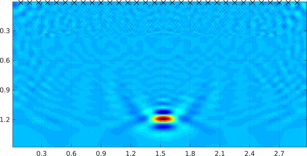
17 High contrast example: hydraulic fractures True c RTM image Important application: hydraulic fracturing Three fractures 10 cm wide each Very high contrasts: c = 4500 m/s in the surrounding rock, c = 1500 m/s in the fluid inside fractures A.V. Mamonov ROMs for imaging and multiple removal 17 / 26

18 High contrast example: hydraulic fractures True c ROM backprojection image I Important application: hydraulic fracturing Three fractures 10 cm wide each Very high contrasts: c = 4500 m/s in the surrounding rock, c = 1500 m/s in the fluid inside fractures A.V. Mamonov ROMs for imaging and multiple removal 18 / 26

19 Large scale example: Marmousi model A.V. Mamonov ROMs for imaging and multiple removal 19 / 26

20 Problem 2: multiple removal Introduce Data-to-Born (DtB) transform: compute ROM from original data, then generate a new data set with primary reflection events only Born with respect to what? Consider wave equation in the form ( c ) u tt = σc σ u, where acoustic impedance σ = ρc Assume c = c 0 is a known kinematic model Only the impedance σ changes Above assumptions are for derivation only, the method works even if they are not satisfied A.V. Mamonov ROMs for imaging and multiple removal 20 / 26

21 Born approximation Can show that where P I τ 2 L q = c c q, 2 L ql T q, LT q = c c q, are affine in q = log σ Consider Born approximation (linearization) with respect to q around known c = c 0 Perform second Cholesky factorization on ROM 2 τ 2 (Ĩ P) = L q LT q Cholesky factors L q, L T q are approximately affine in q, thus the perturbation L q L 0 is approximately linear in q A.V. Mamonov ROMs for imaging and multiple removal 21 / 26

22 Data-to-Born transform 1 Compute P from D and P 0 from D 0 corresponding to q 0 (σ 1) 2 Perform second Cholesky factorization, find L q and L 0 3 Form the perturbation L ε = L 0 + ε( L q L 0 ), affine in εq 4 Propagate the perturbation ( D ε k = B T T k Ĩ τ 2 ) 2 L ε LT ε B 5 Differentiate to obtain DtB transformed data F k = D 0 k + ddε k dε, k = 0, 1,..., 2n 1 ε=0 A.V. Mamonov ROMs for imaging and multiple removal 22 / 26

23 Example: DtB seismogram comparison Impedance σ = ρc Velocity c Original data D k D 0 k DtB transformed data F k D 0 k A.V. Mamonov ROMs for imaging and multiple removal 23 / 26

24 Example: DtB+RTM imaging Impedance σ = ρc Velocity c RTM image from original data RTM image from DtB data A.V. Mamonov ROMs for imaging and multiple removal 24 / 26

25 Conclusions and future work ROMs for imaging and multiple removal (DtB) Time domain formulation is essential, linear algebraic analogues of causality: Gram-Schmidt, Cholesky Implicit orthogonalization of wavefield snapshots: removal of multiples in backprojection imaging and DtB transform Existing linearized imaging (RTM) and inversion (LS-RTM) methods can be applied to DtB transformed data Future work: Data completion for partial data (including monostatic, aka backscattering measurements) Elasticity: promising preliminary results Stability and noise effects (SVD truncation of the Gramian, etc.) Frequency domain analogue (data-driven PML) A.V. Mamonov ROMs for imaging and multiple removal 25 / 26

26 References 1 Nonlinear seismic imaging via reduced order model backprojection, A.V. Mamonov, V. Druskin, M. Zaslavsky, SEG Technical Program Expanded Abstracts 2015: pp Direct, nonlinear inversion algorithm for hyperbolic problems via projection-based model reduction, V. Druskin, A. Mamonov, A.E. Thaler and M. Zaslavsky, SIAM Journal on Imaging Sciences 9(2): , A nonlinear method for imaging with acoustic waves via reduced order model backprojection, V. Druskin, A.V. Mamonov, M. Zaslavsky, 2017, arxiv: [math.na] 4 Untangling the nonlinearity in inverse scattering with data-driven reduced order models, L. Borcea, V. Druskin, A.V. Mamonov, M. Zaslavsky, 2017, arxiv: [math.na] A.V. Mamonov ROMs for imaging and multiple removal 26 / 26