The Singular-Value Decomposition

Transcription

1 Mathematical Tools for Data Science Spring Motivation The Singular-Value Decomposition The singular-value decomposition (SVD) is a fundamental tool in linear algebra. In this section, we introduce three data-science applications where the SVD plays a crucial role. 1.1 Dimensionality reduction Consider a set of data each consisting of several features. It is often useful to model such data as a set of vectors in a multidimensional space where each dimension corresponds to a feature. The dataset can then be viewed as a cloud of points or if we prefer a probabilistic perspective as a probability density in R p, where p is the number of features. A natural question is in what directions of R p the dataset has more or less variation. In directions where there is little or no variation, the properties of the dataset are essentially constant, so we can safely ignore them. This is very useful when the number of features p is large; the remaining directions form a space of reduced dimensionality, which reduces the computational cost of the analysis. Dimensionality reduction is a crucial preprocessing step in big-data applications. The SVD provides a complete characterization of the variance of a p-dimensional dataset in every direction of R p, and is therefore very useful for this purpose. 1.2 Linear regression Regression is a fundamental problem in statistics. The goal is to estimate a quantity of interest called the response or the dependent variable, from the values of several observed variables known as covariates, features or independent variables. For example, if the response is the price of a house, the covariates can be its size, the number of rooms, the year it was built, etc. A regression model produces an estimate of the house prices as a function of all of these factors. More formally, let the response be denoted by a scalar y R and the features by a vector x R p (p is the number of features). The goal is to construct a function h that maps x to y, i.e. such that y h ( x), (1) from a set of examples, called a training set. corresponding features This set contains specific responses and their S train := {( y (1), x (1)), ( y (2), x (2)),..., ( y (n), x (n))}. (2) An immediate complication is that there exist infinite possible functions mapping the features to the right response with no error in the training set (as long as all the feature vectors are distinct). 1

2 74 72 Height (inches) Linear regression model Weight (pounds) Figure 1: The image shows a linear regression model (red line) of the height of a population of 25,000 people given their weight, superposed on a scatter plot of the actual data (in blue). The data are available here. It is crucial to constrain h so that it generalizes to new examples. A very popular choice is to assume that the regression function is linear, so that y x, β + β 0 (3) for a vector of linear coefficients β R p and a constant β 0 R (strictly speaking the function is affine). Figure 1 shows an example, where the response is the height of a person and the only covariate is their weight. We will study the generalization properties of linear-regression models using the SVD. 1.3 Bilinear model for collaborative filtering Collaborative filtering is the problem of predicting the interests of users from data. Figure 2 shows an example where the goal is to predict movie ratings. Assume that y[i, j] represents the rating assigned to a movie i by a user j. If we have available a dataset of such ratings, how can we estimate the rating corresponding to a tuple (i, j) that we have not seen before? A reasonable assumption is that some movies are more popular than others, and some users are more generous than others. Let a[i] quantify the popularity of movie i and b[j] the generosity of user j. A large value of a[i] indicates that i is very popular, a large value of b[j] indicates that j is very generous. If we are able to estimate these quantities from data, then a reasonable estimate for the rating given by user j to movie i is given by y[i, j] a[i]b[j]. (4) The model in Eq. (4) is extremely simplistic: different people like different movies! In order to generalize it we can consider r factors that capture the dependence between the ratings and the 2

3 ??????????????? Figure 2: A depiction of the collaborative-filtering problem as an incomplete ratings matrix. Each row corresponds to a user and each column corresponds to a movie. The goal is to estimate the missing ratings. The figure is due to Mahdi Soltanolkotabi. movie/user y[i, j] r a l [i]b l [j]. (5) l=1 Each user and each movie is now described by r features each, with the following interpretation: a l [i]: movie i is positively (> 0), negatively (< 0) or not ( 0) associated to factor l. b l [j]: user j is positively (> 0), negatively (< 0) or not ( 0) associated to factor l. The model is not linearly dependent on the features. Instead, it is bilinear. If the movie features are fixed, the model is linear in the user features; if the user features are fixed, the model is linear in the movie features. As we shall see, the SVD can be used to fit bilinear models. 2 Singular-value decomposition 2.1 Definition Every real matrix has a singular-value decomposition (SVD). 3

4 Theorem 2.1. Every rank r real matrix A R m n, has a singular-value decomposition (SVD) of the form s v 1 T A = [ ] 0 s 2 0 v T u 1 u 2 u r... (6) s r = USV T, (7) where the singular values s 1 s 2 s r are positive real numbers, the left singular vectors u 1, u 2,... u r form an orthonormal set, and the right singular vectors v 1, v 2,... v r also form an orthonormal set. The SVD is unique if all the singular values are different. If several singular values are the same, the corresponding left singular vectors can be replaced by any orthonormal basis of their span, and the same holds for the right singular vectors. The SVD of an m n matrix with m n can be computed in O (mn 2 ). We refer to any graduate linear algebra book for the proof of Theorem 2.1 and for details on how to compute the SVD. The SVD provides orthonormal bases for the column and row spaces of a matrix. Lemma 2.2. The left singular vectors are an orthonormal basis for the column space, whereas the right singular vectors are an orthonormal basis for the row space. Proof. We prove the statement for the column space, the proof for the row space is identical. All left singular vectors belong to the column space because u i = A ( ) s 1 i v i. In addition, every column of A is in their span because A :i = U ( ) SV T e i. Since they form an orthonormal set by Theorem 2.1, this completes the proof. The SVD presented in Theorem 2.1 can be augmented so that the number of singular values equals min (m, n). The additional singular values are all equal to zero. Their corresponding left and right singular vectors are orthonormal sets of vectors in the orthogonal complements of the column and row space respectively. If the matrix is tall or square, the additional right singular vectors are a basis of the null space of the matrix. Corollary 2.3 (Singular-value decomposition). Every rank r real matrix A R m n, where m n, has a singular-value decomposition (SVD) of the form s s A := [ u 1 u 2 u }{{} r u r+1 u n ] 0 0 s r 0 0 [ v 1 v 2 v r v Basis of range(a) }{{} r+1 v n ] T, (8) }{{} Basis of row(a) Basis of null(a) where the singular values s 1 s 2 s r are positive real numbers, the left singular vectors u 1, u 2,..., u m form an orthonormal set in R m, and the right singular vectors v 1, v 2,..., v m form an orthonormal basis for R n. v T r 4

5 If the matrix is fat, we can define a similar augmentation, where the additional left singular vectors form an orthonormal basis of the orthogonal complement of the range. 2.2 Geometric interpretation The SVD decomposes the action of a matrix A R m n on a vector x R n into three simple steps, illustrated in Figure 3: 1. Rotation of x to align the component of x in the direction of the ith right singular vector v i with the ith axis: V T x = v i, x e i. (9) 2. Scaling of each axis by the corresponding singular value SV T x = s i v i, x e i. (10) 3. Rotation to align the ith axis with the ith left singular vector USV T x = s i v i, x u i. (11) This geometric perspective of the SVD reveals an important property: the maximum scaling produced by a matrix is equal to the maximum singular value. The maximum is achieved when the matrix is applied to any vector in the direction of the right singular vector v 1. If we restrict our attention to the orthogonal complement of v 1, then the maximum scaling is the second singular value, due to the orthogonality of the singular vectors. In general, the direction of maximum scaling orthogonal to the first i 1 left singular vectors is equal to the ith singular value and occurs in the direction of the ith singular vector. Theorem 2.4. For any matrix A R m n, with SVD given by (8), the singular values satisfy s 1 = s i = the right singular vectors satisfy max A x { x 2 =1 x R n 2 (12) } = max { y 2 =1 y R m } AT y 2, (13) max A x 2, (14) { x 2 =1 x R n, x v 1,..., v i 1 } = max A T y 2, 2 i min {m, n}, (15) { y 2 =1 y R m, y u 1,..., u i 1 } v 1 = v i = arg max A x 2, (16) { x 2 =1 x R n } arg max A x 2, 2 i m, (17) { x 2 =1 x R n, x v 1,..., v i 1 } 5

6 (a) s 1 = 3, s 2 = 1. x v 2 V T x e 2 V T y y V T e 1 v 1 S SV T x s 2 e 2 SV T y U s2 u 2 USV T y s 1 u 1 s 1 e 1 USV T x (b) s 1 = 3, s 2 = 0. x v 2 V T x e 2 V T y y V T e 1 v 1 S USV T y s 1 u 1 SV T x 0 SV T y s 1 e 1 U 0 USV T x Figure 3: The action of any matrix can be decomposed into three steps: rotation to align the right singular vectors to the axes, scaling by the singular values and a final rotation to align the axes with the left singular vectors. In image (b) the second singular value is zero, so the matrix projects two-dimensional vectors onto a one-dimensional subspace. 6

7 and the left singular vectors satisfy u 1 = u i = arg max A T y 2, (18) { y 2 =1 y R m } arg max A T y 2, 2 i n. (19) { y 2 =1 y R m, y u 1,..., u i 1 } Proof. Consider a vector x R n with unit l 2 norm that is orthogonal to v 1,..., v i 1, where 1 i n (if i = 1 then x is just an arbitrary vector). We express x in terms of the right singular vectors of A and a component that is orthogonal to their span x = α j v j + P row(a) x (20) j=i where 1 = x 2 2 n j=i α2 j. By the ordering of the singular values in Theorem 2.1 A x 2 2 = = = = s 2 i s k v k, x u k, k=1 s k v k, x u k by (11) (21) k=1 s 2 k v k, x 2 because u 1,..., u n are orthonormal (22) k=1 s 2 k v k, k=1 α j v j + P row(a) x 2 (23) j=i s 2 jαj 2 because v 1,..., v n are orthonormal (24) j=i αj 2 because s i s i+1... s n (25) j=i s 2 i by (20). (26) This establishes (12) and (14). To prove (16) and (17) we show that v i achieves the maximum A v i 2 2 = s 2 k v k, v i 2 (27) k=1 = s 2 i. (28) The same argument applied to A T establishes (13), (18), (19) and (15). 3 Principal component analysis 3.1 Quantifying directional variation In this section we describe how to quantify the variation of a dataset embedded in a p-dimensional space. We can take two different perspectives: 7

8 Probabilistic: The data are samples from a p-dimensional random vector x characterized by its probability distribution. Geometric: The data are just a just a cloud of points in R p. Both perspectives are intertwined. Let us first consider a set of scalar values {x 1, x 2,..., x n }. If we interpret them as samples from a random variable x, then we can quantify their average variation using the variance of x, defined as the expected value of its squared deviation from the mean, Var (x) := E ( (x E (x)) 2). (29) Recall that the square root of the variance is known as the standard deviation of the random variable. If we prefer a geometric perspective we can instead consider the average of the squared deviation of each point from their average var (x 1, x 2,..., x n ) := 1 (x i av (x 1, x 2,..., x n )) 2, n 1 (30) av (x 1, x 2,..., x n ) := 1 x i. n (31) This quantity is the sample variance of the points, which can be interpreted as an estimate of their variance if they are generated from the same probability distribution. Similarly, the average is the sample mean, and can be interpreted as an estimate of the mean. More formally, let us consider a set of random variables {x 1, x 2,..., x n } with the same mean µ and variance σ 2. We have E (av (x 1, x 2,..., x n )) = µ, (32) E (var (x 1, x 2,..., x n )) = σ 2, (33) by linearity of expectation. In statistics jargon, the sample mean and variance are unbiased estimators of the true mean and variance. In addition, if the variables are independent, by linearity of expectation, E ( (av (x 1, x 2,..., x n ) µ) 2) = σ2 n. (34) Furthermore, if the fourth moment of the random( variables x 1, x 2,..., x n is bounded (i.e. there is some constant c such that E (x 4 i ) c for all i), E (var (x 1, x 2,..., x n ) σ 2 ) 2) also scales as 1/n. In words, the mean square error incurred by the estimators decreases linearly with the number of data. When the number of data is large, the probabilistic and geometric viewpoints are essentially equivalent, although it is worth emphasizing that the geometric perspective is still relevant if we want to avoid making probabilistic assumptions. In order to extend the notion of average variation to a multidimensional dataset, we first need to center the data. This can be done by subtracting their average. Then we can consider the projection of the data onto any direction of interest, by computing the inner product of each centered data point with the corresponding unit-norm vector v R p. If we take a probabilistic 8

9 perspective, where the data are samples of a p-dimensional random vector x, the variation in that direction is given by the variance of the projection Var ( v T x ). This variance can be estimated using the sample variance var ( v T x 1, v T x 2,..., v T x n ), where x1,..., x n R p are the actual data. This has a geometric interpretation in its own right, as the average square deviation of the projected data from their average. 3.2 Covariance matrix In this section we show that the covariance matrix captures the average variation of a dataset in any direction. The covariance of two random variables x and y provides an average of their joint fluctuations around their respective means, Cov (x, y) := E ((x E (x)) (y E (y))). (35) The covariance matrix of a random vector contains the variance of each component in the diagonal and the pairwise covariances between different components in the off diagonals. Definition 3.1. The covariance matrix of a random vector x is defined as Var ( x [1]) Cov ( x [1], x [2]) Cov ( x [1], x [p]) Cov ( x [2], x [1]) Var ( x [2]) Cov ( x [2], x [p]) Σ x := Cov ( x [n], x [1]) Cov ( x [n], x [2]) Var ( x [p]) (36) = E ( x x T ) E( x)e( x) T. (37) Note that if all the entries of a vector are uncorrelated, then its covariance matrix is diagonal. Using linearity of expectation, we obtain a simple expression for the covariance matrix of the linear transformation of a random vector. Theorem 3.2 (Covariance matrix after a linear transformation). Let x be a random vector of dimension n with covariance matrix Σ. For any matrix A R m p, Proof. By linearity of expectation Σ A x = E Σ A x = AΣ x A T. (38) ( (A x) (A x) T ) E (A x) E (A x) T (39) = A ( E ( x x T ) E( x)e( x) T ) A T (40) = AΣ x A T. (41) An immediate corollary of this result is that we can easily decode the variance of the random vector in any direction from the covariance matrix. 9

10 Corollary 3.3. Let v be a unit-l 2 -norm vector, Var ( v T x ) = v T Σ x v. (42) The variance of a random variable cannot be negative by definition (it is the expectation of a nonnegative quantity). The corollary therefore implies that covariance matrices are positive semidefinite, i.e. for any Σ x and any vector v, v T Σ x v 0. Symmetric, positive semidefinite matrices have the same left and right singular vectors 1. The SVD of the covariance matrix of a random vector x is therefore of the form Σ x = USU T (43) s = [ ] u 1 u 2 u n 0 s 2 0 [ ] T u1 u 2 u n. (44) 0 0 s n The SVD of the covariance matrix provides very valuable information about the directional variance of the random vector. Theorem 3.4. Let x be a random vector of dimension p with covariance matrix Σ x. The SVD of Σ x given by (44) satisfies for 2 k p. s 1 = max v 2 =1 Var ( v T x ), (45) u 1 = arg max v 2 =1 Var ( v T x ), (46) s k = Proof. By Corollary 3.3, the directional variance equals max v 2 =1, v u 1,..., u k 1 Var ( v T x ), (47) u k = arg max Var ( v T x ), (48) v 2 =1, v u 1,..., u k 1 v T Σ x v = v T USU T v (49) = SU T v, (50) where S is a diagonal matrix that contains the square root of the entries of S. The result then follows from Theorem 2.4 since SU T is a valid SVD. In words, u 1 is the direction of maximum variance. The second singular vector u 2 is the direction of maximum variation that is orthogonal to u 1. In general, the eigenvector u k reveals the direction of maximum variation that is orthogonal to u 1, u 2,..., u k 1. Finally, u p is the direction of minimum variance. Figure 4 illustrates this with an example, where p = 2. 1 If a matrix is symmetric but not positive semidefinite, some right singular vectors v j may equal u j instead of u j

11 s1 = 1.22, s 2 = 0.71 s1 = 1, s 2 = 1 s1 = 1.38, s 2 = 0.32 Figure 4: Samples from bivariate Gaussian random vectors with different covariance matrices are shown in gray. The eigenvectors of the covariance matrices are plotted in red. Each is scaled by the square roof of the corresponding singular value s 1 or s Sample covariance matrix A natural estimator of the covariance matrix is the sample covariance matrix. Definition 3.5 (Sample covariance matrix). Let { x 1, x 2,..., x n } be a set of m-dimensional realvalued data vectors, where each dimension corresponds to a different feature. The sample covariance matrix of these vectors is the p p matrix Σ ( x 1,..., x n ) := 1 n 1 ( x i av ( x 1,..., x n )) ( x i av ( x 1,..., x n )) T, (51) where the center or average is defined as av ( x 1, x 2,..., x n ) := 1 n x i (52) contains the sample mean of each feature. The (i, j) entry of the covariance matrix, where 1 i, j p, is given by { var ( x 1 [i],..., x n [i]) if i = j, Σ ( x 1,..., x n ) ij = (53) cov (( x 1 [i], x 1 [j]),..., ( x n [i], x n [j])) if i j, where the sample covariance is defined as cov ((x 1, y 1 ),..., (x n, y n )) := 1 n 1 (x i av (x 1,..., x n )) (y i av (y 1,..., y n )). (54) By linearity of expectation, as sketched briefly in Section 3.1 the sample variance converges to the true variance if the data are independent (and the fourth moment is bounded). By the same argument, the sample covariance also converges to the true covariance under similar conditions. 11

12 n = 5 n = 20 n = 100 True covariance Sample covariance Figure 5: Singular vectors of the sample covariance matrix of n iid samples from a bivariate Gaussian distribution (red) compared to the singular vectors of its covariance matrix (black). As a result, the sample covariance matrix is often an accurate estimate of the covariance matrix, as long as enough samples are available. Figure 5 illustrates this with a numerical example, where the singular vectors of the sample covariance matrix converge to the singular vectors of the covariance matrix as the number of samples increases. Even if the data are not interpreted as samples from a distribution, the sample covariance matrix has an intuitive geometric interpretation. For any unit-norm vector v R p, the sample variance of the data set in the direction of v is given by var ( v T x 1,..., v T x n ) = 1 n 1 = 1 n 1 ( = v T ( v T x i av ( )) v T x 1,..., v T 2 x n (55) ( v T ( x i av ( x 1,..., x n )) ) 2 1 n 1 ) ( x i av ( x 1,..., x n )) ( x i av ( x 1,..., x n )) T v (56) = v T Σ ( x 1,..., x n ) v. (57) Using the sample covariance matrix we can extract the sample variance in every direction of the ambient space. 3.4 Principal component analysis The previous sections show that computing the SVD of the sample covariance matrix of a dataset reveals the variation of the data in different directions. This is known as principal-component analysis (PCA). Algorithm 3.6 (Principal component analysis). Given n data vectors x 1, x 2,..., x n R d, compute the SVD of the sample covariance of the data. The singular vectors are called the principal directions of the data. The principal components are the coefficients of the centered data vectors when expressed in the basis of principal directions. 12

13 s1 /(n 1) = 0.705, s2 /(n 1) = s1 /(n 1) = 0.983, s2 /(n 1) = s1 /(n 1) = 1.349, s2 /(n 1) = u 1 u 1 u 1 u 2 v Figure 6: PCA of a dataset with n = 100 2D vectors with different configurations. The two first singular values reflect how much energy is preserved by projecting onto the two first principal directions. u 2 u 2 An equivalent procedure to compute the principal directions is to center the data and then compute the SVD of the matrix c i = x i av ( x 1, x 2,..., x n ), 1 i n, (58) C = [ c 1 c 2 c n ]. (59) The result is the same because the sample covariance matrix is equal to 1 n 1 CCT. By Eq. (57) and Theorem 2.4 the principal directions reveal the directions of maximum variation of the data. Corollary 3.7. Let u 1,..., u k be the k min {p, n} first principal directions obtained by applying Algorithm 3.6 to a set of vectors x 1,..., x n R p. Then the principal directions satisfy u 1 = u i = and the associated singular values satisfy s 1 n 1 = s i n 1 = for any 2 k p. arg max var ( ) v T x 1,..., v T x n, (60) { v 2 =1 v R n } arg max var ( ) v T x 1,..., v T x n, 2 i k, (61) { v 2 =1 v R n, v u 1,..., u i 1 } max var ( ) v T x 1,..., v T x n, (62) { v 2 =1 v R n } max var ( ) v T x 1,..., v T x n, 2 i k (63) { v 2 =1 v R n, v u 1,..., u i 1 } In words, u 1 is the direction of maximum variation, u 2 is the direction of maximum variation orthogonal to u 1, and in general u k is the direction of maximum variation that is orthogonal to u 1, u 2,..., u k 1. Figure 6 shows the principal directions for several 2D examples. In the following example, we apply PCA to a set of images. 13

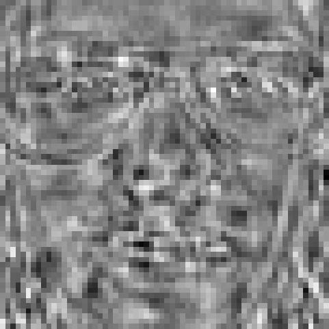
14 Center PD 1 PD 2 PD 3 PD 4 PD 5 si /(n 1) PD 10 PD 15 PD 20 PD 30 PD 40 PD PD 100 PD 150 PD 200 PD 250 PD 300 PD Figure 7: The top row shows the data corresponding to three different individuals in the Olivetti data set. The average and the principal directions (PD) obtained by applying PCA are depicted below. The corresponding singular value is listed below each principal direction. 14

15 Center PD 1 PD 2 PD 3 = PD 4 PD 5 PD 6 PD 7 Figure 8: Projection of one of the faces x onto the first 7 principal directions and the corresponding decomposition into the 7 first principal components. Signal 5 PDs 10 PDs 20 PDs 30 PDs 50 PDs 100 PDs 150 PDs 200 PDs 250 PDs 300 PDs 359 PDs Figure 9: Projection of a face on different numbers of principal directions. Example 3.8 (PCA of faces). In this example we consider the Olivetti Faces data set 2. The data set contains images taken from 40 different subjects (10 per subject). We vectorize each image so that each pixel is interpreted as a different feature. Figure 7 shows the center of the data and several principal directions, together with their associated singular values. The principal directions corresponding to the larger singular values seem to capture low-resolution structure, whereas the ones corresponding to the smallest singular values incorporate more intricate details. Figure 8 shows the projection of one of the faces onto the first 7 principal directions and the corresponding decomposition into its 7 first principal components. Figure 9 shows the projection of the same face onto increasing numbers of principal directions. As suggested by the visualization of the principal directions in Figure 7, the lower-dimensional projections produce blurry images. 2 Available at 15

16 3.5 Linear dimensionality reduction via PCA Data containing a large number of features can be costly to analyze. Dimensionality reduction is a useful preprocessing step, which consists of representing the data with a smaller number of variables. For data modeled as vectors in an ambient space R p (each dimension corresponds to a feature), this can be achieved by projecting the vectors onto a lower-dimensional space R k, where k < m. If the projection is orthogonal, the new representation can be computed using an orthogonal basis for the lower-dimensional subspace b 1, b 2,..., b k. Each data vector x R p is described using the coefficients of its representation in the basis: b 1, x, b 2, x,..., b k, x. Given a data set of n vectors x 1, x 2,..., x n R p, a crucial question is how to find the k- dimensional subspace that contains the most information. If we are interested in preserving the l 2 norm of the data, the answer is given by the SVD. If the data are centered, the best k-dimensional subspace is spanned by the first k principal directions. Theorem 3.9 (Optimal subspace for orthogonal projection). For any matrix with left singular vectors u 1,..., u n, we have A := [ a 1 a 2 a n ] R m n, (64) P span( u1, u 2,..., u k ) a i 2 2 P S a i 2 2, (65) for any subspace S of dimension k min {m, n}. Proof. Note that P span( u1, u 2,..., u k ) a i 2 2 = = k u j, a i 2 (66) j=1 k A T u j 2 2. (67) j=1 We prove the result by induction on k. The base case k = 1 follows immediately from (18). To complete the proof we show that if the result is true for k 1 1 (the induction hypothesis) then it also holds for k. Let S be an arbitrary subspace of dimension k. The intersection of S and the orthogonal complement to the span of u 1, u 2,..., u k 1 contains a nonzero vector b due to the following lemma. Lemma 3.10 (Proof in Section A). In a vector space of dimension n, the intersection of two subspaces with dimensions d 1 and d 2 such that d 1 + d 2 > n has dimension at least one. We choose an orthonormal basis b 1, b 2,..., b k for S such that b k := b is orthogonal to u 1, u 2,..., u k 1 16

17 30 Errors Number of principal components Figure 10: Errors for nearest-neighbor classification combined with PCA-based dimensionality reduction for different dimensions. (we can construct such a basis by Gram-Schmidt, starting with b). By the induction hypothesis, k 1 A T u i 2 2 = P span( u1, u 2,..., u k 1 ) a i 2 2 (68) P span( b 1, b 2,..., b k 1) a i 2 2 (69) k 1 = A T bi 2 2. (70) By (19) A T u k 2 2 A T bk 2 2. (71) Combining (70) and (71) we conclude P span( u1, u 2,..., u k ) a i 2 2 = = k A T u i 2 2 (72) k A T bi 2 2 (73) P S a i 2 2. (74) Example 3.11 (Nearest neighbors in principal-component space). The nearest-neighbor algorithm is a classical method to perform classification. Assume that we have access to a training 17

18 Test image Projection Closest projection Corresponding image Figure 11: Results of nearest-neighbor classification combined with PCA-based dimensionality reduction of order 41 for four of the people in Example The assignments of the first three examples are correct, but the fourth is wrong. 18

19 set of n pairs of data encoded as vectors in R p along with their corresponding labels: { x 1, l 1 },..., { x n, l n }. To classify a new data point y we find the closest element of the training set, i := arg min 1 i n y x i 2, (75) and assign the corresponding label l i to y. This requires computing n distances in a p-dimensional space. The computational cost is O (np), so if we need to classify m points the total cost is O (mnp). To alleviate the cost, we can perform PCA and apply the algorithm in a space of reduced dimensionality k. The computational cost is: O (mn min {n, p}) to compute the principal directions from the training data. knp operations to project the training data onto the first k principal directions. kmp operations to project each point in the test set onto the first k principal directions. kmn to perform nearest-neighbor classification in the lower-dimensional space. If we have to classify a large number of points (i.e. m max {p, n}) the computational cost is reduced by operating in the lower-dimensional space. In this example we explore this idea using the faces dataset from Example 3.8. The training set consists of images taken from 40 different subjects (9 per subject). The test set consists of an image of each subject, which is different from the ones in the training set. We apply the nearest-neighbor algorithm to classify the faces in the test set, modeling each image as a vector in R 4096 and using the distance induced by the l 2 norm. The algorithm classifies 36 of the 40 subjects correctly. Figure 10 shows the accuracy of the algorithm when we compute the distance using k principal components, obtained by applying PCA to the training set, for different values of k. The accuracy increases with the dimension at which the algorithm operates. Interestingly, this is not necessarily always the case because projections may actually be helpful for tasks such as classification (for example, factoring out small shifts and deformations). The same precision as in the ambient dimension (4 errors out of 40 test images) is achieved using just k = 41 principal components (in this example n = 360 and p = 4096). Figure 11 shows some examples of the projected data represented in the original p-dimensional space along with their nearest neighbors in the k-dimensional space. Example 3.12 (Dimensionality reduction for visualization). Dimensionality reduction is very useful for visualization. When visualizing data the objective is usually to project it down to 2D or 3D in a way that preserves its structure as much as possible. In this example, we consider a data set where each data point corresponds to a seed with seven features: area, perimeter, compactness, length of kernel, width of kernel, asymmetry coefficient and length of kernel groove. The seeds belong to three different varieties of wheat: Kama, Rosa and Canadian. 3 Figure 12 shows the data represented by the first two and the last two principal components. In the latter case, there is almost no discernible variation. As predicted by our theoretical analysis 3 The data can be found at 19

20 Second principal component First two PCs First principal component dth principal component Last two PCs (d-1)th principal component Figure 12: Projection of 7-dimensional vectors describing different wheat seeds onto the first two (left) and the last two (right) principal dimensions of the data set. Each color represents a variety of wheat. of PCA, the structure in the data is much better conserved by the two first principal components, which allow to clearly visualize the difference between the three types of seeds. Note that using the first principal components only ensures that we preserve as much variation as possible; this does not necessarily mean that these are the best low-dimensional features for tasks such as clustering or classification. 4 Linear regression 4.1 Least squares As described in Section 1.2, in linear regression we approximate the response as a linear combination of certain predefined features. The linear model is learned from a training set with n examples. The goal is to learn a vector of coefficients β R p such that y (1) x (1) [1] x (1) [2] x (1) [p] β[1] y (2) x (2) [1] x (2) [2] x (2) [p] β[2]. (76) y (n) x (n) [1] x (n) [2] x (n) [p] β[p] or, more succinctly, y X β (77) where y R n contains all the response values in the training set and X is a p n matrix containing the features. For simplicity of exposition, we have omitted the intercept β 0 in Eq.(3); we explain how to incorporate it below. 20

21 A reasonable approach to estimate the coefficient vector is to minimize the fitting error of the linear model on the training set. This requires choosing a metric to evaluate the fit. By far, the most popular metric is the sum of the squares of the fitting error, ( y (i) x (i), β ) 2 = y Xβ 2 2. (78) The least-squares coefficient vector β LS is defined as the minimizer of the least-squares fit, β LS := arg min β y X β 2. (79) If the feature vectors are linearly independent (i.e. X is full rank) and we have at least as many data as coefficients (n p), the minimizer is well defined and has a closed-form solution. Theorem 4.1. If X is full rank and n p, for any y R n we have β LS := arg min y X β (80) β 2 where USV T is the SVD of X. = V S 1 U T y (81) = ( X T X ) 1 X T y, (82) Proof. We consider the decomposition of y into its orthogonal projection UU T y onto the column space of X col(x) and its projection ( I UU T ) y onto the orthogonal complement of col(x). X β belongs to col(x) for any β and is consequently orthogonal to ( I UU T ) y (as is UU T y), so that arg min β y Xβ 2 = arg min ( I UU ) T y 2 UU + T y X β 2 2 β = arg min β = arg min β UU T y Xβ (83) (84) UU T y USV T β 2. (85) 2 Since U has orthonormal columns, for any vector v R p U v 2 = v 2, which implies arg min y X β 2 = arg min U T y SV T 2 β β 2 β 2 (86) If X is full rank and n p, then SV T is square and full rank. It therefore has a unique inverse, which is equal to V S 1. As a result V S 1 U T y = ( X T X ) 1 X T y is the unique solution to the optimization problem in Eq. (86) (it is the only vector that achieves a value of zero for the cost function). In practice, large-scale least-squares problems are not solved by using the closed-form solution, due to the computational cost of inverting the matrix X T X, but rather by applying iterative optimization methods such as conjugate gradients [1]. 21

22 Up to now we have ignored the intercept β 0 in Eq. (3). The reason is that the intercept is just equal to the average of the response values in the training set, as long as the feature vectors are all centered by subtracting their averages. A formal proof of this can be found in Lemma B.1 of the appendix. Centering is a common preprocessing step when fitting a linear-regression model. In addition, the response and the features are usually normalized, by dividing them by their sample standard deviations. This ensures that all the variables have the same order of magnitude, which makes the regression coefficients invariant to changes of units and consequently more interpretable. Example 4.2 (Linear model for GDP). We consider the problem of building a linear model to predict the gross domestic product (GDP) of a state in the US from its population and unemployment rate. We have available the following data: GDP Population Unemployment (USD millions) rate (%) North Dakota 52, , Alabama 204,861 4,863, Mississippi 107,680 2,988, Arkansas 120,689 2,988, Kansas 153,258 2,907, Georgia 525,360 10,310, Iowa 178,766 3,134, West Virginia 73,374 1,831, Kentucky 197,043 4,436, Tennessee??? 6,651, In this example, the GDP is the response, whereas the population and the unemployment rate are the features. Our goal is to fit a linear model to the data so that we can predict the GDP of Tennessee, using a linear model. We begin by centering and normalizing the data. The averages of the response and of the features are The sample standard deviations are av ( y) = 179, 236, av (X) = [ 3, 802, ]. (87) std ( y) = 396,701, std (X) = [ 7, 720, ], (88) recall that the sample standard deviation is just the square root of the sample variance. For any vector a R m, std ( a) := 1 m ( a[i] av ( a)) 2. (89) m 1 We subtract the average and divide by the standard deviations so that both the response and the 22

23 features are centered and on the same scale, y = 0.065, X = (90) The least-squares estimate for the regression coefficients in the linear GDP model is equal to [ ] β LS =. (91) The GDP seems to be proportional to the population and inversely proportional to the unemployment rate. Note that the coefficients are only comparable because everything is normalized (otherwise considering the unemployment as a percentage would change the result!). To obtain a linear model for the GDP we need to rescale according to the standard deviations (88) and recenter using the averages (87), i.e. y est := av ( y) + std ( y) x norm, β LS (92) where x norm is centered using av (X) and normalized using std (X). values for each state and, finally, our prediction for Tennessee: This yields the following GDP Estimate North Dakota 52,089 46,241 Alabama 204, ,165 Mississippi 107, ,005 Arkansas 120, ,712 Kansas 153, ,756 Georgia 525, ,343 Iowa 178, ,097 West Virginia 73,374 59,969 Kentucky 197, ,829 Tennessee 328, ,352 Example 4.3 (Temperature prediction via linear regression). We consider a dataset of hourly temperatures measured at weather stations all over the United States 4. Our goal is to design a 4 The data are available at 23

24 7 Average error (deg Celsius) Training error Test error Test error (2016) Test error (nearest neighbors) Number of training data Figure 13: Performance of the least-squares estimator on the temperature data described in Example 4.3. The graph shows the RMSE achieved by the model on the training and test sets, and on the 2016 data, for different number of training data and compares it to the RMSE of a nearest-neighbor approach. model that can be used to estimate the temperature in Yosemite Valley from the temperatures of 133 other stations, in case the sensor in Yosemite fails. We perform estimation by fitting a linear model where the response is the temperature in Yosemite and the features are the rest of the temperatures (p = 133). We use 10 3 measurements from 2015 as a test set, and train a linear model using a variable number of training data also from 2015 but disjoint from the test data. In addition, we test the linear model on data from Figure 13 shows the results. With enough data, the linear model achieves an error of roughly 2.5 C on the test data, and 2.8 C on the 2016 data. The linear model outperforms nearest-neighbor estimation, which uses the station that best predicts the temperature in Yosemite in the training set. 4.2 Geometric interpretation The least-squares estimator can be derived from a purely geometric viewpoint. The goal of the linear-regression estimate is to approximate the response vector y by a linear combination of the corresponding features. In other words, we want to find the vector in the column space of the feature matrix X that is closest to y. By definition, that vector is the orthogonal projection of y onto col(x). This is exactly equal to the least-squares fit X β LS as established by the following corollary. Figure 14 illustrates this geometric perspective. Lemma 4.4. If X is full rank and n p, the least-squares approximation of any vector y R n obtained by solving problem (79) y LS = X β LS (93) 24

25 Figure 14: Illustration of Lemma 4.4. The least-squares solution is the orthogonal projection of the data onto the subspace spanned by the columns of X, denoted by X 1 and X 2. is equal to the orthogonal projection of y onto the column space of X. Proof. Let USV T be the SVD of X. By Theorem 4.1 Xβ LS = XV S 1 U T y (94) = USV T V S 1 U T y (95) = UU T y. (96) Since the columns of U form an orthonormal basis for the column space of X the proof is complete. 4.3 Probabilistic interpretation The least squares estimator can also be derived from a probabilistic perspective. Let y be a scalar random variable with zero mean and x a p-dimensional random vector. Our goal is to estimate y as a linear combination of the entries of x. A reasonable metric to quantify the accuracy of the linear estimate is the mean square error (MSE), defined as MSE( β) := E((y x T β) 2 ) = E ( y 2) 2E (y x) T β + β T E ( x x T ) β (97) = Var (y) 2Σ T y x β + β T Σ x β, (98) where Σ y x is the cross-covariance vector that contains the covariance between y and each entry of x, and Σ x is the covariance matrix of x. If Σ x is full rank the MSE is a strictly convex cost 25

26 function, which can be minimized by setting the gradient MSE( β) = 2Σ x β 2Σy x (99) to zero. This yields the minimum MSE estimate of the linear coefficients, β MMSE := Σ 1 x Σ y x. (100) Now, for a linear-regression problem with response vector y and feature matrix X, we can interpret the rows of X as samples of x and the entries of y as samples from y. If the number of data n are large then the covariance matrix is well approximated by the sample covariance matrix, Σ x 1 n XT X, (101) and the cross-covariance is well approximated by the sample cross-covariance, which contains the sample covariance between each feature and the response, Σ y x 1 X y. (102) n Using the sample moment matrices, we can approximate the coefficient vector by This is exactly the least-square estimator. β MMSE ( X T X ) 1 X y. (103) 4.4 Training error of the least-squares estimator A friend of yours tells you: I found a cool way to predict the daily temperature in New York: It s just a linear combination of the temperature in every other state. I fit the model on data from the last month and a half and it s almost perfect! You check the training error of their model and it is indeed surprisingly low. What is going on here? To analyze the training error of the least-squares estimator, let us assume that the data are generated by a linear model, perturbed by an additive term that accounts for model inaccuracy and noisy fluctuations. The model is parametrized by a vector of true linear coefficients β true R p. The training data y train R n are given by y train := X train βtrue + z train, (104) where X train R n p contains the corresponding n p-dimensional feature vectors and z train R n is the noise. The regression model is learned from this training set by minimizing the least-squares fit β LS := arg min β y train X train β 2. (105) To quantify the performance of the estimator, we assume that the noise follows a Gaussian iid distribution with zero mean and variance σ 2. Under this assumption, the least-squares estimator is also the maximum likelihood estimator. 26

27 Lemma 4.5. If the training data are interpreted as a realization of the random vector y train := X train βtrue + z train, (106) where the noise is an iid Gaussian random vector with mean zero, the maximum-likelihood (ML) estimate of the coefficients equals the least-squares estimate (105). Proof. For ease of notation, we set X := X train and y := y train. The likelihood is the probability density function of y train evaluated at the observed data y and interpreted as a function of the coefficient vector β, ( L y ( β) 1 = (2πσ2 ) exp 1 ) y Xβ 2. (107) n 2σ 2 2 To find the ML estimate, we maximize the log likelihood β ML = arg max L y ( β) (108) β = arg max log L y ( β) (109) β = arg min y X β 2. (110) β 2 Theorem 4.1 makes it possible to obtain a closed-form expression for the error in the estimate of the linear coefficients. Theorem 4.6. If the training data follow the linear model (104) and X train is full rank, the error of the least-squares estimate equals β LS β true = ( X T trainx train ) 1 X T train z train. (111) Proof. By Theorem 4.1 β LS β true = ( ) XtrainX T 1 train X T train y train β true (112) = β true + ( ) XtrainX T 1 train X T train z train β true (113) = ( ) XtrainX T 1 train X T train z train. (114) The training error has an intuitive geometric interpretation. Theorem 4.7. If the training data follow the additive model (104) and X train is full rank, the training error is the projection of the noise onto the orthogonal complement of the column space of X train. 27

28 Proof. By Lemma 4.4 y train y LS = y train P col(xtrain ) y train (115) = X trainβtrue + z train P col(xtrain ) (X trainβtrue + z train ) (116) = X trainβtrue + z train X trainβtrue P col(xtrain ) z train (117) = P col(xtrain ) z train. (118) To leverage this result under the probabilistic assumption on the noise, we invoke the following theorem, which we will prove later on in the course. Theorem 4.8. Let S be a k-dimensional subspace of R n and z R n a vector of iid Gaussian noise with variance σ 2. For any ɛ (0, 1) with probability at least 1 2 exp ( kɛ 2 /8). σ k (1 ɛ) P S z 2 σ k (1 + ɛ) (119) In words, the l 2 norm of the projection of an n-dimensional iid Gaussian vector with variance σ 2 onto a k-dimensional subspace concentrates around σ k. Corollary 4.9. If the training data follow the additive model (104) and the noise is iid Gaussian with variance σ 2, then the error of the least-squares estimator, Training RMSE := y train y LS 2 2, (120) n concentrates with high probability around σ 1 p/n. Proof. The column space of X train has dimension p, so its orthogonal complement has dimension n p. The result then follows from Theorem 4.8. Figure 15 shows that this analysis accurately characterizes the training error for an example with real data. We can now explain your friend s results. When p n, error of the least-squares estimator is indeed very low. The bad news is that this does not imply that the true vector of coefficients has been recovered. In fact, the error achieved by β true is significantly larger! Indeed, setting k := n in Theorem 4.8 we have y train X trainβtrue 2 Ideal training RMSE := = z train 2 2 n n 2 (121) σ. (122) 28

29 If an estimator achieves an error of less than σ it must be overfitting the training noise, which will result in a higher generalization error on held-out data. This is the case for the least-squares estimator when the number of data is small with respect to the number of features. As n grows, the training error increases, converging to σ when n is sufficiently large with respect to p. This does not necessarily imply good generalization, but it is a good sign. 4.5 Test error of the least-squares estimator The test error of an estimator quantifies its performance on held-out data, which have not been used to fit the model. In the case of the additive model introduced in the previous section, a test example is given by y test := x test, β true + z test. (123) The vector of coefficients is the same as in the training set, but the feature vector x test R p and the noise z test R are different. The estimate produced by our linear-regression model equals y LS := x test, β LS, (124) where β LS is the least-squares coefficient vector obtained from the training data in Eq. (105). In order to quantify the test error on average, we consider the mean square error (MSE) when the test features are realizations of a zero-mean random vector x test with the same distribution as the training data 5. In addition, we assume iid Gaussian noise with the same variance σ 2 as the training noise. If x test is generated from the same distribution as the features in the training set, the sample covariance matrix of the training data will approximate the covariance matrix of x test for large enough n. The following theorem provides an estimate of the MSE in such a regime. Theorem Let the training and test data follow the linear model in Eq. (104) and Eq. (123), and the training and test noise be iid Gaussian with variance σ 2. If the training and test noise, and the feature vector are all independent, then the error of the least-squares estimator in Eq. (124) satisfies as long as Proof. By Eq. (111) the test error equals Test RMSE := E ((y test y LS ) 2 ) σ 1 + p n, (125) E ( ) x test x test T 1 n XT trainx train. (126) y test y LS = x test, β true β LS + z test (127) = x test, ( X T trainx train ) 1 X T train z train + z test. (128) 5 We assume that the distribution has zero mean to simplify the exposition. For sufficiently large training sets, the estimate of the mean from the training set will be sufficient to center the training and test features accurately. 29

30 Since x test and z train are independent and zero mean, and z test is zero mean, we can decompose the MSE into E ( (y test y LS ) 2) = E ( x test, ( X TtrainX ) ) 1 train X Ttrain z train 2 + E ( ztest) 2. (129) To alleviate notation, let X := ( X T trainx train ) 1 X T train denote the pseudoinverse of X train. Rearranging the first term and applying iterated expectation combined with the assumption that x test and z train are independent, we obtain E ( (y test y LS ) 2) = E ( x T testx z train z T train(x ) T x test ) + E ( z 2 test ) (130) = E ( E ( )) x T testx z train z T train(x ) T x test x test + σ 2 (131) = E ( x T testx E ( ) ) z train z T train (X ) T x test + σ 2 (132) = σ 2 E ( ) x T testx (X ) T x test + σ 2, (133) because z train is iid Gaussian noise, and its covariance matrix therefore equals the identity scaled by σ 2. Expanding the pseudoinverse, X (X ) T = ( X T trainx train ) 1 X T train X train ( X T train X train ) 1 (134) = ( X T trainx train ) 1. (135) We now incorporate the trace operator to obtain ( ( ) ) ( ( E x T test X T 1 train X train xtest = E tr ( = E tr x T test ( X T train X train ) 1 xtest )) ( (X T trainx train ) 1 xtest x T test )) (136) (137) = tr where the approximate equality follows from Eq. (126). ( (X T trainx train ) 1 E ( xtest x T test) ) (138) 1 n tr (I) = p n, (139) Figure 15 shows that the approximation is accurate on a real data set, as long as n is large enough. However, for small n it can significantly underestimate the error. 4.6 Noise amplification In this section we examine the least-squares estimator using the SVD to reason about the test error when the sample covariance matrix of the training data is not an accurate estimate of the true covariance matrix. The coefficient error incurred by the least-squares estimator can be expressed in terms of the SVD of the training matrix X train := USV T, β LS β true = ( X T trainx train ) 1 X T train z train (140) = V train S 1 train U train z T train (141) p u i, z train = v i. s i (142) 30