Motion control of rigid bodies in SE(3) Ashton Roza

Transcription

1 Motion control of rigid bodies in SE(3) by Ashton Roza A thesis submitted in conformity with the requirements for the degree of Master of Applied Science Graduate Department of Electrical and Computer Engineering University of Toronto Copyright 2012 by Ashton Roza

2 Abstract Motion control of rigid bodies in SE(3) Ashton Roza Master of Applied Science Graduate Department of Electrical and Computer Engineering University of Toronto 2012 This thesis investigates the control of motion for a general class of vehicles that rotate and translate in three-space, and are propelled by a thrust vector which has fixed direction in body frame. The thesis addresses the problems of path following and position control. For path following, a feedback linearization controller is presented that makes the vehicle follow an arbitrary closed curve while simultaneously allowing the designer to specify the velocity profile of the vehicle on the path and its heading. For position control, a two-stage approach is presented that decouples position control from attitude control, allowing for a modular design and yielding almost global asymptotic stability of any desired hovering equilibrium. The effectiveness of the proposed method is verified both in simulation and experimentally by means of a hardware-in-the-loop setup emulating a co-axial helicopter. ii

3 Acknowledgements I would like to thank my Master supervisor Dr. Manfredi Maggiore for his continued assistance and dedication for the duration of my Master program. Our discussions, both technical and general have been fundamental to my growth as a control researcher. He has always been eager to share his perspective, insight and methodologies in several aspects of the project in both a clear and thorough manner. Finally, he has spent significant time to thoroughly review my thesis. I would like to acknowledge the engineering team at Quanser who developed the experimental platform for this project and Farid Seisan who initially acquainted me to the experiment at Quanser and was available to answer any questions that I had. Finally, I would like to thank my parents for their continued support during my university career. iii

4 Contents 1 Introduction Literature review Thesis organization Statement of contributions Notation Modeling Attitude representations Rotation matrices Unit quaternions Euler angles System model Path Following using Feedback Linearization Problem statement and solution approach Solution of PFP Investigation of vector relative degree conditions Controller design Simulation results Summary iv

5 4 Position Control - Theory Position control problem Stability definitions and reduction theorem Solution of PCP Solution of PCP with a complementary filter Summary Position Control - Implementation Stage 1: Position control Stage 2: Attitude extraction Stage 2: Attitude control Simulation Results Rotation matrix implementation Unit Quaternion Rotation Matrix with Complementary Filter Experimental Results System Modeling and Control Experiment Setup Experimental Results Conclusions 83 Bibliography 85 v

6 List of Tables 3.1 Specifications Physical Parameters Physical Parameters Translational controller parameters Physical Parameters Reference position Controller parameters vi

7 List of Figures 1.1 Satellite Quadrotor Helicopter Automated Underwater Vehicle Inertial and body frames Axis-angle representation of a rotation Vehicle class under consideration Velocity specification illustration. The normal plane to C = {h 1 (x) = h 2 (x) = 0} at x is spanned by the differentials of h 1 and h 2 at x. The tangent to C at x is then given by the normalized orthogonal complement of these differentials System with dynamic compensation Control system block diagram Case 1: simulation results for α = Case 2: simulation results for α = Block diagram of position control system. The outer loop assigns a thrust vector reference T d. The inner loop converts T d into a reference attitude, which is then used by an attitude controller to assign the vehicle torques Rotation matrix: simulation results for case Rotation matrix: simulation results for case vii

8 5.3 Rotation matrix: simulation results for case 1 with disturbances Rotation matrix: simulation results for case 2 with disturbances Unit quaternion: simulation results for case Unit quaternion: simulation results for case Rotation matrix with filter: simulation results for case Rotation matrix with filter: R for case Rotation matrix with filter: ˆb estimate for case Rotation matrix with filter: simulation results for case Rotation matrix with filter: R for case Rotation matrix with filter: ˆb estimate for case Coaxial Helicopter Experimental setup Experimental results: Position Experimental results: Attitude Experimental results: Angular velocity Experimental results: Control inputs Experimental results: Moving mass actual versus commanded viii

9 Chapter 1 Introduction In many engineering applications we would like to control the motion of a particular vehicle in three-dimensional space, while simultaneously controlling the vehicle s heading to point in a direction of interest. The direction of the heading may correspond with the direction of an on-board tool like a camera, a sensor of some type, or a robotic arm. The work presented in this thesis addresses this problem for a broad class of vehicles in SE(3) which are propelled by a thrust vector along a single body axis, and which incorporate some mechanism to induce torques about all three body axes. The vehicles in this class are underactuated since they have six degrees-of-freedom (three for rotation and three for translation) and four actuators (three torques and the magnitude of the thrust). In Chapter 2, we will present a detailed mathematical model of the class of vehicles under consideration, so for now we will limit ourselves to presenting examples. In particular, we will discuss space vehicles, unmanned aerial vehicles (UAV), and automated underwater vehicles (AUV) illustrated in Figures (notation defined in Chapter 2). An example of a space vehicle fitting the class is a satellite, illustrated in Figure 1.1. In general applications, the attitude of the satellite is to be controlled so that its antennas point towards the earth to send and receive signals. In addition to that, we often want to control position. For example, the satellite may be controlled towards a desired orbit 1

10 Chapter 1. Introduction 2 Figure 1.1: Satellite. or as part of a formation with other satellites. Other vehicles in the class might include space ships and stations. An example of an unmanned aerial vehicle fitting the class is a quadrotor helicopter, illustrated in Figure 1.2. Applications include surveillance, inspection, and search and rescue. These are tasks which may be time consuming or dangerous for a human to perform. In such applications, a camera is mounted on the helicopter, pointing along the vehicle heading. As the quadrotor travels along the desired path, the camera heading is controlled to point towards an object of interest. Other applications may include the use of an onboard tool to fix mechanical problems, or to perform tasks like painting, or window washing on a building. The class of UAVs that can be modelled within the framework of this thesis is not limited to quadrotor helicopters. It includes other rotorcrafts such as coaxial helicopters, and ducted fan UAVs. An example of an automated underwater vehicle fitting the class is illustrated in Figure 1.3. Applications include ocean floor mapping where the vehicle s heading is controlled towards the ocean floor for scanning. The vehicle s position is controlled along a path to ensure the mapping region is successfully covered. We could also consider

11 Chapter 1. Introduction 3 Figure 1.2: Quadrotor Helicopter. Figure 1.3: Automated Underwater Vehicle. underwater gliders which use buoyancy and an internal moving mass for control [14]. Two problems will be considered in this thesis. The first problem, known as path following, involves making the vehicle follow a predefined path in three-space while meeting additional specifications regarding its motion, such as speed and heading along this path. For instance, the vehicle may orient itself to point its onboard camera or tool in a desired direction as a function of displacement along the path. The key requirement in path following is that of invariance of the path. Namely, if the vehicle is initialized on the path with velocity tangent to it, the vehicle must stay on the path at all time. This is in

12 Chapter 1. Introduction 4 contrast with the trajectory tracking approach, in which the vehicle is made to follow a reference point that moves along the path according to a specific time parametrization. This latter approach is undesirable in practice because if the vehicle is initialized on the path but not at the same location as the reference point, then the vehicle will leave the path, and in so doing it may collide with off-course objects. Also, if the vehicle is temporarily slowed down by a disturbance such as wind, the reference signal will continue to move along the desired path, causing the vehicle to catch up with it, possibly causing instability. Our approach to solving the path following problem uses feedback linearization, and it is inspired by the work of Chris Nielsen in [20]. Besides solving the path following problem, our control design allows one to specify the speed profile and yaw angle of the vehicle along the path. The second problem we investigate in this thesis is that of position control, where the vehicle is required to travel to a desired location, and hover with a specified heading. Our approach to solving the position control problem is divided into two stages, and it resembles a backstepping methodology. We first view the vehicle as a fully-actuated point-mass system in three-space, and we view the thrust vector as a control input. For such as system, it is very easy to design a position controller. In the second stage, the thrust vector designed earlier is viewed as a reference signal which is used to generate a desired attitude of the vehicle. A torque controller is then designed to make the actual attitude converge to the desired one. The underlying principle that allows the decomposition of the control design in the two stages above is the Seibert-Florio reduction principle for asymptotic stability of closed sets [25]. The result is a controller that is modular and intuitive. Other researchers follow a similar hierarchical approach to solving the position control problem, but the way in which the position and attitude controllers are tied together is rather different from what is proposed in this thesis. In the next section we present the main approaches, and highlight some differences with ours.

13 Chapter 1. Introduction Literature review This section outlines the approaches to motion control for thrust-propelled vehicles found in literature. Virtually all approaches deal with trajectory tracking as opposed to path following. Recall, in the trajectory tracking case, the vehicle tracks a time parameterized reference signal that moves along the path at a desired velocity while simultaneously specifying yaw angle. Note that position control is a special case where the specified trajectory is a single point. We focus on the papers presented for specific unmanned aerial vehicles such as the quadrotor helicopter and ducted fan. Because the class of vehicles considered are underactuated, the control problem becomes more complex. In particular, to obtain a desired thrust direction, we must induce body torques that align the vehicle thrust vector to the desired axis. It therefore follows naturally that some motion control literature adopt a hierarchical control approach to solve the problem. That is, an outer translational control stage assigns a desired thrust vector, treating the vehicle as a point mass. An inner attitude control stage then applies a torque input that aligns the thrust vector to the desired axis, while simultaneously controlling the vehicle s heading. A stability analysis ensures that together, the translational and attitude controllers solve the motion control problem. We now present a literature review for the trajectory tracking (and hence, position control) literature. The hierarchical approach is often implemented in the form of backstepping with an attitude parameterization of Euler angles. Due to the singularity in the Euler angle representation, these approaches only yield local results. For instance, in [21] a model predictive controller is used for the translational subsystem whereas a robust nonlinear H controller is used for the rotational subsystem. In [6] a sliding-mode controller is used for both subsystems where neural networks are used for disturbance rejection. In [4], the approach has three control stages. The first stage uses the thrust input and yawing torque to control the vehicle height and yaw angle respectively. In the second stage, the pitching torque is used to control y-position and pitch angle. In

14 Chapter 1. Introduction 6 this stage, a nested saturation control is used to bound the pitching torque. The third stage is similar to the second, where the rolling torque is used to control x-position and roll angle. In [19], the authors instead use a feedback linearization approach where the path and yaw specifications are described through the system outputs and disturbance rejection is provided through an adaptive estimator. This method does not rely on the hierarchical approach. Other results use attitude parameterizations that yield almost-global results. For example, the hierarchical approach is taken in [13]. The authors use rotation matrices to parameterize attitude and the control yields almost-global results. Here, a simple linear proportional-derivative controller is chosen for the outer translational control stage. In [11], rather than using the two-stage approach, the authors develop a position controller which is evolved through a series of simpler controllers (i.e., from thrust direction control to velocity control to trajectory tracking). In [27], [1], and [23] the two-stage hierarchical approach is taken. The attitude parameterization is done with unit quaternions, and the controller is designed without measurements in linear and angular velocity, respectively. The resulting control produces a global result. However, unit quaternions suffer from an unwinding issue related to attitude control [2] which results from the double covering of attitudes in the unit quaternion representation. Other relevant work can be found in[18] and[10] which both present attitude, position and trajectory tracking controllers implemented on a testbed to obtain experimental results. Quadrotor maneuvers are explored in [17] and [15]. Specifically, [17] has a quadrotor fly through openings and perch on angled surfaces while[15] presents a learning strategy for flips. Full vehicle experiments and maneuvers are not in the scope of this thesis.

15 Chapter 1. Introduction Thesis organization This thesis is organized as follows. In Chapter 2 we present some of the most popular parameterizations that are used to represent rotations (rotation matrices, unit quaternions, and Euler angles), and their basic operations. For each parameterization, we present the class of systems considered in this thesis. Finally, we specialize our model class to the case of space vehicles, unmanned aerial vehicles, and automated underwater vehicles described in the introduction. In Chapter 3, we present a path following controller using feedback linearization, where specific attention is given to the definition of path, velocity, and yaw angle specifications. We also provide simulation results to validate the theoretical development. In Chapter 4, we develop a hierarchical framework for position control. The main result states, roughly speaking, that given a position controller for a fully-actuated pointmass system in R 3, and given an attitude controller, one can assemble them together in a standard way to produce a position controller in SE(3) with the same stability properties enjoyed by the two original controllers. This result is stated for both rotation matrix and unit quaternion attitude parameterizations. We also provide a result which includes a standard complementary filter taken from the literature to estimate the attitude and angular velocity of the vehicle. The results of Chapter 4 are of a general nature. In Chapter 5, we specialize them by choosing specific point-mass and attitude controllers, and providing a position controller in SE(3). This is done for each attitude parameterization. Finally, in Chapter 6, we provide experimental results demonstrating the implementation for the approach in Chapter 4 on hardware-in-the-loop system simulating a coaxial helicopter. Specifically, the helicopter model is simulated and implemented on a three degree-of-freedom gyroscope setup, and it takes actual measurements from an inertial measurement unit (IMU), gyroscope, and moving mass mechanism. The experimental vehicle model also includes effects neglected in the controller development.

16 Chapter 1. Introduction Statement of contributions The following is a list of original contributions made in this thesis. 1. Theorem on page 36. Development of path, velocity and yaw angle specifications relating to path following. Sufficient conditions are presented for a vehicle of the class under consideration to converge to a set where the specifications are satisfied. 2. Theorem 4.3.1, Theorem and Theorem on pages Sufficient conditions under which a position controller designed for a point-mass system and an attitude controller can be combined to form a position controller for the vehicle. Three cases considered: rotation matrix parameterization, unit quaternion parameterization, and rotation matrix estimation using a specific complementary filter from the literature. 3. Experimental results for the framework in Chapter 4 involving position control of a coaxial helicopter. The helicopter model is simulated and implemented on a three degree-of-freedom gyroscope setup and takes actual measurements from an inertial measurement unit (IMU), gyroscope, and moving mass mechanism. 1.4 Notation Throughoutthethesis, wewillusetheshorthandc θ := cosθ,s θ := sinθ,t θ := tanθ,se θ := secθ. By df x we will denote the Jacobian of a function f at x. If f is a real-valued function, the gradient of f with respect to the vector x = col(x 1...x n ) will be denoted by (x1,...,x n)f, or more concisely x f. Note that x f = df x for a real-valued f. We let v w denote the Euclidean inner product between vectors v and w R 3 and the vector e i represents the i-theuclidean axis in R 3. If isavector normandγis a closed subset of

17 Chapter 1. Introduction 9 a manifold X, a metric space, we denote by x Γ the point-to-set distance of x X to Γ, both x and Γ being viewed as subsets of X. If ǫ > 0, we let B ǫ (Γ) = {x X : x Γ < ǫ}. By N(Γ) we denote a generic neighbourhood of Γ in X. Finally, if A and B are two sets, we denote by A\B the set-theoretic difference of A and B.

18 Chapter 2 Modeling In this chapter, we present the class of models investigated in this thesis. We begin by reviewing three different parameterizations for the attitude of a rigid body: rotation matrices, unit quaternions, and Euler angles. We discuss basic operations and properties for each. Then we present the vehicle class under consideration, expressed in all three attitude parameterizations. We specialize the vehicle class to three examples: a space vehicle, and unmanned aerial vehicle, and an automated underwater vehicle. 2.1 Attitude representations Consider two right-handed orthogonal frames in R 3, I and B, depicted in Figure 2.1. Suppose that I is inertial (i.e., it does not translate nor rotate), while B is attached to a rigid body, the vehicle we want to control. The attitude of the body is defined to be the orientation of frame B with respect to the inertial frame I. As we shall see in a moment, the primary way to represent attitude is via rotation matrices in SO(3). However, there are many alternative representations that are preferred in different fields of Engineering and Science. We will review two of them: the quaternion representation and the Euler angles parametrization. 10

19 Chapter 2. Modeling 11 z b R i b z i B y b I y i x b x i Figure 2.1: Inertial and body frames Rotation matrices A rotation matrix R is a 3 3 matrix in the special orthogonal group SO(3), defined as SO(3) = {R R 3 3 : R R = I = RR,det(R) = 1}. In the above, I is the 3 3 identity matrix. The definition readily implies that rotation matrices have the property that R 1 = R. Now consider the coordinate frames in Figure 2.1, and define the rotation matrix R i b of frame B with respect to frame I as x b x i y b x i z b x i Rb i := x b y i y b y i z b y i, x b z i y b z i z b z i where denotes the dot product of two geometric vectors. One can check that R i b SO(3). Vice versa, a rotation matrix Rb i uniquely identifies a relative orientation of frame B with respect to frame I, since the columns of R i b are the coordinate representations of the coordinate axes x b,y b,z b in the frame I. In conclusion, SO(3) can be viewed as the set of attitudes of a rigid body in R 3. RotationmatricescanbemadetoactonR 3 viamultiplication, givingrisetorotational transformations. If v b R 3 is the coordinate representation of a geometric vector v in

20 Chapter 2. Modeling 12 frame B, its representation in the coordinates of I is R i b vb. The set SO(3) can be given the structure of a smooth manifold which is compact, connected, and of dimension 3. One can show that the tangent space to SO(3) at the identity element I is the set of skew-symmetric matrices, so(3) := {S R 3 3 : S = S}. The set so(3) is a vector space isomorphic to R 3 via the isomorphism S : R 3 so(3), 0 Ω 3 Ω 2 S(Ω) = Ω 3 0 Ω 1. (2.1) Ω 2 Ω 1 0 Onecanshowthat thetangent spaceto SO(3)atageneric element R SO(3)isobtained through left-multiplication by R of matrices in so(3), T R SO(3) = Rso(3) = {RS : S so(3)}. (2.2) This result restricts the structure of the kinematic equations of a rotating body as follows. If one wants to describe the evolution of a rotation matrix using a vector field on SO(3), Ṙ = f(r), the vector field must have the property that, for all R, f(r) T R SO(3). Hence, in light of (2.2) the vector field must have the structure Ṙ = RS(Ω), (2.3) where Ω R 3 is an input parameter that may depend on time. Remarkably, one can show that the vector Ω is precisely the angular velocity of the rotating body. Because of this fact, and in light of the fact that S : R 3 so(3) is an isomorphism, we can think of elements of so(3) as angular velocities, and equation (2.3) is called the kinematic equation

21 Chapter 2. Modeling 13 a θ R = exp(s(a)θ) Figure 2.2: Axis-angle representation of a rotation. of a rotating rigid body. If Ω is constant, then the solution of (2.3) with initial condition R(0) = I at time θ is R(θ) = exp(s(ω)θ), where exp( ) is the familiar matrix exponential. Geometrically, it can be shown that R(θ) above is a counter-clockwise rotation by angle θ about the oriented axis determined by the vector Ω, as shown in Figure 2.2. For this reason, if R = exp(s(a)θ), with a R 3, then the pair (a, θ) is called the axis-angle representation, or the exponential coordinates of R. It turns out that the map (a,θ) R 3 S 1 SO(3) is surjective. However, it is not injective, since if R = exp(s(a)θ), then also R = exp(s( a)( θ)). Some important properties of skew-symmetric matrices are given below. S(Ω) = S(Ω) S(Ω)d = Ω d, d R 3 S(RΩ) = RS(Ω)R, R SO(3) Unit quaternions As we discussed earlier, any rotation matrix has an axis-angle representation (a, θ) R 3 S 1. Without loss of generality, we can assume that a is a unit vector, since its magnitude can be absorbed in the angle θ. Moreover, one can equivalently represent

22 Chapter 2. Modeling 14 the pair (a,θ) as Q = (η,q) S 3, where S 3 is the three-dimensional unit sphere in R 4, with η := c θ/2 and q := s θ/2 a. The unit vector Q S 3 is called a unit quaternion representation of R. The vector q is called the vector component of Q, while η is called the scalar component of Q. In light of the discussion in the previous section, every rotation matrix has a quaternion representation, but it is not unique, since Q and Q represent the same attitude. Using Q, the formula relating exponential coordinates to rotation matrices takes on a simple form, the so-called Rodrigues formula, σ : S 3 SO(3), σ(q) = I +2ηS(q)+2S 2 (q), Q = (η,q). (2.4) Themapσ : S 3 SO(3)isadouble-coveringofSO(3). Namely, itissmooth,surjective, a localdiffeomorphismeverywhere, andforeachrthesetσ 1 (R)hasexactlytwo elements. Note, indeed, that σ(q) = σ( Q). Letting Q 1 = (η 1,q 1 ) and Q 2 = (η 2,q 2 ) be two unit quaternions, we define the following operations: multiplication: Q 1 Q 2 := (η 1 η 2 q 1 q 2,η 1 q 2 +η 2 q 1 +q 1 q 2 ) conjugate: Q 1 := (η 1, q 1 ) inverse: Q 1 1 := Q 1 identity: I := (1,0,0,0) Since Q Q 1 = (η,q) (η, q) = (η 2 +q q, ηq +ηq +q ( q)) = (c 2 θ/2 +s2 θ/2,0,0,0) = (1,0,0,0) = I, we have that Q 1 is the inverse operator with respect to quaternion multiplication, so that S 3 with the multiplication operation and identity element I forms a group,

23 Chapter 2. Modeling 15 called the quaternion group, and denoted Q. Moreover, the map σ in (2.4) is a group homomorphism Q SO(3), in that ( Q 1,Q 2 Q) σ(q 1 Q 2 ) = σ(q 1 )σ(q 2 ). In other words, the quaternion Q 1 Q 2 corresponds to the multiplication of rotation matrices R 1 R 2, with σ(q i ) = R i, i = 1,2. Further, if v b R 3 is the coordinate representation of a geometric vector v in frame B, then the representation of v in the coordinates of frame I is (0,v i ) = Q (0,v b ) Q 1, where Q is such that σ(q) = R i b. More generally, given Ω R3, we define Q Ω and ν(q) as follows Q Ω := (0,Ω), ν(q) = ν(η,q) := q. Then, the following holds Q σ(q)ω = Q Q Ω Q 1, (2.5) so that σ(q)ω = ν ( Q Q Ω Q 1). Note that Q Ω is not necessarily a unit quaternion because Ω may not be a unit vector, and therefore Q σ(q)ω will not be a unit quaternion either. However, the identity above still holds. Now suppose that Q 1, Q 2 depend on time. Then, using the definition of the and 1 operators it is straightforward to verify that d ( ) Q1 Q 2 = Q 1 Q 2 +Q 1 dt Q 2 d ( ) Q 1 = ( dt Q) 1. (2.6) Using the operations defined above, one can show that in terms of quaternions, the kinematic equation of a rotating body in (2.3) becomes Q = 1 2 Q Q Ω, Q Ω := (0,Ω). (2.7)

24 Chapter 2. Modeling Euler angles We have seen that quaternions provide a global representation of rotation matrices which is not unique. An alternative representation of rotation matrices relies on ZYX Euler angles, also called yaw (ψ), pitch (θ), and roll (φ). Consider again the coordinate frames in Figure 2.1. To get frame B, one must rotate I around its z axis by angle ψ, then rotate the resulting frame around its y axis by angle θ, and finally rotate this latter frame around its x axis by angle φ. Thus, letting Φ = (φ,θ,ψ), we have c ψ s ψ 0 c θ 0 s θ Rb i (Φ) = s ψ c ψ c φ s φ s θ 0 c θ 0 s φ c φ c θ c ψ c ψ s θ s φ c φ s ψ c φ c ψ s θ +s φ s ψ = c θ s ψ s θ s φ s ψ +c φ c ψ c φ s θ s ψ c ψ s φ. s θ c θ s φ c θ c φ The map Φ Rb i (Φ) is a diffeomorphism of E := {Φ = (φ,θ,ψ) ( π,π) ( π,π) ( π,π) : cosθ > 0} onto its image, and its inverse is a coordinate chart of SO(3). Thus, the Euler angle representation is unique but not global, and it has singularities at θ = ±π/2. Letting 1 0 s θ Y(Φ) = 0 c φ c θ s φ, 0 s φ c θ c φ one can show that in terms of Euler angles, the kinematic equation (2.3) becomes Φ = Y 1 (Φ)Ω, (2.8)

25 Chapter 2. Modeling 17 I u 1 x i R u 2 x b y i z i B u 3 u 4 y b z b Figure 2.3: Vehicle class under consideration. where 1 s φ t θ c φ t θ Y 1 (Φ) = 0 c φ s φ 0 s φ se θ c φ se θ Note that as a consequence of the singularities of the Euler angle representation, the kinematic equation (2.8) is undefined at θ = ±π/ System model Having reviewed the main representations for theattitude ofarigidbody, we areready to introduce the class of vehicles investigated in this thesis. Consider the vehicle depicted in Figure 2.3, with a body frame B attached to it. The z b axis is the direction of actuation, in that the vehicle is propelled by a thrust vector directed opposite to z b. This thrust vector has constant direction in the body frame, but its magnitude u 1 can be freely controlled. It is assumed that the vehicle incorporates some mechanism that can induce torques u 2,u 3,u 4 about the three body axes, as shown in the figure. The control inputs of our abstracted model are u 1,u 2,u 3,u 4. The actual physical inputs (e.g., rotor speeds) will depend on the vehicle design and the mechanism used to induce torques. We define the following states: x R 3 : vehicle position expressed in frame I.

26 Chapter 2. Modeling 18 v R 3 : vehicle linear velocity expressed in frame I. R SO(3), or Q Q, or Φ E: vehicle attitude expressed using one of the three representations presented in Section 2.1. Ω R 3 : vehicle angular velocity expressed in frame B. The state vectors for the three attitude parameterizations are given by, respectively, χ = col(x,v,r,ω) X := R 3 R 3 SO(3) R 3 χ = col(x,v,q,ω) X := R 3 R 3 Q R 3. χ = col(x,v,φ,ω) X := R 3 R 3 E R 3 When using rotation matrices to parametrize attitude, the system configuration is specified by the pair (x, R) which can be identified with a homogeneous transformation matrix H = R x SE(3), 0 1 and for this reason the configuration space of the vehicle is SE(3). We now model the system dynamics. Using Newton s equation, the translational dynamics of the system are given by, ẋ = v m v = mge 3 u 1 Re 3 = mge 3 +T (2.9) where m is the vehicle mass, g is the acceleration due to gravity, and T = u 1 Re 3 is the thrust vector. Now we turn to the rotational motion. The rotational kinematics for the three attitude representations are given in (2.3), (2.7) (2.8), while for the rotational

27 Chapter 2. Modeling 19 dynamics we use Newton-Euler s equation. With these, the rotational motion is given by Ṙ = R S(Ω) Q = 1 Q Q 2 Ω rotation matrix representation quaternion representation Φ = Y 1 (Φ)Ω Euler angles representation J Ω+Ω JΩ = u 2 u 3 u 4 = τ. (2.10) In the above, τ := col(u 1,u 2,u 3 ) is the vector of external torques expressed in frame B and J is the symmetric inertia matrix of the vehicle expressed in frame B. Remark The work in [2, Theorem 1] implies that when using rotation matrices in SO(3) or quaternions in Q to represent rotations, system (2.9)-(2.10) has an obstruction to global stabilization, in that there does not exist a continuous feedback ū(χ) which globally asymptotically stabilizes an equilibrium χ = χ. This is a consequence of the fact that both SO(3) and Q are compact and connected manifolds, and hence they are not contractible. The same conclusion holds for the Euler angle representation, but in this case the obstruction is due to the local nature of the parametrization. Remark The model in (2.9)-(2.10) neglects disturbances and dissipative effects that are present in specific applications, and in this thesis we will design feedbacks that ignore these effects. In specific vehicle applications, the experienced practitioner knows which effects can be ignored and which ones need modelling. In the latter case, the feedbacks we propose in this thesis can be easily modified to compensate for those disturbances or dissipative effects whose model is partially known. As for effects whose model is not available or too complex to use, the practitioner has to rely on the intrinsic robustness of feedback.

28 Chapter 2. Modeling 20 As we mentioned in Chapter 1, a broad range of vehicles fit the class under consideration. These include space vehicles, unmanned aerial vehicles and automated underwater vehicles. We now present a model for each of these vehicle types. Space vehicle: Satellite A satellite system is illustrated in Figure 1.1 on page 2. Reaction wheels are mounted on all body axes, producing reaction torques τ wx, τ wy, τ wz about each vehicle axis. In a typical satellite pointing application, only attitude control is required. However, for position control applications such as satellite formation control, we can mount a thruster on the negative z b -axis of the vehicle that produces a thrust T. The physical inputs to the system are the thrust magnitude u 1 and reaction torques. The satellite system is modelled by (2.9)-(2.10), with a straightforward relationship between the control inputs and the physical inputs: u = u 1 u 2 u 3 u 4 = u 1 τ wx τ wy τ wz. The main disturbance forces and torques acting on the satellite result from aerodynamic, magnetic, gravity gradient, solar radiation and gas leakage effects. In general, these disturbances are a function satellite attitude. Other methods for satellite attitude control include thrusters, spin and gimbaled momentum wheels. The details can be found in [3]. Unmanned aerial vehicle: Quadrotor The quadrotor model developed in this section is standard. For instance, see Mokhtari, Benallegue, and Orlov in [19] or Tayebi and McGilvray in [28]. Referring to Figure 1.2 on page 3, a quadrotor helicopter consists of four rotors connected to a rigid frame. In the model, we neglect gyroscopic effects resulting from the rotors. The distance from

29 Chapter 2. Modeling 21 the centre of mass to the rotors is denoted by d. Each rotor produces a thrust force f i parallel to the z b axis, and a reaction torque τ ri of the motor that drives it. To produce a thrust f i in the negative z b (i.e., upward) direction, the two rotors on the x b axis rotate in the clockwise direction, while the rotors on the y b axis rotate in the counter-clockwise direction. The physical inputs are the reaction torques τ ri of the motors. Using the development from Castillo, Lozano, and Dzul in [4], the rotor dynamics are given by I rz Ωri = bω 2 ri + τ ri where I rz is the rotor moment of inertia about the rotor z-axis, Ω ri is the angular speed of rotor i, and b is a coefficient of friction due to aerodynamic drag on the rotor. There is also an approximate algebraic relationship between the rotor thrust and rotor speed given by, f i = γω 2 ri, where γ is a parameter that can be experimentally determined. If we assume steady-state rotor dynamics such that Ω ri = 0, then f i = (γ/b)τ ri = cτ ri where c = γ/b is the algebraic scaling factor between the rotor thrust and the applied motor torque. Using this fact, it is readily seen that the relationship between the control inputs and the motor torques is given by u = u 1 u 2 u 3 u 4 c c c c 0 cd 0 cd = cd 0 cd τ r1 τ r2 τ r3 τ r4. In the above, the total thrust is equal to the summation of the four rotor thrusts; the torque about the x b axis is proportional to the differential thrust of the two rotors on the y b axis, f 4 f 2 ; the torque about the y b axis is proportional to the differential thrust of the two rotors on the x b axis, f 1 f 3 ; and the torque about the z b axis is equal to the summation of the four reaction torques which are equal and opposite to the applied motor torques τ ri. With the definition of u above, the quadrotor helicopter is modelled by (2.9)-(2.10).

30 Chapter 2. Modeling 22 The disturbances on the quadrotor include aerodynamic forces on the quadrotor blades and body as well as environmental effects such as wind gusts. The details can be found in [28]. Automated underwater vehicle An automated underwater vehicle is illustrated in Figure 1.3 on page 3. We assume that the vehicle is made water-neutral by pumping water into an onboard ballast tank. To floatbacktothesurface, thevehiclecanpumpwateroutofthechamber usingcompressed air. A propeller at the back of the vehicle produces a thrust of magnitude u 1 along the negative z b -axis. By controlling the rudder angle at the back of the vehicle, a torque is induced about the body x b -axis. This torque is given by x R 1 2 ρc LS R δ R v R 2 where x R is the axial position of the rudder post in the body frame, ρ is the fluid density, c L is the rudder lift coefficient, S R is the rudder platform area, δ R the rudder angle in radians and v R is the effective rudder speed [9]. Similarly, by controlling the stern angle, a torque is induced about the body y b -axis given by x S 1 2 ρc LS S δ S v S 2, where x S is the axial position of the stern post in the body frame, S S is the stern platform area, δ S the stern angle in radians and v S is the effective stern speed. In typical underwater applications, an active control torque is not applied about the z b -axis (i.e., u 4 = 0). Instead, the vehicle remains upright by having more weight at the bottom. The vehicle is balanced by the stern and sail planes. Note that torque inputs depend on the velocity of the vehicle v. Therefore, control is not appropriate at low speeds. For this reason, alternative actuation technologies have been taken. For instance, in [32], a method of using internal rotors for attitude control has been proposed. This approach is the same in principle to the reaction wheels used on a satellite. This removes the need for a stern and rudder on the vehicle. The physical inputs to the system are the thrust magnitude u 1 and the rudder and stern angles δ R and δ S, respectively. The relationship between the control inputs and the

31 Chapter 2. Modeling 23 physical inputs is given by, u 1 = u 1 u 2 = x R 1 2 ρc LS R δ R v R 2 u 3 = x S 1 2 ρc LS S δ S v S 2 u 4 = 0. With these definitions the underwater vehicle is modelled by (2.9)-(2.10). This system has only three controls, but there is no need to control the angle about the z b axis in Figure 1.3. The techniques presented in this thesis are therefore applicable to this system. Several factors affect the dynamics of the automated underwater vehicle. The translational and rotational force and torque disturbances are composed of dissipative hydrodynamic damping effects, fluid currents and buoyancy forces [30].

32 Chapter 3 Path Following using Feedback Linearization In this chapter we propose a solution to the path following problem for the class of vehicles presented in Chapter 2, focusing on the Euler angle parametrization of attitude, ẋ = v m v = mge 3 u 1 Re 3 = mge 3 +T Φ = Y 1 (Φ)Ω J Ω+Ω JΩ = u 2 u 3 u 4 = τ, (3.1) where Φ = (φ,θ,ψ)isthevector ofeuler angles(roll, pitch, andyaw) andχ=(x,v,φ,ω) is the overall state. The objective of the path following problem is to control the vehicle to follow a predefined path in R 3 while attaining a desired velocity and yaw angle as it travels along this path. 24

33 Chapter 3. Path Following using Feedback Linearization Problem statement and solution approach Path Following Problem (PFP): Given system (3.1) and a Jordan curve C in R 3, find a continuous feedback ū(χ) such that for appropriate initial conditions, the closed-loop system meets the following goals: G1 The position x asymptotically converges to C. G2 The velocity v asymptotically converges to a specified value dependent on the vehicle displacement along C. G3 The yaw angle ψ asymptotically converges to a specified value dependent on the vehicle displacement along C. There is also an additional specification of invariance of the path following manifold, which will be explained in a moment. The approach we take to solve PFP involves formulating the specifications above in terms of system outputs that we would like to asymptotically zero out. Definition A path specification is a smooth function col(h 1 (x),h 2 (x)), R 3 R 2, such that the path C = {x : h 1 (x) = h 2 (x) = 0} is a Jordan curve in R 3 and x h 1, x h 2 are linearly independent on C (i.e., zero is a regular value of col(h 1,h 2 )). The enforcement of the path specification meets goal G1 in PFP. Next, we would like to define velocity and yaw specifications. Definition A velocity specification is a smooth function X R defined as h 3 (χ) = ( xh 1 xh 2 ) xh 1 xh 2 v α(x) where the smooth function α(x) 0 specifies the velocity along C. As shown in Figure 3.1, for each point x C and each velocity vector v R 3, the vector ( xh 1 xh 2 ) xh 1 xh 2 v represents the component of v tangent to the path C at x. Thus, h 3 (χ) expresses the requirement that when x C the component of the vehicle s velocity

34 Chapter 3. Path Following using Feedback Linearization 26 x h 1 xh 1 xh 2 xh 1 xh 2 C x h 2 Figure3.1: Velocity specification illustration. Thenormal plane toc = {h 1 (x) = h 2 (x) = 0} at x is spanned by the differentials of h 1 and h 2 at x. The tangent to C at x is then given by the normalized orthogonal complement of these differentials. tangential to C be equal to a desired value given by α(x). The magnitude of α(x) is the desired speed, and its sign indicates the desired direction of travel along C (clockwise or counter-clockwise). Hence, the enforcement of the velocity specification meets goal G2 in PFP. Definition Ayaw specification is a smooth function X R defined as h 4 (χ) = ψ β(x). In the above, the desired yaw angle at a point x along C is given by β(x). The enforcement of the yaw specification meets goal G3 in PFP. Let s := col(s 1,...,s 4 ) and define π : X R 3 as π(x,v,φ,ω) = x. Defining the output function h : X R 4 as s = h(χ) := xh 1 xh 2 xh 1 xh 2 h 1 (π(χ)) h 2 (π(χ)), (3.2) v α(x) ψ β(x) the objective of PFP can be restated as that of designing a feedback such that, for a suitable set of initial conditions, h(χ(t)) 0 along solutions of the closed-loop system.

35 Chapter 3. Path Following using Feedback Linearization 27 In other words, we want the set Γ = h 1 (0) to be attractive for the closed-loop system. Attractivity alone, however, is not desirable in path following applications because any slight perturbation of the vehicle off of Γ may result in system behaviour where the vehicle initially diverges significantly from the path before converging back to it. Rather, we would like Γ to be asymptotically stable. This, however, is not possible since Γ is not controlled invariant, i.e., it cannot be made invariant by any choice of feedback, and invariance of a set is a necessary condition for its stability. To illustrate, if the system is initialized on Γ but the velocity vector v(0) is not tangent to C, the vehicle will leave C, and hence Γ, no matter what feedback we choose. In light of this observation, we will stabilize the maximal controlled invariant subset of Γ which we call the path following manifold, introduced by Chris Nielsen in [20]. The path following manifold is simply the zero dynamics manifold of system (3.1) with output (3.2), and it will be characterized in the next section. 3.2 Solution of PFP The simplest way to stabilize the zero dynamics of a nonlinear control system is to use, when feasible, input-output feedback linearization [12]. In the context of PFP, in order to apply this technique we need to find conditions under which the output s = h(χ) in (3.2) yields a well-defined vector relative degree {r 1,r 2,r 3,r 4 }. In other words, we wish to find conditions under which we can write d r 1 s 1 /dt r 1 d r 2 s 2 /dt r 2 = b(χ)+d(χ) d r 3 s 3 /dt r 3 d r 4 s 4 /dt r 4 u 1 u 2 u 3 u 4,

36 Chapter 3. Path Following using Feedback Linearization 28 where the 4 4 decoupling matrix D(χ) is nonsingular on a suitable set. Once this is done, it is straightforward to design u making s 0. For, the input-output linearizing feedback u = D 1 (χ)( b(χ)+v) yields an input-output LTI system ξ = A c ξ +B c v, whereξ containstheoutputssandtheir derivatives, andthepair(a c,b c )isinbrunovsky normal form. Setting v = Kξ, PFP is solved. As we shall see in a moment, a challenge with the approach outlined above is that the relative degree condition fails everywhere. We will propose a remedy to this problem and perform a detailed analysis of conditions under which the relative degree is well-defined. The main result of this chapter is Theorem on page Investigation of vector relative degree conditions Taking time derivatives of the four outputs in (3.2) along the vector fields of the control system (3.1), one can check that the control inputs first appear in d 2 s 1 /dt 2, d 2 s 2 /dt 2, ds 3 /dt, and d 2 s 4 /dt 2 suggesting that if vector relative degree were well-defined it would begiven by{2,2,1,2}. However, onecancheck that thecorresponding decoupling matrix D(χ) has the form D(χ) =, so that D(χ) is always singular, implying that the vector relative degree {2,2,1,2} is not well-defined anywhere. Interestingly, the same problem arises when one wants to

37 Chapter 3. Path Following using Feedback Linearization 29 Figure 3.2: System with dynamic compensation. address the tracking problem, a fact pointed out in [19], although in this case the output function is completely different. Here, as in [19], we achieve a well-defined vector relative degree through the technique of input dynamic extension [12]. Specifically, we add two integrators at the thrust input u 1, while leaving the remaining inputs unchanged. That is, we let u 1 = ζ, ζ = ū1, u 2 = ū 2, u 3 = ū 3, u 4 = ū 4 (3.3) where ū 1,ū 2,ū 3,ū 4 are the new control inputs. This is illustrated in Figure 3.2. The vehicle model with dynamic compensation is given by equations (3.1) and (3.3) with the ( augmented state vector defined as χ = col x,v,φ,ω,ζ, ζ ) X := X R 2. The system model can be represented in the control-affine form, χ = f ( χ)+ḡ( χ)ū, ȳ = h( χ), with the definitions of f,ḡ derived from equations (3.1) and (3.3). Letting π : X X be the projection (x,v,φ,ω,ζ, ζ) (x,v,φ,ω), the new output function h : X R 4 is simply given by h( χ) = h π( χ), (3.4) with h given in (3.2). To solve PFP for the augmented system, we want to stabilize the maximal controlled

38 Chapter 3. Path Following using Feedback Linearization 30 invariant subset of Γ = h 1 (0). The following lemma outlines the conditions under which the vector relative degree is well-defined for the augmented system. Lemma The augmented vehicle system given by equations (3.1) and (3.3) with output (3.4) has a well-defined vector relative degree {r 1,r 2,r 3,r 4 } := {4,4,3,2} at a point χ = (x,v,(ψ,θ,φ),ω,ζ, ζ) if and only if ζ 0 and φ ± π 2. Proof. The determinant of the decoupling matrix D of the augmented system is given by det(d) = d3 ζ 2 ( ψ h 4 )c φ m 3 I x I y I z c θ ( x h 1 x h 2 ) v h 3. It follows from the definitions of h 1,h 2,h 3 that x h 1, x h 2 and v h 3 form a linearly independent set. This isbecause x h 1 and x h 2 arelinearly independent, v h 3 = 1 0, and v h 3 = ( x h 1 x h 2 )/ x h 1 x h 2 is perpendicular to x h 1 and x h 2. It follows from the definition of h 4 that ψ h 4 = 1 0. Therefore det(d) 0 if and only if ζ 0 and φ ± π. 2 It follows that the system has well-defined vector relative degree at any point χ where the conditions ζ 0 and φ ± π 2 are satisfied because the decoupling matrix D has full rank and Lḡj L k f hi = 0 for i,j {1,...,4}, k {0,...,r i 2}. Note also that, in addition to the conditions of the lemma above, we must impose θ ± π 2 as this presents a singularity in the model inherited by the singularity in the Euler angle representation. Consider the set given by Γ = { χ : L j f hi = 0,j = 0,...,r i 1,i = 1,...,4}, (3.5) where {r 1,r 2,r 3,r 4 } := {4,4,3,2}. If the augmented vehicle system has a well-defined vector relative degree {4,4,3,2} at each point χ Γ, then it follows that Γ is the maximal controlled invariant subset of Γ, which is precisely the set we wish to stabilize. In light of Lemma 3.2.1, in order to have a well-defined vector relative degree on Γ we

39 Chapter 3. Path Following using Feedback Linearization 31 need to determine whether, on Γ, ζ 0, φ ±π/2, and θ ±π/2. This is the subject of the next proposition. Proposition For the augmented vehicle system given by equations (3.1) and (3.3), with output (3.4), there exists K > 0 such that for all K (0,K ), if the velocity specification is chosen so that max x C α(x) K and max x C dα x (x) K the system has a well-defined vector relative degree {r 1,r 2,r 3,r 4 } = {4,4,3,2} on Γ. Proof. Let K 1 = max x C α(x) and K 2 = max x C dα x (x). The constants K 1 and K 2 exist andarefinite because α is smoothand C is compact. FromLemma 3.2.1, the system has well-defined vector relative degree and no Euler angle singularities are encountered on Γ if and only if, (i) ζ is bounded away from 0 on Γ. (ii) φ,θ are bounded away from ± π on Γ. 2 By definition, on Γ we have h 1 ( χ) = h 2 ( χ) = 0 and L f h1 ( χ) = L f h2 ( χ) = 0 or, recalling that χ = (x,v,φ,ω,ζ, ζ), h 1 (x) = h 2 (x) = 0 and x h 1 (x) v = x h 2 (x) v = 0. The latter two identities imply that, on Γ, v is orthogonal to the vectors x h 1 (x) and x h 2 (x). We also have h 3 ( χ) = 0, or ( x h 1 x h 2 )/ x h 1 x h 2 v = α(x). Since v is orthogonal to both x h 1 and x h 2, the above identity implies that on Γ, v = µ(x)α(x), µ(x) := xh 1 x h 2 x h 1 x h 2. (3.6) In particular, v = µα + µ α = dµ x (µα 2 ) + µdα x (µα) where µ 1 and therefore, v dµ x K1 2 + K 1 K 2. Since dµ x is continuous and x C, a compact set, it follows that, on Γ, v K 1 (K 1 C +K 2 ), for some C > 0. On Γ we have 0 1 v = 0 +ζ (c m φc ψ s θ +s φ s ψ ) 1 m (c φs θ s ψ +c ψ s φ ) K 1 (K 1 C +K 2 ) g 1(c m θc φ )

40 Chapter 3. Path Following using Feedback Linearization 32 from which we have that ζ m(g K 1 (K 1 C +K 2 )), and thus for all K 1 (K 1 C + K 2 ) < g, ζ > 0, implying that property (i) above is satisfied. We also have that ζ m(g +K 1 (K 1 C +K 2 )). In other words, ζ is bounded from above on Γ. Using the fact that ẇ = g ζ (c m θc φ ) v K 1 (K 1 C +K 2 ), we have c θ c φ g K 1(K 1 C +K 2 ) max ζ m = g K 1(K 1 C +K 2 ) g +K 1 (K 1 C +K 2 ). It thus follows that if K 1 (K 1 C + K 2 ) < g, c θ c φ > 0, and thus θ and φ are bounded away from ± π on Γ, implying that property (ii) above holds. In conclusion, setting 2 K = g/(1+c), for all K (0,K ) the augmented system has a well-defined vector relative degree on Γ. Proposition states that if the velocity specification is chosen so that the desired tangential velocity α(x) and dα x (x) have a sufficiently small upper bound K, then the augmented system has a well-defined vector relative degree on Γ, and therefore this set is the path following manifold we wish to stabilize to solve PFP. The path following manifold is one-dimensional since n (r 1 +r 2 +r 3 +r 4 ) = 14 ( ) = 1 where n = 14 is the number of states for the augmented system. Remark Recall the function v = µ(x)α(x) in (3.6) which expresses the velocity of the vehicle in terms of its displacement x when χ Γ, and its time derivative v = dµ x (µα 2 )+µdα x (µα). Ifonecomputes K 1 (K 1 C+K 2 ) := max x C v, thentheproof of Proposition provides the upper bounds K 1 and K 2 satisfying K 1 (K 1 C+K 2 ) < g. Since C is a closed curve, the computation of C, and hence of K 1 and K 2, can be easily carried out numerically Controller design From now on we will assume that the velocity specification has been chosen so that max x C α(x) < K and max x C dα x (x) < K. The design of aninput-output feedback

41 Chapter 3. Path Following using Feedback Linearization 33 Vehicle Figure 3.3: Control system block diagram. [ T linearization controller is standard. Let b( χ) := L r h1 ( χ)... L 1 f r h4 ( χ)] and define 4 f the feedback transformation ū = D 1 ( χ)( b( χ)+v), (3.7) where v = col(v 1,...,v 4 ) is the new control input, and where D( χ) is the decoupling matrix with entries D ij = Lḡj L r i 1 h f i, i,j {1,...,4}. Let ξ i = h i ( χ)... L r i 1 h f i ( χ)] [ T, i = 1,...,4, and choose v i as v i = k ri 1ξ i r i k 0 ξ i 1, i = 1,...,4 (3.8) such that s r +k ri 1s r i 1 + +k 0 has roots in the open left-half plane. The resulting control system is illustrated in Figure 3.3. Now the problem is whether the controller

42 Chapter 3. Path Following using Feedback Linearization 34 just designed indeed stabilizes the path following manifold Γ. In view of the fact that I r i 1 ξ i = ri 1 0 ξ i + 0 r i 1 1 v i, (3.9) 1 The input-output linearizing feedback guarantees that solutions of the closed-loop system originating in a neighbourhood of Γ are such that ξ i ( χ(t)) 0, i = 1,...,4, provided that there are no finite escape times. Besides having to show that the closed-loop system has no finite escape times in a neighbourhood of Γ, there is another issue that requires some analysis. Although Γ = { χ : ξ i ( χ) = 0,i = 1,...,4}, the fact that ξ i ( χ(t)) 0, i = 1,...,4, does not imply, in general, that χ(t) Γ. To illustrate, consider the function ξ( χ) = χ/(1+ χ 2 ), and suppose that χ(t) = t. Then, ξ( χ) 0 but χ(t) does not tend to { χ : ξ( χ) = 0}. In order to address the two issues described above we define a diffeomorphism valid in a neighbourhood of Γ which maps the system into a standard normal form. In order to do that, we need some preliminary definitions. Let L denote the length of the curve C, and denote by S 1 the set of real numbers modulo L (this set is diffeomorphic to the unit circle). Fix a point o on C, and define the map Λ : C S 1 as x η, where η is the arc length of the portion of C from o to x found moving in the counter-clockwise direction. Since C is a Jordan curve, the function Λ is a diffeomorphism C S 1. Let p(x) be the function mapping a point x R 3 to the closest point on C. Note that p C is the identity map. On some neighbourhood U of C the function p : U C is well-defined and smooth. Finally, recall the definition of π and π χ X π χ X π x R 3 and define a function λ( χ) as λ( χ) := Λ p π π( χ). By construction, λ is a smooth function in a neighbourhood of { h 1 ( χ) = h 2 ( χ) = 0}, and hence in a neighbourhood of

43 Chapter 3. Path Following using Feedback Linearization 35 Γ. Now define the coordinate transformation [ ξ T [. η] = σ( χ) := ξ 1 ( χ)...ξ 4 ( χ). λ( χ)] T (3.10) Lemma Under theconditions ofproposition3.2.2, thefunction σ( χ) : X R 13 S 1 is a diffeomorphism of a neighbourhood of Γ onto its image, and Γ is diffeomorphic to S 1. Proof. According to the generalized inverse function theorem in [8], we must show that, (i) for all χ Γ, dσ χ is an isomorphism (ii) σ Γ : Γ S 1 is a diffeomorphism. For each χ Γ, dσ χ has determinant, det(dσ χ ) = ζ4 ( ψ h4 ) 2 c 2 φ m 6 c θ [( χ h1 χ h2 ) χ h3 ]3 [( χ h1 χ h2 ) χ λ ]. Under the conditions of proposition 3.2.2, ζ 0 and θ,φ ± π 2 on Γ. Therefore, det(dσ χ ) 0 if and only if χ λ is linearly independent from χ h1 and χ h2 or, what is the same, if { x h 1, x h 2, x Λ} is a linearly independent set, where x = π π( χ). That this is indeed the case on Γ follows from the fact that Λ is the displacement along C and hence, x λ is tangent to C and perpendicular to x h 1 and v h 2. To show (ii) consider the restriction of σ to Γ, σ Γ = col(0,...,0,λ Γ ). The map λ Γ is smooth and surjective because it is the composition of four smooth surjective maps, π : X X, π : X R 3, p : R 3 C, and Λ : C S 1. Therefore σ Γ is also smooth and surjective. Since Λ : C S 1 is a diffeomorphism, proving injectivity of σ Γ is equivalent to proving injectivity of (p π π) Γ : Γ C. Thus, we must show that given a point x C, we can construct χ Γ uniquely such that p π π( χ) = x. Since on Γ we have h i ( χ) = 0, i = 1,...,4, given a point x C we know that v = µ(x)α(x), where µ was defined

44 Chapter 3. Path Following using Feedback Linearization 36 in (3.6), and ψ = β(x). Moreover, v = dµ x (µα 2 )+µdα x (µα). From the identity v 1 ζ (c m φc ψ s θ +s φ s ψ ) v = v 2 = ζ m (c φs ψ s θ s φ c ψ ), v 3 g ζ (c m θc φ ) letting a(x) = m( v col(0, 0, g)), we can express ζ, θ, φ as smooth functions of x with ζ = a(x), φ = sin 1 (s ψ a 1 (x) c ψ a 2 (x)) and θ = sin 1 ( cψ a 1 (x)+s ψ a 2 (x) c φ ) where ζ > 0, π 2 φ,θ π 2 hold fromproposition Hence, ζ,φ,θ arespecified throughsmooth functions of x. Also, ζ = dζx v = dζ x µ(x)α(x). Finally, we observe the relationship between Φ and Ω given by, 0 s φ se θ c φ se θ Φ = 0 c φ s φ Ω = YΩ 1 s φ t θ c φ t θ and hence, Ω = Y 1 Φ = Y 1 dφ x µ(x)α(x). This is a smooth function of x because Y 1, Φ, µ and α are smooth functions of x, proving that σ Γ is injective and its inverse is smooth. The important feature of Lemma is the fact that the map σ is proved to be a diffeomorphism inaneighbourhoodof the entire set Γ, rather than just in a neighbourhood of a point. We now present the main result of this chapter. Theorem For the augmented system given by equations (3.1) and (3.3), with output (3.4), and with the feedback (3.7)-(3.8) there exists K > 0 such that for all K (0,K ), if the velocity specification is chosen so that max x C α(x) K and max x C dα x (x) K the path following manifold Γ in (3.5) is exponentially stable for the closed loop system, and hence PFP is solved in a neighbourhood of the set Γ in (3.5).

45 Chapter 3. Path Following using Feedback Linearization 37 Specification Value Path h1 = x 2 1 +x 2 2 r 2 Path h2 = z 20 Velocity h3 = v 1 x 2 / (x 12 +x 22 ) v 2 x 1 / (x 12 +x 22 ) α Yaw h4 = ψ. Table 3.1: Specifications State Desired Value Unit m 2 Kg I xx, I yy, I zz Kg.mˆ2 I xy, I xz, I yz 0 Kg.mˆ2 Table 3.2: Physical Parameters Proof. By Proposition 3.2.2, the feedback (3.7)-(3.8) is well-defined in a neighbourhood of Γ. By Lemma the function σ( χ) : X R 13 S 1 is a diffeomorphism of a neighbourhood of Γ onto its image, and Γ is diffeomorphic to S 1, and hence compact. In (ξ,η) coordinates, the set Γ is given by σ( Γ ) = {(ξ,η) : ξ = 0}. The ξ subsystem in (3.9) is LTI and the feedback (3.7)-(3.8) makes it exponentially stable. Thus, for all χ(0) near Γ or, what is the same, for all ξ(0) near 0, ξ(t) 0 exponentially as long as there are no finite escape times. There cannot be finite escape times because ξ(t) is bounded and η(t) S 1, a compact set. Hence, σ( Γ ) is exponentially stable, which implies that Γ is exponentially stable as well. 3.3 Simulation results In this section, simulation results are presented for the vehicle specified to travel at a constant speed along a circular path of radius r parallel to the x 1 x 2 plane, at a height of x 3 = 20m and yaw angle of 0. That is, the specifications are given in Table 3.1, The initial conditions are taken as ζ = mg, ζ = 0, x = (0,10,20)m, v = ( 1,0,0)m/s and (φ,θ,ψ) = ( π, π, π )rad. The parameters are chosen as in [19] and shown in Table

46 Chapter 3. Path Following using Feedback Linearization 38 z angle (degrees) y x pitch roll yaw time (s) 10 speed (m/s) Thrust (zeta) time (s) time (s) Figure 3.4: Case 1: simulation results for α = 3. OnΓ,therelationshipv = µ(x)α(x)in(3.6)isgivenbyv = α/ [ T x 12 +x 2 2 x 2 x 1 0]. [ T Therefore v = α 2 /(x 2 1 +x 2 2 ) x 1 x 2 0] and max C v = α 2 /r, which corresponds to the centripetal acceleration of the vehicle moving around a circle at constant speed α. Following Remark 3.2.1, we must choose α so that α 2 /r < g, or α < rg. Taking r = 10m, we must pick α < 9.9. Two simulation cases are considered where the vehicle travels around the path with a constant speed of α = 3m/s and α = 15m/s respectively. Therefore, the first case meets the conditions above but the second does not. Figures 3.4and3.5 show simulation results forcase 1 andcase2respectively. Inboth cases, the vehicle successfully converges to the path C. Also, the velocity and yaw angle converge tothedesiredvalues. Onedifference between thetwo casesaretheroll andpitch angles. In the first case, the two angles have a maximum magnitude of 5.25 while for the second, the maximum magnitude is Another difference is an increased thrust input for the second case. In neither case does the vehicle hit a point where φ,θ = ± π 2 or ζ = 0 and therefore, the controller is well-defined for the specific initial conditions we have considered. Note, however, that in case 2 there is no guarantee that for any initial

47 Chapter 3. Path Following using Feedback Linearization 39 angle (degrees) z y x pitch roll yaw time (s) 10 speed (m/s) Thrust (zeta) time (s) time (s) Figure 3.5: Case 2: simulation results for α = 15. condition near Γ the solution does not cause singularities in the controller. 3.4 Summary We have presented a basic path following controller which relies on input dynamic extension and feedback linearization to solve the path following problem. Our controller allows the designer to specify a speed profile on the path and the yaw angle of the vehicle as a function of its displacement along the path.

48 Chapter 4 Position Control - Theory In this chapter we investigate the position control problem for the class of thrust-propelled vehicles in Chapter 2. The objective is to control the vehicle to a desired hover position x R 3 while attaining a desired heading direction. Our design is performed in two stages. A block diagram illustrating the approach is found in Figure 4.1. In the first stage, we design an outer loop controller for the translational subsystem assuming that the thrust vector is a control input. Then, in the second stage we design an inner loop attitude controller for the rotational subsystem which orients the thrust vector T of the vehicle to match the desired thrust designed in the first stage. Such an approach is not new in the literature, and indeed as discussed in Section 1.1, it figured prominently in the work of Tayebi and collaborators [27, 1, 24, 23] as well as in [13]. These papers, however, present specific position and attitude control designs, inextricably tied together through the technique of backstepping. The resulting controllers are complex, a feature that is typical of Lyapunov-based backstepping control. On the other hand, rather than relying on specific position control and attitude control designs, in this chapter we show that any outer position control stage belonging to a suitable class can be combined with any inner attitude control stage in a suitable class in such a way that the resulting controller stabilizes the desired position almost-globally. Since we do not rely on Lyapunov 40

49 Chapter 4. Position Control - Theory 41 Figure 4.1: Block diagram of position control system. The outer loop assigns a thrust vector reference T d. The inner loop converts T d into a reference attitude, which is then used by an attitude controller to assign the vehicle torques. methods, the combination of inner and outer controllers is transparent. The technique presented in this chapter has a number of useful features. First, by decoupling position control from attitude control, the complexity of the control design process is significantly reduced and the final control is intuitive and structured. Second, the proposed design is modular, in that one can replace either one of the control stages without having to redesign the remaining stage. As a result, one can leverage the rich literature on attitude control to systematically generate position controllers for thrustpropelled vehicles in SE(3). Finally, the modularity of our approach allows one to easily change the control specification for the outer control stage. For instance, one may swap the position controller with a path following controller for a point-mass system. We will provide a solution to the position control problem for both rotation matrix and unit quaternion attitude parameterizations. Our result will therefore be applicable to a large selection of attitude stabilization controllers found in the literature. The results of this thesis rely on the so-called reduction theorem for asymptotic stability of sets by P. Seibert and J.S. Florio in [25]. Some of the ideas presented here were explored in the context of co-axial helicopters in [26]. Note that the position control problem can be mapped to one of tracking if the vehicle is controlled to a series of way-points.

50 Chapter 4. Position Control - Theory Position control problem We now define the position control problem for the vehicle model presented in Chapter 2. The model has two components. A translational subsystem, ẋ = v m v = mge 3 u 1 Re 3 = mge 3 +T, (4.1) and a rotational subsystem expressed using either rotation matrices Ṙ = RS(Ω) J Ω+Ω JΩ = u 2 u 3 u 4 = τ, (4.2) or quaternions Q = 1 2 Q Q Ω, Q Ω = (0,Ω) J Ω+Ω JΩ = u 2 u 3 u 4 = τ. (4.3) Foreithermodel, aspointedoutinremark2.2.1, sincethemanifoldsso(3)andqarenot contractible, we cannot globally asymptotically stabilize an equilibrium using continuous feedback [2]. Therefore, we will look for almost-global stabilizers. PositionControlProblem (PCP):Designsmoothfeedbacksu(χ) = (u 1 (χ),...,u 4 (χ)) for systems (4.1)-(4.3) that almost globally asymptotically stabilize a desired equilibrium χ = ( x,0, R,0) or χ = ( x,0, Q,0). The notion of almost global asymptotic stability is defined in the next section. We remark that in order for χ = ( x,0, R,0) to be an equilibrium of the closed-loop system, the matrix R must represent a rotation about the inertial axis z i. Analogously, when

51 Chapter 4. Position Control - Theory 43 using quaternion representations, we need Q = (c θ/2,0,0,s θ/2 ). 4.2 Stability definitions and reduction theorem The solution of PCP will rely on some basic stability notions, presented next. Let Σ : χ = f(χ) be a smooth dynamical system with state space a manifold X endowed with a metric, and flow map φ(t,χ 0 ). Let Γ X be a closed and positively invariant set for Σ. Definition Γ is stable for Σ if for any ǫ > 0 there exists a neighbourhood N(Γ) X such that φ(r +,N(Γ)) B ǫ (Γ). Γ is attractive for Σ if there exists neighbourhood N(Γ) X such that lim t φ(t,χ 0 ) Γ = 0 for all χ 0 N(Γ). The domain of attraction of Γ is the set {χ 0 X : lim t φ(t,χ 0 ) Γ = 0}. Γ is asymptotically stable if it is stable and attractive. Definition Let Γ 1 Γ 2 be two closed subsets of X which are positively invariant for Σ. We say that Γ 1 is globally asymptotically stable relative to Γ 2 if it is asymptotically stable when initial conditions are restricted to lie in Γ 2, and its domain of attraction contains Γ 2. Definition The set Γ is almost-globally asymptotically stable (AGAS) for Σ if the set Γ is asymptotically stable for Σ with domain of attraction X\N where N X is a set of Lebesgue measure zero. The following result is key to our development. Theorem (Seibert-Florio [25]). Let Γ 1 and Γ 2, Γ 1 Γ 2 X, be two closed sets that are positively invariant for Σ, and suppose Γ 1 is compact. Then, Γ 1 is globally asymptotically stable if the following conditions hold: (i) Γ 1 is globally asymptotically stable relative to Γ 2,

52 Chapter 4. Position Control - Theory 44 (ii) Γ 2 is globally asymptotically stable, (iii) All trajectories of Σ are bounded. Moreover, if assumptions (i) and (ii) hold locally, then (i) and (ii) imply that Γ 1 is asymptotically stable. ThestatementaboveisactuallyacorollaryofamoregeneralresultbySeibertandFlorio. Mohamed El-Hawwary extended Seibert-Florio s theory to the case of non-compact sets [7]. We remark that the state space X in Theorem can be replaced by any positively invariant subset of X. 4.3 Solution of PCP As mentioned earlier, our control design relies on a two-stage approach, depicted in Figure 4.1 for the vehicle model with rotation matrix representation of attitude. An outer loop position controller is designed for the translational subsystem (4.1) by viewing the thrust force T as a control input. The result is a feedback T d (x,v) that globally asymptotically stabilizes the equilibrium (x, v) = ( x, 0) for (4.1). We then assign the thrust magnitude input by setting u 1 = T d, and we compute the desired attitude R d through a process called attitude extraction [27, 1, 23] which is standard in the literature. Specifically, we find a smooth function R : (R 3 \{0}) R 3 SO(3) such that (i) ( (T,x) (R 3 \{0}) R 3 ) T R(T,x)e 3 = T, (ii) R( mge 3, x) = R, (4.4) and we let R d = R(T d,x). Identity (i) in (4.4) guarantees that when R = R(T,x) and u 1 = T, the resulting thrust vector in (4.1) coincides with T. Identity (ii) in (4.4) guarantees that the attitude extraction function R returns the desired equilibrium orientation R when the vehicle hovers at the desired equilibrium position x. There are

53 Chapter 4. Position Control - Theory 45 infinitely many choices 1 of smooth functions R satisfying (4.4). As a matter of fact, one can define R(T,x) in such a way that the heading vector x b is any arbitrary unit vector orthogonal to T. In the next chapter we will propose a specific implementation of R. When using quaternions, we use a function Q(T, x) with analogous properties to R(T,x). Namely, recalling the definition of σ : Q SO(3) in (2.4), Q satisfies: (i) ( (T,x) (R 3 \{0}) R 3 ) T σ(q(t,x))e 3 = T, (ii) Q( mge 3, x) = Q, with σ( Q) = R. (4.5) In this case, the reference quaternion signal is Q d = Q(T d,x). There are infinitely many functions Q meeting the two requirements in (4.5). We will present a specific implementation of Q(T, x) in Chapter 5. The desired attitude R d or Q d obtained at the first stage becomes the reference signal for the inner loop attitude controller at the second stage. The attitude controller assigns a body torque τ making the point (R 1 d R,Ω Ω d) = (I,0) or (Q 1 d Q,Ω Ω d ) = (I,0) AGAS, for a suitable Ω d (t). This control scheme is illustrated in Figure 4.1. We now present the main results of this chapter. Theorem Consider smooth position and attitude controllers T d (x,v) : R 3 R 3 R 3 \{0} and τ d (R,Ω) : SO(3) R 3 R 3 satisfying the following properties: (i) inf T d (x,v) > 0 and sup T d (x,v) <. (ii) When T = T d (x,v), the equilibrium (x,v) = ( x,0) is globally asymptotically stable for the translational subsystem (4.1). (iii) There exists ǫ > 0 such that for any piecewise continuous function ρ : R R 3 such that ρ(t) < ǫ and ρ(t) 0, letting T = T d (x,v)+ρ(t) all solutions of the (x,v) subsystem (4.1) are bounded. 1 This degree of freedom in the choice of R is useful because it allows one to incorporate specifications on the heading vector x b. For instance, one may want a camera on the vehicle to fixate on a point during motion, in which case x b would depend on x, hence the dependence of R on x.

54 Chapter 4. Position Control - Theory 46 (iv) When τ = τ d (R,Ω), the point (R,Ω) = (I,0) is AGAS for the (R,Ω) subsystem (4.2). Then, letting R := R 1 (T d (x,v),x)r the smooth feedback Ω := Ω R 1 Ω(x,v,R) Ω(x,v,R) := S 1 ( R 1 (T d (x,v),x)ṙ(x,v,r) ), u 1 = T d (x,v) τ = τ d ( R, Ω) Ω J Ω+Ω JΩ J (S( Ω) R 1 Ω(x,v,R) R 1 Ω(x,v,R,Ω) ), (4.6) solves PCP for system (4.1), (4.2). Remark The functions Ṙ(x,v,R) and Ω(x,v,R,Ω) in the feedback above are the time derivatives of R(T d (x,v),x) and Ω(x,v,R) along (4.1)-(4.2) with u 1 = T d (x,v). Remark As mentioned earlier, the proposed control structure has two nested loops, depicted in Figure 4.1. The outer loop is the position controller T d (x,v) for the translationalsubsystem. Theinner loopgenerates reference signalsr(t d (x(t),v(t)),x(t)) and Ω(x(t),v(t),R(t)), and produces a torque feedback τ in (4.6) making R(t) and Ω(t) track these references. The definition of τ in (4.6) has an intuitive explanation. Taking the time derivatives of the error signals R and Ω, it is readily seen that R = RS( Ω) J Ω+ Ω J Ω = τd ( R, Ω). (4.7) So we see that τ has been defined in such a way that, in error coordinates ( R, Ω), the proposed feedback reduces to τ d, an attitude stabilizer that makes the equilibrium ( R, Ω) = (I,0) AGAS. This property implies that R(t) R(T d (x(t),v(t)),x(t)) and Ω(t) Ω(x(t),v(t),R(t)).

55 Chapter 4. Position Control - Theory 47 We now turn our attention to the case when the attitude is represented using quaternions, so that the rotational subsystem is given by (4.3). The result in this case is analogous to Theorem Theorem Consider a smooth position controller T d (x,v) : R 3 R 3 R 3 \{0} satisfying conditions (i)-(iii) in Theorem 4.3.1, and let τ d (Q,Ω) : Q R 3 R 3 be a smooth quaternion-based attitude controller such that (iv) When τ = τ d (Q,Ω), the point (Q,Ω) = (I,0) is AGAS for the (Q,Ω) subsystem (4.3). Then, letting Q := Q 1 (T d (x,v),x) Q Ω := Ω σ( Q 1 )Ω(x,v,Q) Ω(x,v,Q) := 2ν ( Q 1 (T d (x,v),x) Q(x,v,Q) ), The smooth feedback u 1 = T d (x,v) τ = τ d ( Q, Ω) Ω J Ω+Ω JΩ+J solves PCP for system (4.1)-(4.3). ( σ( Q 1 )Ω(x,v,Q)+σ( Q 1 ) Ω(x,v,Q,Ω) ), (4.8) Remark In the above, the functions Q(x,v,Q), Ω(x,v,Q,Ω), and σ( Q 1 ) are the time derivatives of Q(T d (x,v),x), Ω(x,v,Q), and σ( Q 1 ) along (4.1)-(4.3) with u 1 = T d (x,v). Remark The definition of τ in (4.8) has the effect of transforming the attitude stabilizer τ d into an attitude tracker. Specifically, straightforward computations using the quaternion identities in (2.5), (2.6) reveal that Q = 1 2 Q Q Ω J Ω+ Ω J Ω = τd ( Q, Ω).

56 Chapter 4. Position Control - Theory 48 Proof of Theorems and Consider first system (4.1)-(4.2), and define sets Γ 1 = {(x,v,r,ω) = ( x,0,r(t d ( x,0), x),0)} Γ 2 = { χ : R(T d (x,v),x) 1 R = I,Ω R 1 Ω(x,v,R) = 0 }. Assume for a moment that the closed-loop system has no finite escape times. By assumption (ii) in the theorem, T d (x,v) is an almost global stabilizer of (x,v) = ( x,0) for subsystem (4.1). This implies that T d ( x,0) = mge 3. By assumption (i), inf T d (x,v) > 0, so the attitude extraction function in (4.4) is well-defined. By property (ii) in (4.4), R(T d ( x,0), x) = R, so that Γ 1 = { χ}, the equilibrium we wish to stabilize. Γ 2 is the set where ( R, Ω) = (I,0). The dynamics of the ( R, Ω) subsystem are given in (4.7), and by assumption (iv) the equilibrium ( R, Ω) = (I,0) is AGAS. If we let X denote its domain of attraction in χ coordinates, then X is positively invariant for the closed-loop system, and Γ 2 is globally asymptotically stable relative to X. Note that X is a set of full measure in R 3 R 3 SO(3) R 3. On Γ 2, we have R = R(T d ( x,v),x). By property (i) of the attitude extraction function in (4.4), we have u 1 Re 3 = T d (x,v) R(T d ( x,v),x)e 3 = T d (x,v). Therefore, the motion on Γ 2 is governed by ẋ = v v = mge 3 +T d (x,v). By assumption (ii) in the theorem, Γ 1 is globally asymptotically stable relative to Γ 2. We will now show that all solutions of the closed-loop system originating in X have no finite escape times and they are bounded. The translational subsystem can be written

57 Chapter 4. Position Control - Theory 49 as ẋ = v v = mge 3 +T d (x,v)+( T d Re 3 T d (x,v)). In the above, Re 3 has unit norm, and by assumption (i), T d (x,v) is bounded. Hence, v is bounded, and the (x,v) subsystem has no finite escape times. This in turn implies that the smooth function Ω(x,v,R) has no finite escape times. Finally, since R lives in SO(3), a compact set, and Ω Ω(x,v,R) is bounded, we have that (R,Ω) has no finite escape times. Now consider assumption (iii), and for an arbitrary χ(0) X let ρ(t) = T d (x(t),v(t)) R(t)e 3 T d (x(t),v(t)). By property (i) in (4.4), and by the global asymptotic stability of Γ 2, ρ(t) 0. Therefore, (x(t),v(t)) are bounded, implying that the signal Ω(x(t),v(t),R(t)) is bounded as well. Finally, the boundedness of Ω(t) and that of Ω(x(t),v(t),R(t)) imply that Ω is bounded. Having shown that all solutions of the closed-loop system originating in X are bounded, by Theorem we conclude that Γ 1 is globally asymptotically stable relative to X or, what is the same, the equilibrium χ = χ is AGAS for the closed-loop system. The proof of Theorem is obtained by replacing Γ 2 by Γ 2 = { χ : Q 1 d Q = I,Ω Q 1 Ω(x,v,Q) = 0 }, and using the identities in (4.5) instead of those in (4.4). Remark The globality of Theorem is inherited from the globality of the attitude control stage. For example, we obtain a local result for a feedback τ d (R,Ω) that asymptotically stabilizes the point (R, Ω) = (I, 0) such as those with attitude parameterized by Euler angles.

58 Chapter 4. Position Control - Theory Solution of PCP with a complementary filter One of the benefits of the proposed modular approach to solving PCP is that one can incorporate state estimators in the controller without changing the design. In this section, we examine the inclusion of a complementary filter in the controller. Complementary filters are devices used to get attitude and angular velocity estimates when the attitude measurement is noisy and the rate gyroscopes used to estimate the angular velocity Ω have an unknown bias. These filters are ubiquitous in UAV applications. Suppose we are given a noisy attitude measurement R y R computed from two constant inertial vectors, and an angular velocity measurement Ω y = Ω + b, where b is an unknown bias vector, and consider the complementary filter from [16], ˆR = S(R y (Ω y ˆb)+K p ˆRω)ˆR ˆb = K I ω ω = 1 2 S 1(ˆR 1 R y (ˆR 1 R y ) 1) (4.9) ˆΩ = Ω y ˆb. In [16, Theorem 4.1] it is shown that for all K p,k I > 0, the equilibrium (ˆR 1 R y,b ˆb) = (I,0) is almost globally asymptotically stable. If we replace (R,Ω) by (ˆR, ˆΩ) in the feedback (4.6), we obtain the following result. Theorem Let T d (x,v) and τ d (R,Ω) be smooth feedbacks satisfying the assumptions of Theorem Then, the feedback u 1 = T d (x,v) τ = τ d ( R, Ω) Ω J Ω+ ˆΩ JˆΩ J (S( Ω) R 1 Ω(x,v, ˆR) R 1 Ω(x,v, ˆR, ˆΩ) ), (4.10)

59 Chapter 4. Position Control - Theory 51 where ˆR, ˆΩ are produced by the complementary filter (4.9), and R = R(T d (x,v),x) 1ˆR Ω = ˆΩ R 1 Ω(x,v, ˆR), asymptotically stabilizes the equilibrium χ e := (x,v,r,ω, ˆR,ˆb) = ( x,0, R,0, R,b) =: χ e of the augmented system (4.1), (4.2), (4.9). Moreover, if we let D denote the domain of attraction of the equilibrium χ = χ in Theorem for the system without complementary filter, the domain of attraction of χ e = χ e contains a neighbourhood of D e := {χ e : (x,v,r,ω) D, ˆR 1 R = I,b ˆb = 0}. Proof. Define the two sets Γ 1 = {(x,v,r,ω, ˆR,ˆb) = ( x,0,r(t d ( x,0), x),0, R,b)} Γ 2 = {(x,v,r,ω, ˆR,ˆb) : ˆR 1 R = I,b ˆb = 0}. By the arguments in the proof of Theorem 4.3.1, Γ 1 is { χ e }, the equilibrium we wish to stabilize. On Γ 2, ˆR = R and ˆb = b, so that ˆΩ = Ω. Therefore, on Γ2 feedback (4.10) coincides with (4.6), and by Theorem 4.3.1, Γ 1 is AGAS relative to Γ 2 with domain of attraction D e. We now show that the set Γ 2 is asymptotically stable. The closed loop rotational system equations are given by Ṙ = RS(Ω) J Ω+Ω JΩ = τ i (x,v,r,ω)+ ( τ(x,v, ˆR, ˆΩ) τ ) i (x,v,r,ω) where the actual torque input is denoted τ(x,v, ˆR, ˆΩ) from (4.10) and the ideal torque on Γ 2 is denoted τ i (x,v,r,ω) from (4.6). Note that for any initial condition χ i on Γ 2 we can ( chooseaneighbourhoodof χ i suchthattheterm τ(x,v, ˆR, ˆΩ) τ ) i (x,v,r,ω) representing a torque input perturbation, remains arbitrarily small. In particular, we can choose

60 Chapter 4. Position Control - Theory 52 a neighbourhood N i such that (R,Ω) remains bounded about (R(T d (x,v),x),q(x,v,r)) and hence (R,Ω) has no finite escape times (since R(T d (x,v),x) and Q(x,v,R) have no finite escape times). Since R ˆR and Ω ˆΩ remain bounded, there are also no finite escape times of ˆR or ˆΩ. By [16, Theorem 4.1], Γ2 is asymptotically stable with the domain of attraction given by the union of the neigbourhoods N i for all χ i Γ 2. By Theorem 4.2.1, Γ 1 is asymptotically stable. The set D e is contained in the domain of attraction of Γ 1, and it has empty interior because it is contained in Γ 2. Since the domain of attraction of Γ 1 is an open set containing D e, it contains a neighbourhood of D e. 4.5 Summary We presented a two-stage approach to position control design for a class of thrustpropelled vehicles on SE(3). The main result of the chapter is a set of conditions under which a position controller designed for a point-mass system and an attitude controller can be combined to form a position controller for the vehicle. Our approach allows one to integrate complementary filters without doing any control redesign. This useful feature is not found in other solutions presented in the literature.

61 Chapter 5 Position Control - Implementation In Chapter 4, we developed a general framework for the solution of PCP for rotation matrix and unit quaternion parameterizations. In this chapter we present an implementation for each case. 5.1 Stage 1: Position control For the point-mass system ẋ = v m v = mge 3 +T, we need to design a feedback T d (x,v) that globally asymptotically stabilizes the equilibrium (x,v) = ( x,0) and is such that inf T d (x,v) > 0, sup T d (x,v) <, and the solutions when T = T d (x,v)+ρ(t), with ρ(t) 0 are bounded. There are many ways to design a bounded feedback meeting these specifications. We will use a nested-saturation controller developed in [29] (also see [22]), ( T d (x,v) = m (ge 3 +σ 2 (K 2 v +σ 1 K 1 (x x)+ K ))) 1 v K 2 (5.1) where K 1,K 2 > 0 and σ 1,σ 2 are smooth saturation functions satisfying, 53

62 Chapter 5. Position Control - Implementation 54 i σ i (s) = (σ i1 (s 1 ),σ i2 (s 2 ),σ i3 (s 3 )) for i = 1,2 ii sσ ij (s) > 0 when s 0 for i = 1,2 j = 1,2,3 iii σ ij (0) 0 for i = 1,2 j = 1,2,3 iv σ ij (s) M ij s R where M 1j < M 2j 2 for i = 1,2 j = 1,2,3. ( Inparticular, wechooseσ ij (s) = M ij tanh 1 M ij s ). WeimposetheconditionthatM 23 < g so that inf T d > 0 at any time. It is also obvious that sup T d <. Thus, T d (x,v) satisfies assumption (i) of Theorem Moreover, in [29] it was shown that T d (x,v) above globally asymptotically stabilizes the equilibrium (x, v) = ( x, 0) for (2.9), and thus condition (ii) of Theorem is satisfied. Finally, it is readily seen that (5.1) makes the equilibrium (x, v) = ( x, 0) exponentially stable. Using a standard Lyapunov analysis with a quadratic Lyapunov function arising from the linearization of the closed-loop system, it is easy to show that solutions of the system with vanishing input perturbations are bounded, so that assumption (iii) of Theorem is satisfied. 5.2 Stage 2: Attitude extraction We begin the attitude control design by defining attitude extraction functions R(T, x) and Q(T, x) for rotation matrix and quaternion representations satisfying the identities in (4.4) and (4.5). Let b 1d (T,x) be any smooth function R 3 R 3 S 2 such that for all (T,x), b 1d (T,x) is orthogonal to T and b 1d (mg, x) = Re 1 (this is the desired heading at the hovering equilibrium). Define b 3d (T,x) = T/ T. Then, the function R(T,x) := [ b 1d (T,x) b 3d (T,x) b 1d (T,x) b 3d (T,x) ]. satisfies the two identities in (4.4).

63 Chapter 5. Position Control - Implementation 55 Next, we look for a function Q(T,x) such that σ(q(t,x))e 3 = T/ T. To this end, we use identity (2.5) which implies that for a quaternion Q = (η,q) Q, σ(q)e 3 = Q Q e3 Q 1. We then impose Q Q e3 Q 1 = T T, and we solve this equation for Q. There are infinite solutions to this equation. By imposing η = 0, we get that the vector part of Q is given by q 1 (T) = t t 3 q 2 (T) = t t 3 1 t3 q 3 (T) =, 2 where t 1 t 2 t 3 = T T. (5.2) Obviously, q(t) is also a valid solution. The quaternion Q = (0,q) just found is such that σ(q)e 3 = T/ T. This identity remains satisfied if we compose the rotation associated with Q with any rotation about the z axis in body frame. In light of this, we let Q(T,x) := (0,q 1 (T),q 2 (T),q 3 (T)) (cos(θ(x)/2),0,0,sin(θ(x)/2)), where θ(x) is an arbitrary smooth function such that θ( x) = θ+π, where θ is the desired yaw angle at the hovering equilibrium. Then, Q( mge 3, x) = (0,0,0,±1) ( s θ/2+π/2,0,0,c θ/2+π/2 ) = (c θ/2,0,0,s θ/2 ), so that Q satisfies both identities in (4.5). Note that Q(T,x) has a singularity when

64 Chapter 5. Position Control - Implementation 56 t 3 = 1, i.e., when T = e 3. Since our position controller (5.1) is such that the third component of T d is < 0, it follows that T d / T d is never equal to e 3, so the singularity is avoided by our controller. 5.3 Stage 2: Attitude control Now we need to define attitude controllers τ d that achieve almost global stabilization of (R,Ω) = (I,0) and (Q,Ω) = (I,0). There is a vast literature on the subject of attitude stabilization, and our modular design allows one to pick from a multitude of designs. For the rotation matrix representation, we pick the controller presented in [5], τ d (R,Ω) = K R ( 3 i=1 a i e i Re i ) K Ω Ω (5.3) where K R,K Ω > 0, and a i are distinct positive constants. From the analysis in [5], the point (R,Ω) = (I,0) is AGAS for the closed-loop system. Therefore, condition (iv) of Theorem is satisfied, and PCP is solved for rotation matrix representations. For the unit quaternion representation, we use a controller developed in [31], τ d = K Q ν(q) K Ω Ω where ν(q) extracts the vector part of Q. From the analysis in [31], the point (Q,Ω) = (I,0) is AGAS for the closed-loop system, so condition (iv) of Theorem is satisfied, and PCP is solved. 5.4 Simulation Results In this section, we will provide simulation results for each implementation. The vehicle will be specified to travel from an initial to a desired position in R 3. We will look at two

65 Chapter 5. Position Control - Implementation 57 State Desired Value Unit m 2 Kg I x, I y, I z Kg.mˆ2 Table 5.1: Physical Parameters Parameter Value Parameter Value M 11 2 M 21 5 M 12 2 M 22 5 M 13 2 M 23 5 n 11 1 n 21 1 n 12 1 n 22 1 n 13 1 n Table 5.2: Translational controller parameters cases. In case 1, the vehicle is initially upright and the desired heading is different from the initial heading. In case 2, the vehicle is initially upside-down and the desired heading is the same as the initial heading. The initial conditions are taken as, x 0 = (1,1,1)m v 0 = (0,0,0)m/s R 0 = I (upright) or R 0 = diag(1, 1, 1) (upside-down) and the desired position is chosen to be x d = (0,0,0)m. The desired heading while hovering is b 1d ( mge 3, x) = (0,1,0) in case 1 and b 1d ( mge 3, x) = (1,0,0) in case 2. The parameters are chosen as in Table 5.1. The gains for the translational controller are chosen as in Table Rotation matrix implementation We present the simulation results for the rotation matrix case. The gains are chosen as K R = 200, K Ω = 8, a 1 = 0.9, a 2 = 1, a 3 = 1.1.

66 Chapter 5. Position Control - Implementation 58 Figure 5.1 shows simulation results for case 1 and Figure 5.2 shows simulation results for case 2. We also present simulation results including the effects from disturbances. The disturbance includes an additive random noise on the applied force and torque with maximum magnitude of 0.5N and 0.5N m respectively. We also include random additive noise on the attitude(yaw, pitch and roll) and on the angular velocity measurements with maximum magnitudes of 0.5 rad and 0.5 rad/s respectively and include a constant bias of 0.1 rad/s added to the measurement of angular velocity. Figure 5.3 shows simulation results for case 1 with disturbances and Figure 5.4 shows simulation results for case 2 with disturbances. The translational plots show the vehicle trajectoryprojected ontothex i y i, y i z i andx i z i planes, andthelinear velocity given by v1 2 +v2 2 +v3. 2 The attitude plot shows the three body axes plotted on a unit sphere. For all the results, the vehicle successfully converges to the desired equilibrium point. In case 2, we see that the vehicle has some drift away from the desired equilibrium while it flips to an upright orientation. In figure 5.2 this drift is around 6m for the particular choices of K R and K Ω. It has been observed through simulation that increasing K R has the effect of reducing this drift. Also, an increase in K Ω has the effect of reducing oscillation of the vehicle. For the results including disturbances, the vehicle converges to a point in a small neighbourhood of the desired equilibrium point with an oscillating attitude. Overall, we have obtained satisfactory performance with appropriately chosen gains K R and K Ω Unit Quaternion We present the simulation results for the unit quaternion case in Figures 5.5 and 5.6 without disturbances. We choose K Q = 160, K Ω = 30 and θ = π rad for case 1 and θ = 0 rad for case 2. We therefore choose a constant yaw profile given by θ(x) = 0 rad in

67 Chapter 5. Position Control - Implementation 59 Figure 5.1: Rotation matrix: simulation results for case 1.

68 Chapter 5. Position Control - Implementation 60 Figure 5.2: Rotation matrix: simulation results for case 2.

69 Chapter 5. Position Control - Implementation 61 Figure 5.3: Rotation matrix: simulation results for case 1 with disturbances.

70 Chapter 5. Position Control - Implementation 62 Figure 5.4: Rotation matrix: simulation results for case 2 with disturbances.

71 Chapter 5. Position Control - Implementation 63 case 1 and θ(x) = π rad in case 2. For all the results, the vehicle successfully converges to the desired equilibrium point. In case 2, we see that the vehicle has some drift away from the desired equilibrium while it flips to an upright orientation. In figure 5.6 this drift is about 7m for the particular choices of K Q and K Ω Rotation Matrix with Complementary Filter We present the simulation results for the rotation matrix implementation with the complementary filter (4.9). The gains are chosen as K R = 200, K Ω = 8, a 1 = 0.9, a 2 = 1, a 3 = 1.1. We choose a gyroscope bias of b = 0.1 rad/s. The initial condition of the filter are set to ˆb 0 = 0 and ˆR 0 = R 0 R ρ where R ρ is a perturbation matrix represented by Euler angle perturbations θ = 0.5 rad, φ = 0.1 rad, ψ = 0.2 rad. The simulation results are similar to those found with exact measurements, however, the vehicle attitude has much more oscillation. We present the simulation results in Figures 5.7 to 5.12 without disturbances. The results include plots for the gyroscope bias estimation ˆb and the rotation estimate error R = ˆR T R. In both cases, the estimate ˆb successfully tracks to the gyroscope bias b = 0.1rad/s. The error R successfully converges to the identity.

72 Chapter 5. Position Control - Implementation 64 Figure 5.5: Unit quaternion: simulation results for case 1.

73 Chapter 5. Position Control - Implementation 65 Figure 5.6: Unit quaternion: simulation results for case 2.

74 Chapter 5. Position Control - Implementation 66 Figure 5.7: Rotation matrix with filter: simulation results for case 1.

75 Chapter 5. Position Control - Implementation 67 Figure 5.8: Rotation matrix with filter: R for case b(1) b(2) b(3) Figure 5.9: Rotation matrix with filter: ˆb estimate for case 1.

76 Chapter 5. Position Control - Implementation 68 Figure 5.10: Rotation matrix with filter: simulation results for case 2

77 Chapter 5. Position Control - Implementation 69 Figure 5.11: Rotation matrix with filter: R for case b(1) b(2) b(3) Figure 5.12: Rotation matrix with filter: ˆb estimate for case 2

78 Chapter 6 Experimental Results In this chapter, we present experimental results for the framework discussed in Chapter 4 to solve PCP for a coaxial helicopter model. We begin by describing the model for the coaxial helicopter under consideration and present a controller for position control which fits the framework discussed in Chapter 4. We then describe the physical setup for the experiment. Finally, we present the experimental results. 6.1 System Modeling and Control An illustration of the coaxial helicopter is shown in Figure 6.1. A detailed description of the coaxial helicopter model can be found in [26]. A coaxial helicopter has two rotors, one on top of the other, directly above the origin of the body frame B. Corresponding to the top and bottom rotors is a thrust force f t and f b respectively acting along the z b axis and a reaction torque that opposes the direction of rotation. To produce a thrust in the negative z b (i.e., upward) direction, the top rotor rotates in the clockwise direction and the bottom rotor rotates in the counter-clockwise direction. There is also a two-stage moving mass mechanism such that we can control the vehicle centre of mass along the body x b and y b axes. This is controlled with the displacement of a mass m along these 70

79 Chapter 6. Experimental Results 71 Figure 6.1: Coaxial Helicopter. axes. A displacement r x shifts the centre of mass of the vehicle mrx m. A displacement m r y shifts the centre of mass of the vehicle mry m m. The physical inputs are the motor torques applied to the top and bottom rotors denoted by τ t and τ b respectively and the displacements of the moving mass mechanism r x and r y. The rotor dynamics are treated the same as for the quadrotor helicopter in Section 2.2. That is, if we assume steady-state rotor dynamics f i = cτ i where c is the algebraic scaling factor between the rotor thrust and the applied motor torque. Using this fact, it is readily seen that the relationship between the control inputs and the motor torques is given by u = u 1 u 2 u 3 u 4 cτ t +cτ b mr u x 1 m =. mr u y 1 m τ t +τ b

80 Chapter 6. Experimental Results 72 In the above, the total thrust is equal to the summation of the two rotor thrusts f t +f b. If we displace the moving mass by r x, then we induce a torque about the y b axis of T mrx m N m. If we displace the moving mass by r y, we induce a torque T mry m N m about the x b axis. The torque about the z b axis is equal to the summation of the two reaction torques which areequal and opposite to theapplied motortorques τ i. We denote the angular velocity of a particular rotor by Ω ri and its moment of inertia by J rxx 0 0 J r = 0 J ryy J rzz We make the following assumptions for controller design: 1. the actuator reaction force F r is negligible 2. the displacement of the moving mass has negligible affect on the inertia matrix J and therefore J 0 3. steady-state rotor dynamics: Ωri = 0 4. gyroscopic affects of the rotors are neglected In particular, we note the first assumption which states that the reaction force produced by the moving mass on the helicopter body denoted by F r is negligible. This validity of this assumption is debatable, but it is used to make the problem easier to solve. We also neglect disturbances on the helicopter which include aerodynamic forces on the blades and body as well as environmental effects such as wind gusts. We now discuss the controller which is designed to meet the conditions of the position control framework presented in Chapter 4. Attitude is parameterized by Euler angles, so we will obtain a local result according to Remark For the translational control stage we use the controller developed in [29] (also see [22]) which was also implemented

81 Chapter 6. Experimental Results 73 in Chapter 5. For the rotational control stage, we use a controller developed in [26], τ(χ) = J ˆΩ+ ˆΩ(χ) JΩ K3 Y T (Φ)(Φ ˆΦ(χ)) K 4 (Ω ˆΩ(χ)) ( ) arcsin [0 1 0] T d(x,v) T d (x,v) ( ) ˆΦ(χ) = arctan [1 0 0]Td (x,v) [0 0 1]T d (x,v) 0 ˆΩ(χ) = Y(Φ) ˆΦ(χ). The controller is developed using a Lyapunov design approach. To obtain the desired control inputs u 1 and τ assuming sufficiently fast rotor dynamics, we choose the physical inputs as r x = τ 2(χ) T d (x,v) r y = τ 1(χ) T d (x,v) τ t = b(ω t ) 2 K 5 (Ω t ˆΩ t ) τ b = b(ω b ) 2 K 5 (Ω b ˆΩ b ) where, ( 1 1 ˆΩ t = 2 Γ T d(x,v) τ ) 3(χ) b ( 1 1 ˆΩ b = 2 Γ T d(x,v) + τ ) 3(χ) b andk 1,...,K 5 > 0aredesignparameters. Theconditionsonthesaturationfunctions σ 1,σ 2 can be found in Section Experiment Setup In this section, we discuss the experimental setup which is shown in Figure 6.2. The main components are, Computer

82 Chapter 6. Experimental Results 74 3DOF gyroscope Q8 data acquisition board HiQ board Moving mass mechanism. This setup and its components (Q8, HiQ, 3DOF gyroscope) were developed by Quanser ( homepage.html). The development of the moving mass mechanism was done in collaboration with Quanser. The experiment methodology is as follows. On the computer, a full model of the coaxial helicopter is run in real time including affects neglected in the assumptions for control design such as the reaction force F r. However it does not include external disturbances on the aircraft. The 3DOF gyroscope is controlled to the current simulated attitude of the model using a PID controller developed by Quanser. For the purpose of this controller, the Q8 data acquisition board is used to read the encoder attitude values from the 3DOF gyroscope and output motor inputs to the three axes of the 3DOF gyroscope. The position controller is implemented as per Section 6.1. The controller is developed using a hardware in loop (HIL) methodology. That is, while the translational measurements of position and velocity are taken directly from the model, the attitude and angular velocity measurements are taken from onboard sensors. At the centre of the main gyroscope apparatus is the HiQ board containing an inertial measurement unit (IMU) that measures translational acceleration and a gyroscope that measures angular velocity. A complementary filter is used to reconstruct the attitude using these measurements. The reconstructed attitude as well as the measurement for angular velocity from the gyroscope are then used in the controller. Under such a configuration, we say the HiQ is a device in the loop. Further, we command the moving mass to a desired position assigned by the control law. However, we use the actual measured displacement (using

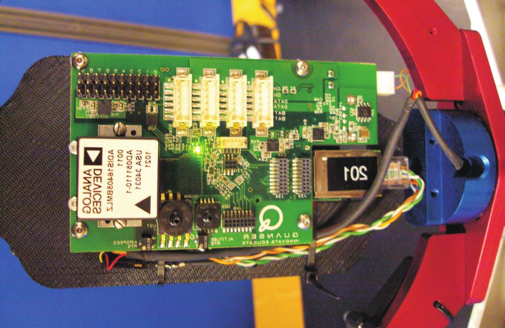
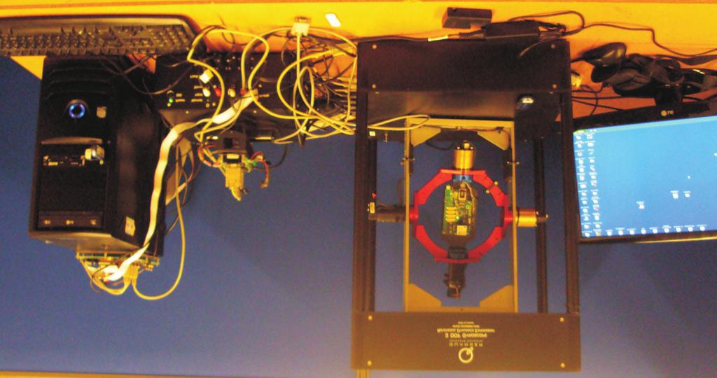
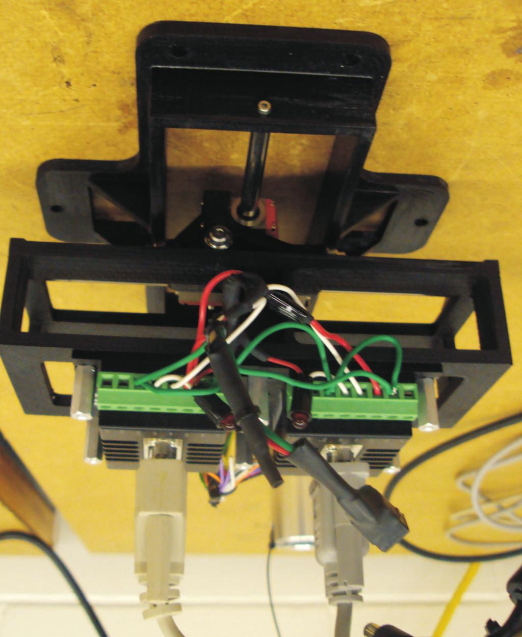
83 Chapter 6. Experimental Results Figure 6.2: Experimental setup. 75