Protein production. What can we do with ODEs

Transcription

1 Protein production What can we do with ODEs 2018

2 Modeling protein production with ODE We have seen various examples of wiring networks. Once you know how a regulatory network is wired in a particular way, systems of ODEs can be written and solved, providing a powerful tool for predicting how these regulatory networks will behave inside the cell. This lecture: two rather simple but very important examples (an unregulated gene and a negatively autoregulated gene). The same methods are used to analyse much more complicated networks with many tens of genes and proteins. Memo: Ignoring space, and compartmentalisation, we are making the important assumption that the interior of the cell (or a particular cellular compartment) is well mixed (this is ok on certain timescales, hence for certain processes, but will not always be the case!).

3 Consider: an A molecule collides with a B molecule, the two can react to produce a molecule of type C.

4 Consider: an A molecule collides with a B molecule, the two can react to produce a molecule of type C. In a small interval of time dt, the probability of a C molecule being produced is qn A N B /V, where V is the volume of the system, N A is the number of A molecules and N B is the number of B molecules. Note: the probability scales with 1/V since a pair of A and B molecules will be less likely to meet each other in a larger volume. Figures previous slide show simulations of this process. (q and V have been set = 1) If the numbers are small, the stochasticity in the process is important (randomness in the A+B collision and reaction times) and discrete events can be seen. Over next lectures, we will learn how to simulate this class of processes via an efficient algorithm.

5 If the numbers are large, then many events take place in a small time interval. We can assume the process continuous, and write: Note: this is a second order or bimolecular reaction (it involves two reacting molecules), the dimensions of the rate constant are (concentration 1 )(time 1 ). We also need to specify initial conditions, e.g. c A (0) = c B (0) = c 0 and c C (0) = 0.

6 Can write ordinary differential equation methods to understand how cells control the production of protein molecules from their genes. Here, we are interested in how the concentration, c P, of a specific protein molecule, P, changes with time inside the cell. Protein P is produced from its gene, gp, by transcription (to make messenger RNA) followed by translation (to make an aminoacid chain) and protein folding. We could model all of these processes in detail but for now let s just suppose that protein P is produced at a constant rate, k, as long as the gene, gp, is active. This reaction is zeroth order: the protein P is created at a constant rate that does not depend on any other variables in the model. The dimensions of the rate constant for this reaction are therefore (concentration)(time 1 ). We write this as a chemical reaction, source is actually the gene, gp, plus the whole machinery of transcription and translation. Here we just put this into a black box and assume that protein P is produced at a constant rate.

7 Protein molecules are also removed from the cell; This could be because another protein molecule actively degrades them or because the cell is growing and dividing into daughter cells (and every time the cell divides, a given protein molecule has a chance of being lost). For now, let s just assume that there is a fixed probability per unit time, µ, that any given molecule of P is removed. We can also write this as a chemical reaction: [a first-order or unimolecular reaction: a single molecule of P reacts. For unimolecular reactions, the dimensions of the rate constant are (time) 1. The sink here is another black box, could be removal into a daughter cell or degradation into unspecified products] we can write a differential equation for the rate of change of the concentration c P of P molecules: steady-state protein concentration, c (ss) P If you know k and m you can plot the rate of concentration change: (kere k=2 and m =1)

8 Steady-state concentrations are a very important property of regulatory networks, and quite often this is all that people focus on when they study a model for a particular regulatory network. The value of c (ss) P depends on both k and µ. If protein removal is due to cell division and if the average time between cell divisions (the cell cycle time) is τ, then For the bacterium E. coli on a good food source, τ is about 30 min, so µ is about 0.02/min. Protein production rates, k,vary greatly, from virtually zero to about 50/min. So the number of protein molecules in a cell (assuming that there is only one copy of the gene) can vary from zero to several thousand.

9 For the simple model discussed here, we also solve the model for the timedependent protein concentration, c P (t). This is important because genes can be turned on or off in response to signals, and we d like to know how fast the cell can respond to a given signal. The time-dependent solution for protein concentration in this model can be found by simple integration: Let s suppose that protein P is an enzyme that allows the cell to metabolise lactose. Initially, the gene, gp, is repressed because a repressor protein is bound to its promoter. We assume that initially no protein P is present: c P (0) = 0. At time zero, the cell detects some lactose and the repressor leaves the promoter, so the gene becomes activated. How quickly can the cell produce protein P and start metabolising lactose? If c P (0) = 0, then the dynamics is given by:

10 We define the rise time, t rise, as the time it takes for protein P to reach half of its steady-state value. Setting c P (t) to c (ss) P/2 and solving for t rise, we obtain: which becomes, when we substitute in c (ss) P= k/µ : i.e. the response time of this simple network is determined only by the proteinremoval rate. For bacteria, protein removal is usually due to cell growth and division. As we saw earlier, the removal rate, µ, is typically ln(2)/τ, where τ is the cell cycle time. So the response time for bacterial gene networks is typically of the order of the cell cycle time, which is at least 30 min.

11 ODE for negatively autoregulated gene Genes can be turned on and off by the binding of specific proteins to the DNA in the promoter region. In many cases, proteins actually turn off their own production (i.e. the protein product of a gene is a repressor that binds to its own gene and turns off protein production). This is an example of negative feedback and is called negative autoregulation. We saw in lecture 3 that for E.coli, and probably for other organisms too, negative autoregulation happens much more often than one would expect if the regulatory connections between genes were chosen at random. Why has negative autoregulation been selected by evolution as a favoured regulatory motif? To try to understand this, let s write down the equivalent differential equation model for a protein that represses its own production.

12 We anticipate a result from the next lectures: For a protein binding to a DNA binding site, the probability that the binding site is occupied is where c/c 0 is the concentration of protein (relative to some standard value, c 0 ) and Δe is the change in energy when the protein binds. We can define a dissociation constant, K d, as For low concentrations (where c/c 0 is very small), we can see that the probability p bound that the binding site is bound becomes proportional to the inverse of the dissociation constant: p bound c/ K d. This shows us that K d is actually just the equilibrium constant for the dissociation of the protein from its binding site. The reason why this proportionality does not hold at higher concentrations is that the binding site becomes saturated with protein.

13 The more strongly the protein binds to its DNA binding site, the more negative Δe will be. Strong negative autoregulation (large negative Δe) therefore corresponds to a small value of K d. Combining the equations above, we get and the probability that the binding site is unoccupied is given by: Returning to our differential equation for the production and degradation of protein, the production rate is now proportional to the probability that the promoter binding site is not occupied by protein:

14 We now have a nonlinear differential equation for the concentration of protein, c P (t). Let s find out what the steady-state protein concentration is. Plot of the rate of change of c P versus c P, for two values of the production rate k. Also plotted are the results for a gene without negative autoregulation. [The solid lines are for k = 2 and m = 1, and the dotted lines are for k = 4 and m = 1. The blue lines show the result without negative feedback (for the same k and m).] We see that as in the non-regulated case, when the protein concentration c P production dominates, while when the protein concentration is high protein degradation dominates over production. is low Again for one particular value of protein concentration production and degradation are balanced (d c P /dt = 0), and this is the steady-state protein concentration.

15 Negative autoregulation affects the steady-state protein concentration in two important ways. First, the steady-state protein concentration is lower for the negatively autoregulated gene (shown in red) than for the unregulated gene (shown in blue). Second, when we compare the results for two different values of the production rate, k (solid and dotted lines), we can see that for the unregulated gene the steady-state protein concentration depends strongly on k (in fact, we know from our calculations above that it is proportional to k); while for the negatively autoregulated gene, c (ss) P changes only a little when k is changed by a factor of two. Both of these effects have important implications for the performance of the gene, as we shall see.

16 More on negative autoregulation. To get an expression for the steady-state protein concentration c (ss) P for the negatively autoregulated gene, we set the rate of change of c P (t) to zero: Obtaining: 4 For very strong autoregulation (where K d is very small), the result reduces to: 4 shows c (ss) P as a function of the protein production rate, k, for several values of the dissociation constant, K d. As the negative autoregulation gets stronger (as K d decreases), the curves become flatter: the steady-state protein concentration becomes less dependent on the protein production rate.

17 More on negative autoregulation. In the cell, the protein production rate depends on the concentration of RNA polymerase, as well as the concentration of ribosomes, mrna degradation enzymes, etc. All of these factors vary from cell to cell and over time inside any given cell. We therefore expect the protein production rate to fluctuate within and between cells. For a gene without negative autoregulation, this will cause the protein concentration to fluctuate, since c (ss) P is proportional to the production rate k. This fluctuation problem can be avoided using negative autoregulation. Because the curve of c (ss) P versus k is much flatter in the case of negative autoregulation, the steady-state protein concentration will remain stable even if the intracellular environment (i.e. the protein production rate) fluctuates. In other words, negative autoregulation can make the performance of a gene robust to changes in protein production rate. You may have noticed that for negative autoregulation c (ss) P does depend on the dissociation constant, K d. Is this a problem for robustness? Probably not: we expect K d to fluctuate much less than k because K d depends only on how strongly the protein binds to its DNA binding site, which is determined by the structure of the protein and the sequence of the binding site.

18 More on negative autoregulation. Negative autoregulation also has an important effect on the rise time, t rise : the time the cell needs to turn the gene on (to the half-maximal protein level). We saw that for the unregulated gene this time was fixed by the protein-removal rate, t rise = ln(2)/µ. What happens for a negatively autoregulated gene? To calculate t rise, in principle, we should solve the full equation, but this is tricky analytically. If we look at early times, when c P is small, we can approximate c P (t)/k d < 1 then and if we also assume that autoregulation is strong we can substitute the previous result for c (ss) P, obtaining

19 More on negative autoregulation. As K d decreases (i.e. as the negative autoregulation becomes stronger), t rise decreases. This important result shows that negative autoregulation can help cells to respond more rapidly to changes in their environmental conditions than they would be able to without regulation. The units chosen in the plot here are rather arbitrary. To get a feeling for some real numbers, we have already seen that a typical protein-removal rate µ in a bacterial cell would be 0.02/min, so the rise time for a typical protein without negative autoregulation would be ln(2)/µ ( 35 min). While protein production rates and protein-dna dissociation constants can vary enormously, a realistic value for k might be 0.2 molecules/min per cell volume and K d might be 0.02 molecules per cell volume (for a protein that binds very strongly to its DNA binding site). The value of t rise for a negatively autoregulated gene, assuming these parameter values, would then be 12.7 min: almost a factor of three faster than the gene without negative autoregulation.

20 How are these measurements done, at population level? The chip size is of the order of 1 cm 2. The analysis consists of taking a cell sample, extracting all mrna in this (hopefully) homogeneous sample, and translating it to cdna (DNA that is complementary to the RNA, and thus identical to one of the strands on the original DNA). The cdna is labeled with a fluorescent marker. The solution of many cdnas is now flushed over the DNA chip, and the cdnas that are complementary to the attached single-stranded DNA-mers will bind to them. The DNA chip is washed and images (with pixel resolution) and the fluorescent light intensity thus measures the effective mrna concentration. Aside from noise and fluctuations, which we address later, how is the type of mrna present in a sample (a population) of cells measured? DNA microarray chips can be used. These are large arrays (tens of thousands) of pixels (dots). Each pixel represents part of a gene, by having of the order of single-stranded DNAmers, that are identical copies from the DNA of the gene.

21 Biochemical Noise Small number stochasticity

22 Small numbers Cells with identical genes and environmental factors can differ chemically. One way in which this can come about is because of reactions involving small numbers of molecules. This can be addressed very quantitatively.

23 Why is a chemical reaction noisy when the number of molecules is small? The reason is that chemical reactions are stochastic, or random. That is, the outcome is governed by probabilities, and there are sufficiently few molecules that there is no single overwhelmingly favoured outcome. In our box of A and B molecules (the cell), we do not know the exact positions and velocities of all of the molecules and so we do not know the exact time when a pair of A and B molecules will meet and react. The exact times when reactions happen and the exact sequence of reactions that happen can be different in repeat runs of the same experiment. Why is this relevant? Even in something as small as a bacterial cell, there are many billions of molecules, so why would these stochastic effects be important? In fact, stochastic effects can be very important in cells, because even though the total number of molecules in a cell is large, the number of molecules involved in a particular biochemical reaction network can be very small. For example, in slow-growing cells, there is only one copy of the DNA (so the number of molecules of a particular gene may actually be only one). The number of messenger RNA molecules in the cell corresponding to a particular gene can also be very small for weakly expressed genes, and some proteins are only present in small numbers. Biochemical reaction networks involving genes, mrna or proteins that are present in small numbers per cell are likely to be dramatically affected by small-molecule number fluctuations. We call these stochastic fluctuations biochemical noise.

24 Individual cells are not identical That biochemical noise really is significant for biological cells was illustrated in an important experiment by Michael Elowitz et al. in Engineered Escherichia coli (E. coli) bacteria carry two different coloured fluorescent reporter genes. These genes encode proteins that do not interfere with any cellular functions, but when excited by light of the right wavelength they fluoresce (i.e. they emit light of a longer wavelength). This can be detected in an epifluorescence microscope. Elowitz et al. measured the relative amounts of the two fluorescent proteins in individual bacterial cells. The question that they wanted to answer was: if two cells are genetically identical and experience the same environmental conditions, will they produce the same amount of the two fluorescent proteins?

25 Individual cells are not identical Image shows the results of one of their experiments. This is an overlay of micrographs of a group of E. coli cells growing on a semi-solid gel under the microscope. These cells all grew from a single ancestor at the start of the experiment so they are genetically identical. Presumably also all subject to very similar stimuli. The colours show the relative amounts of the two fluorescent proteins present in each cell: green represents protein 1 and red represents protein 2. Cells that are coloured yellow contain approximately equal amounts of proteins 1 and 2. It is clear from this image that these identical cells are different colours, showing that they are very far from identical in their levels of production of the fluorescent proteins. Elowitz et al. also showed that cells that produce the reporter proteins at low levels (small number of molecules) have much more noisy levels of expression than cells that produce the proteins at high levels (a large number of molecules). This is what we would expect if differences between cells are caused by small molecule number noise, since s = 1/ N is larger for small N.

26 Intrinsic and Extrinsic Noise Are the differences between cells really caused by small molecule number noise in the chemical reactions involved in protein production (transcription and translation)? Or are the different colours caused by differences between the cells? For example, we can see in the microscopy image that some cells are short because they have just been generated, while others are much longer and are about to divide. Perhaps this affects the level of protein expression? Cells could also contain different concentrations of RNA polymerase or ribosomes, which would cause them to produce more or less fluorescent protein.

27 Intrinsic and Extrinsic Noise Precisely to explore the origins of the different amounts of the proteins, Elowitz et al. used two fluorescent proteins (in different colours) instead of just one. Within each cell, the genes encoding the two proteins should experience the same cell volume, RNA polymerase, ribosome concentration, etc. So if the differences in protein expression are caused by differences between cells, the levels of the two colours should be correlated: cells with a lot of protein 1 should also have a lot of protein 2. However, if chemical reaction stochasticity is responsible for the differences in protein expression, we would not expect the levels of protein 1 and protein 2 in individual cells to be correlated.

28 Intrinsic and Extrinsic Noise In fact, by measuring the amount of correlation between the levels of proteins 1 and 2 in individual cells in their experiments, Elowitz et al. could measure how much of the cell-to-cell variation is caused by differences between cells (which they called extrinsic noise) and how much is caused by chemical reaction stochasticity (which they called intrinsic noise). In their experiments, both sources of noise played a significant role. Why does it matter that genetically identical cells can have different levels of protein expression? One reason is that biochemical noise limits how precisely cells can control their own behaviour. If a cell needs to control precisely the concentration of a particular protein, either it must produce a large number of molecules (which is expensive) or it must use a biochemical control circuit (such as a negative feedback loop) to reduce the noise. On a more positive note, biochemical noise may actually be useful for cells in some cases. For example, bacterial populations are often exposed to environmental stress (attack by antibiotics, changes in food availability, etc). If all of the cells in the population are identical in their protein composition, the stress may wipe them all out; but if there is large variability in protein composition among cells, it is possible that a few cells will happen to have the right protein levels to survive the stress. The population can then regrow from these cells once the stress is over.

29 Elements of modeling noise

30 Noise - Birth-death model for gene expression For stochastic chemical reactions, we cannot predict exactly which reaction will happen when, or which cell in a population will contain which exact numbers of molecules of proteins, mrna, etc. However, we can make predictions about probability distributions. For example, we might predict the probability that a randomly selected cell in a population will have 100 molecules of a particular protein, even though we cannot predict which cell this will be. The quantity we are interested in is therefore p(n, t): the probability that our system contains N molecules of protein P at time t. We can write down an equation for p(n, t) for the simple one-step model of gene expression that we discussed above, in which we include chemical reactions for protein production and degradation: We assume that these reactions are Poisson processes. This means that if we observe the system for a very short time interval from time t to time t + dt, the probabilities that the first reaction (production), or the second (degradation) happen will be:

31 Noise - Birth-death model for gene expression Considering all the (4) ways in which the number of proteins can change, we have: You can check that the steady state solution is: a Poisson distribution! As (k/µ) increases, the average number of molecules increases. The mean and standard deviation σ N of the distribution p(n) are given by: Can estimate the importance of stochastic effects considering the ratio of the standard deviation to the mean:

32 Noise - A two-step model for protein production The model that we have just been considering may be too simple. In reality, the production of protein from a gene does not happen in a single step. We can make our model slightly more realistic by making a two-step model that includes both transcription and translation. The reaction scheme for this model would be Here, M represents mrna and P represents protein. It is possible to write down a chemical master equation also for this model, and to solve it for the steady state probability distribution. In this case, there is a probability distribution for the number of messenger RNA molecules as well as for the number of protein molecules. For mrna we only need to consider the top two reactions (since the bottom two reactions do not change the number of mrna molecules), which are identical to our previous simpler model. So we expect the probability distribution for the number of mrna molecules to be a Poisson distribution. However the bottom two reactions, which control the production and degradation of protein, are now different from our simple model. This means that the probability distribution of protein may be different from a Poisson distribution in this model.

33 Noise - A two-step model for protein production Let s set the parameters (translation rate/mrna decay rate) so that five proteins are made on average per mrna molecule (although some mrna molecules will produce more and some less). We can compare this with the previous one-step model by fixing the transcription rate so that the average protein number is the same in both models. The results are shown in the plot: We can see immediately that the distribution is broader in the two-step model, i.e. this model predicts more noisy protein expression than the one-step model. The reason for this is that the extra chemical reaction step amplifies the noise: the number of mrna molecules is itself noisy, and then on top of this each mrna molecule can produce a variable number of proteins.

34 Visualising Noise in expression How can we test whether these are good models for noisy gene expression in real cells? One way to do this is actually to carry out single molecule experiments, in other words to watch, under the microscope, the production of single protein molecules in individual cells. Since protein molecules are very small, this is a very challenging task. However, in 2006, Yu et al. managed to design an appropriate experiment. They made a strain of E. coli that produced a yellow fluorescent protein attached to a polypeptide (a chain of amino acid molecules), which could anchor this complex in the cell s lipid membrane. When the fluorescent protein is anchored in the membrane, it diffuses around much less, making it easier to see single molecules under the microscope. In this system, using advanced fluorescent microscopy, it is possible to see individual fluorescent protein molecules as dots within the cell membrane. Yu et al. could then grow cells under the microscope and track the moments when individual dots appeared in the membrane. In this way, they could see the production of individual protein molecules in real time. To keep the protein numbers low, the researchers included a binding site for the Lac repressor protein. When this repressor protein is bound to the operator site in front of the gene that encodes the fluorescent protein, no protein will be produced.

35 Visualising Noise in expression The bacterial cells in the series of images grow from a single cell during the experiment. The yellow dots show individual protein molecules bound to the cell membrane. By tracking the appearance of these dots, Yu et al. were able to monitor the moments when protein molecules appeared in the membrane.

36 Visualising Noise in expression This was done for different cell lineages, as shown in the plot, which indicates the number of protein molecules that were produced in a 3 min interval. The dotted vertical lines show the moments when the cell divided into two daughter cells. What s really striking about Yu et al. s results is that for most of the time, no protein molecules are being produced. Protein production occurs in short bursts, with long intervals where nothing happens. This is probably because most of the time the Lac repressor protein is bound to the DNA, thereby preventing protein expression. The bursts of expression take place during the rare moments when a stochastic fluctuation causes the repressor to fall off its DNA binding site. Yu et al. s setup therefore allows us to see stochastic chemical reactions happening inside biological cells, in real time and at single-molecule resolution.

37 We have focused here on noise in gene expression, but the stochasticity of chemical reactions is also important in many other cell functions. Single-molecule experiments have revealed the effects of biochemical noise in the molecular machines that drive the flagellar motor that allows cells to swim and in the bacterial membrane receptors that sense environmental gradients. Other experiments have found important effects of biochemical noise in the development of fruit-fly embryos and the mechanisms that control whether or not cells proliferate. It seems that noise is everywhere.

38 Essence of regulation The control of a cell s chemistry

39 In simple cases, we can match the regulation circuit to the actual molecular processes, and hence have a handle on e.g. the rates through a model that has the real physics.

40 The l-phage switch: the study of developmental decisions started here In simple cases, we can match the regulation circuit to the actual molecular processes, and hence have a handle on e.g. the rates.

41 If proteins have ~ 300 amino acid chains, then 900bp per protein, and around 4500 genes. This is ~ true, in E.Coli. This is the lac operon: the study of gene regulation started here.

42 This is the lac operon: the study of gene regulation started here.

43 How do we measure gene expression? O-nitrophenyl b-galactoside (A) Bulk (population): measurement of enzyme activity Colorless can be cleaved by b-galactosidase to become yellow (B) Single cell: Make a construct where the promoter drives expression of a fluorescent protein, like GFP. Microscopy.

44 How do we measure mrna levels? Microarray or PCR bulk techniques. Can also get mrna levels at single cell, see p of Nelson

45 Timescales for various reactions in the transcription network of a bacterium 1ms binding of small molecules (signals) to transcription factors, thus changing the transcription factor activity 1s 5min binding of transcription factor to its DNA site transcription + translation of the gene ~1hr (i.e. 1 cell generation) 50% change in the concentration of the translated protein (assuming no degradation, i.e. for stable proteins) U.Alon, p11

46 Repressors hinder the binding of RNA polymerase, or the initiation of transcription. Renditions, to scale with DNA, 4 different repressors. Obtained from X-ray crystallography. Many such structures LMB

47 Activators promote the binding of RNA polymerase.

48 Stat Mech can be used to describe quantitatively the activity of promoters.

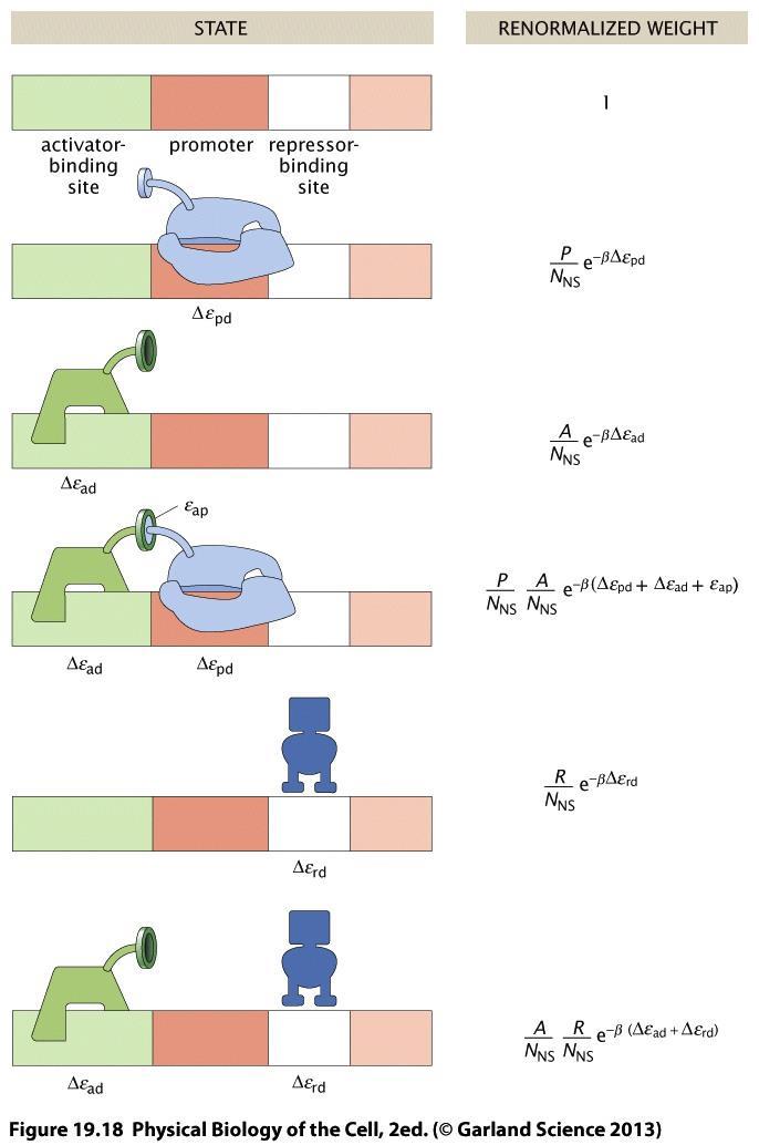
49 Stat Mech - case of no regulation. [Full details see Phillips or pdf notes.] RNA polymerase binding to a specific site: RNA polymerase binding: competition between specific and non specific site: This extends the case above seen in lecture 5. Assume the non-specific sites on the DNA are N NS boxes. Then the partition function associated with these states is: where e NS pd is the energy of binding the polymerase to a non-specific site (and e S pd will be later the energy of binding the polymerase to the specific site ). Now we can write the total partition function. We need to sum over the states in which the promoter is occupied (hence P-1 polymerase molecules in the non-specific sites), and those where it is not: The ratio of configuration weights where promoter is bound, to all weights, is:

50 Stat Mech - case of no regulation (cont). The factorials can be simplified for N NS >>P, and we can write the result to show that only the energy difference matters: Familiar result for two-state models, with the unoccupied state of the promoter having weight =1, and the occupied having weight P/N NS exp( βδe pd ). The energy differences Δe pd are negative, and can range between minus a few to 10 k B T. Stat Mech - case of activation. Activators are proteins that bind to a specific site, and promote the recruitment of RNA polymerase to a nearby promoter site. We now have 4 classes of outcome to sum over to make the total partition function: the activator and promoter site can each be occupied or unoccupied. So: Notation: A, a are the activator, P, p the polymerase, d the DNA). e pa is the energy that favours the activator and the RNA polymerase being close.

51 Stat Mech - case of activation (cont). Algebra more lengthy but follows the exact steps as previously. To get promoter occupancy, we can take the ratios of the weights of the two favorable states, against the sum of all weights, and we get: With Δe the energy differences between specifically and nonspecifically bound conditions and e Neat result! Shows that activating molecules make an F > 1, i.e. have an effect that is mathematically equivalent to increasing the number of polymerases. Given realistic values of the other energies, a few k B T for e ap is enough to significantly change the bound probability. If the approx (N NS /P F reg )exp(βδ e pd ) >> 1 holds, i.e. the promoter is not too strong, then you can obtain (exercise) that the fold increase is approximately F reg (A) itself. Details of the promoter (its binding energy) factor out of the problem!

52 Activation. The stat mech model shows that the presence of activators is equivalent to having a higher concentration of polymerase.

53 Activation. The probability of binding, which is a good proxy for the rate of expression, depends strongly (`fold increase ) on the polymeraseactivator binding. In plots like this, all other parameters are fixed. Here: P=500, De pd = -5.3k B T, De ad = k B T.

54 Clever experiments have been carried out to specifically target aspects of the activator-polymerase interaction, which correspond directly to how we write the stat mech models.

55 Stat Mech - case of repressor. Repressor proteins occupy the promoter region, and prevent the RNAP binding there. Physics model is another variant of previous partition function machinery We get And further simplifed as done for the activator, but this time with Δ e rd = e S rd e NS rd. Here, F reg < 1, which means that the systems behaves as if fewer polymerases were present.

56 Repression.

57 Measurement of fold-change in repression.

58 Segmentation and single cell quantification of fluorescence

59 Taking care (same settings, removing autofluorescence background, etc) it is then possible to quantitatively compare across different conditions: a measurement of fold-change.

60 Stat Mech - case of activator and repressor together. In a real regulatory mechanism there will be both activation and repression, in competition. This tests our algebra skills there are 6 cases to sum over: We can follow same steps, with patience, and get: With now a very rich regulation function:

61

62 Model and experiment with both positive and negative regulation De ad = -10k B T, De ap = -3.9k B T, De rd = -16.9k B T. This is lac operon experiment, from 2007 PNAS paper. Rather than change number of activator and repressor molecules in a cell, it is easier to modulate their binding to DNA. IPTG blocks the repressor from binding, camp promotes the activator CAP binding.

63 What is lac operon? The lac Operon is a system that allows bacteria to react to the best sugar present, specifically to ensure that the enzymes to digest lactose are produced only when glucose is not present, and lactose is present. It seems an apparent simple objective, but selecting reliably for one of four situations requires a mechanism of both activation and repression as outlined here. This regulatory system has played a key role historically in understanding physical and biological aspects of gene regulation, and is still subject of quantitative investigations and modelling today. In the lac Operon there is an activator, the protein CAP. In order to recruit RNAP, CAP has to be bound to a molecule called cyclic AMP (camp), whose concentration goes up when amount of glucose decreases. There is also a repressor, the Lac repressor, which decreases the amount of transcription unless it is abound to allolactose, a byproduct of lactose metabolism. IPTG is a synthetic inducer, also binding to the repressor.

64 Zooming in on lac operon Manipulating the lac operon to dissect repression effects due to affinity Fitting with the simple repression model, we obtain -16.9, -14.4, kt for O1, O2, O3

65 In the lac operon DNA looping also important

66

67 All parameters are known except the looping free energy which is obtained by these fits.

68 A summary of regulatory architectures presented so far

69 Rich diversity of factors that can regulate gene expression

70 Memo: Absolute numbers of various critical molecules are not large

71 Transcription is not a steady state: it occurs in `bursts

72 Noise - Birth-death model for gene expression Considering all the (4) ways in which the number of proteins can change, we have: You can check that the steady state solution is: a Poisson distribution! As (k/µ) increases, the average number of molecules increases. The mean and standard deviation σ N of the distribution p(n) are given by: Can estimate the importance of stochastic effects considering the ratio of the standard deviation to the mean: Slide from earlier lecture master equation for an unregulated promotor

73 We have made models based on molecular numbers. Markov chains. Now we have a molecular/physics picture of the underlying process.

74 Data of mrna in E. coli

75 Stochastic modeling - The master equation approach is only analytically tractable in very selected cases - A numerical brute force approach with fixed discrete time intervals is wasteful because need Dt smaller than inverse of any rates, and any fluctuations that one want to track. This means *many* Dt typically wasted with the system not changing state, particularly when small number of reactants. - Better approach: have a strategy for adapting Dt - Gillespie approach: randomly assign the time to the next reaction, from a probability distribution. This avoids timesteps where nothing happens. - This creates a realisation of the stochastic time evolution of the system. Running several iterations gives distributions. - Particular example A B (Daniel Gillespie, Physicist, published milestone paper 1976)

76 Simulating efficiently networks of reactions: the Gillespie algorithm. Particular example: 2 random numbers: Step 1- choose Dt to next reaction; Step 2 biased choice of which reaction

77 Gillespie algorithm We want a timestep Δt, and we want to determine P (i, Δt)dt, the probability that reaction i takes place in the interval [Δt, Δt + dt ]. First, we note that we also want to impose no reaction to have occurred before Δt. We call this probability P 0 (Δt). Thus the probability that reaction i takes place in the interval [Δt, Δt + dt] is: Need to calculate P 0 (Δt): Taylor expand first term, so get: And hence: [ P 0 (Δt = 0) = 1 and k 0 = S i k i ]

78 Gillespie algorithm (cont) Substituting back, we get If we sum this over all i, we get the probability that any of the possible reactions happens in the interval Δt, Δt + dt: This is the distribution from which one needs to pick Δt. Now need to work out how to make a distribution from which to pick the random choice of which reaction takes place. The probability that reaction i happens at some time is: This gives us the criterion to choose (randomly, but with the right bias) which reaction will take place at the simulation timestep.

79 The unregulated promoter (see also back to first lectures of this set). There are two reactions (i=1,2): (1) an mrna can be can be produced, with probability k per unit time; (2) an mrna can decay, with probability γ per unit time and per unit molecule. Call m(t) the number of mrna molecules at time t. Rates are k 1 = k and k 2 =m(t) γ.

80 Efficient way to simulate networks. {q i }={D, r, p} These examples from Intrinsic noise in gene regulatory networks Thattai and van Oudenaarden, PNAS 98, (2001)

81 Dynamical Systems Circuits, switches, oscillations

82 General framework and useful tools We examine, in turn, the one-variable system ( flow on the line ), the two-variable system ( flow on the plane ) and the three-variable system ( 3-D flow ). In general, an n-variable system requires n equations to represent it. The dynamics of a general non-linear system can be described by a set of coupled differential equations: For example, damped harmonic motion with the second order (linear) DE: can be written a set of coupled first-order equations as:

83 Flow on the line We begin by examining one- dimensional flow, that is, the dynamics of a single first-order DE, Fixed points of a 1-D flow The function f is single-valued for all x. The dynamics therefore take place along a line (the x axis). In the notation of Strogatz, the phase-plane plot represents a vector field on the line: the velocity vector dot-x is shown for every x. The trajectory is a plot of dot-x as a function of x. The time coordinate is thus implicit we could, for example, mark off time ticks along the curve given any starting value of x, and hence dot-x, but the main properties of the system are apparent directly from the phaseplane plot.

84 Flow on the line - cont Fixed points of a 1-D flow We can immediately identify two types of fixed point. These are values of x for which x is zero, so that the system is, momentarily at least, at rest. A stable fixed point results whenever dot-x is zero and the slope of the dot-x vs x curve d (dotx)/dx is negative. This ensures that for small fluctuations away from the fixed point, as shown in green arrows on the plot, the velocity dot-x is in a sense to bring the system back to the fixed point. A stable fixed point is also known as a sink or an attractor. An unstable fixed point, on the other hand, has d (dot-x)/dx > 0, so that small fluctuations result in a motion directed away from the fixed point. Other names for an unstable fixed point include source or repeller. One other type of fixed point is possible, and is known as a half-stable point.

85 Example of Autocatalytic chemical reaction This is a non-linear dynamical system. The presence of X stimulates further production of X hence the term autocatalytic. This is one model for the growth of amyloid plaques in the brain in diseases such as BSE and CJD: the presence of a small amount of plaque, X, catalyses the conversion of normal protein, A, to plaque. There are two variables in the process: a, the concentration of reactant A, and x, the concentration of reactant X. If the concentration of A is always large, then it will be effectively constant. The problem then reduces to dynamics in one variable. Given the rate constants for forward and reverse reactions, k 1 and k 2, the equation governing the dynamics is

86 Example of Autocatalytic chemical reaction-cont The trajectory in the phase-plane can be plotted: It is also straightforward to sketch the concentration vs time: Here, x and a are dynamical variables: that is, they are the variables which change with time. The two other variables, k 1 and k 2, are control variables. In this particular case, varying the control variables does not change the general character of the dynamics, but only the details. Since dot-x is linearly proportional to x in the vicinity of the fixed points, the approach to equilibrium must be exponential.

87 Control variables Consider now the system described by As a is increased from a negative value, the two equilibria (one stable, and one unstable) first approach each other, then merge to form a half-stable fixed point, and finally annihilate. The control parameter, or variable, a, thus determines the stability of the system. We are interested in situations, such as that shown above, where a change in one or more of the control parameters leads to discontinuities, i.e. qualitatively different dynamics, such as a change from stable to unstable behaviour. This is the basis of Catastrophe Theory. The key result from catastrophe theory is that the number of configurations of discontinuities depends on the number of control variables, and not on the number of dynamical variables. In particular, if there are four or fewer control variables, there are only seven distinct types of catastrophe, and in none of these is more than two dynamical variables involved. Now we consider all cases up to two control parameters. For simplicity we restrict ourselves to a single dynamical variable, x, with little loss of generality.

88 Dynamics from an effective potential We can look at the dynamics in terms of an underlying potential, which we shall here denote by V (x). Stable equilibria are local minima in V (x), unstable equilibria are local maxima and half-stable fixed points are points of inflection. We are dealing with the evolution of arbitrary dynamical systems (as loosely interpreted), and hence there may not actually be a true potential energy (in mechanical systems there often is one). In terms of the equation, we can define the potential to be: For a first-order system (and hence one-dimensional motion) we have to imagine a particle with an inertia which is negligible in comparison with the damping force. The negative sign implies that the force on a particle is always downhill, towards lower potential. This can be shown simply by applying the chain rule to the timederivative of the potential and applying the definition of the potential:

89 Dynamics from an effective potential - cont Thus V (t) decreases along trajectories (in example of a particle, it always moves towards lower potential). In summary, the potential has the following properties: (1) dv/dx is force-like (i.e., is in the direction of motion). (2) Equilibrium positions, x* (fixed points) are given by dv/dx = 0. (3) The stability of the fixed point is determined by the sign of d 2 V/dx 2 x*. Forms of the potential curve The potential function can always be approximated by a Taylor series, so that V (x) = a + bx + cx We can ignore a, since it is just a constant and does not affect the dynamics. In the vicinity of a single fixed point (i.e. equilibrium) we can also eliminate b by shifting the coordinate system to put the fixed point at the origin (although b cannot be ignored for multiple fixed points). This leaves us with V (x) = cx 2 + dx 3 + ex We can now enumerate the possibilities.

90 Potentials give rise to specific instabilities (1) Harmonic Potential. This is the simplest possible form, and the only one possible for purely linear systems: V (x) = αx 2. There is a single fixed point, x = 0, for all α. If α > 0 then the fixed point is stable; if α < 0 then it is unstable. (2) Asymmetric cubic potential: The saddle-node bifurcation. The potential has the form V (x) = αx + x 3. For α > 0, no equilibrium position is possible. For α < 0, then there is always one stable and one unstable equilibrium. Here we introduce the idea of control space. We can plot the location of the fixed point, x, as a function of the control parameter, α: On the control space plot, the solid line denotes the location of the stable equilibrium, while the dashed line indicates the locus of the unstable equilibrium, both as a function of α. The form of the instability shown here is what Strogatz calls a saddle-node bifurcation, and sometimes known as a limit point instability or a fold. The phase-plane trajectories for this system were shown earlier, for the system with dot-x = x 2 + a. This is the origin of the term saddle-node bifurcation as a is decreased through zero the fixed point is first created, and then bifurcates into two: one stable and one unstable.

91 Potentials give rise to specific instabilities - cont (3) Cubic potential with quadratic term: The transcritical bifurcation. The potential this time includes a term in x 2 rather than a linear term as in the previous section. V (x) = x 3 + αx 2 The effect of this is to give a double root, and hence a fixed point, at the origin, regardless of the location of the third root. This is generally known as the transcritical bifurcation. One physical example of such a system is the laser. (4) Symmetric quartic potential: The pitchfork bifurcation. The potential is: V (x) = x 4 + αx 2. Two cases: For α 0 there is just one stable equilibrium; For α < 0 there is one unstable equilibrium and two stable equilibrium points. Plotted on the side here is the case of positive term on the 4 th power. In this case we refer to the Stable Symmetric Transition. It is also known as a Pitchfork Bifurcation (see Strogatz) from the shape of the bifurcation diagram, as shown at right. One example of this sort of potential is the Euler strut. If we take the negative sign on the 4th power, the additional quartic term may also act to destabilize the system, and the locus of the fixed points changes qualitatively (exercise).

92 Potentials give rise to specific instabilities - cont (5) Asymmetric quartic potential with two control parameters: the Cusp catastrophe. We now consider an asymmetric potential, of the form V (x) = αx 2 + x 4 + βx where the βx term introduces asymmetry to the symmetric quartic form of the previous case. We now have two control parameters, α and β. Depending on the sign of α, then, we get two different sorts of behaviour. If α > 0 then the linear term merely shifts the position of the fixed point, but does not qualitatively change the dynamics from that of a simple harmonic potential. If α < 0 however, the linear term can eliminate the unstable fixed points and one of the stable fixed points as well.

93 Potentials give rise to specific instabilities - cont (5) -cont. Asymmetric quartic potential with two control parameters: the Cusp catastrophe. The control space diagram is now two dimensional. Consider the equilibrium surface, or a plot of the location of x against α and β. The bifurcation set is the set of points in the (α, β) plane dividing the plane into different regions of stability, and has a characteristic cusp shape. As we move from the shaded to the nonshaded region (i.e. across the bifurcation set), there is a sudden change in behaviour, with marked hysteresis when the path is reversed.

94

95 Two dimensional systems e.g. harmonic oscillator

96 We have seen fixed points. Their stability can be determined by linearising the system and looking at eigenvalues (real parts) of the matrix of partial derivatives. Two other important concepts in nonlinear systems are phasespace and nullclines. Phase space For 2 coordinates, the phaseplane is a sketch of the system time evolution in (x; y) coordinates. This is different from a sketch against time which is the way you often see data. Phaseplanes can provide much more useful info, such as a global way of looking at your system. Nullclines The latter are curves that enable one to break the plane into regions of different qualitative behaviour. If 2 variables x =f(x,y), y =g(x,y), then nullclines are f(x,y)=0 and g(x,y)=0, and their crossing points are the fixed points.

97 Notice that x and y have defined sign in the regions identified by the nullclines, so a lot of the system behaviour can be determined at a glance. e.g. could fill in these phase planes with qualitative trajectories, and determine the stability or instability of the fixed points.

98 Two dimensional systems general linear case In matrix form: 2 ways to deal with this: a) Find new variables that decouple the two equations (diagonalise). These will still be linear response, so solutions will be exponential decay (or rise). b) Turn into a second order equation and examine stability Generally where T is the trace of A and is its determinant. This can then be treated with e.g. Laplace transform, giving us the poles in the complex plane.

99 Two dimensional systems general linear case there are only 5 possibilities:

100 The non-linear two-variable case exhibits one other possibility: a periodic orbit known as limit cycle. The limit cycle is defined as an isolated, closed trajectory. That is, neighbouring trajectories are not closed. It is an attractor if neighbouring trajectories spiral towards it, or a repeller if they spiral away. Note that not every non-linear oscillation is a limit-cycle. Many examples like the harmonic oscillator or prey-predator oscillations do not attract nearby points in phase-space.

101 Example of trajectories in a general twovariable system. x=f(x). There are a number of fixed points, i.e those for which x=f(x) = 0. A and B are saddle nodes; C is an unstable node (giving rise to the unstable spirals); D is a limit cycle that is, an isolated closed trajectory. Spirals internal and external to D are both attracted towards it.

102 Switches in genetic circuits Gardner et al, Nature 2000 IPTG, a lactose analog, is an inducer that flips the switch (we saw IPTG binds to the Lac repressor and reduces its affinity). Note: bistability, not a continuous change. The bimodality occurs due to natural fluctuations in gene expression and the close proximity of the toggle switch to its bifurcation point.

103 Switches in genetic circuits: 2 repressor proteins mutually regulated

104 Mathematical model for this genetic switch c 1, c 2 the two repressor protein concentrations. Both proteins can degrade, rate g To model the repression on 2, consider a modified expression rate of form r(1-p bound ), where r is a basal rate. If binding is a Hill function, Then the reaction system is: This system has 2 ranges of parameters giving different behaviours. A) a range giving a single stable solution, with equal concentrations of both proteins. B) a range giving two well distinct protein concentrations. If the parameters are in the range of (B), then the network exhibits switch like behaviour. The system can be made dimensionless (with a = r K b 1/n / g and time in units of 1/ g ):

105 Mathematical model for this genetic switch (cont) One solution is always Can work out if there are other solutions. Take n=2 to proceed simply. For u*, and similarly v*: Thus: The cubic polynomial here can be shown to have only one zero, and by some inspection you can see that it is the solution with u* = v*. The quadratic however can have 0 (if α < 2), 1 (if α = 2), or 2 (if α > 2) solutions, depending on the value of α. In the 2-solution regime, the concentrations are not the same! The solution with u* = v* exists for all α, but it is unstable for α > 2. Can calculate phase portraits of this system: y=u 3 +u-a y=u 2 -au+1

106 Calculate these in Matlab a=1 a=1 a=3 a=3 So, a=2 separates region with one single solution of equal concentrations, against having two stable distinct solutions and one unstable.

107 Oscillations in genetic circuits One simple set of equations that gives rise to oscillations is a gene regulated by both an activator and a repressor: - the repressor binds as a dimer, and represses production of the activator - the activator also binds as a dimer, and increases the production of itself, and also of the repressor. Then the rate equations can be written as: Where r 0A, r 0R are the basal expression rates, and r A, r R are the regulated rates in the presence of the activator bound. Can be made nicely dimensionless:

108 Oscillations in genetic circuits (cont) Activator gene, with positive feedback on itself Repressor gene, stimulated by the activator

109 Oscillations in genetic circuits (cont) Dimensionless system: Oscillations can arise if there is a separation of timescales between the activator and repressor dynamics. Nullclines are the locus of points achieved by the repressor or activator at steady state, given fixed values of activator or repressor, respectively. They are obtained by setting the time derivatives equal to zero, and we have:

110 Oscillations in genetic circuits (cont) Limit cycle Initial transient Note different timescales: Nullclines Repressor is much slower to equilibrate This is an example of a relaxation oscillator

111 Natural Oscillators 1. Circadian rhythms (eg Drosophila, 24 hour period, feedback oscillator) 2. Ca++ Oscillations 3. Glycolytic Oscillations * (relaxation oscillator) 4. Signalling Pathway Oscillations (P53, ERK, NF-kB) 5. Cell Cycle (relaxation oscillator) 6. Synchronous Rhythmic Flashing Of Fireflies 7. Segmentation during development 8. Many examples of chemical oscillators (mostly relaxation oscillators) 9. Motile Cilia in the airways and in the brain 10.. Buck, John; "Synchronous Rhythmic Flashing of Fireflies. II," Quarterly Review of Biology, 63:265, 1988 * During growth phase on glucose and ethanol, starve yeast of glucose, add cyanide and glucose, the glycolytic pathway will oscillate (NAD/NADH, ATP/ADP)

112 Many signals oscillate in cells experimental importance of single cell imaging.

113 Case of NF-kB Transcription factor translocates repeatedly between cytoplasm and nucleus of innate immune cells. This is just downstream of the sensor for infection, and serves as the trigger for fast innate immune response: inflammation. The nuclear factor kb (NF-kB) transcription factor regulates over 300 genes.

114 Experiment: cells were subject to pulsatile inflammatory signals. Observed synchronous cycles of NF-kB nuclear translocation. Lower frequency stimulations gave full-amplitude translocations, whereas higher frequency pulses gave reduced translocation, indicating a failure to reset. Deterministic and stochastic mathematical models predicted how negative feedback loops regulate both the resetting of the system and cellular heterogeneity. Altering the stimulation intervals gave different patterns of NF-kB dependent gene expression, supporting the idea that oscillation frequency has a functional role.

115 Tying some threads together, and getting closer to research themes Taming protein production bursts Noise in dynamical systems Beyond model experiments in bacteria

116 Noise at the protein level can be evaluated analytically. In particular, it can be quantified measuring the relative fluctuations with the coefficient of variation CV p = σ p / p (where p represents the protein level), which for a constitutive gene takes the simple form CV p sqrt[ (1+b) / p ], where the mean protein level is simply given by the product of the average size of bursts and their frequency: p = b a.

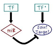
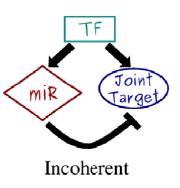
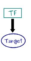
117 microrna (mirna) We have assumed so far regulation of protein production by Transcription Factors (TF) proteins regulating promoter region activity. This is the main regulatory mechanism, but does not account for everything. Post-transcriptional regulation (and post-translational) mechanisms also exist. Why? An important mechanism is played by microrna. MicroRNAs are non-coding RNAs that negatively regulate the protein production of their mrna targets in metazoans and plants. They are rather small (about 22 nucleotides long), single stranded RNAs, and are known to target a substantial portion of the human genome. In bacteria, there are similar short single strands of RNA with regulatory function, called srna.

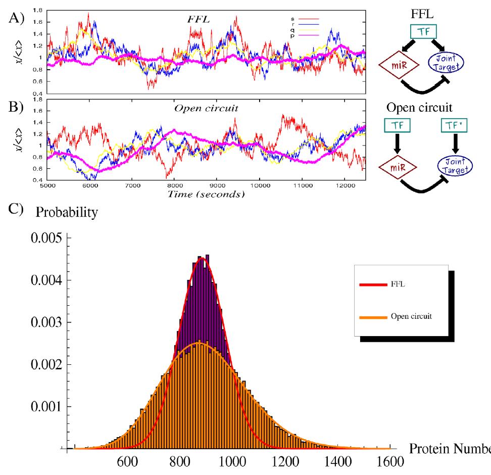
118 We have seen self-regulation as a vastly overrepresented motif. Another is the microrna-mediated feedforward loop in which a master transcription factor regulates a microrna and, together with it, a set of target genes. It can be shown analytically and through simulations that the incoherent version of this motif can couple the fine-tuning of a target protein level with an efficient noise control, thus conferring precision and stability to the overall gene expression program, especially in the presence of fluctuations in upstream regulators. A nontrivial result is that the optimal attenuation of fluctuations coincides with a modest repression of the target expression. This feature is coherent with the expected fine-tuning function and in agreement with experimental observations of the actual impact of a wide class of micrornas on the protein output of their targets.

119

120 Tying some threads together, and getting closer to research themes Taming protein production bursts Noise in dynamical systems 1 st example Beyond model experiments in bacteria

121 Noise control with microrna so what can they do [Osella et al., Front. Genet., 06 October 2014] Gene expression is inherently a stochastic process, so fluctuations in protein concentration can induce random transitions between the alternative steady states of a bistable genetic circuit like the toggle switch. A bistable circuit at the basis of cell fate determination is expected to be robust to these stochastic transitions, since they could in principle drive the cell to an undesired phenotype. mirna regulation can control the stochastic transitions between the two alternative steady states of a toggle switch. A major source of stochasticity in gene expression is due to the burstiness in protein production because (a) during the lifetime of a single mrna several proteins can be produced, and (b) there are bursts of transcription, probably due to transitions in the promoter state. A fluctuation at the transcriptional level can be amplified by the translation of a large protein burst stemming from a single mrna. The average size of these bursts b is given by the product of the rate of translation k p and the average lifetime of mrna 1/γ m (i.e., b = k p /γ m ), while their frequency a is defined by the transcription rate k m with respect to the timescale set by protein degradation γ p (i.e., a = k m /γ p ).

122 Regulation at the transcriptional level, e.g. by transcription factors, modulates the transcription rate of the target genes, thus affecting the burst frequency a. On the other hand, mirnas exert their action by suppressing translation (i.e., decreasing k p ) or promoting mrna degradation (increasing γ m ). Both regulative modalities affect the target burst size rather than the frequency. Therefore, the same degree of repression exerted transcriptionally or posttranscriptionally via mirnas will lead to very different levels of noise of the target protein concentration. In particular, the expression for the coefficient of variation suggests that mirnas, by reducing the target burst size, are more effective in keeping fluctuations in gene expression under control. These simple arguments indicate a possible evolutionary reason to prefer mirna regulation, instead of transcriptional regulation, to build toggle switches involved in cell fate decision: robustness to stochastic fluctuations is probably a crucial feature.

123 mirna regulation is an example of molecular titration since it requires the direct oneto-one binding of a regulator and its target molecule (different from transcriptional regulation, where even a small amount of transcription factors can influence the target production with no significant consequences on their concentration). The equations (not empirical - physically justified!) can be written for this situation, terms are slightly different from TF. ( not to worry here.) Then in order to evaluate the robustness of the circuit to stochastic transitions between the two steady states, the stochastic version of the model has to be considered. The level of stability of a steady state is given by the typical time the system manages to dwell in it before a stochastic transition, and this time can be evaluated using stochastic simulations. The circuit randomly switches between the equilibrium in which gene A is on while B is shut off and the opposite state. The timing between these transitions defines the switching rate between the stable states.

124 The switching rate can change by several orders of magnitude depending on the level of mirna regulation, and thus on the effective target burst size. (don t worry about catalicity, it is a parameter in the equations that we are not showing here) A toggle switch composed only by transcriptional regulators would not be able to reduce the burst size of either of the two genes, and thus could not show this significant reduction in the switching rate.

125 Tying some threads together, and getting closer to research themes Taming protein production bursts Noise in dynamical systems 2 nd example Beyond model experiments in bacteria

126 Certain types of cellular differentiation are probabilistic and transient. In such systems individual cells can switch to an alternative state and, after some time, switch back again. In Bacillus subtilis, competence is an example of such a transiently differentiated state: competence is a response to a stress, with the cells becoming able to uptake DNA from the environment.

127 Encountering nutrient limitation, a minority of B. subtilis cells become competent for DNA uptake while most commit irreversibly to sporulation. Individual genes and proteins underlying differentiation into the competent state have been identified, but it was unclear how these genes interacted dynamically in individual cells to control both spontaneous entry into competence and return to vegetative growth. This behaviour can be understood in terms of excitability in the underlying genetic circuit. There is an excitable core module containing positive and negative feedback loops.

128 Excitable dynamics driven by noise naturally generate stochastic and transient responses An ideal mechanism for competence regulation. A check that this is the correct mechanism was made by interfering with the circuit and showing the bacteria could be blocked in the competent state.

129 Diverse and apparently very complex dynamics can be understood as regimes in a two dimensional parameter space.

130 Tying some threads together, and getting closer to research themes Taming protein production bursts Noise in dynamical systems Beyond model experiments in bacteria

131 What goes on in development? A classic example of patterning via morphogen gradients is segment determination in the early embryo of D. melanogaster. Patterns of expressions of different genes.

132 Morphogen gradients drive the formation of spatial patterns of expression of the gap genes. Cotterell J, Sharpe J An atlas of gene regulatory networks reveals multiple three-gene mechanisms for interpreting morphogen gradients. Mol. Syst. Biol. 6:425