Eigenfunctions and nodal sets

Transcription

1 Surveys in Differential Geometry XVIII Eigenfunctions and nodal sets Steve Zelditch Abstract. This is a survey of recent results on nodal sets of eigenfunctions of the Laplacian on Riemannian manifolds. The emphasis is on complex nodal sets of analytic continuations of eigenfunctions. Let (M,g) be a (usually compact) Riemannian manifold of dimension n, and let {ϕ j } denote an orthonormal basis of eigenfunctions of its Laplacian, () Δ g ϕ j = λ 2 j ϕ j ϕ j,ϕ k = δ jk. Here u, v = M uvdv g where dv g is the volume form of (M,g). If M 0 we impose Dirichlet or Neumann boundary conditions. When (M,g) is compact, the spectrum of Δ is discrete and can be put in non-decreasing order λ 0 <λ λ 2. The eigenvalues λ 2 j are often termed energies while their square roots λ j are often termed the frequencies. The nodal set of an eigenfunction ϕ λ is the zero set (2) Z ϕλ = {x M : ϕ λ (x) =0}. The aim of this survey is to review some recent results on the H n -surface measure and on the yet more difficult problem of the spatial distribution of the nodal sets, i.e. the behavior of the integrals (3) fds λj, (f C(M)) λ j Z ϕλj as λ. Here, ds λ = dh n denotes the Riemannian hypersurface volume form on Z ϕλ.more generally, we consider the same problems for any level set (4) Nϕ c λ := {ϕ λ = c}, where c is a constant (which in general may depend on λ). Nodal sets are special level sets and much more attention has been devoted to them than Research partially supported by NSF grant # DMS In difference references we use either the notation Z or N for the nodal set. Sometimes we use the subscript ϕ λ and sometimes only λ. c 203 International Press 237

2 238 STEVE ZELDITCH other level sets, but it is often of interest to study general level sets and in particular high level sets or excursion sets. We have recently written surveys [Z5, Z6] on the global harmonic analysis of eigenfunctions, which include some discussion of nodal sets and critical point sets. To the extent possible, we hope to avoid repeating what is written there, but inevitably there will be some overlap. We refer there and [H] for background on well-established results. We also decided to cover some results of research in progress (especially from [Z3], but also on L quantum ergodic theory). We generally refer to the results as Conjectures even when detailed arguments exist, since they have not yet been carefully examined by others. There are two basic intuitions underlying many of the conjectures and results on eigenfunctions: Eigenfunctions of Δ g -eigenvalue λ 2 are similar to polynomials of degree λ. In particular, Z λ is similar to a real algebraic variety of degree λ. Of course, this intuition is most reliable when (M,g) is real analytic. It is quite unclear at this time how reliable it is for general C metrics, although there are some recent improvements on volumes and equidistribution in the smooth case. High frequency behavior of eigenfunctions reflects the dynamics of the geodesic flow G t : S M S M of M. Here, S M is the unit co-sphere bundle of (M,g). When the dynamics is chaotic (highly ergodic), then eigenfunctions are de-localized and behave like Gaussian random waves of almost fixed frequency. This motivates the study of Gaussian random wave models for eigenfunctions, and suggests that in the chaotic case nodal sets should be asympotically uniformly distributed. When G t is completely integrable, model eigenfunctions are highly localized and their nodal sets are often exhibit quite regular patterns. The latter heuristic is not necessarily expected when there exist high multiplicities, as for rational flat tori, and then some weaker randomness can enter. Both of these general intuitions lead to predictions about nodal sets and critical point sets. Most of the predictions are well beyond current or forseeable techniques to settle. A principal theme of this survey is that the analogues of such wild predictions can sometimes be proved for real analytic (M,g) if one analytically continues eigenfunctions to the complexification of M and studies complex nodal sets instead of real ones. As with algebraic varieties, nodal sets in the real analytic case are better behaved in the complex domain than the real domain. That is, zero sets of analytic continuations of eigenfunctions to the complexification of M behave

3 EIGENFUNCTIONS AND NODAL SETS 239 like complex algebraic varieties and also reflect the dynamics of the geodesic flow. It is well-known that the complexification of M can be identified with a neighborhood of the zero-section of the phase space T M. That is one reason why dynamics of the geodesic flow has greater impact on the complex nodal set. We will exhibit a number of relatively recent results (some unpublished elsewhere) which justify this viewpoint: Theorem 8.4, which shows that complex methods can be used to give upper bounds on the number of nodal components of Dirichlet or Neumann eigenfunctions which touch the boundary of a real analytic plane domain. Theorem 9. on the limit distribution of the normalized currents of integration [Z λ ϕ C ] jk jk over the complex zero sets of ergodic eigenfunctions in the complex domain. Theorem.2 and Corollary., which show that the similar currents for analytic continuations of Riemannian random waves tend to the same limit almost surely. Thus, the prediction that zero sets of ergodic eigenfunctions agrees with that of random waves is correct in the complex domain. Sharper results on the distribution of intersections points of nodal sets and geodesics on complexified real analytic surfaces (Theorem 0.). Our analysis of nodal sets in the complex domain is based on the use of complex Fourier integral techniques (i.e. generalized Paley-Wiener theory). The principal tools are the analytic continuation of the Poissonwave kernel and the Szegö kernel in the complex domain. They become Fourier integral operators with complex phase and with wave fronts along the complexified geodesic flow. One can read off the growth properties of complexified eigenfunctions from mapping properties of such operators. Log moduli of complexified spectral projectors are asymptotically extremal plurisubharmonic functions for all (M,g). These ideas are the basis of the articles [Z2, TZ, Z3, Z4, Z8, Z9, He]. Such ideas have antecedents in work of S. Bernstein, Baouendi- Goulaouic, and Donnelly-Fefferman, Guillemin, F.H. Lin (among others). We note that the focus on complex nodal sets only makes sense for real analytic (M,g). It is possible that one can study almost analytic extensions of eigenfunctions for general C metrics in a similar spirit, but this is just a speculation and certain key methods break down when g is not real analytic. Hence the results in the C case are much less precise than in the real analytic case.

4 240 STEVE ZELDITCH It should also be mentioned that much work on eigenfunctions concerns ground states, i.e. the first and second eigenfunctions. Unfortunately, we do not have the space or expertise to review the results on ground states in this survey. For a sample we refer to [Me]. Further, many if not all of the techniques and results surveyed here have generalizations to Schrödinger operators 2 Δ+V. For the sake of brevity we confine the discussion to the Laplacian. 0.. Notation. The first notational issue is whether to choose Δ g to be the positive or negative Laplacian. The traditional choice (5) Δ g = n ( g ij g ). g x i x j i,j= makes Δ g is negative, but many authors call Δ g the Laplacian to avoid the minus signs. Also, the metric g is often fixed and is dropped from the notation. A less traditional choice is to denote eigenvalues by λ 2 rather than λ. It is a common convention in microlocal analysis and so we adopt it here. But we warn that λ is often used to denote Δ-eigenvalues as is [DF, H]. We sometimes denote eigenfunctions of eigenvalue λ 2 by ϕ λ when we only wish to emphasize the corresponding eigenvalue and do not need ϕ λ to be part of an orthonormal basis. For instance, when Δ g has multiplicities as on the standard sphere or rational torus, there are many possible orthonormal bases. But estimates on H n (Z ϕλ ) do not depend on whether ϕ λ is included in the orthonormal basis. Acknowledgments. Thanks to D. Mangoubi, G. Rivière, C. D. Sogge and B. Shiffman for helpful comments/improvements on the exposition, and to S. Dyatlov for a stimulating discussion of L quantum ergodicity.. Basic estimates of eigenfunctions We start by collecting some classical elliptic estimates and their applications to eigenfunctions. First, the general Sobolev estimate: Let w C 0 (Ω) where Ω Rn with n 3. Then there exists C>0: ( w 2n n 2 Ω ) n 2 n C Ω w 2. Next, we recall the Bernstein gradient estimates: Theorem.. [DF3] Local eigenfunctions of a Riemannian manifold satisfy:

5 EIGENFUNCTIONS AND NODAL SETS 24 (6) () L 2 Bernstein estimate: ( ) /2 ϕ λ 2 dv Cλ B(p,r) r ( ) /2 ϕ λ 2 dv. B(p,r) (2) L Bernstein estimate: There exists K>0 so that (7) max x B(p,r) ϕ λ(x) CλK r max x B(p,r) ϕ λ(x). (3) Dong s improved bound: max ϕ λ C λ max B r(p) r ϕ λ B r(p) for r C 2 λ /4. Another well-known estimate is the doubling estimate: Theorem.2. (Donnelly-Fefferman, Lin) and [H] (Lemma 6..) Let ϕ λ be a global eigenfunction of a C (M,g) there exists C = C(M,g) and r 0 such that for 0 <r<r 0, Vol(B 2r (a)) Further, B 2r (a) (8) max B(p,r) ϕ λ(x) ϕ λ 2 dv g e Cλ Vol(B r (a)) B r(a) ϕ λ 2 dv g. ( r r ) Cλ max x B(p,r ) ϕ λ(x), (0 <r <r). The doubling estimates imply the vanishing order estimates. Let a M and suppose that u(a) = 0. By the vanishing order ν(u, a) ofu at a is meant the largest positive integer such that D α u(a) = 0 for all α ν. Theorem.3. Suppose that M is compact and of dimension n. In the case of a global eigenfunction, ν(ϕ λ,a) C(M,g)λ. We now recall quantitative lower bound estimates. They follow from doubling estimates and also from Carleman inequalities. Theorem.4. Suppose that M is compact and that ϕ λ is a global eigenfunction, Δϕ λ = λ 2 ϕ λ. Then for all p, r, there exist C, C > 0 so that max λ(x) C e Cλ. x B(p,r) Local lower bounds on λ log ϕc λ follow from doubling estimates. They imply that there exists A, δ > 0 so that, for any ζ 0 M τ/2, (9) sup ζ B δ (ζ 0 ) ϕ λ (ζ) Ce Aλ. To see how doubling estimates imply Theorem.4, we observe that there exists a point x 0 M so that ϕ λ (x 0 ). Any point of M τ/2 can be linked

6 242 STEVE ZELDITCH to this point by a smooth curve of uniformly bounded length. We then choose δ sufficiently small so that the δ-tube around the curve lies in M τ and link B δ (ζ) tob δ (x 0 ) by a chain of δ-balls in M τ where the number of links in the chain is uniformly bounded above as ζ varies in M τ. If the balls are denoted B j we have sup Bj+ ϕ λ e βλ sup Bj ϕ λ since B j+ 2B j. The growth estimate implies that for any ball B, sup 2B ϕ λ e Cλ sup B ϕ λ. Since the number of balls is uniformly bounded, sup ϕ λ e Aλ sup ϕ λ. B δ (x 0 ) B δ (ζ) proving Theorem.4. As an illustration, Gaussian beams such as highest weight spherical harmonics decay at a rate e Cλd2 (x,γ) away from a stable elliptic orbit γ. Hence if the closure of an open set is disjoint from γ, one has a uniform exponential decay rate which saturate the lower bounds. We now recall sup-norm estimates of eigenfunctions which follow from the local Weyl law: Π λ (x, x) := λ ϕ ν λ ν(x) 2 =(2π) n p(x,ξ) λ dξ + R(λ, x) with uniform remainder bounds R(λ, x) Cλ n, x M. Since the integral in the local Weyl law is a continuous function of λ and since the spectrum of the Laplacian is discrete, this immediately gives ϕ ν (x) 2 2Cλ n λ ν=λ which in turn yields (0) ϕ λ C 0 = O(λ n 2 ) on any compact Riemannian manifold... L p estimates. The classical Sogge estimates state that, for any compact Riemannian manifold of dimension n, we have () ϕ λ p ϕ λ 2 = O(λ δ(p) ), 2 p, where { n( 2 (2) δ(p) = p ) 2, 2(n+) n p n 2 ( 2 2(n+) p ), 2 p n. Since we often use surfaces as an illustrantion, we note that in dimension 2 one has for λ, (3) ϕ λ L p (M) Cλ 2 ( 2 p ) ϕ λ L 2 (M), 2 p 6, and (4) ϕ λ L p (M) Cλ 2( 2 p ) 2 ϕ λ L 2 (M), 6 p.

7 EIGENFUNCTIONS AND NODAL SETS 243 These estimates are also sharp for the round sphere S 2. The first estimate, (3), is saturated by highest weight spherical harmonics. The second estimate, (4), is sharp due to the zonal functions on S 2, which concentrate at points. We go over these examples in Volume and equidistribution problems on nodal sets and level sets We begin the survey by stating some of the principal problems an results regarding nodal sets and more general level sets. Some of the problems are intentionally stated in vague terms that admit a number of rigorous formulations. 2.. Hypersurface areas of nodal sets. One of the principal problems on nodal sets is to measure their hypersurface volume. In the real analytic case, Donnelly-Fefferman ( [DF] (see also [Lin]) ) proved: Theorem 2.. Let (M,g) be a compact real analytic Riemannian manifold, with or without boundary. Then there exist c,c 2 depending only on (M,g) such that c λ H m (Z ϕλ ) C 2 λ, (Δϕ λ = λ 2 ϕ λ ; c,c 2 > 0). The bounds were conjectured by S. T. Yau [Y, Y2] for all C (M,g), but this remains an open problem. The lower bound was proved for all C metrics for surfaces, i.e. for n = 2 by Brüning [Br]. For general C metrics the sharp upper and lower bounds are not known, although there has been some recent progress that we consider below. The nodal hypersurface bounds are consistent with the heuristic that ϕ λ is the analogue on a Riemannian manifold of a polynomial of degree λ, since the hypersurface volume of a real algebraic variety is bounded by its degree Equidistribution of nodal sets in the real domain. The equidistribution problem for nodal sets is to study the behavior of the integrals (3) of general continuous functions f over the nodal set. Here, we normalize the delta-function on the nodal set by the conjectured surface volume of 2.. More precisely: Problem Find the weak* limits of the family of measures { λ j ds λj }. Note that in the C case we do not even know if this family has uniformly bounded mass. The high-frequency limit is the semi-classical limit and generally signals increasing complexity in the topography of eigenfunctions. Heuristics from quantum chaos suggests that eigenfunctions of quantum chaotic systems should behave like random waves. The random wave model is defined and studied in [Z4] (see ), and it is proved (see Theorem.)

8 244 STEVE ZELDITCH that if one picks a random sequence {ψ λj } of random waves of increasing frequency, then almost surely (5) fds λj fdv g, λ j H ψλj Vol(M) M i.e. their nodal sets become equidistributed with respect to the volume form on M. Hence the heuristic principle leads to the conjecture that nodal sets of eigenfunctions of quantum chaotic systems should become equidistributed according to the volume form. The conjecture for eigenfunctions (rather than random waves) is far beyond any current techniques and serves mainly as inspiration for studies of equidistribution of nodal sets. A yet more speculative conjecture in quantum chaosis that the nodal sets should tend to CLE 6 curves in critical percolation. CLE refers to conformal loop ensembles, which are closed curves related to SLE curves. As above, this problem is motivated by a comparision to random waves, but for these the problem is also completely open. In 2 we review the heuristic principles which started in condensed matter physics [KH, KHS, Isi, IsiK, Wei] before migrating to quantum chaos [BS, BS2, FGS, BGS, SS, EGJS]. It is dubious that such speculative conjectures can be studied rigorously in the forseeable future, but we include them to expose the reader to the questions that are relevant to physicists L norms and nodal sets. Besides nodal sets it is of much current interest to study L p norms of eigenfunctions globally on (M,g) and also of their restrictions to submanifolds. In fact, recent results show that nodal sets and L p norms are related. For instance, in 4 we will use the identity (6) ϕ λ L = λ 2 Z ϕλ ϕ λ ds relating the L norm of ϕ λ to a weighted integral over Z ϕλ to obtain lower bounds on H n (Z ϕλ ). See (2). Obtaining lower bounds on L norms of eigenfunctions is closely related to finding upper bounds on L 4 norms. The current bounds are not sharp enough to improve nodal set bounds Critical points and values. A closely related problem in the topography of Laplace eigenfunctions ϕ λ is to determine the asymptotic distribution of their critical points C(ϕ λ )={x : ϕ λ (x) =0}. This problem is analogous to that of measuring the hypersurface area H n (Z λ ) of the nodal (zero) set of ϕ λ, but it is yet more complicated due to the instability of the critical point set as the metric varies. For a generic metric, all eigenfunctions are Morse functions and the critical point set is

9 EIGENFUNCTIONS AND NODAL SETS 245 discrete. One may ask to count the number of critical points asymptotically as λ. But there exist metrics (such as the flat metric on the torus, or the round metric on the sphere) for which the eigenfunctions have critical hypersurfaces rather than points. To get around this obstruction, we change the problem from counting critical points to counting critical values CV (ϕ λ )={ϕ λ (x) : ϕ λ (x) =0}. Since a real analytic function on a compact real analytic manifold has only finitely many critical values, eigenfunctions of real analytic Riemannian manifolds (M,g) have only finitely many critical values and we can ask to count them. See Conjecture 6.2 for an apparently plausible bound. Moreover for generic real analytic metrics, all eigenfunctions are Morse functions and there exists precisely one critical point for each critical value. Thus, in the generic situation, counting critical values is equivalent to counting critical points. To our knowledge, there are no results on this problem, although it is possible to bound the H n -measure of C(ϕ λ ) (see Theorem [Ba]). However H n (C(ϕ λ )) = 0 in the generic case and in special cases where it is not zero the method is almost identical to bounds on the nodal set. Thus, such results bypass all of the difficulties in counting critical values. We will present one new (unpublished) result which generalizes (6) to critical points. But the resulting identity is much more complicated than for zeros. Singular points are critical points which occur on the nodal sets. We recall (see [H, HHL, HHON]) that the the singular set Σ(ϕ λ )={x Z ϕλ : ϕ λ (x) =0} satisfies H n 2 (Σ(ϕ λ )) <. Thus, outside of a codimension one subset, Z ϕλ is a smooth manifold, and the Riemannian surface measure ds = ι ϕ λ dv g ϕ λ on Z ϕλ is well-defined. We refer to [HHON, H, HHL, HS] for background Inradius. It is known that in dimension two, the minimal possible area of a nodal domain of a Euclidean eigenfunction is π( j λ ) 2. This follows from the two-dimensional Faber-Krahn inequality, λ k (Ω)Area(D) =λ (D)Area(D) πj 2 where D is a nodal domain in Ω. In higher dimensions, the Faber-Krahn inequality shows that on any Riemannian manifold the volume of any nodal domain is Cλ n [EK]. Another size measure of a nodal domain is its inradius r λ, i.e. the radius of the largest ball contained inside the nodal domain. As can be seen from computer graphics (see e.g. [HEJ]), there are a variety of types of nodal components. In [Man3], Mangoubi proves that (7) C λ r λ C 2 λ 2 k(n) (log λ) 2n 4, where k(n) =n 2 5n/8+/4; note that eigenvalues in [Man] are denoted λ while here we denote them by λ 2. In dimension 2, it is known (loc.cit.)

10 246 STEVE ZELDITCH that C (8) λ r λ C 2 λ Decompositions of M with respect to ϕ λ. There are two natural decompositions (partitions) of M associated to an eigenfunction (or any smooth function). (i) Nodal domain decomposition. First is the decomposition of M into nodal domains of ϕ λ.asin[ps] we denote the collection of nodal domains by A(ϕ λ ) and denote a nodal domain by A. Thus, M\Z ϕλ = A. A A(ϕ λ ) When 0 is a regular value of ϕ λ the level sets are smooth hypersurfaces and one can ask how many components of Z ϕλ occur, how many components of the complement, the topological types of components or the combinatorics of the set of domains. When 0 is a singular value, the nodal set is a singular hypersurface and can be connected but one may ask similar questions taking multiplicities of the singular points into account. To be precise, let μ(ϕ λ )=#A(ϕ λ ), ν(ϕ λ ) = # components of Z(ϕ λ ). The best-known problem is to estimate μ(ϕ λ ). According to the Courant nodal domain theorem, μ(ϕ λn ) n. In the case of spherical harmonics, where many orthonormal bases are possible, it is better to estimate the number in terms of the eigenvalue, and the estimate has the form μ(ϕ λ ) C(g)λ m where m = dim M and C(g) > 0 is a constant depending on g. In dimension 2, Pleijel used the Faber-Krahn theorem to improve the bound to μ(ϕ λ ) lim sup λ λ 2 4 j0 2 < 0.69 where j 0 is the smallest zero of the J 0 Bessel function. A wide variety of behavior is exhibited by spherical harmonics of degree N. We review the definitions below. The even degree harmonics are equivalent to real projective plane curves of degree N. But each point of RP 2 corresponds to a pair of points of S 2 and at most one component of the nodal set is invariant under the anti-podal map. For other components, the anti-podal map takes a component to a disjoint component. Thus there are essentially twice the number of components in the nodal set as components of the associated plane curve. As discussed in [Ley], one has: Harnack s inequality: the number of components of any irreducible real projective plane curve is bounded by g + where g is the genus of the curve.

11 EIGENFUNCTIONS AND NODAL SETS 247 If p is a real projective plane curve of degree N then its genus is given by Noether s formula (N )(N 2) ord p (x)(ord p (x) ) g = 2 2 singular points x where ord p (x) is the order of vanishing of ϕ λ at x. Thus, the number of components is (N )(N 2) 2 + for a non-singular irreducible plane curve of degree N. Curves which achieve the maximum are called M-curves. Also famous are Harnack curves, which are M curves for which there exist three distinct lines l j of RP 2 and three distinct arcs a j of the curve on one component so that #a j l j = N. It follows from Pleijel s bound that nodal sets of spherical harmonics cannot be maximal for large N, since half of the Pleijel bound is roughly.35n 2 which is below the threshold.5n 2 + O(N) for maximal curves. Associated to the collection of nodal domains is its incidence graph Γ λ, which has one vertex for each nodal domain, and one edge linking each pair of nodal domains with a common boundary component. Here we assume that 0 is a regular value of ϕ λ so that the nodal set is a union of embedded submanifolds. The Euler characteristic of the graph is the difference beween the number of nodal domains and nodal components. In the non-singular case, one can convert the nodal decomposition into a cell decomposition by attaching a one cell between two adjacent components, and then one has μ(ϕ λ )=ν(ϕ λ ) + (see Lemma 8 of [Ley]). The possible topological types of arrangements of nodal components of spherical harmonics is studied in [EJN]. They prove that for any m N with N m even and for every set of m disjoint closed curves whose union is invariant with respect to the antipodal map, there exists an eigenfunction whose nodal set has the topological type of the union of curves. Note that these spherical harmonics have relatively few nodal domains compared to the Pleijel bound. It is proved in [NS] that random spherical harmonics have an 2 nodal components for some (undetermined) a>0. Morse-Smale decomposition For generic metrics, all eigenfunctions are Morse functions [U]. Suppose that f : M R is a Morse function. For each critical point p let W s p (the descending cell through p) denote the union of the downward gradient flow lines which have p as their initial point, i.e. their α-limit point. Then W p is a cell of dimension λ p = number of negative eigenvalues of H p f. By the Morse-Smale decomposition we mean the decomposition M = p:df (p)=0 It is not a good cell decomposition in general. If we change f to f we get the decomposition into ascending cells M = p:df (p)=0 W u p. If the intersections W s p

12 248 STEVE ZELDITCH Figure. A Morse complex with solid stable -manifolds and dashed unstable -manifolds. In drawing the dotted isolines we assume that all saddles have height between all minima and all maxima. Wp s W q u are always transversal then f is said to be transversal. In this case dim(wp s Wq u )=λ p λ q + and the number of gradient curves joining two critical points whose Morse index differs by is finite. We are mainly interested in the stable cells of maximum dimension, i.e. basins of attraction of the gradient flow to each local minimum. We then have the partition (9) M = Wp u. p a local min This decomposition is somtimes used in condensed matter physics (see e.g. [Wei]) and in computational shape analysis [Reu]. In dimension two, the surface is partitioned into polygons defined by the basins of attraction of the local minima of ϕ. The boundaries of these polygons are gradient lines of ϕ which emanate from saddle points. The vertices occur at local maxima. An eigenfunction is a Neumann eigenfunction in each basin since the boundary is formed by integral curves of ϕ λ. Possibly it is often the first non-constant Neumann eigenfunction (analogously to ϕ λ being the lowest Dirichlet eigenfunction in each nodal domain), but this does not seem obvious. Hence it is not clear how to relate the global eigenvalue λ 2 to the Neumann eigenvalues of the basins, which would be useful in understanding the areas or diameters of these domains. Note that ϕ j dv = ϕ λ νds =0, W u p W u p where ν is the unit normal to Wp u, since ϕ λ is tangent to the boundary. In particular, the intersection Z ϕλ Wp u is non-empty and is a connected

13 EIGENFUNCTIONS AND NODAL SETS 249 Figure 2 hypersurface which separates Wps into two components on which ϕλ has a fixed sign. To our knowledge, there do not exist rigorous results bounding the number of local minima from above or below, i.e. there is no analogue of the Courant upper bound for the number of local minima basins. It is possible to obtain statstical results on the asymptotic expected number of local minima, say for random spherical harmonics of degree N. The methods of [DSZ] adapt to this problem if one replaces holomorphic Szego kernels by spectral projections (see also [Nic].) Thus, in a statistical sense it is much simpler to count the number of Neumann domains or Morse-Smale basins than to count nodal domains as in [NS]. 3. Examples Before proceeding to rigorous results, we go over a number of explicitly solvable examples. Almost by definition, they are highly non-generic and in fact represent the eigenfunctions of quantum integrable systems. Aside from being explicitly solvable, the eigenfunctions of this section are extremals for a number of problems. 3.. Flat tori. The basic real valued eigenfunctions are ϕk (x) = sin k, x or cos k, x (k Zn ) on the flat torus T = Rn /Zn. The zero set consists of the hyperplanes k, x = 0 mod 2π or in other words k x, k 2π k Z. Thus the normalized delta function k ds Zϕk tends to n uniform distribution along rays in the lattice Z. The lattice arises as the joint spectrum of the commuting operators Dj = i x and is a feature of j quantum integrable systems.

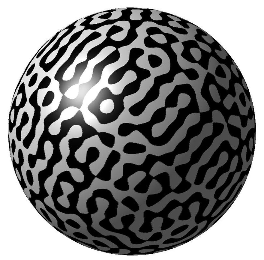
14 250 STEVE ZELDITCH The critical point equation for cos k, x is k sin k, x = 0 and is thus the same as the nodal equation. In particular, the critical point sets are hypersurfaces in this case. There is just one critical value =. Instead of the square torus we could consider R n /L where L R n is a lattice of full rank. Then the joint spectrum becomes the dual lattice L and the eigenfunctions are cos k, x, sin k, x with k L. The real eigenspace H λ = R span{sin k, x, cos k, x : k = λ} is of multiplicity 2 for generic L but has unbounded multiplicity in the case of L = Z n and other rational lattices. In that case, one may take linear combinations of the basic eigenfunctions and study their nodal and critcal point sets. For background, some recent results and further references we refer to [BZ] Spherical harmonics on S 2. The spectral decomposition for the Laplacian is the orthogonal sum of the spaces of spherical harmonics of degree N, (20) L 2 (S 2 )= V N, Δ VN = λ N Id. N=0 The eigenvalues are given by λ S2 N = N(N + ) and the multiplicities are given by m N =2N +. A standard basis is given by the (complex valued) spherical harmonics Ym N which transform by e imθ under rotations preserving the poles. The Ym N are complex valued, so we study the nodal sets of their real and imaginary parts. They are separable, i.e. factor as C N,m Pm N (r) sin(mθ) (resp. cos(mθ) where Pm N is an associated Legendre function. Thus the nodal sets of these special eigenfunctions form a checkerboard pattern that can be explicitly determined from the known behavior of zeros of associated Legendre functions. See the first image in the illustration below. Among the basic spherical harmonics, there are two special ones: the zonal spherical harmonics (i.e. the rotationally invariant harmonics) and the highest weight spherical harmonics. Their nodal sets and intensity plots are graphed in the bottom two images, respectively. Since the zonal spherical harmonics Y0 N on S 2 are real-valued and rotationally invariant, their zero sets consist of a union of circles, i.e. orbits of the S rotation action around the third axis. It is well known that Y0 N(r) = (2N+) 2π P N (cos r), where P N is the Nth Legendre function and the normalizing constant is chosen so that Y0 N L 2 (S 2 ) =, i.e. 4π π/2 0 P N (cos r) 2 dv(r) =, where dv(r) = sin rdr is the polar part of the area form. Thus the circles occur at values of r so that P N (cos r) =0.All zeros of P N (x) are real and it has N zeros in [, ]. It is classical that the zeros r,...,r N of P N (cos r) in(0,π) become uniformly distributed with

15 EIGENFUNCTIONS AND NODAL SETS 25 Figure 3. Examples of the different kinds of spherical harmonics. respect to dr [Sz]. It is also known that P N has N distinct critical points [C, Sz2] and so the critical points of Y0 N is a union of N lattitude circles. We now consider real or imaginary parts of highest weight spherical harmonics YN N. Up to a scalar multiple, Y N(x,x 2,x 2 )=(x + ix 2 ) N as a harmonic polynomial on R 3. It is an example of a Gaussian beams along a closed geodesic γ (such as exist on equators of convex surfaces of revolution). See [R] for background on Gaussian beams on Riemannian manifolds. The real and imaginary parts are of the form PN N (cos r) cos Nθ, PN N(cos r) sin Nθ where P N N(x) is a constant multiple of ( x2 ) N/2 so PN N(cos r) = (sin r)n. The factors sin Nθ,cos Nθ have N zeros on (0, 2π). The Legendre funtions satisfy the recursion relation P l+ l+ = (2l +) x 2 Pl l(x) with P 0 0 = and therefore have no real zeros away from the poles. Thus, the nodal set consists of N circles of longitude with equally spaced intersections with the equator. The critical points are solutions of the pair of equations d dr P N N (r) cos Nθ =0,PN N sin Nθ = 0. Since P N N has no zeros away from the poles, the second equation forces the zeros to occur at zeros of sin Nθ. But then cos Nθ 0 d so the zeros must occur at the zeros of dr P N N (r). The critical points only occur when sin r = 0 or cos r = 0 on (0,π). There are critical points at the poles where YN N vanishes to order N and there is a local maximum at the value r = π 2 of the equator. Thus, Re Y N N has N isolated critical points on the equator and multiple critical points at the poles. We note that Re YN N 2 is a Gaussian bump with peak along the equator in the radial direction. Its radial Gaussian decay implies that it extremely small outside a N 2 tube around the equator. The complement of this tube

16 252 STEVE ZELDITCH is known in physics as the classically forbidden region. We see that the nodal set stretches a long distance into the classically forbidden region. This creates problems for nodal estimates since exponentially small values (in terms of the eigenvalue) are hard to distinguish from zeros. On the other hand, it has only two (highly multiple) critical points away from the equator Random spherical harmonics and chaotic eigenfunctions. The examples above exhibit quite disparate behavior but all are eigenfunctions of quantum integrable systems. We do not review the general results in this case but plan to treat this case in an article in preparation [Z9]. Figure 4 contrasts the nodal set behavior with that of random spherical harmonics (left) and a chaotic billiard domain (the graphics are due to E. J. Heller). 4. Lower bounds on hypersurface areas of nodal sets and level sets in the C case In this section we review the lower bounds on H n (Z ϕλ ) from [CM, SoZ, SoZa, HS, HW]. Here H n (Z ϕλ )= ds Z ϕλ is the Riemannian surface measure, where ds denotes the Riemannian volume element on the nodal set, i.e. the insert iota n dv g of the unit normal into the volume form of (M,g). The main result is: Theorem 4.. Let (M,g) be a C Riemannian manifold. Then there exists a constant C independent of λ such that n Cλ 2 H n (Z ϕλ ). We sketch the proof of Theorem 4. from [SoZ, SoZa]. The starting point is an identity from [SoZ] (inspired by an identity in [Dong]): Proposition 4.2. For any f C 2 (M), (2) ϕ λ (Δ g + λ 2 )fdv g =2 g ϕ λ fds, M Z ϕλ This identity can be used to obtain some rudimentary but non-trivial information on the limit distribution of nodal sets in the C case; see 4.9. For the moment we only use it to study hypersurface measures of nodal sets. When f we obtain Corollary 4.3. (22) λ 2 M ϕ λ dv g =2 g ϕ λ fds, Z ϕλ The lower bound of Theorem 4. follows from the identity in Corollary 4.3 and the following lemma:

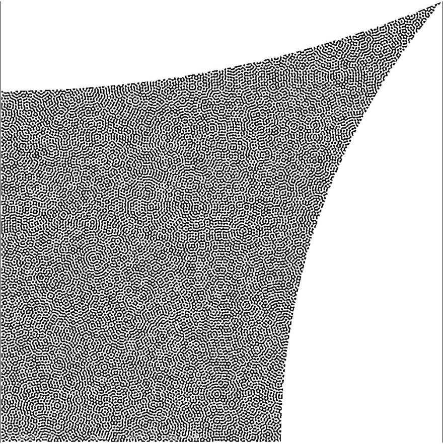
17 EIGENFUNCTIONS AND NODAL SETS 253 Figure 4

18 254 STEVE ZELDITCH Lemma 4.4. If λ>0 then n + (23) g ϕ λ L (M) λ 2 ϕλ L (M) Here, A(λ) B(λ) means that there exists a constant independent of λ so that A(λ) CB(λ). By Lemma 4.4 and Corollary 4.3, we have (24) λ 2 M ϕ λ dv =2 Z λ g ϕ λ g ds 2H n (Z λ ) g ϕ λ L (M) 2H n n + (Z λ ) λ 2 ϕ λ L (M). Thus Theorem 4. follows from the somewhat curious cancellation of ϕ λ L from the two sides of the inequality. 4.. Proof of Proposition 4.2. We begin by recalling the co-area formula: Let f : M R be Lipschitz. Then for any continuous function u on M, Equivalently, M M u(x)dv = R u(x) f dv = ( R f (y) ( f (y) u dv df ) dy. udh n )dy. We refer to dv df as the Leray form on the level set {f = y}. Unlike the Riemannian surface measure ds = dh n it depends on the choice of defining function f. The surface measures are related by dh n = f dv df. For background, see Theorem. of [HL]. There are several ways to prove the identity of Lemma 4.2. One way to see it is that dμ λ := (Δ + λ 2 ) ϕ λ dv = 0 away from {ϕ λ =0}. Hence this distribution is a positive measure supported on Z ϕλ. To determine the coefficient of the surface measure ds we calculate the limit as δ 0ofthe integral f(δ + λ 2 ) ϕ λ dv = f(δ + λ 2 ) ϕ λ dv. M ϕ λ δ Here f C 2 (M) and with no loss of generality we may assume that δ is a regular value of ϕ λ (by Sard s theorem). By the Gauss-Green theorem, f(δ + λ 2 ) ϕ λ dv ϕ λ (Δ + λ 2 )fdv ϕ λ δ ϕ λ δ = (f ν ϕ λ ϕ λ ν f)ds. ϕ λ =δ

19 EIGENFUNCTIONS AND NODAL SETS 255 Here, ν is the outer unit normal and ν derivative. For δ>0, we have is the associated directional (25) ν = ϕ λ ϕ λ on {ϕ λ = δ}, ν = ϕ λ ϕ λ on {ϕ λ = δ}. Letting δ 0 (through the sequence of regular values) we get f(δ+λ 2 ) ϕ λ dv = lim f(δ+λ 2 ) ϕ λ dv = lim f ν ϕ λ ds. M δ 0 ϕ λ δ δ 0 ϕ λ =δ Since ϕ λ = ±ϕ λ on {ϕ λ = ±δ} and by (25), we see that M f(δ + λ2 ) ϕ λ dv = lim δ 0 ϕ λ =δ f ϕ λ ϕ λ ϕ λ ds = lim δ 0 ± ϕ λ =±δ f ϕ λ ds = 2 Z ϕλ f ϕ λ ds. The Gauss-Green formula and limit are justified by the fact that the singular set Σ ϕλ has codimension two. We refer to [SoZ] for further details Proof of Lemma 4.4. Proof. The main idea is to construct a designer reproducing kernel for ϕ λ of the form (26) ˆρ(λ Δ g )f = ρ(t)e itλ e it Δ g f dt, with ρ C0 (R). It has the spectral expansion, (27) χ λ f = ˆρ(λ λ j )E j f, j=0 where E j f is the projection of f onto the λ j - eigenspace of Δ g. Then (26) reproduces ϕ λ if ˆρ(0) =. We denote the kernel of χ λ by K λ (x, y), i.e. χ λ f(x) = K λ (x, y)f(y)dv (y), (f C(M)). M Assuming ˆρ(0) =, then K λ (x, y)ϕ λ (y)dv (y) =ϕ λ (x). M To obtain Lemma 4.4, we choose ρ so that the reproducing kernel K λ (x, y) is uniformly bounded by λ n 2 on the diagonal as λ +. It suffices to choose ρ so that ρ(t) =0for t / [ε/2,ε], with ε>0 less than the injectivity radius of (M,g), then it is proved in Lemma 5..3 of [Sog3] that (28) K λ (x, y) =λ n 2 aλ (x, y)e iλr(x,y),

20 256 STEVE ZELDITCH where a λ (x, y) is bounded with bounded derivatives in (x, y) and where r(x, y) is the Riemannian distance between points. This WKB formula for K λ (x, y) is known as a parametrix. It follows from (28) that (29) n + g K λ (x, y) Cλ 2, and therefore, sup x M g χ λ f(x) = sup x f(y) g K λ (x, y) dv g K λ (x, y) L (M M) f L n + Cλ 2 f L. To complete the proof of Lemma 4.4, we set f = ϕ λ and use that χ λ ϕ λ = ϕ λ. We view K λ (x, y) as a designer reproducing kernel, because it is much smaller on the diagonal than kernels of the spectral projection operators E [λ,λ+] = j:λ j [λ,λ+] E j. The restriction on the support of ρ removes the big singularity on the diagonal at t = 0. As discussed in [SoZa], it is possible to use this kernel because we only need it to reproduce one eigenfunction and not a whole spectral interval of eigenfunctions Modifications. After an initial modification in [HW], an interesting application of Proposition 4.2 was used in [HS] to prove Theorem 4.5. [HS] For any C compact Riemannian manifold, the L 2 -normalized eigenfunctions satisfy H n (Z ϕλ ) Cλ ϕ λ 2 L. They first apply the Schwarz inequality to get ( ) /2 (30) λ 2 ϕ λ dv g 2(H n (Z ϕλ )) /2 g ϕ λ 2 ds. M Z ϕλ They then use the test function (3) f = ( +λ 2 ϕ 2 λ + gϕ λ 2 g in Proposition 4.2 to show that (32) g ϕ λ 2 ds λ 3. Z ϕλ A simpler approach to the last step was suggested by W. Minicozzi, who pointed out that the result also follows from the identity (33) 2 g e λ 2 ( ) ds g = sgn(ϕ λ ) div g g e λ g e λ dvg. Z λ M ) 2

21 EIGENFUNCTIONS AND NODAL SETS 257 This approach is used in [Ar] to generalize the nodal bounds to Dirichlet and Neumann eigenfunctions of bounded domains. Theorem 4.5 shows that Yau s conjectured lower bound would follow for a sequence of eigenfunctions satisfying ϕ λ L C>0for some positive constant C More general identities. It is possible to further generalize the identity of Proposition 4.2 and we pause to record an obvious one. For any function χ, we have Δχ(ϕ) =χ (ϕ) ϕ 2 λ 2 χ (ϕ)ϕ. We then take χ to be the meromorphic family of homogeneous distribution x s +. We recall that for Re a>, x a, x 0 x a + := 0, x < 0. The family extends to a C as a meromorphic family of distributions with simple poles at a =, 2,..., k,... using the equation d dx x +s = sx s + to extend it one unit strip at a time. One can convert x s + to the holomorphic family χ α x α + + = Γ(α +), with χ k + = δ(k ) 0. The identity we used above belongs to the family, (34) (Δ + sλ 2 )ϕ s + = s(s ) ϕ 2 ϕ s 2 +. Here ϕ s + = ϕ x s + has poles at s =, 2,. The calculation in (2) used ϕ but is equivalent to using (34) when s =. Then ϕ s 2 + has a pole when ds ϕ ds Z ϕλ ; it is cancelled by the factor s s = with residue δ 0 (ϕ) = and we obtain (2). This calculation is formal because the pullback formulae are only valid when dϕ 0 when ϕ = 0, but as above they can be justified because the singular set has codimension 2. The right side also has a pole at s = 0 and we get Δϕ 0 + = ϕ 2 δ (ϕ), which is equivalent to the divergence identity above. There are further poles at s =, 2,... but they now occur on both sides of the formulae. It is possible that they have further uses. Such identities appear to be related to the Bernstein-Kashiwara theorem that for any real analytic function f one may meromorphically extend f+ s to C by constructing a family P s (D) of differential operators with analytic coefficients and a meromorphic function b(s) so that P s (D)f s+ = b(s)f s. In the case f = ϕ λ, the operator ϕ 2 (Δ + sλ 2 ) accomplishes something like this, although it does not have analytic coefficients due to poles at the critical points of ϕ.

22 258 STEVE ZELDITCH 4.5. Other level sets. These results generalize easily to any level set Nϕ c λ := {ϕ λ = c}. Let sgn(x) = x x. Proposition 4.6. For any C Riemannian manifold, and any f C(M) we have, (35) M f(δ+λ 2 ) ϕ λ c dv +λ 2 c fsgn(ϕ λ c)dv =2 N c ϕ λ f ϕ λ ds. This identity has similar implications for H n (N c ϕ λ ) and for the equidistribution of level sets. Note that if c>sup ϕ λ (x) then indeed both sides are zero. Corollary 4.7. For c R λ 2 ϕ λ dv = ϕ λ ds λ 2 Vol(M) /2. ϕ λ c Nϕ c λ Consequently, if c>0 H n (Nϕ c λ )+H n (Nϕ c n+ 2 λ ) C g λ 2 ϕ λ dv. ϕ λ c The Corollary follows by integrating Δ by parts, and by using the identity, M ϕ λ c + c sgn(ϕ λ c) dv = ϕ λ >c ϕ λdv ϕ λ <c ϕ λdv (36) = 2 ϕ λ >c ϕ λdv, since 0 = M ϕ λdv = ϕ λ >c ϕ λdv + ϕ λ <c ϕ λdv Examples. The lower bound of Theorem 4. is far from the lower bound conjectured by Yau, which by Theorem 2. is correct at least in the real analytic case. In this section we go over the model examples to understand why the methds are not always getting sharp results Flat tori. We have, sin k, x 2 = cos 2 k, x k 2. Since cos k, x = when sin k, x = 0 the integral is simply k times the surface volume of the nodal set, which is known to be of size k. Also, we have T sin k, x dx C. Thus, our method gives the sharp lower bound H n (Z ϕλ ) Cλ in this example. So the upper bound is achieved in this example. Also, we have T sin k, x dx C. Thus, our method gives the sharp lower bound H n (Z ϕλ ) Cλ in this example. Since cos k, x = when sin k, x =0 the integral is simply k times the surface volume of the nodal set, which is known to be of size k.

23 EIGENFUNCTIONS AND NODAL SETS Spherical harmonics on S 2. The L of Y0 N norm can be derived from the asymptotics of Legendre polynomials P N (cos θ) = ( 2(πN sin θ) 2 cos (N + 2 )θ π ) + O(N 3/2 ) 4 where the remainder is uniform on any interval ɛ<θ<π ɛ. Wehave (2N +) π/2 Y0 N L =4π P N (cos r) dv(r) C 0 > 0, 2π 0 i.e. the L norm is asymptotically a positive constant. Hence Z Y Y N 0 N ds 0 C 0 N 2. In this example Y0 N L = N 3 2 saturates the sup norm bound. The length of the nodal line of Y0 N is of order λ, as one sees from the rotational invariance and by the fact that P N has N zeros. The defect in the argument is that the bound Y0 N L = N 3 2 is only obtained on the nodal components near the poles, where each component has length N. Gaussian beams Gaussian beams are Gaussian shaped lumps which are concentrated on λ n 2 tubes T λ (γ) around closed geodesics and have height λ 4. 2 We note that their L norms decrease like λ (n ) 4, i.e. they saturate the L p bounds of [Sog] for small p. In such cases we have Z ϕλ ϕ λ ds λ 2 n 2 ϕ λ L λ 4. Gaussian beams are minimizers of the L norm among L 2 -normalized eigenfunctions of Riemannian manifolds. Also, the gradient bound ϕ λ L = O(λ n+ 2 ) is far off for Gaussian beams, the correct upper n + bound being λ 4. If we use these estimates on ϕ λ L and ϕ λ L, our method gives H n n (Z ϕλ ) Cλ 2, while λ is the correct lower bound for Gaussian beams in the case of surfaces of revolution (or any real analytic case). The defect is again that the gradient estimate is achieved only very close to the closed geodesic of the Gaussian beam. Outside of the tube T λ (γ) of radius λ 2 around the geodesic, the Gaussian beam and all 2 of its derivatives decay like e λd2 where d is the distance to the geodesic. Hence Z ϕλ ϕ λ ds Z ϕλ T λ (γ) ϕ λ ds. Applying the gradient bound 2 for Gaussian beams to the latter integral gives H n (Z ϕλ T λ (γ)) 2 n Cλ 2, which is sharp since the intersection Z ϕλ T λ (γ) cuts across 2 γ in λ equally spaced points (as one sees from the Gaussian beam approximation) Non-scarring of nodal sets on (M,g) with ergodic geodesic flow. The identity of Lemma 4.2 for general f C 2 (M) can be used to investigate the equidistribution of nodal sets equipped with the surface measure ϕ λ ds. We denote the normalized measure by λ 2 ϕ λj ds Zϕλ.

24 260 STEVE ZELDITCH We first prove a rather simple (unpublished) result on nodal sets when the geodesic flow of (M,g) is ergodic. Since there exist many expositions of quantum ergodic eigenfunctions, we only briefly recall the main facts and definitions and refer to [Z5, Z6] for further background. Quantum ergodicity concerns the semi-classical (large λ) asymptotics of eigenfunctions in the case where the geodesic flow G t of (M,g) is ergodic. We recall that the geodesic flow is the Hamiltonian flow of the Hamiltonian H(x, ξ) = ξ 2 g (the length squared) and that ergodicity means that the only G t -invariant subsets of the unit cosphere bundle S M have either full Liouville measure or zero Liouville measure (Liouville measure is the natural measure on the level set H = induced by the symplectic volume measure of T M). We will say that a sequence {ϕ jk } of L 2 -normalized eigenfunctions is quantum ergodic if (37) Aϕ jk,ϕ jk μ(s σ A dμ, A Ψ 0 (M). M) S M Here, Ψ s (M) denotes the space of pseudodifferential operators of order s, σ A denotes the principal symbol of A, and dμ denotes Liouville measure on the unit cosphere bundle S M of (M,g). More generally, we denote by dμ r the (surface) Liouville measure on Br M, defined by (38) dμ r = ωm on Br M. d ξ g We also denote by α the canonical action -form of T M. The main result is that there exists a subsequence {ϕ jk } of eigenfunctions whose indices j k have counting density one for which ρ jk (A) := Aϕ jk,ϕ jk ω(a) (where as above ω(a) = μ(s M) S M σ Adμ is the normalized Liouville average of σ A ). The key quantities to study are the quantum variances (39) V A (λ) := Aϕ j,ϕ j ω(a) 2. N(λ) j:λ j λ The following result is the culmination of the results in [Sh., Z, CV, ZZw, GL]. Theorem 4.8. Let (M,g) be a compact Riemannian manifold (possibly with boundary), and let {λ j,ϕ j } be the spectral data of its Laplacian Δ. Then the geodesic flow G t is ergodic on (S M,dμ) if and only if, for every A Ψ o (M), we have: () lim λ V A (λ) =0. (2) ( ɛ)( δ) lim sup λ N(λ) j k:λ j,λ k λ (Aϕ j,ϕ k ) 2 <ɛ λ j λ k <δ

25 EIGENFUNCTIONS AND NODAL SETS 26 Since all the terms in () are positive, no cancellation is possible, hence () is equivalent to the existence of a subset S Nof density one such that Q S := {dφ k : k S}has only ω as a weak* limit point. We now consider nodal sets of quantum ergodic eigenfunctions. The following result says that if we equip nodal sets with the measure ϕ λ 2 λj ds, j then nodal sets cannot scar, i.e. concentrate singularly as λ j. Proposition 4.9. Suppose that {ϕ λj } is a quantum ergodic sequence. Then any weak limit of { ϕ λ 2 λj ds} must be absolutely continuous with j respect to dv g. (In fact this will be improved below in Corollary 4.3). The first point is the following Lemma 4.0. The weak * limits of the sequence {λ 2 ϕ λj ds Zϕλ } of bounded positive measures are the same as the weak * limits of { ϕ λj } (against f C(M).) We let f C 2 (M) and multiply the identity of Proposition 4.2 by λ 2. We then integrate by parts to put Δ on f. This shows that for f C 2 (M), we have f ϕ λ dv = λ Z 2 f λ ds + O(λ 2 ). ϕλ M Letting f =, we see that the family of measures {λ 2 ϕ λj 2 δ(ϕ λj )} is bounded. By uniform approximation of f C(M) by elements of C 2 (M), we see that the weak* limit formula extends to C(M). Lemma 4.. Suppose that {ϕ λj } is a quantum ergodic sequence. Then any weak limit of { ϕ λj ds} must be absolutely continuous with respect to dv. We recall that a sequence of measures μ n converges weak * to μ if M fdμ n fdμ for all continuous f. A basic fact about weak * convergence of measures is that fdμ n fdμ for all f C(M) implies that μ n (E) μ(e) for all sets E with μ( E) = 0 (Portmanteau theorem). We also recall that a sequence of eigenfunctions is called quantum ergodic (in the base) if (40) f ϕ λj 2 dv fdv. Vol(M) M In other words, ϕ 2 λ in the weak * topology, i.e. the vague topology on measures. We now prove Lemma 4.. Proof. Suppose that ϕ λjk dv dμ and assume that dμ = cdv + dν where dν is singular with respect to dv. Let Σ = supp ν, and let σ = μ(σ) = ν(σ). Let T ɛ be the ɛ-tube around Σ. Then lim ϕ λjk dv = cv ol(t ɛ )+ν(σ) = σ + O(ɛ). k T ɛ

26 262 STEVE ZELDITCH But for any set Ω M, Ω ϕ λ j dv Vol(Ω) Ω ϕ λ j 2 dv. Hence if Vol( Ω) = 0, lim sup j Ω ϕ λ j dv Vol(Ω). Letting Ω = T ɛ (Σ) we get σ+o(ɛ) Vol(T ɛ (Σ)) = O(ɛ) since lim k T ɛ ϕ λjk 2 dv = Vol(T ɛ )=O(ɛ). Letting ɛ 0 gives a contradiction. Of course, it is possible that the only weak* limit is zero A stronger non-scarring result. G. Rivière [Ri] pointed out some improvements to Proposition 4.9. Proposition 4.2. Suppose that {ϕ jk } is a sequence of L 2 normalized eigenfunctions satisfying the following weak quantum ergodic condition: (WQE): ϕ jk 2 dv g ρdv g weak, with ρ L (M,dV g ). Suppose also that ϕ jk dv g dμ, where μ is a probability measure on M. Then μ = FdV g with F L (M,dV g ). In fact, the same is true for weak limits of ϕ jk p dv g for any p<2, but we only treat the case p =. Proof. If f C(M) then f ϕ jk dv g ( f 2 ϕjk ) f 2 dvg M Let k and we get M M M fdμ ρ L f L. f ϕ jk 2 2 dv g f 2. L Hence f fdμ is a continuous linear functional on L and must have the form μ = FdV g where F ρ. Corollary 4.3. Suppose that {ϕ λj } is a quantum ergodic sequence. Then any weak limit of { ϕ λ 2 λj ds} must be of the form FdV g with j F. 4.. Weak* limits for L quantum ergodic sequences. To our knowledge, the question whether the limit (4.8) holds f L when (M,g) has ergodic geodesic flow has not been studied. It is equivalent to strengthening the Portmanteau statement to all measurable sets E, and is equivalent to the statement that {ϕ 2 λ j } weakly in L. We call such sequences L quantum ergodic on the base. The term on the base refers to the fact that we only demand quantum ergodicity for the projections of the microlocal lifts to the base M. For instance, the exponential eigenfunctions of flat tori are L quantum ergodic in this sense.