Introduction to Marine Hydrodynamics

Transcription

1 Introduction to Marine Hydrodynamics (NA35) Department of Naval Architecture and Ocean Engineering School of Naval Architecture, Ocean & Civil Engineering Shanghai Jiao Tong University

2 Chapter 7 Water Waves

3 For Airy wave, we need to determine three parameters, (A, k, ω). In fact, only two of them, (A, k), need to be determined, since a dispersion relation exists, that will be introduced soon later in this section. Acoskx t 1. Airy wave is a -dimensional cosine function, known as cosine wave, sine wave or linear sinusoidal wave. A -- wave amplitude; H = A -- wave height. λ -- wave length, the distance between two adjacent crests or troughs.

4 . k : the wave number Let t = 0, Airy wave becomes simply a cosine function of x. Acos kx kx n (n is an integer) For n = 1, it corresponds one wave form, that is, x =λ, therefore k K k = wavenumber = π/ [L -1 ]

5 3. ω : circular frequency Let x = 0, Airy wave becomes a cosine function of t. Acost t n (n is an integer) For n = 1, it corresponds one period, t = T = 1/f, therefore f T where T 1 f T = frequency = π/t [T -1 ], e.g. rad/sec

6 4. Phase velocity / Celerity ( c or V p ): wave form moving velocity Let s look at a fixed position in space where at an instant a crest located at. Then the crest moves forward. The duration until another crest arrives at that point is just one wave period. During this period, we can see the wave form moves forward just one wave length. So, velocity the wave form advances is cv p y T MWL A Vp (x,t) = y x h

7 Airy wave is also known as sinusoidal wave. It is expressed as Acoskx t Acos k x t Acos k x ct k where k T T c Phase velocity, wave length, wave period, wave frequency, circular frequency and wave number related with each other as follows: c T k

8 5. Dispersion relation: relation between circular frequency and wave number. Velocity potential ga sin Now, substituting the velocity potential in the linearized free surface condition, it yields kx t cosh k y h cosh Free surface condition g 0 (on y = 0) y t That is the dispersion relation. cosh kh gk sinh kh 0 sinh kh gk gk tanh kh cosh kh kh

9 If we want to calculate the wave number from a given water depth and a given circular frequency, it is difficult to derive an explicit expression. Instead, we can write the dispersion relation in a form below and try to find the intersection of two functions (curves), the left hand side function and the right side function of the equation. h C kh kh g C kh tanh tanh kh C kh 1 tanh kh 1/5 1 kh =f(c) 3 kh

10 Some characteristics of the related hyperbolic functions f deep water shallow water kh 3 kh 1 f kh 0 tanh 1 kh f f f 1 3 y y y cosh cosh sinh k y h cosh kh k y h sinh kh k y h sinh kh e e ky ky ky e kh y h

11 Equating function f 1 (kh) and function f (kh), we can get solution, kh, of the dispersion relation. Geometrically, the solution corresponds the intersection of the two curves of f 1 (kh) and f (kh). C f1 kh kh f kh tanh kh where C g h kh if kh 1, or, h (shallow water) kh sinh kh 1 e tanh kh 1 if kh 3, or, h kh cosh kh 1 e (deep water) (tanh )

12 For a given water depth h, wave dispersion relation gives a correspondence between the wave circular frequency ω and the wave number k. circular frequency (ω) Since c be written as k wave number (k) and k, the dispersion relation can c g h tanh k Therefore, the dispersion relation also give the correspondence between phase velocity (c) and wave length (λ), provided water depth h is given. phase velocity (c) wave length (λ)

13 tanh kh 1 Deep water waves: If kh 3, or, h 3, approximately h, then it results the deep water dispersion relation gk T g c d g k g Therefore, Since h 1 k; T; c, deep water waves are also called short waves..

14 Shallow water waves: If kh 1, or, h 1, that is, h, generally, if h 5, water depth can be considered small enough. Since ghk tanh kh T kh it results shallow water dispersion relation. gh cs gh Therefore, length any more. For h 1 5 k, T, and c does not relate to wave, shallow water waves are also known as long waves.

15 1 h 1 5 h Generally for water depth in between ( or ): 0.08 c h c tanhkh h tanh kh tanh, tanh c c kh h d s h

16 For a fixed water depth, since cs gh is a constant, phase velocity c will decrease with wave lengthλ. That is, longer waves travel faster, and shorter waves travel slower. For waves with fixed wave length, since cd is a constant, phase velocity c will increase with the water depth h. That is, deep water waves travel faster, and shallow water waves travel slower. g h

17 6. Velocity field From velocity potential of the wave flows and dispersion relation, velocity field of the wave flows can be readily derived. ga cosh k y h sin kx t, cosh kh Agk cosh k y h u coskx t x cosh kh cosh ky h A coskx t sinh kh Agk sinh k y h v sin kx t y cosh kh sinh k y h A sin kx t sinh kh gk tanh kh

18 On y = 0 : 1 U 0 A tanh kh kx t cos, V A kx t 0 sin then, velocity can be written relative to that on y = 0, it gives t u U 0 cosh k y h cosh kh, v V 0 sinh k y h sinh kh v V 0 u U 0

19 Shanghai Jiao Tong University For deep water waves, kh 3, we have u U 0 cosh k y h cosh kh e ky, v V 0 sinh k y h sinh kh e ky g k g k

20 u U Shanghai Jiao Tong University For shallow water waves, 0 cosh k y h cosh kh kh 1 1, 0, we have v sinh k y h y 1 V sinh kh h A u kx t kh g h cos, v A 1 sinkx t y h

21 Characteristics of Airy waves deep water shallow water kh 3 kh 1 dispersion relation velocity c d gk g g k u ky e U v V 0 0 e ky cs u U v V 0 ghk 0 gh 1 1 y h

22 7. Particle orbit At time t, fluid particle P takes the position (x P (t), y P (t)), and if we denote its mean position is xp, yp and P(x p,y p ) x P() t xp x P() t y () t y y () t P P P Since velocity is a time derivative of position, that is, x, y,,,, (x,y ) dx u x y t u x y t P up ux, y, t x y dt x y remaining the main first term and integrating the equation, it gives cosh k y h x P x ux, y, tdt x A coskx tdt sinh kh cosh ky h x A sin kx t sinh kh

23 7. Particle orbit At time t, fluid particle P takes the position (x P (t), y P (t)), and if we denote its mean position xp, yp and P(x p,y p ) x P() t xp x P() t y () t y y () t P P P Since velocity is a time derivative of position, that is, x, y,,,, (x,y ) dx u x y t u x y t P up ux, y, t x y dt x y remaining the main first term and integrating the equation, it gives cosh k y h x P x ux, y, tdt x A coskx tdt sinh kh cosh ky h x A sin kx t sinh kh

24 Similarly,,, v x, y, t dy v x y t P vp vx, y, t x y dt x y keeping the first term only and integrating the equation, it results sinh k y h yp y vx, y, tdt y A sinkx tdt sinh kh sinh ky h y A coskx t sinh kh Specifically, on the mean free surface,, the unknown wave elevation is obtained. y 0 y Acoskx t P

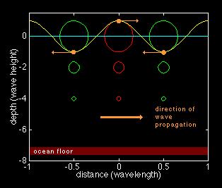
25 Then, the particle orbit of particle P is obtained. where a A P 1 x x y y P cosh a k y h sinh kh b, b A sinh k y h sinh kh Particle orbits are ellipses. Both major axis and minor axis decrease with the increase of the depth below the free surface.

26 a b Ae Accordingly particle orbits become circles. The radius is getting smaller with the increase of depth from the free surface. On the free surface, the radius is just equal to the wave amplitude. kh 1 For deep water wave,, major and minor axes become equal ky

27

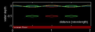
28 For shallow water waves,, the major and minor axes are a A kh const, kh 1 The particle orbits are ellipses. Major axis is horizontal and keeps constant, while the minor axis is vertical and decreases linearly with the depth from the free surface: on free surface, y = 0, it equals the wave amplitude, and on sea bottom, y = -h, it reduces to zero. b A1 y h

29

30 8. Pressure field According to the linearized dynamic condition (Bernoulli s equation), the pressure is evaluated as follows p pa gy t cosh k y h ga coskx t gy cosh kh cosh k y h g gy cosh kh

31 kh 1 cosh k y h cosh kh For deep water wave,, since we have approximation pressure is approximately written as ky p pa g e y V p gh that is, the dynamic pressure, the exponential part, decays with the increase of depth from free surface. Below half wave length, it could be reasonably neglected, where static pressure dominates. e ky V p (kh >> 1) p (kh << 1) p p d p s p d

32 For shallow water wave,, since we have approximation on the left, pressure distribution is approximated as p p g y a kh 1 cosh k y cosh kh h 1 that is, the pressure is very similar to static pressure distribution. The only difference is that the depth is measured from the instantaneous wave surface. V p gh V p (kh >> 1) p (kh << 1) p p d p s p d

33 Eg. 1 For an Airy wave, it is given that amplitude A = 0.3 m, wave period T = s, calculate its circular frequency, wave number, phase velocity, wave length and the maximum wave slope. Solution: Circular frequency: 3.14 s T 1 Wave number: gk 3.14 k g m 1 Phase velocity: c 3.14 k m/s

34 Wave length: m k Wave elevation: Acoskx t x 0.3 cos t x cos 1.01x 3.14t Wave slope: tg Ak sin kx t The maximum wave slope angle: tg max max o

35 Eg. A boat on a water wave is rolling at a rate of 30 cycles per minute. The sea is assumed deep enough. Calculate the wave length L, circular frequency ω, wave number k and the phase velocity c. Solution: Since the boat is not traveling, its rolling is assumed to be caused by an incident water waves. Then, wave period: T circular frequency: wave number: k 1 min ( s ) 30 T g 3.14(1/ s) wave length: L 6.6( m) k phase velocity: L C 3.13( m / s) T

36 Eg. 3 Consider two fluid layers, the upper fluid with densityρ 1, depth h 1, the lower fluid with densityρ, depth h. Two fluids are bounded by uppermost and lowest horizontal rigid walls. Determine phase velocity for the wave at the separating surface of the two layers with wave number k. Solution: Take origin at the mean separating surface, x- axis horizontal and y-axis vertical, upward positive.then velocity potentials of the wave in each layers are respectively as follows, in the upper layer ga cosh k yh sin cosh sin cosh kh in the lower layer kx t C k y h kx t ga cosh k y h sin cosh sin cosh kh kx t D k y h kx t y x

37 On the interface of the upper and lower fluid layers, pressure and velocity should coincide with each other. According to Bernoulli s equation, we have p p gy 0, gy 0 t t y p p On the interface,, pressure coincidence requires,, i.e. g g ( y 0) t t 1 g t t y 0

38 Next, velocity coincidence. On the interface, y-components of the upper and lower velocities should be equal, that is y y ( y 0) kc sinh k h sin kx t kd sinh kh sin kx t Thus, Csinh kh Dsinh kh From the linear kinematic condition of Airy wave, we have ( y 0) y y t

39 Therefore, 1 ( y 0) y g t t kdsinh khsin kx t Ccosh k h Dcosh kh g kdg sinh kh D cosh kh C cosh kh sin kx t

40 From above expression, finally we can get phase velocity formula. c k k Dg sinh kh k Dcosh kh C cosh kh g cosh kh C cosh kh k sinh kh D sinh kh g k tanh kh tanh kh End of Eg. 3.