Gestion de la production. Book: Linear Programming, Vasek Chvatal, McGill University, W.H. Freeman and Company, New York, USA

Transcription

1 Gestion de la production Book: Linear Programming, Vasek Chvatal, McGill University, W.H. Freeman and Company, New York, USA 1

2 Contents 1 Integer Linear Programming Definitions and notations Solvers Example LibreOffice Solver Branch-And-Bound Algorithm Minimization of concave piece-wise affine functions Constraints with absolute value expressions Soft Constraints, Big-M constraints, Alldiff constraints Boolean expressions ILP Relaxations Lagrangian Relaxation

3 1 Integer Linear Programming 1.1 Definitions and notations An integer linear program is a linear program with the additional constraint that the variables are required to be integer. Z(ILP)= min c x (1) Ax b (2) x Z + (3) where A R m n, b R m, c R n. c 1 a 11 a a 1n b 1 c 2 INPUT DATA : A = a 21 a a 2n b = b 2... c = a m1 a m2... a mn b m... c n x 2 VARIABLES : x = x n Equivalent way an writing an ILP: Z(ILP)= min c j x j (4) a ij x j b i i = 1,..., m (5) x j Z + j = 1,..., n (6) Z(LP) is a valid bound for Z(ILP): lower bound in case of minimization upper bound in case of maximization Definition: y R, the integer part of y is y =max integer q : q y if c j Z ( j = 1,..., n): for minimization Z(LP ) + 1 is a valid lower bound for Z(ILP) for maximization Z(LP ) is a valid upper bound for Z(ILP) Example: A = [ 50 ] b = [ ] c = [ ] x = [ x1 ] Z(ILP) = max x x x x x 2 4, x 2 Z + the optimal LP solution value is Z(LP)= Z(LP) is an upper bound for Z(ILP) upper bound =

4 x 2 (0, ) x 2 = Z(LP)= (0, 2) f(x) = [ ] Z(ILP)=5 x 1 = (5, 0) Z(LP ) is an upper bound for Z(ILP) upper bound =5 ] the optimal LP solution x LP = [ the optimal solution value is Z(ILP)=5 [ ] 5 the optimal solution x = 0 very far from the optimal integer solution Definition Mixed Integer Linear Program (MILP) An ILP when some variables are restricted to be integer and some are not, the problem is called: mixed integer linear program. Z(MILP)= min c x (7) Ax b (8) x 0 (9) x j Z + j = 1,..., p (10) Definition Binary program (BP) An ILP where the integer variables are restricted to be 0 or 1 (it comes up surprisingly often). Such problems are called pure (mixed) 0 1 linear programs or pure (mixed) binary integer linear programs. Z(BP)= min c x (11) Ax b (12) x {0, 1} (13) 4

5 Modeling Potential Modeling with integer variables is useful in a wide variety of applications and in many financial application/problems: model managerial decisions select among different resources allocate scarce resources manage portfolios and projects model fixed costs model logical requirements (boolean conditions) many others Solvers Many SOLVERs are available to direct tackle ILP problems. Prototyping: EXCEL Libre Office Commercial solvers: IBM ILOG CPLEX GUROBI XPRESS Open source solvers: SCIP CBC GLPK LPSOLVE Problems with more than a few thousand variables are often not possible to solve unless they show a specific exploitable structure. They implement Exact Algorithms based on the following techniques: Branch and Bound Cutting planes Branch and Cut Branch and Price A combination of the above methods 5

6 max f(x) Feasible D(LP) solutions Optimal LP solution value Z(LP)=Z(D(LP)) Upper Bound Feasible LP solutions Optimal solution value Z(ILP) Feasible integer solution value Z( x) Lower Bound Feasible integer solution value Z( x) Lower Bound Feasible integer solution value Z( x) Upper Bound Feasible integer solution value Z( x) Upper Bound Optimal solution value Z(ILP) Feasible LP solutions Optimal LP solution value Z(LP)=Z(D(LP)) Lower Bound Feasible D(LP) solutions min f(x) Relaxations and feasible solutions (for maximization and minimization problems) 1.3 Example Example 1 Suppose we wish to invest 19,000 e and we have four investment opportunities: 1 investment of 6,700 e and has a net present value of 8,000 e 2 investment of 10,000 e and has a net present value of 11,000 e 6

7 3 investment of 5,500 e and has a net present value of 6,000 e 4 investment of 3,400 e and has a net present value of 4,000 e Into which investments should we place our money so as to maximize our total present value? problems are called capital budgeting problems. Such Decision variables: { 1 if investment j is made (j = 1,..., 4) x j = 0 otherwise max 8, , 000x 2 + 6, 000x 3 + 4, 000x 4 (14) 6, , 000x x 3 + 3, 400x 4 19, 000 (15) Ignoring integrality constraints: the optimal linear programming solution is: the optimal linear programming solution is: =1, x 2 =0.89, x 3 = 0, x 4 = 1 the optimal LP solution value is 21,790 e this solution is not integral rounding x 2 down to 0 gives a feasible integer solution of value of 12,000 e the optimal solution is: =0, x 2 =1, x 3 = 1, x 4 = 1 the optimal solution value is 21,000 e There are a number of additional constraints we can add: Only a maximum of two investments can be made + x 2 + x 3 + x 4 2 x i {0, 1} i = 1, 2, 3, 4 (16) If investment 2 is made, then investment 4 must also be made (if investment 4 is not made then either 2 is made) x 2 x 4 0 x 2 x OK 1 1 OK 0 1 OK 1 0 NOT OK If investment 1 is made, then investment 3 cannot be made (if investment 3 is made then 1 cannot be made) + x 3 1 x OK 0 1 OK 1 0 OK 1 1 NOT OK the optimal solution is: =0, x 2 =1, x 3 = 0, x 4 = 1 the optimal solution value is 15,000 e 7

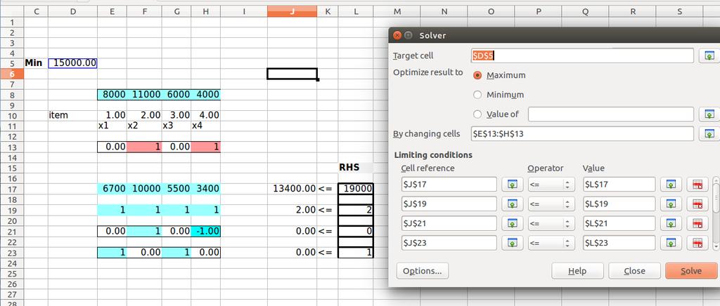
8 1.4 LibreOffice Solver Step-by-step description of the solution of Example 1 using the solver provided by LibreOffice the spreadsheet of the model is presented by the following figure the blue cells represent the input data of the model The model is composed by three parts the variables represented by cells E13,F13,G13,H13 the objective function represented by cell D5 the constraints represented by rows 17,19,21, 23. the first two constraints are represented in the figures the solution of the model is computed using the solver 8

9 the variables are constraint to have binary values as shown in the figure before solving the model is it necessary to set the options pressing the bottom solve you get the optimal solution and the optimal solution value 9

10 10

11 1.5 Branch-And-Bound Algorithm Branch and bound has been the most effective technique for solving MILPs in the following forty years or so (it was proposed in 1960 by Land and Dong). It is based on dividing the problem into a number of smaller problems (branching) and evaluating their quality based on solving the underlying linear programs (bounding). However, in the last ten years, cutting planes have made a resurgence and are now efficiently combined with branch and bound into an overall procedure called branch and cut (this term was coined by in 1987 by Padberg and Rinaldi). The goal is to solve an integer linear program (ILP): Z(ILP)= min c j x j (17) a ij x j b i i = 1,..., m (18) x j Z + j = 1,..., n (19) where matrix A R m n, m-vector b R m, n-vector c R n. The technique can be extended to MILP. Bounding : the engine of the branch and bound algorithm is the solution of the Linear Programming Relaxation of the ILP: Z(LP)= min c j x j (20) a ij x j b i i = 1,..., m (21) x j 0 j = 1,..., n (22) 11

12 The best known (and most successful) methods for solving LPs is the simplex algorithm. Rounding the solution of the LP will not in general give the optimal solution of the ILP. Since the the LP is less constrained than an ILP, the following are immediate: The optimal objective value for the LP is less than or equal to the optimal objective for the ILP If the LP is infeasible, then so is ILP If the optimal solution x of the LP satisfies x i integer for i = 1,..., n, then x is also optimal for the ILP Otherwise, it gives a bound on the optimal value of the ILP Notation and data structure The branch-and-bound algorithm keeps a list of linear programming problems obtained by relaxing the integrality requirements on the variables and imposing constraints such as: x j u j x j l j Each such linear program corresponds to a node of the branch-and-bound tree. For a node N i, let Z(N i ) denote the optimal solution value of the corresponding linear program. Let L denote the list of nodes that must still be solved. Let Z B denote a valid bound on the optimum value (initially, the bound Z B can be derived from a heuristic solution of MILP, or it can be set to + (- ) in case of maximization). Pseudo code of the algorithm (minimization) Step 0 Initialize L = LP, Z B = +, x =. Step 1 Terminate? If L =, the solution x is optimal. Step 2 Select node Choose and delete a problem N i from L. Step 3 Bound Solve N i. If it is infeasible, go to Step 1. Else, let x i be its solution and Z(N i ) its objective value. Step 4 Prune If Z(N i ) Z B, go to Step 1. If x i is not feasible for ILP, go to Step 5. If x i is feasible for ILP, let Z B = Z(N i ), x = x i. Delete from L all problems with Z(N j ) Z B. Go to Step 1. Step 5 Branch From N i, construct linear programs Ni 1,..., N i k with smaller feasible regions whose union contains all the feasible solutions of (MILP) in N i. Add Ni 1,..., N i k to L and go to Step 1. 12

13 Pseudo code of the algorithm (maximization) All the steps remains unchanged except: Step 0 Initialize L = ILP, Z B = -, x =. Step 4 Prune If Z(N i ) Z B, go to Step 1. If x i is not feasible for MILP, go to Step 5. If x i is feasible for ILP, let Z B = Z(N i ), x = x i. Delete from L all problems with Z(N j ) Z B. Go to Step 1. We can stop the enumeration at a node of the branch-and-bound tree for three different reasons (when they occur, the node is said to be pruned). Pruning by integrality occurs when the corresponding linear program has an optimum solution that is integral. Pruning by bounds occurs when the objective value of the linear program at that node is worse than the value of the best feasible solution found so far. Pruning by infeasibility occurs when the linear program at that node is infeasible. Optimal LP solutions are at the intersections of linear constraints (or on one of them) Point of intersection (α, β) = ( c s b t { a + b x 2 + c = 0 r + s x 2 + t = 0 b r a s, a t c r b r a s ) among two lines: Example 1 Z(ILP) = max + x 2 + x x 2 19, x 2 0, x 2 Z + We insert in the list L the following linear programming relaxation of ILP, called node N 0 : Z(N 0 ) = max + x 2 + x x 2 19, x 2 0 We extract from the list L the only node, i.e. node N 0 and we solve it: Thus we obtain the solution x 0 = [ = 1.5 x 2 = 3.5 ] with an objective function value of Z(N 0 ) = 5. How can we exclude this solution while preserving the feasible integral solutions? One way is to branch, creating two linear programs: 13

14 x Z(N 0 )=5 2 f(x) = [ 1 1 ] left children node (N 1 ) adding the constraints 1 right children node (N 2 ) adding the constraints 2 Clearly, any solution to the integer program (of their father node) must be feasible in one or the other of these two problems. Then we add the two node to the list L (binary branching). We extract from the list L the node N 1 and we solve it: max + x 2 + x x , x 2 0 x 2 3 Z(N 1 )=4 f(x) = [ 1 1 ] 1 Thus we obtain the solution = [ = 1 x 2 = 3 ] with an objective function value of Z(N 0 ) = 4. This is a feasible integral solution (feasible for ILP). So we now update the lower bound on the value of an optimum solution of ILP (Z B = 4). We extract from the list L the node N 2 and we solve it: 14

15 max + x 2 + x x , x 2 0 x Z(N 2 )=3.5 f(x) = [ 1 1 ] Thus we obtain the solution x 2 = [ = 2 x 2 = 1.5 ] with an objective function value of Z(N 2 ) = 3.5. Because this value is worse that the lower bound of 4 that we already have, we do not need any further branching (Z(N 2 ) Z B ). We conclude that the feasible integral solution of value 4 found earlier is optimal (empty list L). These problems can be arranged in a branch-and-bound tree. Each node of the tree corresponds to one of the problems that were solved: Figure 1: B&B tree of example 1 Example 2 Z(ILP) = max 3 + x 2 + x x 2 19, x 2 0, x 2 Z + We insert in the list L the following linear programming relaxation of ILP, called node N 0 : 15

16 Z(N 0 ) = max 3 + x 2 + x x 2 19, x 2 0 We extract from the list L the only node, i.e. node N 0 and we solve it: x Z(N 0 )=8 2 f(x) = [ 3 1 ] Thus we obtain the solution x 0 = [ = 1.5 x 2 = 3.5 ] with an objective function value of Z(N 0 ) = 8. left children node (N 1 ) adding the constraints 1 right children node (N 2 ) adding the constraints 2 We extract from the list L the node N 1 and we solve it: max 3 + x 2 + x x , x 2 0 Thus we obtain the solution = [ = 1 x 2 = 3 ] with an objective function value of Z(N 0 ) = 6. This is a feasible integral solution (feasible for ILP). So we now update the lower bound on the value of an optimum solution of ILP (Z B = 6). We extract from the list L the node N 2 and we solve it: max 3 + x 2 + x x , x 2 0 Thus we obtain the solution x 2 = [ = 2 x 2 = 1.5 ] with an objective function value of Z(N 2 ) =

17 x 2 3 Z(N 1 )=6 f(x) = [ 3 1 ] 1 x Z(N 2 )=7.5 f(x) = [ 3 1 ] left children node (N 3 ) adding the constraints x 2 1 right children node (N 4 ) adding the constraints x 2 2 We extract from the list L the node N 3 and we solve it: max 3 + x 2 + x x x 2 1, x 2 0 x 2 1 Z(N 3 )=7.375 f(x) = [ 3 1 ] Thus we obtain the solution x 3 = [ = x 2 = 1 ] with an objective function value of Z(N 3 ) = left children node (N 5 ) adding the constraints 2 right children node (N 6 ) adding the constraints 3 We extract from the list L the node N 5 and we solve it: 17

18 max 3 + x 2 + x x x 2 1 2, x 2 0 x 2 1 Z(N 5 )=7 f(x) = [ 3 1 ] 2 Thus we obtain the solution x 5 = [ = 2 x 2 = 1 ] with an objective function value of Z(N 5 ) = 7. This is a feasible integral solution (feasible for ILP). So we now update the lower bound on the value of an optimum solution of ILP (Z B = 7). We extract from the list L the node N 4 and we solve it: x f(x) = [ 3 1 ] the feasible region is empty, pruned by infeasibility! We extract from the list L the node N 6 and we solve it: x 2 1 f(x) = [ 3 1 ] the feasible region is empty, pruned by infeasibility! We conclude that the feasible integral solution of value 7 found earlier is optimal (empty list L). These problems can be arranged in a branch-and-bound tree. Each node of the tree corresponds to one of the problems that were solved: 18

19 Figure 2: B&B tree of example Minimization of concave piece-wise affine functions Consider an minimization model with an objective function given by the sum of concave piece wise affine functions n f j (x j ), where each f j (x j ) has a k j -piecewise description Similar results can be derived for a maximization of a convex piece-wise affine functions f j (x j ) = f j i (x j) if α j i 1 x j α j i i = 1,..., k j Example: consider the variable and k = 3, α 0 = 0, α 1 = 20, α 2 = 40, α 3 = 50 5 f 1 4 if 0 20 ( ) = if if

20 f(x) x the optimization model reads as follows: Transformation into an ILP Z(LP)= min f j (x j ) a ij x j b i x j 0 i = 1,..., m j = 1,..., n for each of the original variable and for each piece of its concave piece-wise affine function, we can introduce a binary variable v j i {0, 1} (j = 1,..., n, i = 1,..., k j) we then add the following constrains to impose that only one piece of the piece-wise affine function is selected: k j i=1 v j i = 1 (j = 1,..., n) for each variable we can now introduce a set of continuous variables p j i (i = 0, 1,..., k j) representing the weights of the convex linear combination of the value α j i (i = 0, 1,..., k j), then we add the constraints: k j α j i pj i = x j i=0 k j p j i = 1 i=0 j = 1,..., n j = 1,..., n 20

21 for each variable x j (j = 1,..., n) only a variable v j i (j = 1,..., n, i = 1,..., k j) takes the value of 1 and accordingly we should impose: v j 1 = 1 pj 0 + pj 1 = 1 v j 2 = 1 pj 1 + pj 2 = 1 v j 3 = 1 pj 2 + pj 3 = 1... we then should add the constraints: p j i 1 + pj i vj i j = 1,..., n, i = 1,..., k j we can now rewrite the function f j (x j ) (j = 1,..., n) the equivalent ILP reads as follows: k j f j (x j ) = (f j (α j i ))pj i i=0 Z(LP)= k j min (f j (α j i ))pj i i=0 a ij x j b i k j k j v j i = 1 i=1 α j i pj i = x j i=0 k j p j i = 1 i=0 p j i 1 + pj i vj i x j 0 v j i {0, 1} j i = 1,..., m j = 1,..., n j = 1,..., n j = 1,..., n j = 1,..., n, i = 1,..., k j j = 1,..., n = 1,..., n, i = 1,..., k j Example with two (n = 2) variables with the concave piece wise affine function of the previous example: Z(LP)= min f 1 ( ) + f 2 (x 2 ) x x , x 2 0, x

22 5 f 1 4 if 0 20 ( ) = if if f 2 4 x 2 if 0 x 2 20 (x 2 ) = 0.5x if 20 x x if 40 x 2 50 f 1 (0) = 0, f 1 (20) = 25, f 1 (40) = 35, f 1 (50) = f 2 (0) = 0, f 2 (20) = 25, f 2 (40) = 35, f 2 (50) = The optimal solution value Z (ILP ) 60.2 The optimal solution is Z(ILP) = min 0p p p p 1 3 0p p p p x x v v v 1 3 = 1 v v v 2 3 = 1 0p p p p 1 3 = 0p p p p 2 3 = x 2 p p p p 1 3 = 1 p p p p 2 3 = 1 p p 1 1 v 1 1, p p 1 2 v 1 2, p p 1 3 v 1 3 p p 2 1 v 2 1, p p 2 2 v 2 2, p p 2 3 v 2 3, x 2 0 v 1 1, v 1 2, v 1 3, v 2 1, v 2 2, v 2 3 {0, 1} x , x 1 = 50 v 1 1 = 1, v 1 2 = 0, v 1 3 = 0 v 2 1 = 0, v 2 2 = 0, v 2 3 = 1 p , p , p 1 2 = 0, p 1 3 = 0 p 2 0 = 0, p 2 1 = 0, p 2 2 = 0, p 2 3 = 1 22

23 1.7 Constraints with absolute value expressions consider the following constraint a j x j b (where b > 0) { n a jx j b if n a jx j 0 n a jx j b if n a jx j < 0 The feasible regions of the two constraint are disjointed. We can then linearize this constraint introducing a binary variable v. We then get: a j x j b Mv (23) a j x j b + M(1 v) (24) x j 0 j = 1,..., n (25) v {0, 1} (26) M is called Big-M value and it is a very large constant example: 2 + x 2 2 x 2 x x 2 = x 2 = x 2 =

24 x x x We linearize the constraint as follow: 2 + x 2 2 Mv 2 + x M(1 v), x 2 0 v {0, 1} consider the following constraint a j x j b (where b > 0); then it is sufficient to impose two linear constraints: 1.8 Soft Constraints, Big-M constraints, Alldiff constraints Soft Constraints Consider the following hard constraint All the solutions n a jx j < b are discarded. a j x j b In addition this constraint can lead to an empty feasible region, for example: a j x j b (27) a j x j b (28) 2 + 4x 2 10, x 2 {0, 1} 24

25 the constraint can be relaxed adding a continuous non-negative variable u: a i x j + u b then the variable u, which represents the violation of the constraint, can be minimized in the objective function in case of equality constraints the corresponding soft constraint is: a j x j + u + u = b where u + and u are two additional continuous variables. Big-M constraints Consider a constraint: this constraint has to be activated iff a j x j b a binary variable u take the value of 1 a j x j b M(1 u) a binary variable u take the value of 0 a j x j b Mu the value of the binary variable u is driven by the other constraints of the model M is called Big-M and it is a constant large enough to relax the constraint Alldiff constraints Let x and y two integer variables that must take different values. The ranges of the two variables are: { x [0, M x ] y [0, M y ] the logical constraint is the following: x y x y + 1 OR y x + 1 introducing a binary variable z we can write the following two Big-M linear constraints: x y + 1 (M y + 1)z y x + 1 (M x + 1)(1 z) 0 x M x 0 y M y z {0, 1} in this case the Big-M values can be set to M x + 1 and M y + 1 respectively. 25