Matlab software tools for model identification and data analysis 11/12/2015 Prof. Marcello Farina

Transcription

1 Matlab software tools for model identification and data analysis 11/12/2015 Prof. Marcello Farina Model Identification and Data Analysis (Academic year ) Prof. Sergio Bittanti

2 Outline Data generation and analysis Definition and generation of time series and dynamic systems Analysis of systems Analysis of time series (sampled covariance and spectral analysis) Optimal predictors Identification Parameter identification Structure selection Model validation Exercizes

3 Time series and systems White noise >> N=100; % number of samples >> lambda=1; % standard deviation >> mu=1; % expected value I method >> u=mu+lambda*randn(n,1); II method >> u=wgn(m,n,p); % zero-mean signal M: number of signals P: signal power (dbw) (10log10(lambda^2)) Sum of a WGN and a generic signal >> u=awgn(x,snr,sigpower); X: original signal SRN: signal-to-noise ratio (db) SIGPOWER: power of signal X (dbw) (10log10( (0))) - if SIGPOWER= measured, AWGN estimates the power of signal X.

4 Time series and systems Definition of dynamic linear discrete-time systems: external representation (transfer function LTI format) >> system = tf(num,den,ts) num: numerator den: denominator Ts: sampling time (-1 default) >> system=tf([1 1],[1-0.8],1) Transfer function: z z - 0.8

5 Time series and systems Step response of a LTI system >> T=[0:Ts:Tfinal]; >> [y,t]=step(system,tfinal); % step response >> step(system,tfinal) % plot Response of a LTI system to a general input signal >> T=[0:Ts:Tfinal]; >> u1=sin(0.1*t); % e.g., sinusoidal input >> u2=1+randn(t,1); % e.g., white gaussian noise >> [y,t]=lsim(system,u1+u2,t);

6 Time series and systems The SYSTEM IDENTIFICATION TOOLBOX uses different formats for models (detto IDPOLY format) and signals (detto IDDATA format) Definition of IDDATA objects: >> yu_id=iddata(y,u,ts); u: input data y: output data Ts: sampling time

7 Time series and systems Definition of IDPOLY objects: >> model_idpoly = idpoly(a,b,c,d,f,noisevariance,ts) A,B,C,D,F are vectors (i.e., containing coefficients of the polynomials in incresing order of the exponent of z -1 ) Model_idpoly: A(q) y(t) = [B(q)/F(q)] u(t-nk) + [C(q)/D(q)] e(t) (If ARMAX: F=[], D=[]) The delay nk is defined in polynomial B(q). >> conversion from LTI format: Model_idpoly = idpoly(model_lti) model_lti is a LTI model (defined, e.g., using tf, zpk, ss) Response of an IDPOLY system to a generic input signal (vector u) >> y=sim(model_idpoly,u); -> It does not simulate the noise component

8 Time series and systems Analysis of systems (both for LTI and IDPOLY formats): Zeros and poles: >> [Z,P,K]=zpkdata(model) Z = [-1] % positions of the zeros P = [0.8000] % positions of the poles K = 1 transfer constant Bode diagrams: >> [A,phi] = bode(model,w) W: values of the angular frequency w where to compute A(w) and phi(w) A: amplitude (A(w)) Phi: phase (phi(w))

9 Time series and systems Bode diagrams: >> [A,phi] = bode(model,[0.1 1]) A(:,:,1) = A(:,:,2) = phi(:,:,1) = phi(:,:,2) = >> bode(model) >> % draws the Bode plots (amplitude db- and phase)

10 Time series and systems Analysis of time series - m=mean(x) % Average or mean value. Y=detrend(X, constant ) % Remove constant trend from data sets. Y=detrend(X, linear ) % Remove linear trend from data sets. Covariance function ϒ( ) >> gamma=covf(y,10) % tau=0,1,,10-1 >> plot([0:9],gamma) Spectrum (!) periodogram method >> periodogram(y); % plots the periodogram >> [Pxx,w]=periodogram(y); >> plot(w/pi,10*log10(pxx)) Other methods are also available (e.g., fast fourier trasnform, see «help spectrum») Warning: covf computed the correlation function! TO OBTAIN THE COVARIANCE FUNCTION THE SIGNAL MUST HAVE ZERO MEAN Warning: no regularization technique is applied: the estimator is not consistent!

11 Predictors Given the system y t = B z A z u t τ + C z A z e t, e~wn(0, σ2 ) The optimal k-steps predictor is given by y t t k = B(z)E k z C z = B(z)E k z C z u t τ + R k z C z u t τ + R k z C z y t y t k where E k (z) e R k (z) are the result and the remainder, respectively, of the long division, and R k z =R k z z k

12 Predictors e(t) C z A z u(t) z τ B z A z + + y(t) R k z C z z k + y(t t k) + B(z)E k z C z

13 Predictors - MATLAB function >> [Yp,X0e,PREDICTOR] = predict(model,yu_id,k) % optimal k-steps predictor. inputs model: IDPOLY format yu_id: IDDATA object k: # of prediction steps outputs Yp: IDDATA format XOe: Initial states PREDICTOR: IDPOLY format PREDICTOR{1}: Discrete-time IDPOLY model with two inputs: - u(t) - y(t) Outputs: A(q) = B1(q) = -> C(q) -> R(q) y t t k = B(z)E k z C z u t k + R k z C z y t B2(q) = -> E(q)B(q)q^-k

14 Predictors - EXAMPLE: >> model1=idpoly([1 0.3],[ ],[1 0.5],[],[],1,1) Discrete-time IDPOLY model: A(q)y(t) = B(q)u(t) + C(q)e(t) A(q) = q^-1 B(q) = q^-1 C(q) = q^-1 k = 2 >> [yd,xoe,modpred]=predict(model1,dati,2); >> modpred{1} Discrete-time IDPOLY model: A(q)y(t) = B(q)u(t) + e(t) A(q) = q^-1 B1(q) = q^-2 B2(q) = q^-2 ( q^ q^-2 )

15 Prediction error Predictors >> Epsilon = pe(model_idpoly,yu_iddata) % k-steps prediction error ARDERSON TEST FOR THE PREDICTION ERROR (99% confidence reguion) >> e=resid(model,data) inputs model: IDPOLY format data: IDDATA format (input-output data) outputs e: IDDATA ([errore di predizione,input]) If the outputs are not specified, a plot is shown: - Empirical correlation function (empirical - sampled) of the prediction error - 99% confidence region -> if more than 99% of the samples of the normalized correlation function lie in the confidence region: positive results of the whiteness Test!

16 Predictors Example: >> model_idpoly=idpoly([1 0.5],[ ],[1 0.6],[],[],1,1) Discrete-time IDPOLY model: A(q)y(t) = B(q)u(t) + C(q)e(t) A(q) = q^-1 B(q) = q^ q^-2 C(q) = q^-1 This model was not estimated from data. Sampling interval: 1 >> data=randn(100,2); >> resid(model_idpoly,data)

17 Identification >> ident % start the MATLAB identification toolbox GUI

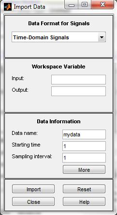
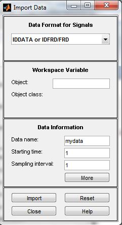
18 1.IMPORT DATA Identification

19 Identification 2.PREPROCESS DATA NEW (DETRENDED) DATA

20 3.ESTIMATE MODEL SELECT MODEL STRUCTURE Identification

21 Identification 3.1. MODEL STRUCTURES ARX(na,nb,k): A(z)y(t) = B(z)u(t) + e(t), where A(z)=1+ a_1 z^ a_na z^-na B(z)=b_1 z^-k b_nb z^-(k+nb) y(t)=-a_1 y(t-1)-...-a_na y(t-na) + b_1 u(t-k)+...+b_nb u(t-n_b-k)+e(t) ARMAX(na,nb,k): A(z)y(t) = B(z)u(t) + C(z)e(t), where A(z)=1+ a_1 z^ a_na z^-na B(z)=b_1 z^-k b_nb z^-(k+nb) C(z)=1+ c_1 z^ c_nc z^-nc y(t)=-a_1 y(t-1)-...-a_na y(t-na) + b_1 u(t-k)+...+b_nb u(t-n_b-k) +e(t)+c_1 e(t-1) c_nc e(t-nc)

22 Identification 3.1. MODEL STRUCTURES OE(nb,nf,k): y(t) = B(z)/F(z)u(t) + e(t), where B(z)=b_1 z^-k b_nb z^-(k+nb) F(z)=1+ f_1 z^ f_nf z^-nf y(t)=-f_1 y(t-1)-...-f_na y(t-nf) + b_1 u(t-k)+...+b_nb u(t-n_b-k) +e(t)+f_1 e(t-1) f_nf e(t-nf) BOX-JENKINS(nb,nc,nd,nf,k): y(t) = B(z)/F(z)u(t) + C(z)/D(z)e(t) STATE-SPACE (n: order) [PEM or subspace identification] x(t+1)=ax(t)+bu(t)+ke(t) y(t)=cx(t)+du(t)+e(t)

23 Identification 3.2. EXTERNAL REPRESENTATION MODEL STRUCTURES BOX-JENKINS WHY ARE THESE CLASSES OF INTEREST? OUTPUT ERROR (OE) ARX ARMAX

24 Identification ARX(na,nb,k): y(t)=-a_1 y(t-1)-...-a_na y(t-na) + b_1 u(t-k)+...+b_nb u(t-n_b-k)+e(t) OPTIMAL PREDICTOR: yp(t-1)=-a_1 y(t-1)-...-a_na y(t-na) + b_1 u(t-k)+...+b_nb u(t-n_b-k) least square method (COMPUTATIONALLY LIGHTWEIGHT). IF THE SYSTEM DOES NOT BELONG TO THIS MODEL STRUCTURE: BAD RESULTS ( WRONG POLES AND ZEROS)! OE(nb,nf,k): y(t) = B(z)/F(z)u(t) + e(t) OPTIMAL PREDICTOR: yp(t) = B(z)/F(z)u(t) The OPTIMAL PREDICTOR is the SIMULATOR (i.e., it does not need data). The simulation with OE is said Simulation Error Minimization. Computationally intensive It is able to well capture the dominant dynamics (poles and zeros) even if the model structure is not correct!

25 Identification 3.ESTIMATE MODEL IDENTIFICATION OF THE (CONTINUOUS-TIME) TRANSFER FUNCTION

26 Identification 3.ESTIMATE MODEL IDENTIFICATION OF MODELS: -NONLINEAR ARX - HAMMERSTEIN WIENER

27 4.Compare and validate models Identification

28 Identification For further details, see

29 Identification Other related Matlab functions (2 Identification toolbox) Parametric model estimation ar - AR-models of signals using various approaches. armax - Prediction error estimate of an ARMAX model. arx - LS-estimate of ARX-models. bj - Prediction error estimate of a Box-Jenkins model. ivar - IV-estimates for the AR-part of a scalar time series (with instrumental variable method). iv4 - Approximately optimal IV-estimates for ARX-models. n4sid - State-space model estimation using a sub-space method. nlarx - Prediction error estimate of a nonlinear ARX model. nlhw - Prediction error estimate of a Hammerstein-Wiener model. oe - Prediction error estimate of an output-error model. pem - Prediction error estimate of a general model.

30 Identification Model structure selection aic - Compute Akaike's information criterion. fpe - Compute final prediction error criterion. arxstruc - Loss functions for families of ARX-models. selstruc - Select model structures according to various criteria. idss/setstruc - Set the structure matrices for idss objects. struc - Generate typical structure matrices for ARXSTRUC. For more details please see: >> help ident

31 Exercizes Linear systems 1. Consider the discrete-time linear system, characterized by the following transfer function W z = 1+z z Plot the step response of the system. What are its features, in the light of the properties (stability, gain, etc.) of the systems? 1.2 Plot the response of the system to two different sinusoidal inputs, i.e., u(t)=sin(0.1t) and u(t)=sin(t). Analyze the properties of the two output signals in the light of the frequency response theorem.

32 Exercizes White noise 1. Define a 1000-samples realization of a Gaussian white noise with zero mean and unity variance λ 2 = 1. Verify that 68% of samples has absolute value smaller than λ and that 95% has absolute value smaller than 2λ. 2. Repeat the previous exercize in case λ 2 = Define a 1000-samples realization of a Gaussian white noise with mean μ = 10 and variance λ 2 = 4. Compare the obtained realization with that obtained at Exercize 2. Estimate the covariance function from the available data and verify that it corresponds with that expected in case of white noise.

33 Exercizes Identification of time series Consider the MA(1) stochastic process y(t), generated from the dynamic system y t = e t + 0.5e(t 1) with input e(t), i.e., white Gaussian noise with mean μ = 0 and variance λ 2 = 1. Define a realization of y(t) consisting of N=1000 samples. 1. Assume that the data generation system is unknown and the model class, selected for identification purposes, consists of a AR(1) process, i.e., y t = θy t 1 + ξ(t) where ξ(t) is a zero mean white noise process. 1.1 Compute, using the recursive least square method, the optimal estimate θ N of θ.

34 Exercizes 1.2 Define the evolution of the prediction error ε(t) = y t y(t t 1). Estimate its mean and variance Assuming that the data generation system is known, compute analytically the value of θ that minimizes the cost function J θ J θ. = E[ε(t) 2 ], and the corresponding value of

35 Exercizes Model Identification Consider the ARMAX system y(t)=0.1 y(t-1)+2u(t-1)-0.8 u(t-2)+e(t)+0.3e(t-1) Where e(t) is a white noise with zero mean and unitary variance. 1. Generate a 1000-samples realization of the output signal y(t), when the input u(t) is a persistently exciting signal (e.g., a white noise), and where y(0)=0;. 2. Identify, using the identification toolbox: 1. an ARX(1,1,1) model 2. an ARX(1,2,1) model 3. an ARMAX(1,2,2,1) model 4. an ARMAX(1,1,2,1) model 5. an OE(2,1,1) model 3. Compare and analyze the results (possibly add validation data to validate the results).

36 Exercizes Stationary stochastic processes 1. Consider the stochastic process y(t), generated from the dynamic system with a white noise e(t) as input. W z = 1+z z Assume that e(t) is a white Gaussian noise with mean μ and variance λ 2. Setting μ = 0 and λ 2 = 1, generate different realizations of both e(t) and y(t). Estimate, from the available data, mean and variance of the processes e(t) and y(t). 1.2 Show the results to the questions below in case μ = 10 and λ 2 = 1. What is the relationship between the mean of y(t) and the gain of the dynamic system W(z)?

37 Exercizes 2. Consider the stochastic process y(t), generated from the dynamic system with a white noise e(t) as input. W z = 1 z z Assume that e(t) is a white Gaussian noise with mean μ and variance λ 2. Setting μ = 0 and λ 2 = 1, generate different realizations of both e(t) and y(t). Estimate, from the available data, mean and variance of the processes e(t) and y(t). 2.2 Show the results to the questions below in case μ = 10 and λ 2 = Plot the spectra of the processes y(t) and y(t), i.e., Φ y ω = W(e jω ) 2 and Φ y ω = W(e jω ) 2. Is it possible to establish a relationship between the realizations of y(t) and y(t), are their respective spectra Φ y ω and Φ y ω?

38 Exercizes Predictors 1. Consider the stochastic process y(t), generated from the dynamic system W z = z z 1 with input e(t), i.e., white Gaussian noise with mean μ = 0 and variance λ 2 = Define the optimal 1-step predictor of y(t). 1.2 Define a realization of y(t) and the relative 1-step prediction y(t t 1). Compare the signals y(t) and y(t t 1), by drawing them in the same plot. 1.3 Define the signal ε(t) = y t y(t t 1) and plot it. Estimate mean and variance of ε(t). Compute analytically the theoretical values of the latter quantities and compare them with those obtaned from data.

39 Exercizes 1.4 Define now the trivial non optimal predictor y T t t 1 = E y t = 0. Estimate mean and variance of the estimation error in this case. 1.5 Compare the performances of the predictors defined above. 1.6 Define the optimal 2-step predictor y(t t 2) of y(t). 1.7 Define a realization of y(t) and the relative 1-step and 2-step predictions y(t t 1) and y(t t 2), respectively. Compare the signals y(t) and y(t t 1), and y(t t 2), by drawing them in the same plot. 1.8 Define the signal ε 2 (t) = y t y(t t 2) and plot it. Estimate mean and variance of ε 2 (t). Compute analytically the theoretical values of the latter quantities and compare them with those obtaned from data.