Matlab software tools for model identification and data analysis 10/11/2017 Prof. Marcello Farina

Transcription

1 Matlab software tools for model identification and data analysis 10/11/2017 Prof. Marcello Farina Model Identification and Data Analysis (Academic year ) Prof. Sergio Bittanti

2 Outline Data generation and analysis Definition and generation of time series and dynamic systems Analysis of systems Analysis of time series (sampled covariance and spectral analysis) Optimal predictors Identification Parameter identification Structure selection Model validation Exercizes

3 Time series and systems White noise >> N=100; % number of samples >> lambda=1; % standard deviation >> mu=1; % expected value I method >> u=mu+lambda*randn(n,1); II method >> u=wgn(m,n,p); % zero-mean signal M: number of signals P: signal power (dbw) (10log10(lambda^2)) Sum of a WGN and a generic signal >> u=awgn(x,snr,sigpower); X: original signal SRN: signal-to-noise ratio (db) SIGPOWER: power of signal X (dbw) (10log10( (0))) - if SIGPOWER= measured, AWGN estimates the power of signal X.

4 Time series and systems Definition of dynamic linear discrete-time systems: external representation (transfer function LTI format) >> system = tf(num,den,ts) num: numerator den: denominator Ts: sampling time (-1 default) >> system=tf([1 1],[1-0.8],1) Transfer function: z z - 0.8

5 Time series and systems Step response of a LTI system >> T=[0:Ts:Tfinal]; >> [y,t]=step(system,tfinal); % step response >> step(system,tfinal) % plot Response of a LTI system to a general input signal >> T=[0:Ts:Tfinal]; >> u1=sin(0.1*t); % e.g., sinusoidal input >> u2=1+randn(t,1); % e.g., white gaussian noise >> [y,t]=lsim(system,u1+u2,t);

6 Time series and systems The SYSTEM IDENTIFICATION TOOLBOX uses different formats for models (detto IDPOLY format) and signals (detto IDDATA format) Definition of IDDATA objects (i.e., inputs&outputs of a system in a single object): >> data=iddata(y,u,ts); u: input data y: output data Ts: sampling time

7 Time series and systems Definition of IDPOLY objects: >> model_idpoly = idpoly(a,b,c,d,f,noisevariance,ts) A,B,C,D,F are vectors (i.e., containing coefficients of the polynomials in incresing order of the exponent of z -1 ) Model_idpoly: A(q) y(t) = [B(q)/F(q)] u(t-nk) + [C(q)/D(q)] e(t) (If ARMAX: F=[], D=[]) The delay nk is defined in polynomial B(q). >> conversion from LTI format: Model_idpoly = idpoly(model_lti) model_lti is a LTI model (defined, e.g., using tf, zpk, ss) Response of an IDPOLY system to a generic input signal (vector u) >> y=sim(model_idpoly,u); -> It does not simulate the noise component, but just the deterministic one

8 Time series and systems Analysis of systems (both for LTI and IDPOLY formats): Zeros and poles: >> [Z,P,K]=zpkdata(model) Z = [-1] % positions of the zeros P = [0.8000] % positions of the poles K = 1 transfer constant Bode diagrams: >> [A,phi] = bode(model,w) W: values of the angular frequency w where to compute A(w) and phi(w) A: amplitude (A(w)) Phi: phase (phi(w))

9 Time series and systems Bode diagrams: >> [A,phi] = bode(model,[0.1 1]) A(:,:,1) = A(:,:,2) = phi(:,:,1) = phi(:,:,2) = >> bode(model) >> % draws the Bode plots (amplitude db- and phase)

10 Time series and systems Analysis of time series - m=mean(x) % Average or mean value. Y=detrend(X, constant ) % Remove constant trend from data sets. Y=detrend(X, linear ) % Remove linear trend from data sets. Covariance function ϒ( ) >> gamma=covf(y,10) % tau=0,1,,10-1 >> plot([0:9],gamma) Spectrum (!) periodogram method >> periodogram(y); % plots the periodogram >> [Pxx,w]=periodogram(y); >> plot(w/pi,10*log10(pxx)) Other methods are also available (e.g., fast fourier transform, see «help spectrum») Warning: covf computed the correlation function! TO OBTAIN THE COVARIANCE FUNCTION THE SIGNAL MUST HAVE ZERO MEAN Warning: no regularization technique is applied: the estimator is not consistent!

11 Predictors

12 Predictors

13 Predictors >> [ypred, x0_est, pred_model] = predict(model, data, k) INPUTS: model idpoly object data iddata object k prediction steps (integer number) OUTPUT ypred y_hat(t+1/t), predicted output, iddata object x0_est estimate of the initial condition (for state_space model) pred_model prediction model (discrete-time state-space model): >> pred_model_tf = tf(pred_model) % to obtain the transfer functions From input "y1" to output "y1": From input "u1" to output "y1 : It includes the prediction delay It includes the control delay

14 - EXAMPLE 1 (ARMAX model): Predictors >> Model_idpoly=idpoly([1 0.3],[ ],[1 0.5],[],[],1,1) Discrete-time IDPOLY model: A(q)y(t) = B(q)u(t) + C(q)e(t) A(q) = q^-1 B(q) = q^-1 C(q) = q^-1 tau = 1 % control delay >> [yd,xoe,modpred]=predict(model_idpoly,data,1); >> tf(modpred) From input "y1" to output "y1": 0.2 z^ z^-1 From input "u1" to output "y1": z^ z^ z^-1

15 Predictors - EXAMPLE 2 (OE model): >> Model_idpoly=idpoly([1 0.3],[ ],[1 0.3],[],[],1,1) Discrete-time IDPOLY model: A(q)y(t) = B(q)u(t) + C(q)e(t) A(q) = q^-1 B(q) = q^-1 C(q) = q^-1 tau = 1 % control delay >> [yd,xoe,modpred]=predict(model_idpoly,data,1); >> tf(modpred) From input "y1" to output "y1": 0 From input "u1" to output "y1": z^ z^ z^-1

16 Predictors - EXAMPLE 3 (ARX model): >> Model_idpoly=idpoly([1 0.3],[ ],[1],[],[],1,1) Discrete-time IDPOLY model: A(q)y(t) = B(q)u(t) + C(q)e(t) A(q) = q^-1 B(q) = q^-1 C(q) = 1 tau = 1 % control delay >> [yd,xoe,modpred]=predict(model_idpoly,data,1); >> tf(modpred) From input "y1" to output "y1": -0.3 z^-1 From input "u1" to output "y1": z^ z^-2

17 Prediction error Predictors >> Epsilon = pe(model_idpoly,data) % k-steps prediction error ARDERSON TEST FOR THE PREDICTION ERROR (99% confidence reguion) >> e=resid(model_idpoly,data) inputs model: IDPOLY format data: IDDATA format (input-output data) outputs e: IDDATA ([prediction error,input]) If the outputs are not specified, a plot is shown: - Empirical correlation function (empirical - sampled) of the prediction error - 99% confidence region -> if more than 99% of the samples of the normalized correlation function lie in the confidence region: positive results of the whiteness Test!

18 Example: Predictors >> A_idpoly=[1 0.3]; >> B_idpoly=[0 1 1/5]; %tau=1 >> C_idpoly=[1 1/2]; >> Model_idpoly = idpoly(a_idpoly,b_idpoly,c_idpoly,[],[],sigma,1); >>[yd,xoe,modpred]=predict(model_idpoly,data,1); >> resid(model_idpoly,data) >> data2=iddata(randn(n,2),1); >> resid(model_idpoly,data2) Correlation function of residuals. Output y Correlation function of residuals. Output y1 lag Cross corr. function between input u1 and residuals from output y

19 Identification >> systemidentification % start the MATLAB identification toolbox GUI

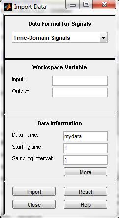
20 1.IMPORT DATA Identification

21 Identification 2.PREPROCESS DATA NEW (DETRENDED) DATA

22 3.ESTIMATE MODEL SELECT MODEL STRUCTURE Identification

23 Identification 3.1. MODEL STRUCTURES ARX(na,nb,k): A(z)y(t) = B(z)u(t) + e(t), where A(z)=1+ a_1 z^ a_na z^-na B(z)=b_1 z^-k b_nb z^-(k+nb-1) y(t)=-a_1 y(t-1)-...-a_na y(t-na) + b_1 u(t-k)+...+b_nb u(t-n_b-k+1)+e(t) ARMAX(na,nb,nc,k): A(z)y(t) = B(z)u(t) + C(z)e(t), where A(z)=1+ a_1 z^ a_na z^-na B(z)=b_1 z^-k b_nb z^-(k+nb-1) C(z)=1+ c_1 z^ c_nc z^-nc y(t)=-a_1 y(t-1)-...-a_na y(t-na) + b_1 u(t-k)+...+b_nb u(t-n_b-k+1) +e(t)+c_1 e(t-1) c_nc e(t-nc)

24 Identification 3.1. MODEL STRUCTURES OE(nb,nf,k): y(t) = B(z)/F(z)u(t) + e(t), where B(z)=b_1 z^-k b_nb z^-(k+nb-1) F(z)=1+ f_1 z^ f_nf z^-nf y(t)=-f_1 y(t-1)-...-f_na y(t-nf) + b_1 u(t-k)+...+b_nb u(t-n_b-k+1) +e(t)+f_1 e(t-1) f_nf e(t-nf) BOX-JENKINS(nb,nc,nd,nf,k): y(t) = B(z)/F(z)u(t) + C(z)/D(z)e(t) STATE-SPACE (n: order) [PEM or subspace identification] x(t+1)=ax(t)+bu(t)+ke(t) y(t)=cx(t)+du(t)+e(t)

25 Identification 3.2. EXTERNAL REPRESENTATION MODEL STRUCTURES BOX-JENKINS WHY ARE THESE CLASSES OF INTEREST? OUTPUT ERROR (OE) ARX ARMAX

26 Identification ARX(na,nb,k): y(t)=-a_1 y(t-1)-...-a_na y(t-na) + b_1 u(t-k)+...+b_nb u(t-n_b-k+1)+e(t) OPTIMAL 1-step PREDICTOR: yp(t-1)=-a_1 y(t-1)-...-a_na y(t-na) + b_1 u(t-k)+...+b_nb u(t-n_b-k+1) least square method (COMPUTATIONALLY LIGHTWEIGHT). IF THE SYSTEM DOES NOT BELONG TO THIS MODEL STRUCTURE: BAD RESULTS ( WRONG POLES AND ZEROS)! In our example, we estimate from data an ARX model [1 2 1] (with N=10000 data): Discrete-time IDPOLY model: A(q)y(t) = B(q)u(t) + e(t) A(q) = ( ) q^-1 B(q) = q^ ( ) q^-2 Estimated using ARX from data set edat Loss function and FPE Sampling interval: 1

27 OE(nb,nf,k): y(t) = B(z)/F(z)u(t) + e(t) OPTIMAL PREDICTOR: yp(t) = B(z)/F(z)u(t) Identification The OPTIMAL PREDICTOR is the SIMULATOR (i.e., it does not need data). The simulation with OE is also said Simulation Error Minimization. Computationally intensive It is able to well capture the dominant dynamics (poles and zeros) even if the model structure is not correct! In our example, we estimate from data a OE model [2 1 1] (with N=10000 data): Discrete-time IDPOLY model: y(t) = [B(q)/F(q)]u(t) + e(t) B(q) = q^ ( ) q^-2 F(q) = ( ) q^-1 Estimated using PEM using SearchMethod = Auto from data set z Loss function and FPE Sampling interval: 1

28 Identification In our example, we estimate from data a ARMAX model [ ] (with N=10000 data) i.e., the right model structure: Discrete-time IDPOLY model: A(q)y(t) = B(q)u(t) + C(q)e(t) A(q) = ( ) q^-1 B(q) = q^ ( ) q^-2 C(q) = ( ) q^-1 Estimated using PEM using SearchMethod = Auto from data set z Loss function and FPE Sampling interval: 1 Both with OE model class and with ARMAX model class (the structure of the data generator) we are able to correctly estimate the transfer function u->y

29 Identification 3.ESTIMATE MODEL IDENTIFICATION OF THE (CONTINUOUS-TIME) TRANSFER FUNCTION

30 Identification 3.ESTIMATE MODEL IDENTIFICATION OF MODELS: -NONLINEAR ARX - HAMMERSTEIN WIENER

31 4.Compare and validate models Identification

32 Identification For further details, see

33 Identification Other related Matlab functions (2 Identification toolbox) Parametric model estimation ar - AR-models of signals using various approaches. armax - Prediction error estimate of an ARMAX model. arx - LS-estimate of ARX-models. bj - Prediction error estimate of a Box-Jenkins model. ivar - IV-estimates for the AR-part of a scalar time series (with instrumental variable method). iv4 - Approximately optimal IV-estimates for ARX-models. n4sid - State-space model estimation using a sub-space method. nlarx - Prediction error estimate of a nonlinear ARX model. nlhw - Prediction error estimate of a Hammerstein-Wiener model. oe - Prediction error estimate of an output-error model. pem - Prediction error estimate of a general model.

34 Identification Model structure selection aic - Compute Akaike's information criterion. fpe - Compute final prediction error criterion. arxstruc - Loss functions for families of ARX-models. selstruc - Select model structures according to various criteria. idss/setstruc - Set the structure matrices for idss objects. struc - Generate typical structure matrices for ARXSTRUC. For more details please see: >> help ident

35 Exercizes

36 Exercizes

37 Exercizes

38 Exercizes

39 Exercizes Model Identification Consider the ARMAX system y(t)=0.1 y(t-1)+2u(t-1)-0.8 u(t-2)+e(t)+0.3e(t-1) Where e(t) is a white noise with zero mean and unitary variance. 1. Generate a 1000-samples realization of the output signal y(t), when the input u(t) is a persistently exciting signal (e.g., a white noise), and where y(0)=0;. 2. Identify, using the identification toolbox: 1. an ARX(1,1,1) model 2. an ARX(1,2,1) model 3. an ARMAX(1,2,2,1) model 4. an ARMAX(1,1,2,1) model 5. an OE(2,1,1) model 3. Compare and analyze the results (possibly add validation data to validate the results).

40 Exercizes

41 Exercizes

42 Exercizes

43 Exercizes