2.161 Signal Processing: Continuous and Discrete

Transcription

1 MIT OpenCourseWare Signal Processing: Continuous and Discrete Fall 2008 For information about citing these materials or our Terms of Use, visit:

2 MASSACHUSETTS INSTITUTE OF TECHNOLOGY DEPARTMENT OF MECHANICAL ENGINEERING 2.6 Signal Processing - Continuous and Discrete Fall Term 2008 Solution of Problem Set 9 Assigned: November 20, 2008 Due: December 4, 2008 Problem : + + = xp(x)dx = x(λe λx )dx = e λx + ( x ) = λ λ µ x σ x = µ x 2 µ x = x 2 p(x)dx µ x = x2 (λe λx )dx 0 2 σ 2 = e λx 2 ( x + 2 ( x )) + x 0 = = λ λ λ 2 λ 2 λ 2 λ 2 σ x = λ λ 2 Problem 2: Φ ff ( jω) H ( j ω ) Φ gg ( j ω) - ω c ω c Input f is a white noise with flat spectrum and hence we assume that Φ ff (jω) =. The output can be computed from: Φ gg (jω) = H(jω) 2 Φ ff (jω) = H(jω) 2. = H(jω) 2 + ω c Φ gg (τ) = F (Φ gg (jω)) = H(jω) 2 e jwτ dω =.e jωτ ω c dω = sinc(ω c τ) = sin(ω cτ) 2π 2π π πτ ω c

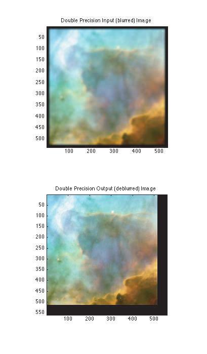
3 Problem 3:. M, E I J H J E C. E J A H / M. M 0 M L A H I A. E J A H 4 M. M 0 M 0 M 0 M 0 M. M The inverse filter for this high-precision problem can be implemented as the exact inverse of the input filter. We will revisit this problem in the 2nd quiz where additive noise of quantization imposes some modification to the inverse filter. Here is the code that we used. - Note that h kernel needs to be zero padded such that that image and h DFT have the same size. This ensures that their corresponding DFT matrix elements, correspond to the same (u, v) value and we can multiply them element-wise. - Note the color scaling at the end. All the color channels are scaled with the same scale, such that relative RGB pattern is not altered. clear all,close all,clc %% Read in the image load( blurredimage2.mat, blurred ) figure,subplot(2,,),image(blurred), axis image title( Double Precision Input (blurred) Image ) %% Determine the size of the image supplied pad = 24; imsize = size(blurred); xsize = imsize() + pad;ysize = imsize(2) + pad; % Take fft of image fftblur = fft2(blurred,xsize,ysize); % %% Design the inverse filter % Use a gaussian kernel from the image processing toolbox hsize=25;sigma = 3; h = fspecial( gaussian, hsize, sigma); ffth = fft2(h,xsize,ysize); % Create the inverse filter - this is just the simple form: fftinvh =./ffth; % figure % mesh(fftshift(abs(fftinvh))) % title( Inverse Filter Magnitude ) % %% Filter the image fftdeblur = zeros(xsize,ysize,3); for i=:3 fftdeblur(:,:,i) = fftinvh.*fftblur(:,:,i); end %% Inverse fft and Color Intensity Scaling deblurred = abs(ifft2(fftdeblur)); % Normalize the pixel intensity for the whole image % to set all values in the range 0 -- (already all are positive) maxpix = max(max(max(max(deblurred))),); deblurred = deblurred/maxpix; % Show the image subplot(2,,2),image(deblurred), axis image title( Double Precision Output (deblurred) Image ) 2

4 Double Precision Input (blurred) Image Double Precision Output (deblurred) Image

5 4

6 Problem 4: (This is from the take-home Quiz 2 from last year.) (a) The autocorrelation of the contaminated signal is φ gg (τ) = E {g(t)g(t + τ)} = E {(f(t) + αf(t Δ))(f(t + τ) + αf(t + τ Δ))} { } = E {(f(t)f(t + τ)} + E α 2 f(t Δ)f(t + τ Δ) +E {αf(t)f(t + τ Δ)} + E {αf(t + τ)f(t Δ)} and recognizing that φ ff (τ) does not depend on the time origin, (b) With the MATLAB code φ gg (τ) = ( + α 2 )φ ff (τ) + αφ ff (τ Δ) + αφ ff (τ + Δ) [f,fs,nbits] = wavread( PS9Prob4.wav ); L = length(f); figure(), plot(-(l-):l-, xcorr(f,f)) the following plot was annotated using the cursor tip Autocorrelation of input data X: 0 Y: X: 200 Y: 5.59 X: 200 Y: 5.59 phi shift 4 x 0 5

7 We assume that φ ff (0) >> φ ff (2τ), φ ff (τ) and then from (a) peaks on the graph correspond to: ( + α 2 )φ ff (0) αφ ff (0) 5.59 or α α + = 0 so that α Actually α = 0.3 and we will use α = 0.3 value. Similarly, from the autocorrelation function m = 200. (c) Recognize that Eq. (2) is a filter with H(z) = +αz Δ. Then the inverse filter H (z) = /H(z) to remove the echo is H (z) = + αz Δ which is an IIR filter with a difference equation f n = αf n m + g n. (d) Below is the complete MATLAB code to implement the filter and filter the data: [f,fs,nbits] = wavread( PS9Prob4.wav ); L = length(f); figure(), plot(-(l-):l-, xcorr(f,f)) title( Autocorrelation of input data ) xlabel( shift ) ylabel( phi ) % Look at the autocorrelation function wavplay(f,fs) % Determine that the delay is 200 and alpha=0.3 delay = 200; alpha = 0.3; % Recursive filter: % Set up the denominator: a = zeros(,20); a() = ; a(20) = alpha; y = filter(, a, f); figure(2), plot(-(l-):l-, xcorr(y,y)) title( Autocorrelation of processed data (IIR filter) ) xlabel( shift ) ylabel( phi ) % wavplay(f,fs) which produced the following output autocorrelation plot 6

8 60 Autocorrelation of processed data (IIR filter) phi shift 4 x 0 Note that the echo components have been eliminated. 7