Chapter 3. Nuclear Reactions in Stars. preliminaries: relating rates to cross sections; thermal distrubutions; thermally averaged

Transcription

1 Chapter 3 Nuclear Reactions in Stars This chapter is divided into three parts: preliminaries: relating rates to cross sections; thermal distrubutions; thermally averaged rates; and the S-factor application to the pp chain He burning 3.1 Rates and cross sections We want to consider the reaction 1(p 1 )+2(p 2 ) 1 (p 1 )+2 (p 2 ) where the four-momentum of particle 1 is given by p 1, etc. The rate (events/unit time in some volume V) is dn dt = d x ρ 1 (p 1, x) ρ 2 (p 2, x) v 1 v 2 σ 12 (p 1,p 2 ) where ρ 1 (p 1, x) is the number density of particles of type 1 with four-momentum p 1 (that is, the number of particles per unit volume). The relative velocity is defined v 1 v 2 = (p 1 p 2 ) 2 m 2 1m 2 2 E 1 E 2 where the dot product the the four vector is defined p 1 p 2 = E 1 E 2 p 1 p 2 To convince yourself that this is a reasonable definition: 1) Evaluate this in the rest frame of particle 2, which mean p 2 =(m 2, p 2 = 0). The answer is p 1 /E 1 = v 1. 2) Evaluate this for 1 and 2 being nonrelativistic, so that p 1 =(m 1 + p 1 2 2m 1, p 1 ). One finds the result 1

2 m 1 m 2 v 1 v 2 E 1 E 2 v 1 v 2 Suppose the densities above are constant over the volume of interest (some region within a star). Then the integral over x is simple, yielding r =events/unit time/unit volume = 1 V dn dt = ρ 1ρ 2 1+δ 12 v 1 v 2 σ 12 Note the factor of 1 + δ 12. The rate should be proportional to the number of pairs of interacting particles in the volume. If the particles are distinct, that is just ij ρ 1 ρ 2 But if the particles are identical, the sume over distinct pairs is 1 2 ij 1 2 ρ 1ρ Decay rates Another process of interest in stars in the decay of particle 1 to possible final states, which we might number 2,3,4, etc. In this case 2 might stand for a final nucleus, an electron, andanantineutrino,inthecaseofβ decay. The rate can be written r =no. decays/unit time/unit volume = ρ 1 (ω 12 + ω 13 + ω ) where ω 12 is the decay rate for the channel 1 2 and is given in units of 1/sec. The mean lifetime is defined Note that the halflife is defined by As the total decay rate is τ 12 = t = 0 e ω 12t tdt = 1 ω = 1/2 e ω 12τ12 τ 1/2 12 = ln 2 =ln2τ 12 ω 12 2

3 ω total = ω 12 + ω it follows 1 τ total = 1 τ τ Thermal distributions The particles in our stellar plasma have a distribution of momenta characterized by their temperature. Thus to get total rates we need to integrate the expressions above over those distributions. We consider three distributions: a) Maxwell Boltzmann distribution b) Fermi-Dirac distribution n s = g s e (ɛs µ)/kt c) Bose-Einstein n s = g s e (ɛs µ)/kt +1 n s = g s e (ɛs µ)/kt 1 The particle energy ɛ s above is m + p 2 + m 2. (Often the rest mass term m is omitted because it can be absorbed into the chemical potential. But one should include it explicitly when nuclear binding energies have to be considered: the Saha equation discussion will illustrate this.) The parameter µ, the chemical potential, is determined for fixed T and particle density: an example will be done below. 3

4 The Fermi-Dirac distribution describes identical fermions. The usual custom is to write µ = ɛ F.AskT 0, g s e (ɛs ɛ F )/kt +1 0ifɛ s ɛ F g s if ɛ s ɛ F Thus ɛ F is often called the Fermi level, as it divides the low-energy completely occupied levels from the higher energy completely unoccupied levels. Of course, at finite temperatures, this demarcation is not sharp. We can integrate over some finite, uniform volume V to count the total number of contained fermions N o = V h 3 d g s k e (ɛ ɛ F )/kt +1 [ ] In this expression (ɛ, k) is the particle four-momentum and g s represents the REMAINING degeneracy of the quantum level of energy ɛ, e.g., perhaps the spin and isospin degeneracy. The degeneracy due to momentum d k =4πk 2 dk where ɛ = k2 2m is included explicitly in the integral. We can rewrite the above integral as an integral over energy N o = V h 4π g s 2m 3 ɛdɛ 3 0 e (ɛ ɛ F )/kt +1 Now at kt = 0 the exponential goes to zero for ɛ ɛ F and infinity otherwise. Therefore N o = V h 4π g ɛf s 2m 3 ɛdɛ 3 0 which then defines the Fermi energy ɛ F in terms of the number density N o /V ( ) 1/3 ( ) ɛ F (kt =0)= h2 1 2/3 3No m 2 g s 2 8πV 4

5 Note for electrons, with two spin states, the second factor on the RHS would be 1/2 ( g s = 1/2). It should be clear that for general kt, one has to solve the full equation [*] to relate ɛ F to kt, N o. And it turns out the ɛ F is a slowly varying function of kt. A picture of N(ɛ), the number of particles of energy ɛ, is sketched on the following page. The region around the Fermi surface gradually softens as kt is increased, in accordance with the naive expectation that particles with kt of the Fermi surface ought to be occasionally excited above the Fermi surface. The Maxwell-Boltzmann distribution describes the behavior of identical, distinguishable particles and can be thought of as the classical limit of Fermi-Dirac statistics, where quantum effects associated with exchange are unimportant. The common situation we will encounter is when the density is low (so that ɛ F goes to 0) and the particles are nonrelativistic. Then ɛ s /kt is a large number, and the Fermi-Dirac distribution goes over to the Maxwell- Boltzmann distribution. We used this result in the big bang discussion, where these two conditions are met. Some typical uses of the Maxwell-Boltzmann distribution in astrophysics: Describing the occupation of levels in well-isolated atoms. This is appropriate when quantum effects due to electrons in the plasma and due to other atoms are unimportant. Describing molecular excitations, such as rotations. As an example, consider a two-level atom, that is, one with a ground state (which we will take to be 1s 1/2 ) and an excited state 1p 3/2. The MB weights are, respectively, 2e ɛgs/kt and 4e ɛex/kt Thus the population of the excited state is 5

6

7

8 2e (ɛex ɛgs)/kt 1+2e (ɛex ɛgs)/kt The result we will use frequently is the Maxwell-Boltzmann velocity distribution law, which comes immediately from [*] N 1 ( v 1 )d v 1 = N 1 ( m 1 2πkT )3/2 e m 1v2 1 /kt d v 1 We have already used the Bose-Einstein distribution, which describes the distribution of identical bosons, when we related T to ρ γ in Chapter 1. It has additional astrophysics applications in matters such as pion and kaon condensation in dense nuclear matter, etc. 3.4 Saha equation Let s consider a problem addressed before n + p d + γ During the period of interest to us in BBN these nuclear species are nonrelativistic and nondegenerate - a dilute gas that can be accurately described by Maxwell-Boltzmann statistics. The nuclear species n, p, andd are in thermal equilibrium. Previously we studied the detailed balance - primarily to illustrates the role of the high-energy tail of the photon distribution. Here we do things more correctly, using that we know statistical equilibrium holds. We have three nuclear species and a partition function for each one, e.g., Z p n e (µp E(n))/kT We can write the probability function, noting each species is a set of indistinguishable particles, S(N p,n n,n d )= ZNp p N p! Z Nn n N n! Z N d d N d! 6

9 The Zs aregivenby Z p = V h g 3 p e [µp mp p2 /(2m p)]/(kt) d 3 p The integral can be done, yielding Similarly Z p = g pv h 3 e[µp mp]/(kt) (2πm p kt) 3/2 Z n = g nv h 3 e[µn mn]/(kt) (2πm p kt) 3/2 Z d = g dv h 3 e[µ d m d ]/(kt) (2πm d kt) 3/2 Now we want to find the most probable state, which maximizes S(N p,n n,n d ). We note that ln(s) will have the same maximum at S. And ln(n!) nln(n) n for large n, by Stirling s formula. So lns = N p lnz p + N n lnz n + N d lnz d N p lnn p + N p N n lnn n + N n N d lnn d + N d Now let N T p and N T n be the total number of protons and neutrons, regardless of whether they are free or bound. These numbers are constant (integrated over all volume) and N d = N T p N p N d = N T n N n N n = N T n N T p + N p That is, we can take N p as our one variable with lns = N p lnz p +(N T n N T p + N p )lnz n +(N T p N p )lnz d N p lnn p + N p + N T n (N T n N T p + N p)ln(n T n N T p + N p) (N T p N p)ln(n T p N p) 7

10 Thus d(lns) d(n p ) lnz p + lnz n lnz d lnn p ln(n T n N T p + N p)+ln(n T p N p)=0 so that at maximum probability Z p Z n Z d = N pn n N d N d = N p N n h 3 V g d g n g p ( A d A p A n ) 3/2 (2πm N kt) 3/2 e [µ d µ n µ p m d +m n+m p]/(kt) Here we have taken m p A p m N, m n A n m N,andm d A d m N in the mass ratio, where A d =2,A p =1,andA n = 1 are the atomic numbers of the three species. Converting to number densities (divide by V) g d n d = h 3 n p n n ( A d ) 3/2 (2πm N kt) 3/2 e [µ d m d µ p+m p µ n+m n]/(kt) g p g n A n A p Now at equilibrium µ d µ p µ n = 0: the chemical potential is defined as the change in the system energy on adding a particle. Since n + p is in equilibrium with d, the change in energy on adding a neutron and a proton is the change in energy on adding a deuteron. Also the deuteron binding energy this is defined as a positive quantity is B d = m p + m n m d. Finally we define the mass fractions by X d = A dn d n N X F p = A pn p n N X F n = A dn d n N where the superscript F denotes these are the free p/n mass fractions and where n N = (N T p +N T n )/V is the total number density of nucleons, free or bound. Note X d+x F p +XF n =1. It follows 8

11 g d X d = Xp F XF n nh3 ( A d ) 5/2 (2πm N kt) 3/2 e B d/(kt) g p g n A p A n = X F p XF n η g d g p g n ( A d A p A n ) 5/2 T 3/ e 25.83/T 9 where we have used a result from Chapter 2 for the photon number density to rewrite this in terms of the baryon/photon ratio η. T 9 is the temperature in units of 10 9 degree Kelvin. (We have left the As andgs in to the end so that this formula can be used for any reaction.) Now g d =3 (the deuteron ground state has J=1), g p =2, g n =2 so X d = X F p X F n ηt 3/ e 25.83/T 9 So let s solve this for the temperature of deuterium formation. As before, that is defined when half the neutrons are bound. In terms of mass fractions this means the free neutron mass fraction 2X F n = X d.wealsoknown/p =1/7 at freezeout, which means X d /(X F n + X F p )= 1/7. And X F n + XF p + X d = 1. All of this yields X F n = 1 16 X F p = X d = 1 8 So that = ηt 3/2 9 e 25.83/T 9 which relates η and T d. We find for η =10 9 that T d =0.785 and for η =10 10 T d =0.733, in units of 10 9 Kelvin. Thus this is a much nicer way of deriving the η-t d relationship discussed in Chapter Thermally averaged rates We now discuss reactions of nonrelativistic charged nuclei in a stellar plasma, where the nuclei have a distribution of velocities. The rate formula discussed earlier for can be generalized to take care of the velocity distribution r = N 1N 2 1+δ 12 vσ 12 (v) N 1N 2 1+δ 12 vσ 12 (v) 9

12 where represents a thermal average. Note that we have written the cross section as a function of the relative velocity v: this is ok as the total cross section is invariant under Galilean transformations (as is the rate), so it must have this form. Now we use our Maxwell-Boltzmann velocity distribution N 1 N 1 ( v 1 )d v 1 = N 1 ( m 1 2πkT )3/2 e m 1v2 1 /2kT d v 1 to define this thermal average vσ 12 (v) = d v 1 d v 2 ( m 1 2πkT )3/2 ( m 2 2πkT )3/2 e (m 1v2 1 +m 2 v2 2 )/2kT σ 12 (v)v We introduce the center-of-mass and relative velocities v cm = m 1 v 1 + m 2 v 2 m 1 + m 2 v rel = v = v 1 v 2 so that v 1 = v cm + m 2 v m 1 + m 2 v 2 = v cm m 1 v m 1 + m 2 With these definitions, e (m 1v 2 1 +m 2v 2 2 )/2kT = e ((m 1+m 2 )v 2 cm +µv2 )/2kT where µ = m 1m 2 m 1 +m 2 is the reduced mass. Now d v 1 d v 2 = d( v 1 v 2 )d( v 1 + v 2 )= 2 2 d vd( v 1 + v 2 ) 2 10

13 But v cm = 1 2 ( v 1 + v 2 )+ 1 2 (m 1 m 2 m 1 + m 2 ) v Therefore d v 1 d v 2 = d v d v cm If we make this transformation in our expression for r, the entire dependence on v cm is d v cm e (m 1+m 2 )vcm 2 /2kT 2πkT =( ) 3/2 m 1 + m 2 So we derive our desired result r = N 1N 2 ( 1+δ 12 µ 2πkT )3/2 d vσ 12 (v)ve µv2 /2kT important result: the relative velocity distribution is a Maxwellian based on the reduced mass This can be written r = N 1N 2 4π( 1+δ 12 µ 2πkT )3/2 0 v 3 dvσ 12 (v)e µv2 /2kT In the center of mass v cm =0 v 1 = m 2 m 1 v 2 so that v = v 1 v 2 = v 1 ( m 1 + m 2 m 2 ) Thus m 2 m 1 v 1 =( ) v v 2 = ( ) v m 1 + m 2 m 1 + m 2 11

14 leading to E = E cm = m 1 2 v2 1 + m 2 2 v2 2 = µ 2 v2 Therefore de = µvdv and 3.6 Nonresonant reactions r = N 1N δ 12 πµ ( 1 kt )3/2 EdEσ 12 (E)e E/kT 0 Nuclear reactions of various types can occur in stars. The first division is between charged reactions and neutron-induced reactions. The physics distinctions are the Coulomb barrier suppression of the former, and the need for a neutron source in the latter. The charged particle reactions can also be divided in several classes. First, it is helpful to develop a general physical picture of the process as the merging of 1 and 2 to form a compound nucleus, followed by the decay of that nucleus into The notion of the compound nucleus is important: a nucleus is formed that is clear unstable, as it was formed from 1+2 and therefore can decay at least into the 1+2 channel. Yet it is a long-lived state in the sense that it exists for a time much much longer than the transit time of a nucleon to cross the nucleus. Although the picture is not entirely accurate, it is nevertheless helpful to envision the following analogy. Imagine a shallow ashtray, the bottom of which has a fairly uniform covering of marbles. Now put a marble on the flat lip of the ashtray and give it a push, so that it rolls to the bottom of the ashtray with some kinetic energy. All collisions will be assumed elastic. Thus the system that one has created is unstable: there is enough energy for the system to eject the marble back to the lip of the ashtray and thus off to infinity. But once the marble collides with the other marbles in the bottom of the ashtray, the energy is shared among the marbles. It becomes extremely improbable for one marble to get all of the energy, enabling it to escape. This is thus the picture of a compound nucleus, an unstable state that nevertheless is long lived, as it can only fission by a very improbable circumstance where one nucleon (or group of nucleons) 12

15 acquires sufficient energy to escape. If one probes a nucleus above its particle breakup threshold - this would be the intermediate nucleus in the discussion above - one will observe resonances, states that are not eigenstates but instead are unstable and thus have some finite spread in energy. You may be familiar with some examples from quantum mechanics: the case often first studied is the shape resonances that occur when scattering particles off a well, such as a square well. Such states usually carry a large fraction of the scattering strength and can be thought of as quasistationary states. The charged particles break up into two classes, resonant (where the incident energy corresponds to a resonance) and nonresonant. The first applications we will make involve nonresonant reactions, so this is the example we will do in some detail. A picture of a nonresonant charged particle reaction is shown in the figure. It depicts barrier penetration: the incident energy is well below the Coulomb barrier, so the classical turning point is well outside the region of the strong potential where fusion can occur. But this energy is not coincident with any of the resonant quasistates. Suppose we were interested in the reaction 3 H + 4 He 7 Be 7 Be(g.s.)+γ where 7 Be is the intermediate nucleus formed in the fusion. To calculate the cross section, it will prove sufficient to ask the following question: given the nucleus 7 Be, what is the probability for it to decay into the channels 3 H + 4 He and 7 Be(g.s.)+γ? The former will be related by time reversal to the probability for forming the compound nucleus. For definiteness we ask for the rate for decaying into 3 H + 4 He. Thisis 13

16 r 0 ~ 1.44 A 1/3 fm V(r) Tunnelling through coulomb barrier for nuclear fusion Z 1 Z 2 E MeV 30 MeV Figure 1: Sketch of the potential as a function of distance r between two fusing nuclei. Nuclear attraction dominates for r < r 0, and repulsive Coulomb barrier dominates at r > r 0. Here A is the mass number of the nucleus. A particle of energy E lower than the Coulomb barrier must tunnel through the barrier for fusion to be accomplished. r

17 λ( 7 Be )= 1 τ =prob./sec for flux of 3 H/ 4 He through a sphere at very large r where r is the relative coordinate of the 3He and 4He. This can be written lim(r ) v r 2 sin θdθdφ Ψ(r, θ, φ) 2 = lim(r ) v χ l(r) 2 Y lm 2 r 2 sin θdθdφ = v χ l ( ) 2 r Note that χ l ( ) 2 is a constant for very large r. We can write this result as follows λ = vp l χ l (R N ) 2 P l = χ l( ) 2 χ l (R N ) 2 where χ l (R N ) 2 is a strong interaction quantity that depends on the wave function at the nuclear radius. The first term above is the penetration factor, the square of the ratio of the wave function at the nuclear surface to that an infinity. If the Coulomb barrier is high, this penetration factor will be very small because the tunneling probability is low. The simplest estimate of this would come from treating the wave function as a pure Coulomb wave function. The Coulomb radial equation is ( 1 d 2 l(l +1) + + αz 1X 2 2µ dr2 2µr 2 r E)χ l (r) =0 where r is the relative 3 H- 4 He coordinate. Defining E = p/2µ ρ = pr η = αz 1Z 2 v = αz 1Z 2 µ p = αz 1 Z 2 µ 2E the outgoing solution corresponds to the following combination of the standard Coulomb functions A(G l (ρ)+if l (ρ)) (as r ) A(e i(pr lπ/2 η ln 2p+σ l) Ae ipr 14

18 Thus we find the penetration factor P l = χ l( ) 2 χ l (R N ) 2 = 1 F l (pr N ) 2 + G l (pr N ) 2 And values for the penetration could be obtained by looking up numerical values. While the above is formally an exact solution in the region outside the nuclear potential, it is difficult to see the physics. But there is an approximate approach that does bring out the physics, illustrating both the basic penetration probability and the effects of higher partial waves and the finite nuclear radius. The method is described in Clayton and is based on the WKB approximation, in which the Schroedinger equation is solved via an expansion in powers of h. Thus this is a semiclassical approximation. The derivation takes a full lecture and thus is not appropriate here. So I will just quote the answer and refer those interested to Clayton. P WKB l Ec E e [ ] 2παZ 1 Z µR v 2 2l(l+1) N Ec 2µR 2 N Ec where E c = Z 1 Z 2 α/r N is the Coulomb potential at the nuclear surface and R N is the nuclear radius. This expression for the penetration factor consists of three terms The leading Gamow factor, which also comes from the l=0 Coulomb expression we derived earlier The effects of the angular momentum barrier, proportional to l(l + 1), which suppresses the contributions of higher partial waves The third term shows that the nuclear radius effects the penetration If we take some reaction like 12 C(p, γ) 13 N, the theory of compound nucleus reactions gives the cross section for α β (e.g., α =1+2andβ =1 +2 )as σ βα = π Γ β Γ α k 2 (E E r ) 2 +( Γ 2 )2 Here E r is the energy of the nearest resonance, Γ = Γ α +Γ β +... is the total width, and k is the wave number. Widths are related to the decay rate we have calculated by Γ = hλ 15

19 and thus have the units of energy: the larger the width, the faster the decay, in accordance with the uncertainty principle. And hk = p, so the wave number k has the dimensions of 1/length. Thus it is clear that the cross section so defined has the proper units. Now the definition of a nonresonant reaction is that (E E r ) is much larger that Γ, so that one is a long way from the resonance. The denominator above is then relatively smooth: it can be quite smooth if there are a number of contributing distant resonances. Noting 1 k 2 1 E Γ α vp l χ l (R N ) 2 E 1 e 2παZ 1 Z 2 v E it follows that σ 1 2παZ E e 1 Z 2 v motivating the definition of the S-factor σ = 1 2παZ E e 1 Z 2 v S(E) 1 b E e E S(E) Effectively what one has done is to remove the most rapid dependence on energy, the dependence that would correspond to the s-wave interaction of two charged particles. What remains is a much more gently changing function S(E), which contains a lot of physics: the effects of finite nuclear size, high partial waves, etc. The importance of the S(E) is that it can be fitted to experimental cross section measurements made at energies higher than those characteristic of stars. But if S(E) evolves slowly, it can be extrapolated to lower energies that are relevant to stellar burning. This limits the need for nuclear theory: one needs to estimate the shape of S(E) as a function of E, but not its magnitude, as the magnitude can be pegged to experiment. This is the strategy followed for the nonresonant reactions of interest in solar burning. 3.7 Thermally averaged cross sections The leading Coulomb effect - the Gamow penetration factor - is a sharply rising function of E. The Maxwell-Boltzmann distribution has an exponentially declining high-energy tail. 16

20 Thus one immediately sees that σv involves a sharp competition between these two effects, leading to some compromise most-effective-energy. This is illustrated in the figure. We can determine this energy: Recalling v = σv = 2E/µ and defining 8 πµ ( 1 kt )3/2 EdEe E/kT 1 0 E e 2παZ 1Z 2 /v S(E) b =2παZ 1 Z 2 µ 2 this integral becomes 8 πµ ( 1 kt )3/2 des(e)e (E/kT+b/ E) 0 Clearly the exponential is small at small E and at large E. Now S(E) is assumed to be a slowly varying function. The standard method for estimating such an integral, then, is to find the energy that maximizes the exponential, and expand around this peak in the integrand. This corresponds to solving The solution is d de ( E kt + b = 2E3/2 o kt b E )=0 We now expand the argument of the exponential around this peak energy f(e) = E kt + b f(e o )+(E E o ) df + 1 E de o 2 (E E o) 2 d2 f deo But as f (E o ) vanishes by definition of E o = f(e o )+f (E o ) 1 2 (E E o) It follows 17

21

22

23 cross section ( barn) He(a,g) 7 Be HO59 PA63 NA69 KR82, RO83a OS84 AL84 HI88 Logarithmic scale: a few orders of magnitude! How to extrapolate to astrophysical energies? S-factor (kev-b) HO59 PA63 NA69 KR82, RO83a OS84 AL84 HI88 Only nuclear effects (no Coulomb) Linear scale Easier extrapolation! But attention: electron screening effect, subthreshold resonances E (MeV)

24 Relative probability Maxwell-Boltzmann E 0 Tunneling through Coulomb barrier Energy The integrand has a maximum at the Gamow peak centered at an energy E 0 with a width E 0 given by: E 0 and E 0 depend on: nuclei charges, masses and temperature p + p E 0 = 5.9 kev E 0 = 5.6 kev T 6 = 15 (sun) p + 14 N E 0 = 26.5 kev E 0 = 13.5 kev α+ 12 C E 0 = 56 kev E 0 = 19.6 kev

25 σv 8 πµ ( 1 kt )3/2 des(e)e f(eo) e 1 2 (E Eo)2 f (E o) 0 8 πµ ( 1 kt )3/2 S(E o )e f(eo) dee 1 2 (E Eo)2 f (E o) In deriving this result, we have assume S(E) is slowly varying in the vicinity of the integrand peak at E o, and thus can be replaced by its value at the peak. Note our formula could easily be improved by doing a Taylor expansion on S(E) e.g., S(E) S(E o )+(E E o ) ds de o +... Thus our final answer would have an additional contribution due to S (E o ). ButifwejustkeepS(E o ), the integral can be done, yielding 2π integral = f (E o ) Now σv = 4 ( 1 µ kt )3/2 S(E o ) e f(eo) f (E o ) f (E o )= 3b 4E 5/2 o = 3 2E o kt f(e o )= E o kt + b Eo = 3E o kt Thus With a little algebra this can be reexpressed Now we define a quantity A by σv = 4 ( 1 µ kt )3/2 S(E o )e 3Eo/kT 2Eo kt 3 = S(E o )e 3Eo/kT ( 3E o 3 µ 2παZ 1 Z 2 18 kt )2

26 AM N = A 1A 2 A 1 + A 2 M N m 1m 2 m 1 + m 2 = µ where M N is the nucleon mass. Substituting this in, evaluating some constants, and dividing out the dimensions of S (note S has the units of a cross section times energy) yields r 12 = N 1N 2 ( cm 3 1 S(E o ) /sec) 1+δ 12 AZ 1 Z 2 kev barns e 3Eo/kT ( 3E o kt )2 Note that the overall dimensions are clearly 1/(cm 3 sec), as the number densities have units 1/cm 3. Also remember that a barn = cm 2. Now E o defines the peak of the contributions to σ. From its definition E o =( ktb 2 )2/3 E o kt =(παz 1Z 2 2 ) 2/3 ( µc2 kt )1/3 where the speed of light has been reinserted to make it explicit that this quantity carries no units. For example, in the center of our sun kt K 1.3keV.Soifwepluginthe appropriate numbers for the 3 He+ 3 He reaction one finds E o 16.5kT 21.5keV One could compare this to the average energy of a Maxwell- Boltzmann distribition of paticles of E 3 kt. Thus, indeed, the reactions are occurring far out on the Boltzmann tail, where nuclei have a better chance of penetrating the Coulomb barrier. It might be helpful at this point to walk through the example of 12 C+p going to 13 N. If we define the zero of energy as that of the 12 C nucleus and proton at rest, then 13 N is bound by MeV. Furthermore there is a resonance in 13 N at MeV, 424 kev above the zero of energy. Thus a 12 C+p collision at a center-of-mass energy of 424 kev would be directly on resonance. In the lab frame, this corresponds to a 460 kev proton incident on a 12 C 19

27 nucleus at rest. The cross section is σ = 1 E S(E)e 2παZ 1 Z 2 v One can reexpress the S-factor, then, as = π k 2 Γ p (E)Γ γ (E E r ) 2 +(Γ/2) 2 S(E) = π Γ ( γ e 2παZ 1 Z 2 /v Γ 2µ (E E r ) 2 +(Γ/2) 2 p (E) ) Now the product of the exponential and Γ p on the right should be roughly energy independent, as the exponential cancels the penetration probability buried in Γ p. Thus the assumption the S(E) is weakly energy dependent requires that one not be too close to the resonance. If one examines this system experimentally, the results are as shown in the figures. Note that S(E) is quite smooth below above 300 kev. Thus data in the kev range can be used to extrapolate the measured cross section to the region of interest for p burning via the CNO cycles. In contrast, the raw cross section varies over 9 orders of magnitude. Note that the theory curve, which takes into account the resonance, does quite well throughout the illustrated region. Thus the success of theory in the kev region gives one great confidence that the values extrapolated to kev are correct. The sharp steeping of S(E) above 400 kev lab energy is a clear indication of the resonance at 460 kev lab proton energy. What about resonant reactions? That is, suppose we had some astrophysical setting where the relevant value of E o was not as above ( 35 kev), but in fact sat on the resonance at 424 kev center-of-mass energy? If the resonance is narrow (usually the case) compared to the typical spred of relevant energies of the colliding nuclei, σv = 20

28 8 πµ ( 1 kt )3/2 EdEe E/kT 0 π 2µE Γ p Γ γ (E E r ) 2 +(Γ/2) 2 The integral is 2π/Γ, so 8 π π 2 ( 1 µkt )3/2 Γ p Γ γ e Er/kT σv resonant =( 2π Γ pγ γ µkt )3/2 Γ 1 de (E E r ) 2 +(Γ/2) 2 e Er/kT If the only open channels for decay of the compound nucleus are proton and γ emission, then Γ = Γ p +Γ γ.ifγ p greatly exceeds Γ γ,then Γ p Γ γ Γ Γ γ That is, the rate depends only on the γ width. The opposite limit, a very small Γ p,which might occur in a low energy resonance in a high Z target, yields a rate that depends only on Γ p, which governs the formation probability of the compound nucleus. 3.8 The pp chain and the standard solar model We now start a discussion of stars that burn hydrogen through the pp and CNO cycles, such as our sun and similar stars. Almost all stars lying along the main sequence - perhaps 80% of the stars we observed - are thought to be hydrogen burning. The main sequence is a track of stars in the Hertzsprung-Russell diagram, or HR diagram. The HR diagram is a plot of stars on a plane where the vertical axis is the luminosity and the horizontal axis is the surface temperature (as measured by the color of the star). Stellar luminosities vary from ( ) that of our sun, with surface temperatures vary from K. The most obvious properties that one can use to characterize a star are its surface temperature T s, luminosity L, and radius R. The former two are accessible to observation, but generally the radius is not. Yet it is easy to see that there is a relationship between these 21

29 properties. If we pretend stars radiate as black bodies, then the energy emitted per unit time per unit surface area is given by the Stefan-Boltzmann black-body radiation law, σt 4 s, where σ = ergs/k 4 /s/cm 2. Thus the star s luminosity is L =4πR 2 σt 4 s We can normalize things to solar properties to rewrite this as L R =( ) 2 ( T s ) 4. L solar R solar T solar Though this result is true only for a blackbody, it makes it plausible that a plot of luminosity vs. temperature might yield a one-dimensional path in the plane parameterized by the radius, and thus the mass, of the star, provided that the stars have similar internal structure. For example, if a class of stars radiated as blackbodies, the trajectory would be as described above. This was basically the discovery of Hertzsprung and Russell. The HR diagram on the next page shows a dominant trajectory - the main sequence - running from high temperature to low temperature. It also shows other classes of stars that reside well off the main sequence. The sun is situated on the main sequence according to its observed surface temperature of about 6500 K. Stars at the upper left - on the main sequence with temperatures 4 times that of the sun and luminosities 6 orders of magnitude larger - would have a radius about 60 times that of our sun. The red, cool, dwarf stars in the lower right of the main sequence, with luminosities about 2000 times lower than the sun and temperatures about half that of the sun, have radii about 0.1 that of the sun. Other classes of stars are well separated from the main sequence. One group has luminosities on the order of 10 4 and temperatures again about half that of the sun. Thus these supergiants would correspond to a radius about 400 times that of the sun. Red giants, which form another patch off the main sequence, have a radius about 50 times that of our sun. White dwarfs - with luminosities about 1/200 of solar and temperatures twice solar - would correspond to a radius of about 1/50th that of 22

30

31 the sun. These sit well below the main sequence. The sun is our test case for developing a theory of main-sequence stellar evolution. We know far more about this star - its age, luminosity, radius, surface composition, and even its neutrino luminosity and helioseismology - that any other star. Solar models trace the evolution of the sun over the past 4.6 billion years of main sequence burning, thereby predicting the present-day temperature and composition profiles of the solar core that govern energy production. Standard solar models share four basic assumptions: The sun evolves in hydrostatic equilibrium, maintaining a local balance between the gravitational force and the pressure gradient. To describe this condition in detail, one must specify the equation of state as a function of temperature, density, and composition. Energy is transported by radiation and convection. While the solar envelope is convective, radiative transport dominates in the core region where thermonuclear reactions take place. The opacity depends sensitively on the solar composition, particularly the abundances of heavier elements. Thermonuclear reaction chains generate solar energy. The standard model predicts this energy is produced from the conversion of four protons into 4 He. 4p 4 He + 2e + +2ν e About 98% of the time this occurs through the pp chain, with the CNO cycle contributing the remaining 2%. The sun is a large but slow reactor: the core temperature, T c K, results in typical center-of-mass energies for reacting particles of 10 kev, much less than the Coulomb barriers inhibiting charged particle nuclear reactions. Thus reaction cross sections are small, and one must go to significantly higher energies before laboratory measurements are feasible. These laboratory data must then be extrapolated to the solar 23

32 energies of interest, as we discussed previously. The model is constrained to produce today s solar radius, mass, and luminosity. An important assumption of the standard model is that the sun was highly convective, and therefore uniform in composition, when it first entered the main sequence. It is furthermore assumed that the surface abundances of metals (nuclei with A > 5) were undisturbed by the subsequent evolution, and thus provide a record of the initial solar metallicity. The remaining parameter is the initial 4 He/H ratio, which is adjusted until the model reproduces the present solar luminosity after 4.6 billion years of evolution. The resulting 4 He/H mass fraction ratio is typically 0.27 ± 0.01, which can be compared to the big-bang value of 0.23 ± (Note that today s surface abundance can differ from this value due to diffusion of He over the lifetime of the sun.) Note that the sun was formed from previously processed material. The standard solar model is the terminology used to describe models, such as that of Bahcall and Pinsonneault, that implement the above physics in a computer code, then evolve the sun forward from the onset of main sequence burning. Generally calculations are onedimensional, which means that the physics such as convection can not arise dynamically. It can, and sometimes is, put in phenomenologically, through approximations such as mixing length theory. The model that emerges is an evolving sun. As the core s chemical composition changes, the opacity and core temperature rise, producing a 44% luminosity increase since the onset of the main sequence. Some other features of the sun evolve even more rapidly. For example, the 8 B neutrino flux, the most temperature-dependent component, proves to be of relatively recent origin: the predicted flux increases exponentially with a doubling period of about 0.9 billion years. This is the flux to which Ray Davis s famous Homestake gold mine experiment is primarily sensitive. As another example of a time-dependent feature of the sun, the 24

33 Figure C.4: The pp chain, showing the three cycles and the neutrino-producing reactions that probe the competition between the cycles.

34 equilibrium abundance and equilibration time for 3 He are both sharply increasing functions of the distance from the solar center. Thus a steep 3 He density gradient is established over time. We will shortly see that the 3 He is sort of a caltalyst in the pp chain, being produced andthenconsumedasanintermediatestepinsynthesizing 4 He. Such models generally do not model the earliest history of our sun, when it first formed as a body of gas contracting under its own gravity, heating and ionizing as the gravitational work is done. The early contraction of the sun, when it approaches the main sequence vertically from above in the HR diagram, is characterized by high luminosity and convection throughout the star, lasting for a few million years. (Actually, there is thought to be continued convection in the core of sun for perhaps 10 8 years, though this is driven by another mechanism: the fact that the CNO cycle is burning out of equilibrium due to initials metals in the sun.) The core of the sun reaches radiative equilibrium first, and this region then grows outward. One of the problems on the homework, solar Li depletion, illustrates one shortcoming of the standard solar model. Li had to be burned at some point in the sun s evolution to account for the fact that the solar surface abundance is roughly 1/100th that found in meteorites. Perhaps this is due to the failure to model the sun s early convective stage. Or perhaps material can be pulled below the convective envelope by some mechanism, to a depth where the higher temperature allows 7 Li(γ, 3 He) 4 He to occur. Now let s turn to the pp chain. The basic equation governing the nonresonant strong and radiative reactions is, from our earlier work, r 12 = N 1N cm 3 1 /sec 1+δ 12 AZ 1 Z 2 which, after plugging in for E o, can be rewritten ( S(Eo ) kev barns e 3Eo/kT ( 3E ) o kt )2 25

35 r 12 = N ( 1N cm 3 1 S(Eo ) /sec 1+δ 12 AZ 1 Z 2 kev barns (Z2 1 Z2 2 A)2/3 ( 42.5 T 1/3 6 ) ) 2 e (Z2 1 Z2 2 A)1/3 42.5/T 1/3 6 This tells us that small Z 1 Z 2 is favored, and that rates are expected to rise as e 1/T 1/3. In the above, T 6 is the temperature in units of 10 6 K. Now there is clearly no strong or radiative capture reaction that can initiate 4 He synthesis inthesun. Thep+p,p+ 4 He, and 4 He+ 4 He reactions do not release energy and thus do not form bound states. The driving reaction of the pp chain is a weak interaction, like those discussed in the big bang, p + p d + e + + ν e This is analogous to neutron or nuclear β decay, except that the initial state is not a nucleus, but two protons in the plasma. If the initiating p+p β decay reaction occurs, we can see relatively easily how the rest of the burning might proceed: d + p 3 He + γ 3 He + 3 He 4 He + p + p This is called the ppi cycle and is, indeed, the most robost part of the pp chain in stars with temperatures like our sun: about 84% of the 4 He produced today in the solar core is predicted to be synthesized in this way. The two reactions above are of the type we have previously discussed. Thus we need to derive something like an S-factor for a weak decay. Qualitatively, one can see that the p+p β decay reaction will occur if a plasma proton decays into a neutron p n + e + + ν e 26

36 while a second spectator proton is close by, within the range of the nuclear force (several fermis) so that the final n+p state can form a bound deuteron. It is the binding energy of the deuteron that makes this proton decay energetically possible. The nuclear β decay rate is dω = M 2 d3 p Nf (2π) 3 M n E n d 3 p e (2π) 3 m e E e d 3 p ν (2π) 3 m ν E ν (2π) 4 δ 4 (p Ni p Nf p e p ν ) (I treat neutrinos as massive fermions: Don t worry about this. It is just a choice in normalizing neutrino spinors.) The invariant amplitude M is, as we discussed in the big bang section, effectively a contact interaction, because the momentum transfered between leptons and nucleons is so much smaller than the mass of the W boson. Thus it can be written M =cosθ c G F 2 Ū(n)γ µ (1 g A γ 5 )U(p)Ū(ν)γ µ(1 γ 5 )V (e) If the factors involving γ 5 were ignored, this would just be the current-current interaction familiar from electromagnetism. The factor (1 γ 5 ) projects out the left-hand part of the interacting fields. That is, the weak interaction is just like electromagnetism except that only the left-handed components of particle fields participate. This is correct at the level of the bare particles taking part in weak interactions, the quarks, electron/positron, and the neutrino. Note that the effective interaction for p n involves the factor (1 g A γ 5 ) The vector coupling is not modified because the total electric charge is conserved. But the axial-vector coupling has a nontrivial relation to the underlying quark couplings. Neutron β decay gives the effective nucleon axial coupling constant of g A As the momenta for reacting solar protons typical are of order p 2ME 2(939MeV)(.01MeV ) 4MeV 27

37 and as momenta of nucleons bound in deuterium are also reasonably small ( 100 MeV), the nucleons in our β decay amplitude can be treated nonrelativistically. In this approximation the operators in our amplitude become γ µ γ µ γ 5 µ =0 1 σ p v M c µ =1, 2, 3 p v M c σ Thus it is the time-like part of the vector current and the space-like part of the axial-vector current that survive in the nonrelativistic limit. It follows that our β decay invariant amplitude can be approximated by G ( F cos θ c Φ 2 (p)φ(n)ū(ν)γ0 (1 γ 5 )V (e) Φ (p)g A σφ(n) Ū(ν) γ(1 γ 5)V (e) ) where the Φ are now tw-component Pauli spinors for the nucleonss. The above result is written for the β decay p n. It is convenient to generalize it for p n by introducing the isospin operators τ ± where τ + n = p and τ p = n, with all other matrix elements being zero. With this generalization, we can now finish the calculation. We square the invariant amplitude, integrate over the outgoing electron, neutrino, and final nuclear three-momenta, average over initial nucleon spin, and sum over final nucleon spin, electron spin, and neutrino spin. The result is ω = G 2 1 W F cos2 θ c (W ɛ) 2 ɛ ɛ 2π 2 m 2 dɛ 1 ( f τ± i 2 +g 3 A 2 m 2 f στ ± i 2) where f and i are the final and initial nucleon states, and where m is the electron mass, W is the energy release in the decay, and ɛ is the outgoing electron energy. The τ + operator corresponds to β decay and the τ to β + decay. This result easily generalizes to nuclear decay. The operators are replaced 28

38 τ ± Σ A i=1τ ± (i) στ ± Σ A i=1σ(i)τ ± (i) The factor of 1 2 before the square of the nuclear matrix elements is replaced by 1 2J i +1 where J i is the initial nuclear spin. Finally, the Coulomb effects on the outgoing electron or positron can be approximately accounted for by including the Coulomb factor F (Z, ɛ) = F 0 (Z, ɛ) 2 = 2πη e 2πη 1 where η = Z fz e α β where β is the electron/positron velocity and F 0 (Z, ɛ) is the s-wave Coulomb wave function in the field of the daughter nucleus of charge Z f, evaluated at the nuclear origin. Note the close relation to the Gamow factor. The spin-independent and spin-dependent operators appearing above are known as the Fermi and Gamow-Teller operators. The Fermi operator is the isospin raising/lowering operator: in the limit of good isopsin, which typically is good to 5% or better in the description of low-lying nuclear states, it can only connect states in the same isospin multiplet. That is, it is capable of exciting only one state, the state identical to the initial state in terms of space and spin, but with (T,M T )=(T i,m Ti ± 1) for β and β + decay, respectively. Now the reaction of interest p + p d + e + + ν e produces a final nuclear state with J = 1 and isospin T=0: this is an isospin singlet, so there is no corresponding state in p+p that can be reached by the Fermi operator. It follows that only the Gamow-Teller operator contributes. Thus the matrix element that must be calculated is d rψ d ( r) στ + Ψ pp ( r) Here r is the relative two-nucleon coordinate. Thus Ψ pp is the relative two-proton wave function in the plasma. Note this expresses what we stated qualitatively before: the β decay 29

39 of the proton can only occur if there is another, spectator proton close enough by such that the result pn pair has a reasonable overlap with the deuteron, a compact state. We will now see that this is unlikely to occur, leading to a small p+p S-factor. So now we want to go about calculating the S-factor. As always we will be a little sloppy, as we want to avoid real calculations. But in spirit what we will do below is not too different from the 1938 paper by Bethe and Critchfield, where the pp cross section was first derived. The first step is to go back to the rate formula and do the integral over the outgoing electron energy in β decay, ignoring the Coulomb correction for the outgoing state. For a deuteron plus an e +,thisisnottoobadbecause w(p + p d) =0.931MeV Since.511 MeV of this is needed to make the electron mass, the outgoing electron and neutrino share.420 MeV of kinetic energy. If half of this goes to the electron on average, then the typical velocity of the electron is 0.7c. Thus 2πη =2πZ 1 Z 2 α/β F (Z, ɛ) 0.97 So the Coulomb effects can be ignored. Therefore we can integrate the β decay formula over electron energies to get ( ω = G 2 1 x2 F cos2 θ c 2π 3 m5 e 1( x4 30 3x )+x 4 ln(x + ) x 2 1) g2 A 2J i +1 d rψ d ( r) στ +Ψ pp ( r) 2 where x =W/m e. We can then evaluate this for the decay of p+p to get x and ω = /sec ga 2 2J i +1 d rψ d ( r) στ +Ψ pp ( r) 2 30

40 Now at this point you should be a bit puzzled because we are treating the p+p system as a nucleus even though it refers to collisions within the plasma. We want a cross section, or better yet, an S-factor. What is the connection? But this is not too hard. Let s imagine cutting out a box in our plasma of volume V such that the average number of contained protons is 2. Our formula for rate/vol/sec is r 12 = σv N 1N 2 1+δ 12 But remember the factor on the right is supposed to be the number of distinct pairs times V 2. So for one pair and multiplying by V, we get the rate for our pair to interact. This is ω = σ v V Note v/v has the dimensions of flux. Now just consider the box to be a big nucleus. The two protons in the box have a relative wave function normalized to unity in the box. The wave function at nuclear distance scales (small compared to our box dimension) is suppressed due to the Coulomb effects, but at larger scales it is just a plane wave. (Or a Coulomb wave - the logic is similar.) Thus the correct normalization for a large box is Ψ pp (large r) = 1 V e i p r But looking at our β decay formula for our nucleus, the deuteron wave function is compact, nonzero only for r on the order of the deuteron size. The spin part of the matrix element could be evaluated if we had a good deuteron wave function from solving the Schroedinger equation for some strong potential. We won t do that, but the spin operator carries no units and thus should be of order unity. Thus, replacing Ψ pp (r) by some average value at the nucleus Ψ pp (R d ) and taking the deuteron wave function to be constant over the nuclear volume Ψ d (r) = 1 4πR 3 d 3 if r R d and 0 otherwise 31

41 we find a decay rate ω /sec g 2 A 4πR 3 d 3 Ψ pp(r d ) 2 But this can be written ω /sec g 2 A 4πR 3 d 3 Ψ pp(large r) 2 P(v) Here P(v) is the usually penetration factor, formed from the square of the ratio of the wave function at R d and large r. But we know the normalization of the wave function at large r, by our box description, so ω /sec g 2 A 4πR 3 d 3 1 V P(v) Now we equate our two expressions for ω to find σ(e) = /sec g 2 A 4πR 3 d 3 1 v P(v) Plugging in our old expressions for P(v) we get σ(e) = /sec g 2 A 4πR 3 d 3 Ec µ 2 1 E e 2πZ 1Z 2 α/v+4 2µc 2 R2 d E c/ h2 Immediately we have the S-factor S pp (E) /sec g 2 A 4πR 3 d 3 Ec µ 2 e4 2µc 2 R 2 d Ec/ h2 The deuteron is relatively diffuse, and we expect the reaction to occur on the tail of the wave function, due to the Coulomb penetration. Thus we make the guess R d 10 f. It follows E c = Z1 Z 2 α h R d 0.38MeV Ec µ 2 1 c 5.8MeV 4 2µc 2 Rd 2E c/ h

42 Thus plugging in the numbers S pp (E) cm 2 kev kev barns Interestingly the result of a rigorous calculation is quite close to our guess S pp (0) = kev barns That is, our crude guess of a unit spin matrix element and a reaction radius of 10 f seems to be unexpectedly close. Thus two important points can be made: We understand the size of S pp and note it is very small, 20 orders of magnitude below strong interaction S-factors. This reaction controls the rate of pp chain hydrogen burning. This cross section cannot be measured in the lab: the initial state is not a stable nucleus, and the rate is impossible small. Thus our description of the basic process that powers the majority of stars MUST be taken from a first principles nuclear theory calculation. It is believed this can be done to an accuracy of about 1%. This involves fortunate aspects of the weak interaction, such as the fact that exchange current contributions to the Gamow-Teller operator are only of order (v/c) 1%. Theory also determines the shape of S(E) ds pp (E) de = barns Thus at 10 kev, this slope generates a 10% correction to the S-factor. Now that we know the S-factor, we can plug it into our rate formula to determine the rate of the p+p reaction. Recall ( ) 2/3 ( ) E o kt παz1 Z 2 µc 2 1/ kt T 1/3 7 So in the core of the sun, where T 7 1.5, E o /kt 4.57 and E o 5.9 kev,themost effective energy for the p+p reaction. The rate formula then gives 33

43 r pp = N 2 p cm 3 /sec e 15.7T 1/3 7 T 2/3 7 N 2 p cm 3 /sec Now the number density at the center of the sun is about /cm 3,so r pp /cm 3 /sec So the time scale for burning hydrogen is the number density divided by twice the burning rate (two protons are consumed per reaction) τ sun 7.9b.y which can be compared to the sun s present age, 4.55 b.y. Thus it has lived about half its lifetime. The work just completed gives us the basic tools needed to build a network calculation of the ppi cycle. The contributing reactions are p + p d + e + + ν e r pp λ pp N 2 p 2 d + p 3 He + γ r pd λ pd N p N d 3 He + 3 He 4 He + p + p r 33 λ 33 N 2 3He 2 Here r represents a rate and λ = σv. From one calculated S-factor (for pp) and two that are measured, we could calculate the production of He once the composition and temperature of our volume of interest was specified. One feature of interest in this simple network is that d and 3 He both act as catalysts : they are produced and then consumed in the burning. In a steady state process, this implies they must reach some equilibrium abundance where the production rate equals the destruction rate. That is, the general rate equation 34

44 dn d dt = λ pp N 2 p 2 λ pdn p N d is satisfied at equilibrium by replacing the LHS by zero. Thus ( ) Np N d equil = 2λ pd λ pp But from the S-factors S 12 (0) = kev b S 11 (0) = kev b and our rate formula [ λ 12 =( cm 3 1 S(Eo ) /sec) AZ 1 Z 2 kev b (Z2 1Z 2 2A) 2/3 ( 19.7 We can plug in the values T 1/3 7 ] ) 2 e (Z2 1 Z2 2 A)1/3 19.7/T 1/3 7 p + p : Z 1 = Z 2 =1 A =1/2 p + d : Z 1 = Z 2 =1 A =2/3 to find ( ) Np N d equil =( / /T )e 7 Therefore this ratio is a decreasing function of T 7 : the higher the temperature, the lower the equilibrium abundance of deuterium. Therefore in the region of the sun where the ppi cycle is operating, the deuterium abundance is lowest in the sun s center. Plugging in the solar core temperature T 7 =1.5 ( ) Nd N p = There isn t much deuterium about: using N p /cm 3 one finds N d 10 8 /cm 3. Remembering our previous result r pp /cm 3 /sec 35

45 it follows that the typical life time of a deuterium nucleus is τ d 1sec That is, deuterium is burned instantaneously and thus reaches equilibrium very, very quickly. This result then allows us to write the analogous equation for 3 He as dn 3 dt Np 2 = λ pp 2 2λ N where the factor of two in the term on the right comes because the 3 He+ 3 He reaction destroys two 3 He nuclei. Thus at equilibrium ( ) N3 N p equil = λpp 2λ 33 Using S 33 (0) = kev b we can again do the rate algebra to find ( ) N3 N p equil =( / T )e 7 = T 7 = T 7 =1.0 This ratio is clearly a sharply decreasing function of T 7 and thus a sharply increasing function of r. That is, a sharp gradient in 3 He is established in the sun. One can estimate the time required to reach equilibrium in a simple way: as the burning of 3 He is quadratic in the abundance, it will not become significant until one is rather close to the 3 He equilibrium value. Thus a reasonable estimate of the time require to get close (say a factor of 2) to equilibrium is just the time required to produce the requisite number of 3 He nuclei. At the sun s center, we have found that the 3 He abundance is ( )( /cm 3 )= /cm 3, where we have assumed 75% of the matter is protons (as it was when the sun first entered the main sequence). Thus 36

46 τ3 He ( )/( )sec years The same calculation at T 7 1.0, where a reasonable solar density of 36 g/cm 3 and a 75% proton abundance is used, gives r pp /cm 3 /sec N /cm 3 τ 3He 21M.y. It turns out that at temperatures of T 7.65, the equilibration time corresponds to the present age of the sun. This temperature characterizes a solar radius of about 0.27, at the very edge of the energy-producing core. The resulting interesting profile of 3 He is shown in the figure. There are some interesting issues connected with this 3 He gradient. It was shown by Dilke and Gough that it implies the sun is overstable to large-amplitude radial oscillations. If one throws a 3 He rich volume element towards the core, the 3 He will ignite at the higher temperatures, become bouyant, and return to its original equilibrium position with a kinetic energy greater than the required for the original perturbation. This has lead to speculations that the 3 He gradient could trigger sudden overturn of the core. Most of the experts believe there is no large amplitude trigger that will allow the sun to discover the existence of this instability. To be somewhat more complete, the initial step of the ppi cycle can occur in a different way p + p + e d + ν e But the electron capture process only accounts for about 1% of the pp reactions. Thus the full ppi cycle can be written 37

47 p + p d + e + + ν e or p+p+e d+ν e d + p 3 He + γ 3 He + 3 He 4 He + p + p ppi cycle However there are two other paths through the pp chain that can occur if 3 He burns by another path. Thus 3 He + 3 He 4 He + p + p vs. 3 He + 4 He 7 Be + γ determines ppi vs. ppii+ppiii The splitting between the ppii and ppiii cycles depends on the fate of the 7 Be 7 Be + e 7 Li + ν vs. 7 Be + p 8 B+γ determines ppii vs. ppiii Thus the two additional cycles are p + p d + e + + ν e or p+p+e d+ν e d + p 3 He + γ 3 He + 4 He 7 Be + γ 7 Be + e 7 Li + ν e 7 Li + p 2 4 He ppii cycle and 38

48

49 p + p d + e + + ν e or p+p+e d+ν e d + p 3 He + γ 3 He + 4 He 7 Be + γ 7 Be + p 8 B + γ 8 B 8 Be + e + + ν e 8 Be 2 4 He ppiii cycle The calculations presented below will show that the competition between the three cycles is quite sensitive to the interior temperature of the sun, and to core composition. We also note that, in principle, we can experimentally determine the relative importance of the three cycles: the cycles are distinguished by the neutrinos they produce. ppi + ppii + ppiii rate Φ ν (pp) : β endpoint MeV ppii rate Φ ν ( 7 Be) : electron capture, E ν =0.86 MeV(90%), 0.38 MeV(10%) ppiii rate Φ ν (8B) : β endpoint 15MeV The 3 He+ 3 He 3 He+ 4 He branching: The Coulomb effects for these two reactions are rather similar, except for small effects proportional to the different masses. The heavier nucleus moves more slowly, and thus is at a disadvantage in overcoming Coulomb barriers. The S-factor for the 3+3 reaction is larger than that for the 3+4 reaction by almost a factor of However we have also seen that the core ambundance of 3 He is almost a factor of 10 5 less than that of 4 He. The net result, from our rate formulas, is 39

50 ( ) r34 r 33 equil =2 ( ) Np N 3 equil ( ) N4 N p S 34(E o ) 1/3 kev b e 2.5T 7 Noting that ( 2 N ) p N 3 equil = / T e 7 and using S kev b leads to r 34 r e 23.15T 1/3 7 It is clear that higher temperatures favor the ppii+ppiii cycles. We can solve for the temperature where the ratio becomes 1, T critical Thus the 3+3 reaction dominates at solar temperatures, but not in stars that are 10% hotter. At the center of the sun, where T 7 1.5, the ratio is 0.6; at T 7 1.2, corresponding to a radius half way through the energy producing core, the ratio is The figure, from Cameron, shows the ppi/ppii+ppiii branching as a function of T 7. The next issue is the branching ratio between the reactions that determine the ppii - ppiii splitting, 7 Be + e 7 Li + ν 7 Be + p 8 B + γ Two observations about the first reaction are For terrestrial atoms, the electron capture rate is measured and corresponds a lifetime of τ lab 1/2 53 days Electron capture is a weak interaction, so it is effectively a contact interaction with the nucleus. Therefore the rate is proportional to the probability to find an electron at the nucleus. For a terrestrial light atom, the electron states with strong overlab with the nucleus 40

51 Figure 3.14: Fraction of 4 He produced by the ppi, ppii and ppiii chains, as a function of temperatute. The chains are assumed to be in equilibrium, and it was assumed that Y = X. Figure from Clayton (1968).

52 are the 1s 1/2 orbits. Thus the terrestrial rate above must represent that from the two 1s 1/2 orbits. However in the sun, kt 1 kev while the 1s 1/2 binding energy in 7 Be is Z ev 0.22 kev; the comparison for p and 4 He is less favorable. Thus most of the solar electrons must be in the plasma: we expect continuum capture of electrons to be a very important part of the solar 7 Be electron capture. This seems to argue that we can make a good estimate of the solar electron capture rate by scaling the terrestrial rate to the ratio of electron densities (at the nucleus) for the sun and for a terrestrial atom. That is, ω solar ω terrestrial Ψ solar (r =0) 2 Ψ terrestrial (r =0) 2 Now we can estimate the denominator by using the Bohr atom estimate for the 1s probability: this is quite a reasonable approximation even for a 4-electron atom because the 1s electrons are close to the nucleus and basically see just the nuclear charge. The result is 2 Ψ 1s (0) 2 2 (Zαm ec 2 ) 3 π( hc) 3 Ψ terrestrial (r =0) 2 We also can estimate the numerator in a straight-forward way. Suppose our overall solar density of electrons is denoted N e. Just as we earlier argued in calculating the pp S-factor, most of the time the electrons are well away the nucleus (and other electrons) and behave as plane waves, with some standard uniform density. Thus the density at the nucleus is just the average density, multiplied by the Coulomb penetration (which gives the ratio of the electron probability at the nucleus to that at large r). For electron-nucleus interactions, the Coulomb potential is attractive. Thus the electron wave function is sucked into the nucleus: the nuclear electron density is higher that the average density. But we know the form of the Coulomb penetration: Ψ Coulomb (r =0) 2 2πη = F (Z, ɛ) = Ψ plane wave (large r) 2 e 2πη 1 where η = Z 1Z 2 α (v/c) = Zα (v/c) 41

53 We can estimate the average effect by using our Maxwell-Boltmann velocity distribution 1 v = d v 1 v ( ) me 3/2 e E/kT 2πkT = ( ) me 3/2 2π dv 2 e E/kT 2πkT 0 = 2me πkt Now 2πη 2.91 at T Thus to a good approximation we can replace e 2πη 1in the denominator by an average value Ψ solar (r =0) 2 2me c 1.06 N e 2πη 1.06 N e 2πZα 2 πkt So we have our answer ( ) π( hc) ω solar = ω terrestrial 3 2me c 2πZα1.06 N 2 2(Zαm e c 2 ) 3 e πkt ω terrestrial ( N e /cm 3 ) 0.48 The normalizing density is typical of the center of the sun. If one uses a temperature of T 7 =1.5, the above ratio is 0.4, which says that the electron density in hot solar core at the T 1/2 7 7 Be nucleus is about 40% that in a cold terrestrial nucleus. As ω terrestrial = ln d /sec ω terrestrial = N e /sec /cm 3 T 1/2 7 Again plugging in numbers, the above rate evaluated in the solar center corresponds to a 7 Be half life of 137 days, so a bit longer than the terrestrial half life. Now the 7 Be + p reaction comes right from our standard formula, which we write in terms of the rate per 7 Be nucleus 42

54 ( ω 17 = N p ( cm 3 1 S 17 (E o ) /sec) AZ 1 Z 2 kev b (Z2 1 Z2 2 A)2/3 T 1/3 7 ) 2 e (Z2 1 Z2 2 A)1/ /T 1/3 7 = N p /cm /sec e 47.6/T 1/3 7 T 2/3 7 S 17 (E o ) This S-factor has been the most controversial in the pp chain as the two best low-energy measurements disagreed by about 25%, an amount much larger than the claimed experimental uncertainties. But a new measurement agrees with one of the older results, so that the value S kev b is now favored. Plugging in ω 17 = N p /cm /sec e 47.6/T 1/3 7 T 2/3 7 Thus ω e ( 7 Be) ω p ( 7 Be) = Ne /cm 3 N p T 1/6 1/3 47.6/T 7 e /cm T 7 =1.2 = 330 T 7 =1.5 Consistent with these number, when one averages over the solar core, one finds that 0.1% of the 7 Be burns by p + 7 Be, while the remainder is destroyed by electron capture. Note also, however, that this branching ratio is quite sensitive to temperature. The accompanying figure from Clayton shows that the ppiii cycle can, indeed, becomes rapidly more important with increasing T, eventually dominating the pp cycle. Similarly, the temperature dependence determines the spatial region over which the various cycles are important in our sun. 43

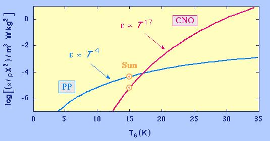
55 ppi cycle strongest at low T burning occurs throughout the core ppii cycle increases with T more important in central core ppiii cycle increases fastest with T most important in very center Finally, a byproduct of these reactions are the solar neutrinos. By incorporating the nuclear physics described above into the solar model, the following fluxes at earth are found (from Bahcall and Pinnsoneault 1995), in units of cm 2 s CNO Cycles Eν max (MeV) Flux p + p d + e + + ν e E10 8 B 8 Be + e + + ν e E6 7 Be + e 7 Li + ν e 0.86(90%) 4.89E9 0.38(10%) p + e + p d + ν e E8 Stars formed from the ashes of previous generations of stars will contain elements not produced in the big bang. As we have seen that charged particle reactions are suppressed by Coulomb barriers, the most interesting of these for helping to burn hydrogen at low temperatures are the lightest candidates. Carbon, nitrogen, and oxygen are the abundant, low Z, nonprimordial elements that one would first consider. These elements are produced by nuclear burning cycles in heavier stars and can be ejected into the interstellar medium through supernova explosions, stellar winds, etc. In stars somewhat heavier than our sun, higher temperatures and densities are produced in the core when the star first achieves radiative equilibrium. If metals are present, hydrogen burning can be achieved more efficiently through the pp cycle by a faster process involving proton capture on heavier elements. The cycle that dominates at the lowest temperatures is 12 C + p 13 N + γ 44

56 13 N 13 C + e + + ν e (τ 870 s) 13 C + p 14 N + γ 14 N + p 15 O + γ 15 O 15 N + e + + ν e (τ 178 s) 15 N + p 12 C + 4 He The important features of this cycle are It burns 4p 4 He, just as the pp cycle does. The heavy nuclei are neither produced nor consumed. They are analogous to deuterium and 3 He in our pp discussion. But this CN cycle requires some initial concentration of the heavy elements to turn on. In this regard these metals are not like the pp cycle s d, 3 He. The cycle will clearly burn to equilibrium in the metals, which can affect the relative portions of the metals. But this is only a redistribution: no new heavy elements are created. The two β decay reactions are relatively fast. Thus when a temperature is reached where the proton capture reactions proceed readily, the cycle can be quite fast. In our sun the total abundance by mass of elements with A greater than 5 is With this significant metallicity, the CN cycle accounts for a nonneglible amount of the 4 He synthesis, somewhat less than 2%. Under similar conditions but with the temperature elevated to T 7 1.8, the CNO cycle would begin to overtake the pp chain in importance. ThefactthattheCNcycleistakingoveratT means, in our sun, that one will not reach conditions where the ppiii cycle is primarily responsible for hydrogen burning. 45

57