Transcription

1

2

3

4

5

6

7

8

9

10

11

12

13

14

15

16

17

18

19

20

21

22

23

24

25

26

27

28

29

30

31

32

33

34 Hierdie vraestel bestaan uit 4 bladsye plus n bylae met formules (pp. i en ii). Hierdie vraestel bly die eiendom van die Universiteit van Suid-Afrika en mag nie uit die eksamenlokaal verwyder word nie. BEANTWOORD AL DIE VRAE. Vraag Explain the difference between a deterministic simulation model and a stochastic simulation model. Give an example of a real life system which requires development of a stochastic model for its description. (2) 1.2 A sequence of random numbers has two important statistical properties: uniformity and independence. Name two statistical tests for uniformity and two statistical tests for independence. (4) 1.3 Consider a random variable X with the following probability density function: { ax 3 if x [0,1] f(x) = 0 otherwise. Prove that a = 4. Suggest a procedure for generating a random number R from the distribution of the random variable X. (7) [13] [BLAAI OM]

35 2 DSC3703 Oct/Nov 2011 Vraag 2 Rupert sells daily newspapers on a street corner. Each morning he must buy the same fixed number Q of copies at R4 each. He sells them for R7 each through the day. He has noticed that the demand D during the day is close to being a random variable X that is normally distributed with mean µ = 135,7 and standard deviation σ = 27,1, except that D must be a nonnegative integer to make sense. So, D = max{[x]; 0} where [x] is the nearest integer to x. It is also assumed that demands from day to day are independent. Any unsold papers are returned to the publisher for a credit of R2 each. Any unsatisfied demand is estimated to cost R3 per paper in loss of goodwill and profit. Each day starts afresh, independent of any other day. 2.1 Prove that Rupert s profit is given by (2) Profit = 7min{Q; D} + 2max{Q D; 0} 3max{D Q; 0} 4Q. 2.2 Generate the daily demands D 1 and D 2 for two days by sequentially using the U(0; 1) random numbers as given in Appendix A. Show all the steps of the solution (6) 2.3 Assume that Q = 145. Determine the profit for two days with demands D 1 = 139 and D 2 = 154 given in subquestion 2. (2) 2.4 A simulation model for this problem is run for consecutive days for order quantities Q = 100;120;130;140 and 150 respectively. The computer output is given in the table below. Assume that Rupert wants to choose one of these values. Which one would you advise him to take. Substantiate your answer. Also find a 95% confidence interval for the profit for an order quantity of 160. Name Profit Profit Profit Profit Profit Profit Description (Sim#1) (Sim#2) (Sim#3) (Sim#4) (Sim#5) (Sim#6) Order Quantity Minimum Maximum Mean 275,35 307,61 328,43 337,71 336,80 328,03 Std Deviation 60,91 64,67 76,27 91,78 106,75 118,57 (6) [16] [BLAAI OM]

36 3 DSC3703 Oct/Nov 2011 Vraag 3 Five identical machines operate independently in a small shop. Each machine is up (that is, works) for between 6 and 10 hours (uniformly distributed) and then breaks down. There are two repair technicians available, and it takes a technician between 1 and 3 hours (uniformly distributed) to fix a machine; only one technician can be assigned to work on a broken machine even if the other technician is idle. If more than two machines are broken down at a given time, they form a virtual first-in-first-out repair queue and wait for the first available technician. A technician works on a broken machine until it is fixed, regardless of what else is happening in the system. All uptimes and downtimes are independent of each other. Assume that in the beginning all machines are working. This system can be modelled as a queuing system, by considering the machines as customers and the repair technicians as servers. Consider the following variables: TM is the clock time of the simulation, AT is the scheduled time of the next breakdown, DT is the scheduled time of the next repair completion, DT1 is the scheduled time for the next repair completion from Technician 1, DT2 is the scheduled time for the next repair completion from Technician 2, WL is the number of machines waiting in the queue, IT is the time between breakdowns, ST is the service time (time to complete a repair), SS1 is the status of Technician 1 (0 for idle and 1 for busy), SS2 is the status of Technician In building a simulation model for this system, what events should be considered? (2) 3.2 After what time should the technicians expect the first breakdown to happen? Substantiate your answer. (2) 3.3 Give the initial values of the variables TM, DT, DT1, DT2, WL, SS1 and SS2. (3) 3.4 Generate 5 random times at which the first 5 breakdowns will happen and generate corresponding 5 random service times using sequentially the U(0; 1) numbers given in Appendix A (Use U 1 ;...;U 5 to generate the breakdown times and U 6 ;...;U 10 for the service times). At which time will the repair of machine 2 be completed? How much time will machine 4 spend in the queue? Substantiate your answers. (9) [16] [BLAAI OM]

37 4 DSC3703 Oct/Nov 2011 Vraag 4 Parts arrive at a single workstation system according to an exponential interarrival distribution with mean 60 seconds; the first arrival is at time 0. Upon arrival, the parts are processed on a machine. The processing time is a random variable with triangular distribution TRIANG(18;19;22) seconds (that is a = 18;c = 19;b = 22). Assume that the model will be run for 1000 seconds. 4.1 Develop a simulation model for this system. (12) 4.2 Run your model until the first part leaves the system. You should sequentially use the U(0; 1) random numbers as given in Appendix A to generate random numbers from other distributions. Clearly define all variables used. (16) Vraag 5 [28] The following algorithm can be used to generate random numbers from a gamma distribution with parameters α (0;1) and β = 1. Apply it to generate one random number from a gamma distribution with α = 0,5 and β = 1. You may sequentially use the U(0; 1) random numbers given in Appendix A when necessary. Found:= false; b := (e + α)/e; {Comment: use e 2,718} while Found = false do Generate U 1 U(0,1) P := bu 1 if P > 1 then Y := ln[(b P)/α]; Generate U 2 U(0; 1); if U 2 Y (α 1) then Found = true; Return Y ; end if; else Y = P 1/α ; Generate U 2 U(0;1); if U 2 e Y then Found = true; Return Y ; end if end if end while (7) [7] TOTAAL: 80 c UNISA 2011

38 i DSC3703 Oct/Nov 2011 BYLAE A Formules en getalle Kansgetalle Die volgende ry van 20 kansgetalle is opeenvolgend uit n U[0;1)-verdeling gegenereer. U 1 = 0,56 U 9 = 0,15 U 17 = 0,81 U 25 = 0,69 U 33 = 0,78 U 2 = 0,31 U 10 = 0,09 U 18 = 0,63 U 26 = 0,68 U 34 = 0,92 U 3 = 0,67 U 11 = 0,40 U 19 = 0,87 U 27 = 0,60 U 35 = 0,19 U 4 = 0,80 U 12 = 0,78 U 20 = 0,46 U 28 = 0,20 U 36 = 0,56 U 5 = 0,97 U 13 = 0,15 U 21 = 0,96 U 29 = 0,26 U 37 = 0,86 U 6 = 0,73 U 14 = 0,04 U 22 = 0,92 U 30 = 0,71 U 38 = 0,73 U 7 = 0,15 U 15 = 0,58 U 23 = 0,80 U 31 = 0,13 U 39 = 0,42 U 8 = 0,51 U 16 = 0,13 U 24 = 0.33 U 32 = 0,92 U 40 = 0,54 Die chi-kwadraattoetswaarde χ 2 = k n k (f j n k )2 j=1 Persentielpunte van die chi-kwadraatverdeling Vryheidsgrade (d.f.) α ν 0,95 0,90 0,10 0,05 3 0,35 0,58 6,25 7,81 4 0,71 1,06 7,78 9,49 5 1,15 1,61 9,24 11,07 6 1,64 2,20 10,64 12,59 7 2,17 2,83 12,02 14,07 8 2,73 3,49 13,36 15,51 9 3,33 4,17 14,68 16, ,94 4,87 15,99 18,31 Die Kolmogorov-Smirnovtoetswaardes ,85 15,66 33,20 36,42 [ ] i D + = max 1 i n n F X(x (i) ) [ D = max F X (x (i) ) i ] 1 i n n D = max(d + ;D ) T = D( n + 0,12 + 0,11/ n) Persentielpunte vir T: Persentasie ,5 1 Kritieke waarde 1,138 1,224 1,358 1,480 1,628

39 ii DSC3703 Oct/Nov 2011 Kumulatieweverdelingsfunksies { 1 e (x/β) as x 0 Eksponensiaalverdeling: F(x) = 0 andersins { 1 e (x/β) α as x > 0 Weibull-verdeling: F(x) = 0 andersins 0 as x < a x a Uniforme verdeling: F(x) = b a as a x b 1 as x > b 0 as x < a (x a) 2 (b a)(c a) as a x c Driehoekige verdeling: F(x) = 1 (b x)2 (b a)(b c) as c < x b 1 as x > b Vertrouensintervalle en die t-verdeling n 100(1 α)%-vertrouensinterval vir E(X) word gegee deur waar X = n i=1 X ± t (α/2;n 1) S 2 X i n S 2 = n n (X i X) 2 i=1 n 1 Persentielpunte van die t-verdeling Sentralelimietstelling Vryheidsgrade (d.f.) α ν 0,1 0,05 0,025 0,01 1 3,078 6,314 12,706 31, ,886 2,920 4,303 6, ,638 2,353 3,182 4, ,533 2,132 2,776 3, ,476 2,015 2,571 3, ,440 1,943 2,447 3, ,415 1,895 2,365 2, ,397 1,860 2,306 2, ,383 1,833 2,262 2, ,281 1,645 1,960 2,326.. Die som van n onafhanklike en identies verdeelde kansveranderlikes, elk met n gemiddelde µ en eindige variansie σ 2, is benaderd normaal verdeel met gemiddelde nµ en variansie nσ 2....

40 -i- DSC3703 Oct/Nov 2011 Memorandum VRAAG A deterministic simulation model contains no random variables whereas a stochastic simulation model contains one or more random variables. A queuing system where entities arrive randomly or the service time is random is example of a real life system which requires development of a stochastic model for its description. (2) 1.2 The Chi-square goodness-of-fit and the Kolmogorov-Smirov goodness of fit tests are suitable to test the uniformity of random numbers. The runs-up and lag-j correlation tests are suitable for independence. (4) 1.3 We know that f is a pdf then f(x)dx = 1. Then we find (7) f(x)dx = 1 0 ax 3 dx = a/4 and hence a = 4. The cumulative distribution function of X is given by F(x) = x f(t)dt Then 0 if x < 0 F(x) = x 4 if 0 x 1 1 if x > 1 The following algorithm generates a random number from that distribution. Generate U U(0; 1) Return R = F 1 (U) = U 1/4. [13] VRAAG We have that Profit = Revenue - Total costs. There are two possible cases: If Q D, then Rupert sells all the Q papers and receives 7Q rands. He pays 4Q to buy the papers and looses 3(D-Q) for unsatisfied demand. If Q D, then Ruperts sells only D papers and receive 7D rands and he receives 2(Q D) from the returned papers (to the publishers). With the the order costs of 4Q rands, it is clear that in both cases the equation is satisfied. 2.2 It is given that D has a normal distribution with mean µ = 135,7 and standard deviation σ = 27,1. Then we can generate random numbers by using one of the appropriate algorithms (2) (6) Memorandum i Blaai om asseblief

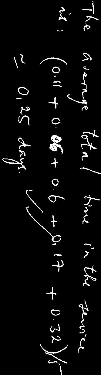
41 -ii- DSC3703 Oct/Nov 2011 described in the study guide. The simplest is the following simplified convolution algorithm Generate U i U(0; 1), i = 1,...,36. Consider Z 1 = U U 12 6; Z 1 = U U 24 6; Consider X i = µ + σz i. Return D i = max([x i ],0), i = 1,2 Using the algorithm, we find Z 1 = 0,12;Z 2 = 0,68 and D 1 = 139;D 2 = The profits corresponding to these demands are R405 and R408 respectively 2.4 One can advise Rupert to choose the order quantity of 150 because it gives the highest mean profit. But the order quantity of 140 can also be considered for a small risk compared to 140. (2) (6) The 95% confidence interval for the profit (if Q = 160) is given by Mean profit ± t (0.025,9999) mean standard error and mean standard error = standard deviation = 106,75/100 = 1,0675. number of iteration Noting that t (0.025,9999) = 1,9602 we find the interval [334,71; 338,90] [16] VRAAG The three main events are: a break down (that is an arrival of a new machine), a departure (or completion of repair) from Technician 1 and a departure from Technician Because the life time of a machine is U(6,10) hours, then the first breakdown is expected at time t = (6 + 10)/2 = 8 hours. 3.3 The initial values of the given variables are: TM = 0, DT,DT1,DT2 can be taken to be any large number, WL = 0; SS1 = SS2 = We use the following algorithm to generate random numbers from U(a; b): Generate U U(0; 1) Return X = a + (b a)u For the breakdown times, we find (using random numbers U 1,...,U 5 ) X 1 = 8,24;X 2 = 7,24;X 3 = 8,68;X 4 = 9,20;X 5 = 9,88 (2) (2) (3) (9) and for services times using U 6,...,U 10 ), Y 1 = 2,46;Y 2 = 1,30;Y 3 = 2,02;Y 4 = 1,30;Y 5 = 1,18. Memorandum ii Blaai om asseblief

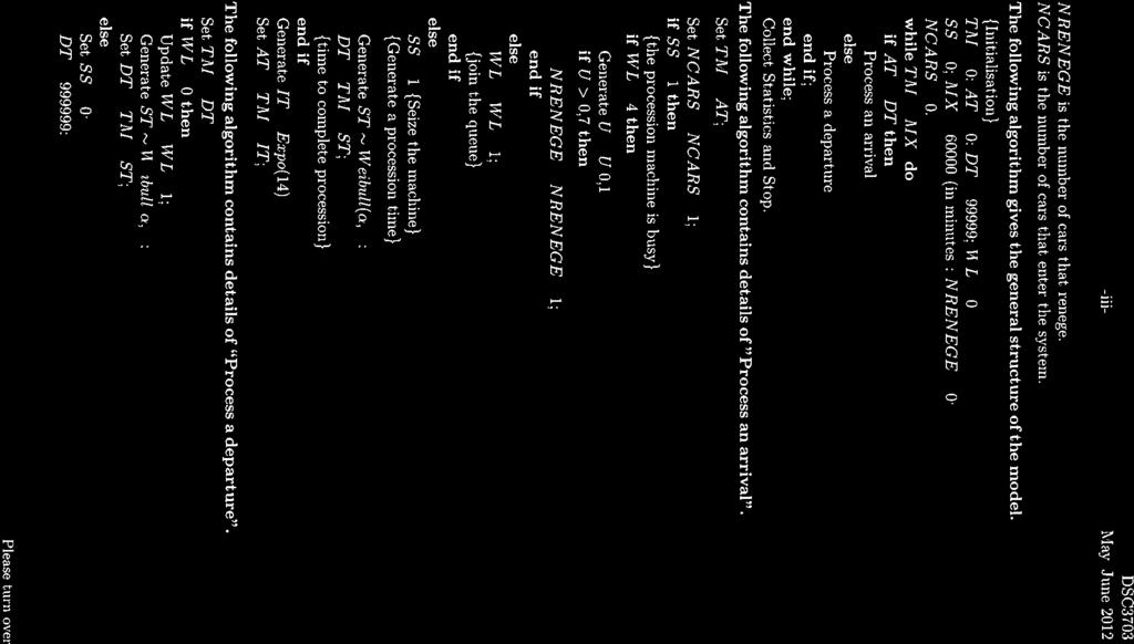
42 -iii- DSC3703 Oct/Nov 2011 Machine 2 will break down at time TM = 7,24 and its repair will start immediately and will be completed at TM = 7,24 + 1,30 = 8,54. Machine 1 will break down at TM = 8,24 and it repair will start immediately and end at TM = 8,24 + 2,46 = 10,70. Machine 3 will break down at time TM = 8,68 and there is a technician available to repair it. So its repair will be completed at TM = 8,68 + 2,02 = 10,70. Machine 4 will break down at T M = 9,20 while both technicians are busy. Its repair will only start at TM = 10,70 and will be completed at TM = 10,70 + 1,18 = 11,88. So the time Machine 4 will spend in the queue is 10,70 9,20 = 1,5. [16] VRAAG The following variables may be used: TM is the clock time of the simulation, AT is the scheduled time of the next arrival, DT is the scheduled time of the next procession completion, WL is the number of parts waiting in the processing queue, IT is the interarrival time, ST is the service time for procession, SS is the status of the procession machine (0 for idle and 1 for busy), MX length of the simulation run, The following algorithm can be used to model the system: {Initialisation} TM = 0; AT = 0; DT = 1000; WL = 0 ; SS = 0; MX = 1000 while TM MX do if AT DT then {process an arrival of a part} Set TM = AT if SS = 1 then {the procession machine is busy} WL = WL + 1; {join the queue} else {the procession machine is idle} SS = 1 {Seize the machine} {Generate a procession time} Generate ST TRIA(16,19,22) ; DT = TM + ST; {time to complete procession} end if; Generate IT EXPO(60) Set AT = TM + IT; else if AT > DT then {process a departure from procession} (12) Memorandum iii Blaai om asseblief

43 -iv- DSC3703 Oct/Nov 2011 Set TM = DT if WL > 0 then Update WL = WL 1; Generate ST T RIAN G(18,19,22); Set DT = TM + ST; else Set SS = 0; DT = 1000; end if; end if; end while; Print results and STOP. 4.2 To run the algorithm, proceed as follows : Iteration 1: We start with TM = 0 and TM MX is satisfied. The condition AT DT is also satisfied. We check the condition SS = 1, which is false. Set SS = 1 Then we generate a service time ST TRIA(16,19,22). {The following procedure can be used to generate random numbers from T RIA(a,c,b)}: Generate U U(0; 1) Set c = (c a)/(b a) if U c then X = c U else X = 1 (1 c )(1 U) end if; Return Y = a + (b a)x Now to find ST we take c = 0,5 and U = 0,56. Then U > c. Then X = 1 (1 c )(1 U) = 0,53 And Y = ,53 = 19,18 Then ST = 19,18; DT = TM + ST = 19,18 Generate IT EXPO(60). {The following procedure generates random numbers from EXPO(β):} Generate U U(0; 1) Return Y = β ln(1 U) Take U = 0,31 and return IT = 60 ln(1 0,31) = 22,26 Set AT = TM + IT = ,26 = 22,26. The first itreation is completed. Iteration 2: We have TM = 0, AT = 22,26;DT = 19,18; MX = 30,SS = 1 The condition TM MX is true. The condition AT > DT is true. (16) Memorandum iv Blaai om asseblief

44 -v- DSC3703 Oct/Nov 2011 {process a departure} The condition WL > 0 is false {the que is empty} Set SS = 0 and DT = The first part has left the system. STOP [28] VRAAG First consider b = (2, ,5)/(2,718) = 1,184 and U 1 = 0,56 Set P = b U 1 = 1,184 0,56 = 0,663 Since P > 1 is false, then Set Y = P 1/α = (0,663) 2 = 0,44. Generate U 2 = 0,31 e Y = 0,644 and hence U 2 e Y is true. Found = true (7) Return Return Y = 0,44. [7] TOTAAL: 80 Regmerke: 80 Antwoordpunte: 80 Memorandum v

45

46

47

48

49

50

51

52

53

54

55

56

57

58

59

60

61

62

63

64

65

66

67

68

69

70