Inference in Regression Model

Transcription

1 Inference in Regression Model Christopher Taber Department of Economics University of Wisconsin-Madison March 25, 2009

2 Outline 1 Final Step of Classical Linear Regression Model 2 Confidence Intervals 3 Hypothesis Testing 4 Testing Multiple Hypotheses at the same time 5 Examples

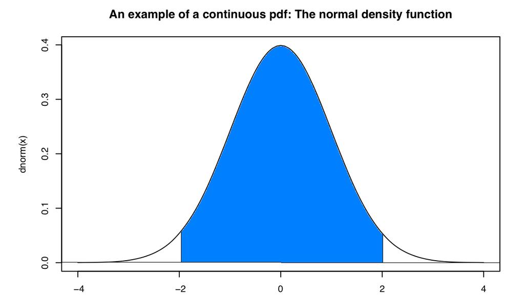
3 Normality Assumption We need to add one more assumption to get the final part of the Classical Linear Regression Model Assumption MLR 6 (Normality) The population error u is independent of the explanatory variables x 1, x 2,..., x k and is normally distributed with zero mean and variance σ 2 : u N(0, σ 2 )

4 What do you think of this assumption? It is awfully strong-why should we believe the error term is normally distributed? Many distributions look like bell curves but that does not necessarily mean normality is a good assumption. When we worry about OLS asymptotics we will see a better way of handling this problem

5 Why is this assumption useful? Remember the simple regression model ˆβ 1 = β 1 + N i=1 (x i x)u i N i=1 (x i x) 2 This is a linear combination of normal random variables so it is normally distributed.

6 Putting the assumption into action gives the following result Theorem 4.1 (Normal Sampling Distributions) Under the CLM assumptions MLR.1 through MLR.6, conditional on the sample values of the independent variables ˆβ j N(β j, Var( ˆβ j )), where Var( ˆβ j ) was given in Chapter 3 [equation(3.51)]. Therefore, ( ˆβ j β j ) sd( ˆβ j ) N(0, 1).

7 We never actually looked at equation 3.51 in the lecture notes, so let me give it now Theorem 3.2 (Sampling Variance of the OLS Slope Estimators) ( ) σ 2 Var ˆβ j = ) SST j (1 Rj 2 for 1, 2,..., K where SST j = N ( ) 2 i=1 xij x j is the total sample variation in x j, and Rj 2 is the R-squared from regression x j on all other independent variables (and including an intercept).

8 A fly in the Ointment This is all fine, except for one thing We don t know σ 2! We can estimate it in the way you might expect (well close to it) ˆσ 2 = 1 N K 1 N ûi 2. i=1 This turns out to be an unbiased estimate of σ 2. We define the standard error of ˆβ j as ( ) se ˆβ j = ˆσ 2 ) SST j (1 Rj 2

9 Then we have the result that Theorem 4.2 (t Distribution for the Standardized Estimators) Under the CLM assumptions MLR.1 through MLR.6, ˆβ j β j se( ˆβ j ) t N K 1 where K + 1 is the number of unknown parameters in the population model y = β 0 + β 1 x β k x k + u (K slope parameters and the intercept β 0 ). Now we don t know β j, but this won t be particularly important for what we are doing. Note as well that if N-K-1 is large then the t-distribution is almost identical to the normal distribution

10 How is this all useful? Lets forget about regression now and think more generally about inference. We have talked about how to construct regression estimators and their distribution, but not about statistical inference. It will turn out that you already learned how to do this in your Statistics class. Lets first think about why we care

11 Example 1 You want to decide whether to be a doctor or a lawyer. You have a sample of earnings of people in the population For Doctors Y = $123, 452 For Lawyers Y = $112, 935 Should you be a doctor or a lawyer? How confident are you?

12 Example 2 Batting Averages: You go to one basketball game Charlie Villenueva scores 32 points Lebron James scores 17 points Who is a better?

13 Example 3 You are a firm thinking about switching to a new mode of production. It saves about $1100 on average, but costs $1000. Should you buy it?

14 Example 4 You are trying to predict the stock market. You think unemployment might be important. You run a regression of stock gains on unemployment and find b 2 = Should you necessarily invest all your money in the stock exchange? You would like to test formally whether b 2 > 0.

15 Example 5 You want to know whether crime in Chicago is related to the temperature. You run a regression where A t : Arrests in Chicago at date t T t : Temperature in Chicago at date t You find that A t = T t + ε t It looks like there are more arrests when the temperature is higher, but are you sure?

16 Example 6 You are interested in how much cars depreciate. You have information on their age and their price. P i : Price of car i in $1000 A i : Age of car i P i = A i + ε i How do you interpret this? How confident are you?

17 Outline 1 Final Step of Classical Linear Regression Model 2 Confidence Intervals 3 Hypothesis Testing 4 Testing Multiple Hypotheses at the same time 5 Examples

18 Lets forget about regression or sample means or anything else and just assume that we have some estimator θ that is a function of the data. This estimator is normally distributed and is an unbiased estimate of θ. θ N ( ) θ, σθ 2

19 Lets also not worry about T distributions for now, but assume that N K 1 is large enough that the distribution is approximately normal. There is a little trick with normal random variables that makes them easy to deal with. What is the distribution of θ θ σ θ?

20 First note that θ and σ θ are nonstochastic while θ is normally distributed. Therefore this must be normally distributed. If we know its expectation and we know its variance we know everything there is to know about it.

21 E ( ) θ θ σ θ = 1 ) ) (E ( θ θ σ θ = 0 Var ( ) θ θ σ θ ( 1 = var ( θ )) θ σ θ = 1 ) σθ 2 var ( θ = σ2 θ σ 2 θ = 1

22 This means that θ θ σ θ N (0, 1) This is true for any normally distributed random variable.

23 The distribution N(0, 1) is called a standard normal You can find tables in the back of the book that gives its distribution. What the tables will show is that for any variable, say Z, that is a standard normal Pr ( 1.96 Z 1.96) = 0.95 That is 95% of the time a standard normal random variable will lie between and 1.96.

24 This is true for any standard normal so it has to be true for b θ θ σ θ, thus Pr ( 1.96 θ ) θ 1.96 σ θ = 0.95 Now after doing some algebra, we will get a nice expression.95 = Pr( 1.96 θ θ σ θ 1.96) = Pr( 1.96σ θ θ θ 1.96σ θ ) = Pr( 1.96σ θ θ θ 1.96σ θ θ) = Pr( 1.96σ θ + θ θ 1.96σ θ + θ) We call this a 95% confidence interval.

25 If you construct it in this way, it will cover the true θ 95% of the time. It is important to remember that what is random here is θ and not θ. Thus it is the interval that is random, not the variable inside it.

26 Constructing a Confidence Interval for the expected value of a Normal Distribution Let s start with the case of Y i N(µ Y, σ 2 Y ) and Y i and Y j are independent for i j, so cov(y i, Y j ) = 0. The sample mean Y is Y = 1 N N i=1 Y i Y is a random variable; what is its distribution?

27 Since it is a linear combination of normal random variables, it s normal. Its mean is E(Y ) = µ Y Its variance is Var(Y ) = σ2 Y N

28 The standard error of an estimator is its standard deviation (i.e. the square root of its variance), so we also have: se(y ) = σ Y N Thus Y N ( µ Y, σ2 Y N ) This is just a special case of what we learned above with Y taking the place of θ and µ Y taking the place of θ. Thus Pr( 1.96 σ Y N + Y µ Y 1.96 σ Y N + Y )

29 Confidence Intervals for Regression Coefficients Now we want to construct confidence intervals for regression coefficients. Once again these are just special cases of θ. Take β 1 : ˆβ 1 N(β 1, Var( ˆβ 1 )), Now β 1 takes the place of θ and ˆβ 1 takes the place of θ so that.95 = Pr( 1.96se( ˆβ 1 ) + ˆβ 1 β se( ˆβ 1 ) + ˆβ 1 ) Similarly for any of the other regression coefficients.95 = Pr( 1.96se( ˆβ j ) + ˆβ j β se( ˆβ 1 ) + ˆβ 1 ) Lets look at some examples

30 Our first example is from the RDCHEM data set. Lets just try the simple regression of profits on Research and Development expenditure We find that ˆβ 1 = ( ) se ˆβ1 = N = 32 K = 1 We want to construct a 95% confidence interval. N-K-1=30

31 The critical value for a 2-tailed T test with 30 degrees of freedom is The confidence interval is ( 2.042se ( ˆβ 1 ) + ˆβ 1, 2.042se ( ˆβ 1 ) + ˆβ 1 ) = ( , ) = (2.146, 2.728) Which is what stata shows.

32 Now consider a regression of the hours worked in a year Lets think about a 95% confidence interval for the hourly wage ˆβ 1 = ( ) se ˆβ1 = N = 428 K = 5 This gives us 422 degrees of freedom which is large enough that this is approximately normal

33 ( ) ( ) ( 1.96se ˆβ 1 + ˆβ 1, 1.96se ˆβ 1 + ˆβ 1 ) = ( , ) = ( 45.12, 0.84)

34 Next lets get a 90% confidence interval for the number of kids less than 6. Again we will be approximately normal, but for a 10% interval the critical value is ( ) ( ) ( 1.645se ˆβ 4 + ˆβ 4, 1.645se ˆβ 4 + ˆβ 4 ) = ( , ) = ( , ) Note that this is smaller than the 95% interval That makes sense

35 Outline 1 Final Step of Classical Linear Regression Model 2 Confidence Intervals 3 Hypothesis Testing 4 Testing Multiple Hypotheses at the same time 5 Examples

36 Hypothesis Testing First lets think more generally what Hypothesis testing is and then worry about statistical inference Let H 0 be some hypothesis that you want to test. Suppose that it is true. We then ask whether the world seems consistent with it. Specifically: we perform some experiment and see if the results of the experiment are consistent with the hypothesis

37 Examples 1 There is no gravity 2 I only have one set of keys and I left them in the car 3 I always wear socks We can easily design experiments and test these hypotheses

38 In statistics life isn t so easy We can almost never reject for sure That is we very rarely know for sure that the null is definitely wrong For example, consider the hypothesis H 0 : µ x = 0 Even if x = it is still possible (although unlikely) that the true value is 0

39 In doing hypothesis testing we formalize these ideas We must deal with the following: Type 1 error=α = Probability of rejecting H 0 even when it is true We would like this to be zero, but it statistics it generally can not be

40 Now we need to construct a test statistic that has to have two features: 1 Depends on the data in a known way 2 We know its distribution when the null hypothesis is true We then choose an acceptance region A so that when t / A we reject the null hypothesis We choose A in such a way that Pr(reject H 0 H 0 true) = α

41 Lets look at some examples

42 Example 1: Probability of Getting a Job Suppose you are out trying to get a job and you think that the probability of getting a job offer is one half. That is H 0 : Pr (J) = 0.5 Now you go out and interview with a bunch of different firms until you get a job. You want to test the null hypothesis that the probability of getting a job was really 0.5 depending on how long it takes you to find one Lets define a test statistic t to be the number of jobs for which you interview until you get one

43 Is this a legitimate test statistic? It depends on the data. I know its distribution when the null hypothesis is true

44 To see the last part notice that Prob. Job after 1 interview 0.5 Prob. Job after 2 interviews 0.25 Prob. Job after 3 interviews Prob. Job after 4 interviews Prob. Job after 5 interviews Prob. Job after more than 5 interviews

45 How do we do this? Set α = and choose our acceptance region A = {1, 2, 3, 4} Thus we reject when we reach our fifth interview Probability of getting to fifth interview = Probability of being rejected after 4 interviews = = α

46 Example 2: Sample Mean Suppose x i N ( ) µ x, σx 2 Take the null hypothesis to be that µ x is some particular value, H 0 : µ x = x Now set t = x x ŝe( x)

47 Does this satisfy our criteria? It depends on the data. We know x and we can estimate x and ŝe( x). We know its distribution under the null hypothesis. Under the null x i N(x, σ 2 x) So we know that x N ( ) x, σ2 x N and from statistics class you learned that t T N 1 (that is a T distribution with N-1 degrees of freedom)

48 Example 3: Regression Coefficient Suppose we want to test something about β 1. In particular suppose we want to test that H 0 : β 1 = β 1

49 What should we use as our test statistic? It needs to depend on the data. That is given a set of X s and Y s, I need to be able to get the test statistic I need to know its distribution under the null hypothesis. We know that under the assumption of the classical linear regression model and under the null hypothesis ˆβ 1 N(β 1, se( ˆβ 1 ) 2 ) so and ˆβ 1 β 1 se( ˆβ 1 ) t = ˆβ 1 β 1 se( ˆβ 1 ) N(0, 1) T N K 1

50 There is still an issue we have not dealt with at all We have talked about how hypothesis testing works and what we need to do it. However, we have not talked at all about how we choose the acceptance region At this point anything will work as long as the probability of rejection is α. In particular if we know that our distribution is T N K 1 there are many ways to choose the region that will work. How do we choose the right one?

51

52

53

54

55 Power Our main criterion for picking the right region is β = Pr(Reject H 0 H 0 false) We want to choose the region so that fixing the size= α, the power is as large as possible Lets focus on the null hypothesis that β 1 = 0 Suppose in reality that the null is false and that instead β 1 = 3

56 What is the distribution of the test statistic under this alternative? t = = ˆβ 1 se( ˆβ 1 ) 3 se( ˆβ 1 ) + ˆβ 1 3 se( ˆβ 1 ) 3 + T N K 1 se( ˆβ 1 ) This is going to be a T distribution shifted to the right.

57 Lets think about the following four 95% acceptance regions A = { 1.96 t 1.96} B = {t 1.64} C = { 1.64 t} D = {t 0.06, t 0.06} Assuming that N-K-1 is large so this is approximately normal, all 4 have the same size α = 0.05.

58 That is under the null hypothesis Pr(A H 0 ) = Pr ( 1.96 t 1.96 H 0 ) = 0.95 Pr(B H 0 ) = Pr (t 1.64 H 0 ) = 0.95 Pr(C H 0 ) = Pr ( 1.64 t H 0 ) = 0.95 Pr(D H 0 ) = Pr (t 0.06, t 0.06 H 0 ) = 0.95

59

60

61

62

63 For this example which region gives us the most power? Answer: region B What about if under the alternative β 1 = 3? Region C What if you are not really sure whether β 1 is positive or negative under the null? Then you would probably choose region A. Would you ever choose D? Not for any reason I can think of Lets look at a couple of examples.

64 Cigarette Smoking Do a higher price of cigarettes lead people to smoke less? We can write the null hypothesis as H o : β 1 = 0 The interesting alternative is β 1 < 0 so it makes sense to use a one sided test. N-K-1 is large enough that we will use the normal distribution (degrees of freedom= )

65 Thus the critical value is We reject if We fail to reject the null >T = = 0.32 Alternatively we could use a two-sided test. Then we reject if t < 1.96 or if t > 1.96 We don t reject either of these

66 We can also try a one-sided test at the 10% level The critical value here is We are still nowhere close You can see from stata that the p-value is You would never use one that large

67 Wine and Death Lets look at the relationship between wine consumed and death. Here you would not really know what to think, so a two sided test makes more sense. We have 21 observations so the degrees of freedom is 19. This gives the critical value of a 95% test at Calculate We fail to reject the null. t = = 1.98

68 What about a 90% test. In that case the critical value is Again we can look at the p-value which is This means that we would reject a test of size we would fail to reject with a size of 0.061

69 Even if you reject the null does that mean that you should drink a lot of wine? Suppose (and I do not know the exact numbers but am making them up), you can either drink wine or drink vitamin water Say that the doctor tells you drinking vitamin water will save 30 lives per 100,000 Is drinking wine as effective?

70 The null hypothesis now is β 1 = 30 The test statistic is now t = ˆβ se( ˆβ 1 ) = 8.20 = 1.68 The critical values are the same as before so we fail to reject the null both at the 5% and 10% level

71 Testing linear combination of parameters Sometimes we want to test more complicated tests about more than parameters at once One really nice example is work by Kane and Rouse They want to ask, what is worth more, a year in community college or a year at a four year college. They look at the regression log(wage) i = β 0 + β 1 jc i + β 2 univ i + β 3 exper i + u i where jc i is the number of years of junior college while univ i is the number of years of university training and exper i is experience.

72 It is interesting to test the null hypothesis H o : β 1 = β 2 How do we do this? Note that we can write this as H o : β 1 β 2 = 0 Now it looks a bit like what we did before

73 Remember that ˆβ 1 ˆβ 2 is a sum of normal random variables, so it is normal ( ) E ˆβ 1 ˆβ 2 = β 1 β 2 ( var ˆβ1 ˆβ ) ( ) ( ) ( 2 = var ˆβ1 + var ˆβ2 2cov ˆβ1, ˆβ ) 2 Thus under the null hypothesis ˆβ 1 ˆβ 2 ( ) N(0, 1) var ˆβ 1 ˆβ 2

74 and when we deal with the fact that we estimate the standard error ˆβ 1 ˆβ 2 var ( ˆβ 1 ˆβ 2 ) T N K 1

75 There is no easy way to do this in stata, but there are two other ways to do it. The first way is to redefine the model slightly. What we care about testing is β 1 β 2 so lets define Also define θ 1 = β 1 β 2. totcol = jc + univ which is just the total number of years of college that a person has.

76 Then think about the population regression function log(wage) i = β 0 + β 1 jc i + β 2 univ i + β 3 exper + u i = β 0 + (θ 1 + β 2 ) jc i + β 2 univ i + β 3 exper + u i = β 0 + θ 1 jc i + β 2 (jc + univ i ) + β 3 exper + u i = β 0 + θ 1 jc i + β 2 totcol + β 3 exper + u i This gives us a nice way of testing the restriction It also makes sense intuitively.

77 Outline 1 Final Step of Classical Linear Regression Model 2 Confidence Intervals 3 Hypothesis Testing 4 Testing Multiple Hypotheses at the same time 5 Examples

78 The other test one might want to do is to test more than one null hypothesis at a time. For example in the previous example you might be interested in testing the joint null hypothesis H 0 : β 1 = 0 We don t know how to do this yet. β 2 = 0.

79 To get some intuition lets think about comparing a restricted regression model with the unrestricted model. Lets write the unrestricted model as log(wage) i = β u 0 + βu 1 jc i + β u 2 univ i + β u 3 exper i + u u i The restricted model is log(wage) i = β r 0 + βr 3 exper i + u r i. Under the null hypothesis these models are equivalent.

80 Intuitively If the null hypothesis is true the two models are the same. That means when we include jc i and univ i into the model, the sum of squared residuals should not change much. However, if the null hypothesis is false that means that at least one of β 1 or β 2 is nonzero and the sum of squared residuals should fall when we include these new variables. This seems like it could be the basis of a test.

81 If the sum of squared residuals changes a lot we reject the null hypothesis. It only makes sense to to this as a one sided test. It turns out it works the following statistic works. F = (SSR r SSR u ) /q SSR u /(N K 1)

82 Here q is the difference in degrees of freedom in the restricted model versus the unrestricted model Equivalently it is the number of restrictions that you are testing in the null hypothesis. In the case we are looking at, q = 2 Note that it increases with SSR r so we reject when it is a big number.

83

84 We call this an F distribution with q degrees of freedom in the numerator and N K 1degrees of freedom in the denominator. We can also write it in terms of R 2, F = (SSR r SSR u ) /q SSR u /(N K 1) ) /q = = ( SSRr SST SSR u SST SSRu SST /(N K 1) ( R 2 u Rr 2 ) /q ( ) 1 R 2 u /(N K 1)

85 This gives us a really easy way to test the joint hypothesis that all of the coefficients in the regression are zero other than the intercept. That is the null hypothesis H 0 : β 1 = β 2 =... = β K = 0. What is the R 2 in the restricted model? It has to be zero. Thus the test statistic for this regression is just F = R 2 /q ( 1 R 2 ) /(N K 1)

86 Now back to the two year college example. I said there was another way to do it. Well there is nothing that says you can t use an F-test when you only have one restriction (q = 1). For the community college model the restricted model would have β 1 = β 2 so we can write this as log(wage) i = β 0 + β 1 jc i + β 2 univ i + β 3 exper + u i = β 0 + β 1 jc i + β 1 univ i + β 3 exper + u i = β 0 + β 1 (jc i + univ i ) + β 3 exper + u i = β 0 + β 1 totcol + β 3 exper + u i

87 We have SSR u = SSR r = q = 1 N K 1 = 6760 Thus we get F = (SSR r SSR u ) /q SSR u /(N K 1) ( ) /1 = /6760 = 2.15 The critical value for an F-test with 1 degree of freedom in the numerator and in the denominator is 3.84 so we fail to reject the null hypothesis.

88 Relationship between F and T tests It turns out that this F-test is closely related to the t-test In fact the the t-statistic squared has an F distribution with 1 degree of freedom in the numerator. Note that = 3.84 the critical value of the F-test.

89 Testing in stata Stata does things slightly different than the way I presented it. Lets look at a number of examples

90 Outline 1 Final Step of Classical Linear Regression Model 2 Confidence Intervals 3 Hypothesis Testing 4 Testing Multiple Hypotheses at the same time 5 Examples

91 Example 1: Baseball Salaries Use the data mlb1 from Wooldridge First test the overall significance of the regression F = = R 2 /q ( 1 R 2 ) /(N K 1) /5 (0.3722) /(347) = You can see that stata did it for you already

92 Test whether the performance variables are jointly zero That is H 0 : β 3 = β 4 = β 5 = 0 Run the restricted model which gives an R 2 = Then you get F = ( R 2 u Rr 2 ) /q ( ) 1 R 2 u /(N K 1) = ( ) /3 (0.3722) /(347) = 9.54 The critical value is 2.6 so we reject

93 Example 2: Firm size and participation rate Lets look at the relationship between various things and participation rates in 401K plans Does type of plan matter? Does size of firm matter? Even though firm size is statistically significant it is not economically significant.

94 Example 3: The Death Penalty The death penalty is an extremely controversial policy Proponents claim it deters crime Opponents claim there is no evidence of this Lets look at the evidence using death.do and murder.raw Key variables: mrdrte exec murders per 100,000 population total executions, past 3 years

95 One conclusion from this is that there is no evidence that the death penalty deters crime In fact point estimates go other way, murder rises with executions

96 Therefore there is no argument for it This is exactly the type of argument about which one has to be very careful Just because a coefficient is insignificant doesn t mean it is zero Confidence interval is (-.218,.0.548) Lower bound is about -0.2 Interpreting this number as causal would mean that one execution every three years would save 0.2 lives for every 100,000 people each year

97 Lets try to figure out whether this is a big number or not The state of Illinois is about 12,000,000 That -0.5 would mean that every execution saves about lives 12, 000, , 000 This seems like a big number to me = 72

98 Can t reject that deterrent effect is zero Also can t reject that it is really powerful Also can t reject that is is really powerful, but goes in other direction In other words this analysis is completely uninformative I suspect gun control works in exactly the same way (but opposite politically)