Inference in Regression Analysis

Transcription

1 ECNS 561 Inference

2 Inference in Regression Analysis Up to this point 1.) OLS is unbiased 2.) OLS is BLUE (best linear unbiased estimator i.e., the variance is smallest among linear unbiased estimators) But, so far, we have not explored the sampling distribution of β j Under our Gauss-Markov assumptions, the sampling distribution can have virtually any shape Conditioning on Xs, our sampling distribution of the OLS estimators depend on the underlying distribution of errors To make the sampling distributions of the β j tractable, we assume the unobserved error is distributed normally.

3 Assumption MLR.6 Normality The population error ε is independent of the right-hand-side variables x 1, x 2,, x k and is normally distributed with zero mean and variance σ 2 : ε ~ Normal(0, σ 2 ) For cross-sectional regressions MLR.1-MLR.6 are called the classical linear model (CLM) assumptions We refer to this as the classical linear model Under the CLM assumptions, the OLS estimators have a stronger efficiency property than under the Gauss-Markov assumptions (MLR.1-MLR.5) It can be shown that the OLS estimators are the minimum variance unbiased estimators We no longer have to restrict our comparison to estimators that are linear in the y i Summarized as y x ~ Normal(β 0 + β 1 x β k x k, σ 2 ) i.e., conditional on x, y has a normal distribution with mean linear in x 1,, x k and a constant variance

4

5 Because ε is the sum of many different unobserved factors affecting y, we can invoke the CLT to conclude that ε has an approximate normal distribution This argument has merit, but also some weaknesses The factors in ε can have very different distributions in the population Normal approximation can be poor depending on how many factors appear in ε and how different their distributions are CLT assumes unobserved factors affect y in a separate, additive fashion. If ε is a complicated function of the unobserved factors, then the CLT argument does not really apply Whether or not the normality assumption is appropriate is very much an empirical question E.g., No theorem says that a variable denoting wages conditional on education, experience, etc. is normally distributed Since wage 0, it cannot have a normal distribution Also, minimum wage laws that create a fraction of the population who earn the exact same wage also violate the assumption of normality We can sometimes use transformations (e.g., log) to get closer to a normal distribution Other applications where the normality assumption clearly fails is when y can only take on a few values We will address these issues further in Ch. 5 We will see that, when N is large, nonnormality of ε is not a serious problem

6 For now, we will make the normality assumption this translates into the following theorem: Under the classical linear model assumptions (i.e., MLR.1- MLR.6), conditional on the sample values of the independent variables, β j ~ Normal(β j, Var( β j )) -subtract off mean and divide by s.d. to obtain a standard normal r.v. β j β j sd( β j ) ~ Normal(0, 1) [show that this holds]

7 The proof that the β j are normally distributed is as follows (remember, we are making the assumption that the errors are normal and we want to show how this assumption implies that the OLS estimates are distributed normal): -Each β j can be written as β j = β j + i 1 n w ij ε i where w ij = r ij SSR j, r ij is the i th residual from the regression of x j on all the other independent variables and SSR j is the sum of the squared residuals form this same regression -Since the w ij depend only on the Xs, they can be treated as fixed -Thus, β j is just a linear combo of the errors of the sample -A linear combo of independent normal random variables is itself normally distributed (see our notes from our review of probability theory) -We can actually go a little further -Any linear combo of the β 0, β 1,, β k -Any subset of the β j has a joint normal distribution These facts are vital to the hypothesis testing we will cover below

8 Hypothesis Testing (single population parameter) For what follows, consider our standard population model under the CLM assumptions y = β 0 + β 1 x β k x k + ε Here, we study how to test hypotheses about a particular β j To conduct hypothesis test, we require the following Under the CLM assumptions MLR.1 MLR.6, β j β j se( β j ) ~ t n-k-1 where k + 1 is the number of unknown parameters in the population model y = β 0 + β 1 x β k x k + ε and n k 1 is the degrees of freedom t distribution comes from the fact that σ in sd( β j ) has been replaced with σ

9 The above theorem allows us to test hypotheses involving the β j. In most applications, our interest is in testing the null H 0 : β j = 0 We can think of this as testing whether x j shares a relationship with y that is statistically distinguishable from zero For example, consider the following equation Crime i = β 0 + β 1 Educ i + β 2 Income i + ε i The null H 0 : β 1 = 0 tests whether, conditional on Income, Educ is statistically significantly related to Crime. The statistic we use to test the above null is the t statistic t β j β j se( β j )

10 Because we are testing H 0 : β j = 0, it make sense to use our unbiased estimate, β j, for guidance. Our question is, how far is β j from zero? A sample value of β j very far from zero provides evidence against the null But, there is a sampling error in our estimate of β j, so the magnitude of the coefficient estimate must be weighed against its sampling error Because the standard error of β j is an estimate of the standard deviation, t β j measures how many estimated standard deviations β j is away from zero. Values of t β j sufficiently far from zero will result in a rejection of the null The exact decision rule depends on the alternative hypothesis and the chosen level of statistical significance

11 Testing against One-Sided Alternatives Consider the following one-sided alternative H 1 : β j > 0 To choose a rejection rule, we first decide on a significance level or the probability of reject H 0 when it is in fact true If we choose the 5% level, we say that we are willing to mistakenly reject H 0 when it is true 5% of the time We are looking for a sufficiently large positive value of t β j in order to reject H 0 : β j = 0 By sufficiently large, we mean the 95 th percentile in a t distribution with n k 1 degrees of freedom we denote this by c (i.e., our critical value) The one-sided rejection rule is that H 0 is rejected in favor of H 1 at the 5% level if t β j > c (see Table G.2 for choosing c)

12 For significance level of 5% and df = 28

13 Two-Sided Alternatives Here, we are interested in testing H 0 : β j = 0 against The rejection rule is H 1 : β j 0 t β j > c For a two-tailed test, c is chosen to make the area in each tail of the t distribution equal to 2.5%. That is, c is the 97.5 th percentile in the t distribution with n k 1 df. When a specific alternative is not stated, it is usually considered twosided. Our default is generally going to be a two-sided alternative tested at the 5% level

14 Testing Other Hypotheses Consider the null H 0 : β j = a j where a j is the hypothesized value of β j Everything is the same as before, we just specify the t stat as t = β j a j se( β j )

15 Computing p-values for t Tests Comparing the t stat to a critical value involves choosing a level of significance If we compute a p-value instead, then we can answer the question, What is the smallest significance level at which the null hypothesis would be rejected? A p-value for testing the null hypothesis H 0 : β j = 0 against the twosided alternative is P( T > t ) where we let T denote a t distributed random variable with n k 1 df

16 In an example where df = 40 and t = 1.85, the p-value is p-value = P( T > 1.85) = 2P(T > 1.85) = 2(.0359) =.0718 where P(T > 1.85) is the area to the right of 1.85 in a t distribution with 40 df If the null is true, we would observe an absolute value of the t stat as large as 1.85 about 7.2 percent of the time So, in this case, we would fail to reject the null at the 5% level, but reject at the 10% level. Weakly statistically significant Statistically significant at conventional levels

17 Remember, when hypothesis testing, don t just get caught up in statistical significance! Statistical significance vs. Economic significance Magnitude of estimate Sign of estimate

18 Confidence Intervals Using the fact that β j β j has a t distribution with n k 1 degrees se( β j ) of freedom, simple manipulation leads to a CI for the unknown β j : a 95% CI, given by β j ± c se β j, where c is the 97.5 th percentile in a t n-k-1 distribution.

19 Problems Ch. 4, #2 Consider an equation to explain salaries of CEOs in terms of annual firm sales, return on equity (roe, in percentage form), and return on the firm s stock (ros, in percentage form): log(salary) = β 0 + β 1 log(sales) + β 2 roe + β 3 ros + ε (i) In terms of the model parameters, state the null hypothesis that, after controlling for sales and roe, ros has no effect on CEO salary. State the alternative that better stock market performance increases a CEO s salary Ans. H 0 : β 3 = 0. H 1 : β 3 > 0

20 log(salary) = β 0 + β 1 log(sales) + β 2 roe + β 3 ros + ε (ii) Using a dataset on firms, suppose the following was obtained via OLS log(salary)= log(sales) roe ros (.32) (.035) (.0041) (.00054) N = 209, R 2 =.283 By what percentage is salary predicted to increase if ros increases by 50 points? Does ros share an economically large relationship with salary? Ans. -Recall, we interpret a log-level model as % y = 100β x (or, e β x 1) -So, a 50 point increase in ros is associated with an increase in salary by 1.2 (e =.012) percent -A 1.2 percent increase in salary that is related to a 50 percent increase in a return on a firm s stock does not seem economically meaningful

21 log(salary)= log(sales) roe ros (.32) (.035) (.0041) (.00054) N = 209, R 2 =.283 (iii) Test the null hypothesis that ros has no effect on salary against the alternative that ros has a positive effect. Carry out the test at the 10% significance level. Ans. The 10% critical value for a one-tailed test, using df = 200, is (table) The t stat on ros is.00024/ =.44, which is well below the critical value. Therefore, we fail to reject H 0 at the 10% significance level and say that the relationship between ros and salary is statistically indistinguishable from zero.

22 log(salary)= log(sales) roe ros (.32) (.035) (.0041) (.00054) N = 209, R 2 =.283 (iv) Would you include ros in a final model explaining CEO compensation in terms of firm performance? Ans. Based on this sample, ros is not a statistically significant predictor of CEO compensation. However, including ros may not be causing harm Q. What does this depend on? -It depends on how correlated it is with the other independent variables

23 Ch. 4, #4 Are rent rates influenced by the student population in a college town? Let rent be the average monthly rent paid on rental units in a college town in the United States. Let pop denote the total city population, avginc the average city income, and pctstu the student population as a percentage of the total population. One model to test for a relationship is log(rent) = β 0 + β 1 log(pop) + β 2 log(avginc) + β 3 pctstu + ε (i) State the null hypothesis that size of the student body relative to the population has no ceteris paribus effect on monthly rents. State the alternative that there is an effect. Ans. H 0 : β 3 = 0. H 1 : β 3 0 (ii) What signs do you expect for β 1 and β 2? Ans. -Ceteris paribus, a larger population increases the demand for rental housing, which should increase rents. -The demand for overall housing is higher when average income is higher, pushing up the cost of housing, including rental rates.

24 (iii) Suppose the following equation is estimated using data for 64 college towns log(rent) = log pop log aveinc pctsu (.844) (.039) (.081) (.0017) N = 64 R 2 =.458 What is wrong with the following statement: A 10% increase in population is associated with about a 6.6% increase in rent? Ans. -Remember a Log-log model is interpreted as % y = β 1 % x. -The coefficient on log(pop) is an elasticity. A correct statement is that a 10% increase in population increases rent by.066(10) =.66% (iv) Test the hypothesis stated in part (i) at the 1% level. Ans. -With df = 64 4, the 1% critical value for a two-tailed test is (table). -The t-stat is about 3.29, which is well above the critical value. -We conclude that β 3 is statistically different from zero at the 1% level.

25 Ch. 4, #5 Consider the estimated equation based on data from 500 college students colgpa = hsGPA +.015ACT.083skipped (.33) (.094) (.011) (.026) N = 500, R 2 =.234 where colgpa is college GPA, hsgpa is high school GPA, ACT is high school ACT score, and skipped is the average number of lectures missed per week (i) Using the standard normal approximation, find the 95% CI for β hsgpa Ans..412 ± 1.96(.094), where 1.96 is the critical value associated with a two-sided test at the 5% level (table). So, the 95% CI is [.228,.596]. (ii) Can you reject the hypothesis H 0 : β hsgpa =.4 against the two-sided alternative at the 5% level? No, because the value.4 is well inside the 95% CI. (iii) Can you reject the hypothesis H 0 : β hsgpa = 1 against the two-sided alternative at the 5% level? Yes, because 1 is well outside of the 95% CI [show regression output in a STATA example]

26 Back to #2 Back to #4 Back to #5

27 Testing Hypotheses about a Single Linear Combination of the Parameters Often we want to test hypotheses involving more than one of the population parameters Consider the following population model from your text that compares the returns to education at junior colleges and four-year colleges (i.e., universities) log(wage) = β 0 + β 1 jc + β 2 univ + β 3 exper + ε where jc = # of yrs. attending a two-year college univ = # of years at a four-year college exper = months in the workforce The hypothesis of interest is whether one year at a junior college is worth one year at a university H 0 : β 1 = β 2

28 What is our alternative of interest? Easy to justify a one-sided alternative hypothesis of interest a year at a junior college is worth les than a year at a university H 1 : β 1 < β 2 Conceptually, construction of the t-stat is the same as before when we write the null as Our t-stat is as follows H 0 : β 1 - β 2 = 0 t = β 1 β 2 se( β 1 β 2 ) Easy to obtain the numerator, but more difficult to obtain the denominator

29 To find the denominator, we first obtain the variance of the difference Var β 1 β 2 = Var β 1 + Var β 2 2Cov( β 1, β 2 ) The standard deviation of the difference between the two coefficient estimates is just the square root of the equation above, and, because [se( β 1 )] 2 is an unbiased estimator of Var( β 1 ), we have se β 1 β 2 = {[se β 1 ] 2 + [se β 2 ] 2 2Cov β 1, β 2 } 1/2 The covariance statistic is generally not reported in your standard regression output. But, most software packages have post estimation commands that allow one to easily test the hypothesis above (which we will see soon once we discuss the F test).

30 Testing Multiple Linear Restrictions: The F Test Suppose we want to test whether a set of variables has no effect on the dependent variable Consider the example from your textbook where we model major league baseball players salaries log(salary) = β 0 + β 1 years + β 2 gamesyr + β 3 bavg + β 4 hrunsyr + β 5 rbisyr + ε where salary is total salary, years is years in the league, gamesyr is average games played per year, bavg is career batting average, hrunsyr is home runs per year, and rbisyr is runs batted in per year. Suppose we want to test the null hypothesis that, conditional on years in the league and games per year, the statistics for performance (i.e., bavg, hrunsyr, rbisyr) have no effect on salary. H 0 : β 3 = 0, β 4 = 0, β 5 = 0 We refer to a test of multiple restrictions as a joint hypothesis test The alternative is that, conditional on years in the league and games played per year, performance measures matter. This can simply be stated as H 1 : H 0 is not true

31 t stat to test the above null doesn t work It puts no restrictions on the other parameters We would have three outcomes to contend with one for each t stat We need a way to test the restrictions jointly Suppose we have data on major league baseball players and we estimate the following log(salary) = years gamesyr bavg (0.29) (.0121) (.0026) (.00110) hrunsyr rbisyr (.0161) (.0072) N = 353, SSR = , R 2 =.6278 We can see that none of the performance measures are individually statistically significant Does this mean we can reject the below null? H 0 : β 3 = 0, β 4 = 0, β 5 = 0

32 To figure this out, we need to derive a test of multiple restrictions whose distribution is known and tabulated here, the SSR is going to come in handy We want to figure out how much the SSR increases when we drop the performance measures from the model B/c OLS estimates are chosen to minimize the sum of squared residuals, the SSR always increases when we drop variables from the regression What we want to know is whether the increase is large enough, relative to the SSR in the regression controlling for all of the variables, to warrant rejecting the null Suppose we estimated the model only controlling for years played and games per year and obtained the following log(salary) = years gamesyr (.11) (.0125) (.0013) N = 353, SSR = , R 2 =.5971

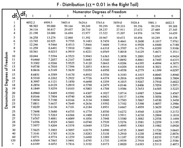
33 We can also derive the test for the general case. Consider the unrestricted model y = β 0 + β 1 x 1 + β 2 x β k x k + ε where the number of parameters in this model is k + 1 Suppose we are interested in testing q exclusion restrictions; i.e, the null that q of the variables in the equation above have coefficients equal to zero. We can state the null as So, our restricted model is H 0 : β k-q+1 = 0,, β k = 0 y = β 0 + β 1 x 1 + β 2 x β k-q x k-q + ε Remember, we want to look at the relative increase in the SSR when going from the unrestricted to the restricted model. The F statistic is defined as F ( SSRr SSRur ) / q SSR / ( n k 1) ur where SSR r is the sum of squared residuals from the restricted model and SSR ur is the sum of squared residuals from the unrestricted model

34 To use the F stat, we must know its sampling distribution under the null so we can choose critical values and form rejection rules. It can be shown that, under H 0, F is distributed as an F random variable with (q, n k 1) degrees of freedom F ~ F q, n-k-1 (see our probability theory notes for more details on the F stat) We will reject the null when F is large enough again, this will depend on our chosen significance level (see Table G.3 for critical values for the F distribution) We reject H 0 in favor of H 1 at the chosen level of significance if F > c

35

36 Back to our baseball example F = (SSR r SSR ur )/q SSR ur /(n k 1) = ( )/ /( ) = 9.55 Critical value for testing joint significance at 1% level is approximately 3.78 (see table) So, we easily reject the hypothesis that bavg, hrunsyr, and rbisyr have no effect on salary Is this outcome surprising due to the fact that none of these variables are individually statistically significant? What is happening is that the two variables hrunsyr and rbisyr are highly correlated, and this multicollinearity makes it difficult to uncover the partial effect of each variable; this is reflected in the individual t stats The F stat tests whether all three variables are jointly significant, and multicollinearity between hrunsyr and rbisyr is much less relevant for testing this hypothesis In general, the F stat is useful for testing exclusion of a group of variables when the variables in the group are highly correlated We can substitute in for SSR (= SST(1 R 2 )) and express our F-stat in terms of R 2 F = (R 2 ur R 2 r )/q (1 R 2 ur )/(n k 1) [Show t-stat in Mata. Show f-stat in canned Stata procedure]

37 F Statistic for Overall Significance of a Regression Consider the null H 0 : x 1, x 2, x k do not help explain y This says is that none of the explanatory variables share a statistically significant relationship with y This is stated in terms of the parameters of our model as H 0 : β 1 = β 2 = = β k = 0 The alternative is that at least one of the betas is different from 0 This implies the restricted model of y = β 0 + ε The F stat for testing the null is thus F = (R 2 )/k (1 R 2 )/(n k 1) here, k = q because the # of restrictions is equal to the # of variables in the population model The restricted R 2 is simply zero because all independent variables have been dropped when estimating the restricted model. If we fail to reject the null, then there is no evidence that any of the independent variables help to explain y This overall significance of the regression is generally reported in regression software (show STATA example)

38 Testing General Linear Restrictions Sometimes we might be interested, for theoretical reasons, in testing a null hypothesis that is more complicated than just excluding some independent variables Consider the following log(price) = β 0 + β 1 log(assess) + β 2 log(lotsize) + β 3 log(sqrft) + β 4 bdrms + ε where price is house price, assess is the assessed housing value before home sold, lotsize is the size of the lot in feet, sqrft is the square footage of the house, bdrms is the number of bedrooms Suppose we want to test whether the assessed housing price is a rational valuation i.e, an X% change in assess should be associated with an X% change in price i.e., β 1 = 1 In addition, the remaining covariates should not help to explain variation in price, conditional on the assessed value Thus, we have the following null H 0 : β 1 = 1, β 2 = 0, β 3 = 0, β 4 = 0

39 Unrestricted model: log(price) = β 0 + β 1 log(assess) + β 2 log(lotsize) + β 3 log(sqrft) + β 4 bdrms + ε (1) Restricted model: log(price) = β 0 + log(assess) + ε which we can rewrite as follows for estimation purposes log(price) - log(assess) = β 0 + ε (2) This is just a model with an intercept, but with a different dependent variable than in the first equation above The procedure for computing the F stat is the same Calculate the SSR r from equation (2) and the SSR ur from equation (1) One point to emphasize here We cannot use the R 2 version of the F stat because the dependent variable is different across the two equations and, thus, the total sum of squares from the two regressions will be different As a general rule, the SSR form of the F stat should be used if a different dependent variable is needed for running the restricted regression [this is easily implemented in STATA show with example]

40 back

41 -finish hypothesis testing with Wald and LR/LM tests