INVESTIGATIONS OF A PRINTED CIRCUIT HEAT EXCHANGER FOR SUPERCRITICAL CO2 AND WATER HOSEOK SONG. B.S., Inha University, South Korea, 2004 A THESIS

Transcription

1 INVESTIGATIONS OF A PRINTED CIRCUIT HEAT EXCHANGER FOR SUPERCRITICAL CO AND WATER by HOSEOK SONG B.S., Inha University, South Korea, 004 A THESIS submitted in partial fulfillment of the requirements for the degree MASTER OF SCIENCE Department of Mechanical and Nuclear Engineering College of Engineering KANSAS STATE UNIVERSITY Manhattan, Kansas 007 Approved by: Major Professor Dr. Akira T. Tokuhiro

2 Abstract In the STAR-LM (Secure Transportable Autonomous Reactor-Liquid Metal) reactor concept developed at Argonne National Laboratory (ANL), a supercritical CO (S-CO ) Brayton cycle is used as the power conversion system because it features advantages such as a higher efficiency due to less compressive work, and competitive cost due to a reduced complexity and size. From the components of the cycle, high performance of both the recuperator and precooler has a large influence on the overall cycle efficiency and plant economy. One attractive option for optimizing the performance of the cycle is to use an high efficiency heat exchanger such as the Printed Circuit Heat Exchanger (PCHE) manufactured by Heatric. The PCHE is a compact heat exchanger with high effectiveness, wide operating range, enhanced safety, and low cost. PCHEs are used in various industrial applications, but are relatively new to the nuclear industry. In this study, performance testing of a PCHE using supercritical CO and water as heat transfer media were performed at ANL. The heat transfer characteristics of the PCHE under operating conditions of the STAR_LM precooler were investigated. The S- CO, defined the hot-side, had its outlet condition near the pseudocritical point at 7.5MPa (~31-3 C). We found that of all the thermophysical properties undergoing rapid change near the critical point, heat transfer for S-CO is strongly correlated with the specific heat of CO. Additional experiments performed with different bulk temperatures and pressures on the hot side also supported this conclusion. We proposed plotting the heat transfer results, (Nu + Pr /3 ) versus (RePr 4/3 ), based on an order-of-magnitude analysis, to reveal the close proximity of the outlet to pseudocritical conditions. In order to check the experimental results, a nodal model of a segmented PCHE using a traditional log-mean temperature difference method was developed. This approach provided the temperature distribution along the heat exchanger. Additionally a CFD simulation (FLUENT) of a 4-layer, zig-zag channeled PCHE was developed. Comparison of the simulation and LMTD nodal model revealed that indeed specific heat strongly influenced the heat transfer.

3 Table of Contents List of Figures... v List of Tables... ix NOMENCLATURE... xi Acknowledgements...xiii CHAPTER 1 - Introduction Research background Objectives... 7 CHAPTER - Literature Review STAR-LM system Supercritical Fluid Micro and zigzag channels Printed Circuit Heat Exchanger CHAPTER 3 - Test Loop Printed Circuit Heat Exchanger (PCHE) Heating system Cooling system Heat sink Cooling Pump and Motor Pressurizer Flow meter Differential pressure transmitter Data acquisition System... 6 CHAPTER 4 - Estimate of the Printed Circuit Heat Exchanger Internal Configuration Zigzag angle Heat transfer area and wall thickness of metal wall Consideration of the metal wall between channels CHAPTER 5 - Pressure drop iii

4 CHAPTER 6 - Heat transfer with water and water in the PCHE CHAPTER 7 - Heat transfer with CO and water Heat transfer in the pseudocritical region Heat transfer between CO and water under STAR-LM system conditions CHAPTER 8 - Predicted temperature distribution in the PCHE Analytical calculation method Calculation results CHAPTER 9 - Conclusion References Appendix A - Experimental Data... 9 Appendix B - Error analysis Appendix C - Order of magnitude analysis Appendix D - Experimental procedure D.1. Initial charge of CO D.. Supplemental Charging of CO D.3. Experiment procedure Appendix E - Thermophysical properties of CO Appendix F - Results of the nodal calculation Appendix G - Published papers iv

5 List of Figures Figure 1.1Greenhouse Gas Emission from Electrical production []... 1 Figure 1. Comparison of electricity production costs []... Figure 1.3. Process diagram for the STAR-LM reactor [0]... 3 Figure 1.4 Specific heat of CO at 7.4 MPa... 4 Figure 1.5 Density profile at 7.4 MPa... 4 Figure 1.6 Minimum temperature optimization [0]... 5 Figure.1 P-T diagram of CO... 9 Figure 3.1 -D picture of the experimental loop Figure 3. 3-D picture of the experimental loop Figure 3.3 Comparison a PCHE with a shell and tube heat exchanger [5] Figure 3.4 The details of a PCHE [5] Figure 3.5 The picture of the PCHE Figure 3.6 The power supply and the copper bus bars Figure 3.7 The water controller and water lines... 0 Figure 3.8 The tube-in-tube heat exchanger... 1 Figure 3.9 GCI Icewagon chiller... 1 Figure 3.10 The magnetic gear pump and the TEFC motor... Figure 3.11 Pressurizer... 3 Figure 3.1 CO flow meter... 4 Figure 3.13 Water flow meter... 4 Figure 3.14 Rosemount Model 088 and 3051 pressure transmitter... 5 Figure 3.15 Data acquisition system and control panel... 6 Figure 4.1 The cross section shape of the channel... 9 Figure 4. Microchannel structure of a PCHE Figure 4.3 Simplified longitudinal channel shape Figure 4.4 (a). The simplified cold channel of the PCHE... 3 Figure 4.5 (b). The same size matrix with the simplified PCHE... 3 v

6 Figure 4.6 Simplified longitudinal channel shape of cold side Figure 4.7 Sectional area of TiTech s PCHE [8] Figure 4.8 Ratio of the thermal resistance of the metal wall to the total resistance Figure 5.1 Moody friction factor with water on the hot and cold sides... 5 Figure 5. Fanning friction factor with CO on the hot side Figure 6.1 Simplified heat exchanger figure Figure 6. The correlation between heat transfer coefficient and Reynolds number for CO [8] Figure 6.3 Average heat transfer coefficient for water Figure 7.1 Specific heat and density of CO at 7.5MPa Figure 7. Viscosity and thermal conductivity of CO at 7.5MPa Figure 7.3 Heat transfer coefficient versus bulk temperature from Liao s paper[14]... 6 Figure 7.4 Nusselt number versus bulk temperature from Liao s paper [14]... 6 Figure 7.5(a) Liao s result at 8.0MPa with CO Figure 7. 5(b) Liao s result at 10MPa with CO Figure 7. 6(a) The heat transfer coefficient versus the temperature at 7.5MPa [6] Figure 7. 6(b) The heat transfer coefficient versus the temperature at 8.0MPa [6] Figure 7. 6(c) The heat transfer coefficient versus the temperature at 8.5MPa [6] Figure 7. 7 Average heat transfer coefficient versus the bulk temperature Figure 7. 8 The precooler operating range in the STAR-LM system Figure 7. 9 The PCHE operating range Figure 7.10 The specific heat versus temperature normal to the pseudocritical point Figure 7.11 Heat transfer coefficient with Reynolds number of Test A and B Figure 7.1 The heat transfer coefficient with the temperature of Huai et al. [6]... 7 Figure 7.13 The heat transfer coefficient with CO of Test A, B, and C Figure 7.14 The result of the order of magnitude method Figure 8.1 A simplified drawing of the PCHE Figure 8. A section of the simplified drawing of the PCHE Figure 8.3 The comparison of results of the 15 and 0 piece model Figure 8.4 The temperature distribution of Test A Figure 8.5 Thermal diffusivity of CO at 7.5MPa vi

7 Figure 8.6 The calculation results from the nodal calculation and CFD Figure E.1 Specific heat at 74bar Figure E. Density at 74bar Figure E.3. Thermal Conductivity at 74bar Figure E.4 Enthalpy at 74bar Figure E.5. Viscosity at 74bar Figure E.6. Thermal diffusivity at 74bar Figure E.7. Specific heat at 75bar Figure E.8. Density at 75bar Figure E.9. Enthalpy at 75bar Figure E.10. Thermal conductivity at 75bar Figure E.11. Viscosity at 75bar Figure E.1. Thermal diffusivity at 75bar Figure E.13. Specific heat at 80bar... 1 Figure E.14. Density at 80bar... 1 Figure E.15. Thermal conductivity at 80bar Figure E.16. Viscosity at 80bar Figure E.17. Enthalpy at 80bar Figure E.18. Thermal diffusivity at 80bar Figure E.19. Specific heat at 85bar Figure E.0. Density at 85bar Figure E.1. Thermal conductivity at 85bar Figure E.. Enthalpy at 85bar Figure E.3. Viscosity at 85bar Figure E.4. Thermal diffusivity at 85bar Figure E.5. Specific heat at 90bar Figure E.6. Density at 90bar Figure E.7. Enthalpy at 90bar Figure E.8. Thermal conductivity at 90bar Figure E.9. Viscosity at 90bar Figure E.30. Thermal diffusivity at 90bar vii

8 Figure F.1. Temperature distribution of Test A Figure F.. Temperature distribution of Test A Figure F.3. The temperature distribution of Test A Figure F.4. The temperature distribution of Test A Figure F.5. The temperature distribution of Test B Figure F.6. The temperature distribution of Test B Figure F.7. The temperature distribution of Test B Figure F.8. The temperature distribution of Test B Figure F.9. The temperature distribution of Test B Figure F.10. The temperature distribution of Test C Figure F.11.The temperature distribution of Test C Figure F.1. The temperature distribution of Test C Figure F.13. The temperature distribution of Test C Figure F.14. The temperature distribution of Test C viii

9 List of Tables Table 1.1. Cycle efficiency according to the outlet temperature of the precooler [0]... 6 Table 3.1 Design specifications for PCHE Table 3. Pressure transmitters... 5 Table 4.1 Design specifications for PCHE from Heatric... 7 Table 4. Test results provide by Heatric... 8 Table 4.3 Geometry and configuration of TiTech s PCHE [8] Table 4.4 Reynolds number provide by Heatric Table 4.5 Convection heat transfer coefficient provide by Heatric... 4 Table 4.6 Dimension of the PCHE Table 4.7 The properties of Stainless Steel Table 4.8 The specification of TiTech s heat exchanger [8] Table 4.9 A test condition of CO /water Table 7.1 The error propagation on the CO by the water heat transfer coefficient Table A.1 Experiment range of pressure drop on the hot side... 9 Table A. Experiment range of pressure drop on the cold side Table A.3 Experiment range of water to water test Table A.4 The test conditions of Test A Table A.5. The test conditions of Test B Table A.6 The test conditions of Test C Table B.1 Rule of error analysis Table B. Experimental data Table B.3 Enthalpy for the hot side Table B.4 Density and viscosity for CO Table E.1 Thermal properties at 74bar Table E.. Thermophysical properties of CO at 75bar Table E.3 Thermophysical properties at 80bar Table E.4. Thermophysical properties at 85bar ix

10 Table E.5. Thermophysical properties at 90bar x

11 NOMENCLATURE Symbols Description A area, m A c cross-sectional area, m C f friction coefficient c p specific heat at constant pressure, J/kg K D diameter, m D h hydraulic diameter, m f friction factor G mass velocity, kg/m s Gr Grashof number h convection heat transfer coefficient, W/m i enthalpy, J/g j H Colburn j factor for heat transfer k thermal conductivity, W/m K L metal wall thickness, m m mass flow rate, kg/s Nu Nusselt number P perimeter, m p pressure, N/m Pr Prandtl number Q volumetric flow rate, gpm or m 3 /s q heat transfer rate, W R t thermal resistance, K/W Re Reynolds number r radius, m S supercritical fluid xi

12 St Stanton number T temperature, K U overall heat transfer coefficient, W/m K u, v, w mass average fluid velocity components, m/s V volume, m 3 ; fluid velocity, m/s Greek Letters α Thermal diffusivity, m /s p pressure drop, N/m T lm μ log mean temperature difference viscosity, Kg/s m ν kinematic viscosity, m /s ρ mass density, kg/m 3 τ shear stress, N/m Subscripts ANL Argonne National Laboratory b, bulk bulk fluid c cross-sectional; cold side CO carbon dioxide D diameter h hydrodynamic; hot side H O water in inlet out outlet t thermal total total w, wall wall xii

13 Acknowledgements I would like to thank Dr. Akira Tokuhiro for his guidance and for the opportunity to study at Kansas State University. I would also like to thank Dr. Dae H. Cho and Steve Lomperski for helping me on the experiment at Argonne National Laboratory. I would also like to express my thanks to the members of my committee for devoting their time so that this project could be successfully completed. I would like to thank to my family and J. H. Yoo for their support. xiii

14 CHAPTER 1 - Introduction 1.1 Research background The world s population is predicted to increase up to about 10 billion by 050. As the world population is increasing, the consumption of energy is also growing. So the shortage of energy has become a major issue these days due to the rapid growth of population. In considering global electricity consumption, the International Energy Agency projects a doubling of world electricity demand by 030, creating the need for 740GWe of new generating capacity in the next quarter century. In 005 the global generating capacity is 367GWe. The reasons why nuclear power is mainly considered are due to its environmental and economic competition. First, nuclear energy is promising as shown in Figure 1.1. If coal power plant is replaced with nuclear power plant, every tonnes of uranium used for electricity would save the emission of about one million tonnes of carbon dioxide, relative to coal []. Figure 1.1Greenhouse Gas Emission from Electrical production [] 1

15 Secondly, nuclear energy is competitive in generating costs compared with other energy sources. As Figure 1. shows, a nuclear power plant provides electricity at the most competitive price. Figure 1. Comparison of electricity production costs [] The electricity production cost with each energy source is evaluated based on fuel cost, operation cost and maintenance cost. As shown in Figure 1., the gas production cost is 4 times more than that of nuclear. However, nuclear plants have relatively high capital costs. The competitiveness of nuclear energy depends on the capital cost of the plant, and reduction of capital can be expected by reduced construction time. For this reason, the Secure Transportable Autonomic Reactor (STAR) was designed by Argonne National Laboratory (ANL) to meet the goals of economics, proliferation resistance, sustainability, and the possibility of long-term operation (15-0 years) without refueling [0]. The STAR-LM system employs closed cycle gas turbines because compared to a steam cycle, the closed cycle gas turbines are simple, compact, and less expensive, and have shorter construction periods, thus reducing the capital costs [0].

16 The STAR-LM cycle uses lead (Pb) as reactor coolant and the supercritical CO (S-CO ) as the working fluid. As Figure 1.3 shows, the STAR-LM cycle consists of STAR reactor, turbine, high temperature recuperator, low temperature recuperator, precooler, and compressors. CO has unique characteristics near its critical point. Figure 1.4 and Figure 1.5 show the density and specific heat with critical point and the outlet temperature of the precooler in the STAR-LM system CO Kg/s 439 TURBINE 7.46 HTR Pb atm RHX Eff = 44.9 % T,C T,C COMP. # AIR Q,MWP,MPa 7.46 RVACS CORE AVG Temperature, o C HOT 400 FUEL CLADDING Pb LTR CORE OUT COMP. # MID Pressure, MPa Precooler 1845 Kg/s IN COOLER % REACTOR VESSEL Tcl Tfo Tci Tco Tc 35% Figure 1.3. Process diagram for the STAR-LM reactor [0] 3

17 Precooler outlet 74 bar c p (J/g*K) Critical Temperature temperature Temperature( o C) Figure 1.4 Specific heat of CO at 7.4 MPa bar 500 ρ(kg/m 3 ) Critical Temperature Precooler outlet temperature Temperature( o C) Figure 1.5 Density profile at 7.4 MPa 4

18 The critical temperature is o C. The precooler outlet temperature is 31.5 o C in the STAR-LM system. The specific heat reaches a maximum value at the supercritical point as shown in Figure 1.4. We thus can realize high efficiency if we operate the heat exchanger in this thermophysical regime. The density decreases near the critical temperature as shown in Figure 1.5. This characteristic reduces the required compressor work done on CO as it is compressed just before the density decreases rapidly near the critical point in the compressor. Figure 1.6 Minimum temperature optimization [0] Figure 1.6 shows the cycle efficiency versus minimum temperature in the STAR- LM system. The minimum temperature is the outlet temperature of the precooler in the STAR-LM system. The highest efficiency is achieved at the critical point as shown. However, the STAR-LM system has a slightly higher temperature on the outlet of the precooler. It is 31.5 o C. With this temperature, the calculated system efficiency is 43.8% [0]. There are several reasons to have a higher temperature than the critical temperature (30.98 o C). If the precooler outlet temperature is 31 o C, the length of the 5

19 precooler is estimated as 6.5m [0] as shown in Table 1. As the outlet temperature of the precooler increases slightly to 31.5 o C, the length of the precooler decreases down to 1.1m [0]. Thus, although an increase in outlet temperature requires more compressor work, the relative decrease in length is more than 50% relative to 6.5m. Additionally, for compressor durability, it is necessary to avoid two phase flow in the compressor [0] o C is too close to the critical point, o C. In order to keep CO in a supercritical state, one must have a margin of safety; 31.5 o C was deemed practical and achievable. For the reasons discussed above, the outlet temperature of the precooler is set slightly higher than the critical point. Table 1.1. Cycle efficiency according to the outlet temperature of the precooler [0] Precooler outlet temp o C 31.5 o C Heat exchanger length 6.5m 1.1m Compressor #1 work 7.6MW 40.0MW Cycle efficiency 45.8% 43.8% In this study, we focus on the PCHE as the precooler of the STAR-LM system due to its importance as discussed above based on the operating condition as shown in Figure 1.3. In addition, more experiments are conducted with changing the temperature and pressure with supercritical CO. 6

20 1. Objectives The present work reports on the performance of a Printed Circuit Heat Exchanger (PCHE) as a key component in the power conversion system of a Generation IV advanced nuclear system (STAR-LM). The PCHE is being considered as a precooler and the recuperators () in the STAR-LM system. The Heatric PCHE of a proprietary design was performance tested at Argonne National Laboratory using water and supercritical CO as heat transfer media. We followed the following objectives based on the scope-of-work agreed upon with support from DOE. First, the PCHE heat transfer lengths were verified based on limited information provided by Heatric. As complete, detailed specifications were not provided, we estimated the basic dimensions of the PCHE such as zigzag channel angle and channel diameter. From this, we estimated the size of the interior hot and cold channels. Second, the flow characteristics of the PCHE were investigated experimentally. From this, the hydraulic characteristics, similarities and differences, of both the hot and cold side were noted. Third, heat transfer characteristics of the PCHE with water on both the hot and cold sides were studied experimentally. The convective heat transfer coefficient with water was determined. These measurements were carried out prior to measurement of the heat transfer coefficients with CO. Fourth, heat transfer characteristics of the PCHE with CO were investigated experimentally. This was the primary goal of this study. Operating experience with the CO loop, near the critical point, was also gained. Fifth, analytical methods to predict and verify the experimental results were developed. In particular, we sought to estimate the temperature distribution in the PCHE. The analysis was based on the measured overall heat transfer coefficient in CO /water test, the thermophysical properties of CO (about the critical point) and water, and a modified heat exchanger analysis. Finally, a simplified computational fluid dynamics model of the PCHE was developed to further support our analytical approach. 7

21 CHAPTER - Literature Review.1. STAR-LM system The Generation IV Advanced Reactor systems are expected to achieve significant reductions in capital and operating costs by taking advantage of the benefits of modular construction, up-to-date manufacturing practices, design simplifications, design innovations, and advanced technologies. Significant realistic reductions in plant costs, size, and complexity combined with a significant increase in plant efficiency may potentially be realized through the use of an advanced power conversion technology consisting of a gas turbine Brayton cycle utilizing S-CO as the working fluid. S-CO has significantly higher density (relative to helium), which reduces the need for compressive work in the bottom part of a Brayton cycle; thus increasing the overall cycle efficiency. S-CO Brayton cycle has been considered as the power conversion system for the Secure Transportable Autonomous Reactor (STAR) project at Argonne National Laboratory. The STAR-LM (Liquid Metal) version is a high temperature, fast flux reactor driven by natural circulation. It employs molten lead (or lead-bismuth eutectic) as the primary coolant and uses an indirect Brayton cycle for the generation of electricity. The plant is designed to operate with a turbine inlet temperature of 550 o C and is expected to have a cycle efficiency of about 45 percent. [3] One of the key components for the S-CO power system is the regenerative heat exchanger, known as the recuperator. This is where heat exchange between two flowing streams of S-CO takes place. While the benefits of the S-CO Brayton cycle are attributed to the unique thermophysical properties of S-CO (e.g. density and specific heat), these same properties also present technical challenges to the recuperator design. The high and low temperature recuperators, HTR and LTR, respectively, each operate with S-CO on both sides of the heat exchanger. The precooler, on the other hand, uses S-CO on the hot side and H O from the ultimate heat sink on the cold side. In particular, cycle efficiency is sensitive to the effectiveness of both the recuperators and 8

22 precooler [0]. The hydraulic characteristics of the heat exchangers are also of interest because pressure drops must be considered in the task of detailed cycle optimization [8]. As S-CO is a working fluid in the STAR-LM system, past studies on supercritical fluids have been studied. In the next section, supercritical fluids such as S- CO and water will be discussed... Supercritical Fluid The critical point of a fluid is defined as a point where the difference between the vapor and liquid disappears [11]. The region above the critical point is called a supercritical phase as shown in Figure.1. The upper right region defines the supercritical state. The critical point of CO is at o C and 7.38MPa. 9 Supercritical fluid pseudo-critical line Pressure ( MPa ) 7 6 Liquid Gas Critical Point o C 7.38 MPa Pressure ( psi ) Temperature ( o C ) 580 Figure.1 P-T diagram of CO 9

23 In supercritical phase, the fluid cannot be defined to be in a liquid state or gas state. In supercritical region, the pseudocritical temperature is the most interesting factor because thermophysical properties change dramatically. In the optimization of the STAR- LM system by Moisseytsev, these properties were considered to achieve the highest efficiency. For each supercritical pressure, the value of temperature at which the specific heat capacity reaches a peak value is called the pseudocritical temperature. Supercritical fluids have unique changes in thermoproperties near the pseudocritical temperature. When bulk temperature decreases below the pseudocritical temperature, the supercritical fluid changes from a gas-like state to a liquid-like state. As such, heat transfer studies in the supercritical region have been carried out, both experimentally and theoretically by a number of investigators. Although there are a number of heat transfer studies with pure substances and refrigerants, we will primarily concentrate on CO unless other fluids contribute to the purpose of this work. Sabersky et al. [30] investigated forced convection heat transfer of CO at near the critical point with an electrically heated flat plate. They showed that the forced convection heat transfer coefficient of CO near the critical point became large as the fluid temperature approached the pseudocritical point. Huai [6], J. Pettersen [8], and Wood et al. [34] showed that for horizontal convection flow, the heat transfer also changes with specific heat change. In other words, the heat transfer begins increasing below the pseudocritical point; reaches a peak value at, and then decreases beyond the pseudocritical point at the given pressure as the temperature increases. A number of correlations for heat transfer of supercritical fluids have been established theoretically and experimentally. Bringer et al. [3] proposed a correlation for supercritical water up to 34.5MPa and also for a CO : 0.77 Nu x = C Re Prw where subscript w means wall, C=0.066 for water and C= for CO McAdams [19] proposed use of the much quoted Dittus and Boelter equation for forced convective heat transfer in turbulent flows and at supercritical pressures: 10

24 Nu b = Reb Prb where subscript b means bulk. Swenson et al. [33] studied heat transfer to supercritical water in smooth-bore tubes. They showed that the conventional correlations did not work well because of rapid changes in themophysical properties of supercritical water near the pseudocritical point. Liao et al. [14, 15] investigated heat transfer from S-CO in horizontal micro circular tubes cooled to a constant temperature. Stainless steel tubes having diameters of 0.70, 1.40, and.16mm were used at pressures from 74 to 10bar, temperatures from 0 o C to 110 o C, and mass flow rates from m = 0.0 to 0.kg/min, and Reynolds numbers from Re=10 4 to They presented a correlation for horizontal flow for the circular tubes of d=0.70, 1.40, and.16mm as follows. Nu b = 0.14 Re 0.8 b Pr 0.4 b Gr Re b 0.03 ρ w ρb 0.84 c c p p, b The maximum relative error between the above correlation and the experimental data is about 1.8%. The experiment result shows that the previous conventional correlation for normal size tubes cannot predict the heat transfer coefficient in microchannels. Pettersen et al. [9] investigated heat transfer and pressure drop characteristics of S-CO in 0.79 mm microchannel tubes at pressures of 81, 91, and 101bar under cooling conditions. The results showed that the closer temperature is to the pseudocritical point, the higher the peak heat transfer coefficient. The heat transfer coefficient changed along with specific heat at each pressure. The heat transfer coefficient increases as the pressure approaches the critical pressure of CO (73.8bar). 11

25 .3. Micro and zigzag channels Plate heat exchangers with wavy or zigzag channels provide excellent heat transfer performance as evaporators and condensers in small refrigeration system [13]. For compactness, a printed circuit heat exchanger also employs zigzag microchannels where the hydraulic channel sizes between 0.1 mm and mm are defined as microchannels [10]. Zigzag microchannels elongate the heat exchange length within heat exchangers to facilitate heat transfer. Past investigations have shown different trends in heat transfer and flow regimes between traditional and microchannel based heat exchangers. For example, Peng, X. F. et al. [5] studied flow characteristics in a rectangular microchannel with the hydraulic diameters of D h = 0.133~0.367 mm. They found that the transition from laminar flow occurs at about Re=300 and the transition to the fully turbulent flow regime at about Re=1000. They showed that the heat transfer and flow characteristics were affected by the geometric parameters experimentally. They found that there was an optimum channel size when the width to height ratio is 1/ or. Wang and Peng et al. [7] studied forced convection of water and methanol in rectangular channels. They claimed that the heat transfer could be predicted by a modification of the Dittus-Boelter equation by modifying the experimental constant from 0.03 to : Nu = Re 4 / 5 Pr 1/ 3 In their experiment, liquid temperature, velocity and microchannel size changed the transition and laminar heat transfer behavior in microchannels. It was shown that at a given liquid temperature and velocity, transition to turbulent heat transfer occurs at lower Re, as the channel size becomes smaller. The transition is initiated at about Re=1000~1500, which is small compared with the conventional size channels. Similar experiments using microchannels were conducted by Adams et al [1]. They investigated single-phase forced convection in circular microchannels with diameters, D= 0.76 and D=1.09 mm. They calculated heat transfer coefficients and Nusselt numbers for water. The results were compared with predicted values calculated using a correlation for traditional channels. The correlation is the following: 1

26 ( f / 8)(Re 1000) Pr Nu = 1/ / 3 K + 1.7( f / 8) (Pr 1) where K = (900 / Re) [ 0.63/( Pr) ],and f = (1.8 log(re) 1.64). Adam s experimental results were larger than the predicted values because the Gnielinski s correlation could not explain the enhancement in heat transfer by the decrease of the microchannel size. They showed that enhancement in heat transfer increased as the channel diameter decreased. Peiyi et al. [4] investigated the flow friction and heat transfer of gases flowing through microchannels and observed that the convective flow heat transfer characteristics departed from conventional channels. They showed that the friction factors were above those obtained from the traditional Moody chart and that the transition from laminar to turbulent flow occurred much earlier, at Reynolds numbers of about 400~900 due to the roughness of channels. The published literatures also contain several studies on zigzag channels and wavy channels. These channel configurations have been used for compactness and to generally increase the heat transfer path length. O Brien et al. [3] investigated forced convection heat transfer coefficients and friction factors for flow in a corrugated duct with corrugation angle of 30 degrees, width of 5.08 cm, and height of cm. The Reynolds number ranged from 1500 to They showed, through flow visualization, a highly complex flow pattern including a strong forward flow and recirculating flow. Their study showed heat transfer enhancement with the corrugated duct flow relative to a conventional parallel-plate heat exchanger. Y. S. Lee et al. [13] studied heat transfer in wavy channels. They showed that the laminar and the turbulent flow regimes in the corrugated channels are not distinguished as in circular pipes. That is, laminar flow for a circular straight channel may not be laminar in a wavy channel. In fact, they showed that the heat transfer does not change in both laminar and turbulent regimes for channel width less than 30 mm, while the distinction is more apparent in wider channels. Jiao et al. [9] studied the flow resistance and heat transfer in a zigzag duct. They showed that the critical Reynolds number laminar flow to turbulent flow transition is 13

27 about 100 to 150. Also, heat transfer experiments for various zigzag ducts and plate heat exchangers evidently revealed no generalized dimensionless correlation for zigzag channels. They proposed correlations based on experimentally measured Reynolds and Prandtl numbers..4. Printed Circuit Heat Exchanger One type of compact heat exchanger that is under consideration to serve as a recuperator and precooler is a PCHE [17]. A PCHE consists of stacked plates with each plate chemically-etched with microchannels; the plates are then diffusion bonded. In fact, Moisseytsev [0] showed a comparison of 9 heat exchanger designs for the STAR-LM LFR concept: 1) stacked U-tubes heat exchanger, ) U-tubes heat exchanger, 3) concentric tubes heat exchanger, 4) straight tubes heat exchanger, 5) straight annuli heat exchanger, 6) helical coil heat exchanger, 7) plate type heat exchanger with U-turn, 8) counter flow plate type heat exchanger, and 9) printed circuit heat exchanger. A compact heat exchanger design such as a PCHE was indeed much smaller than traditional heat exchanger types. However, basic heat transfer data to evaluate the PCHE s performance, under reactor-relevant conditions, are lacking. Further its performance level in an actual power plant is uncertain. The only other published work using the PCHE with S-CO are works by Ishizuka et al. [8]. Their PCHE unit was rated at 3kW as compared to our 17.5kW. Ishizuka et al. [8] conducted thermal hydraulic tests with a 3kW Heatric heat exchanger using CO. The hot and cold side pressures ranged between ~4MPa (0~40bar) and 6~11MPa (60~110bar), respectively, with fluid temperatures between 110 o C and 80 o C. The CO on the cold side was in many cases supercritical (critical point at 7.38MPa, o C) though all tests were carried out far from the pseudocritical region where there are sharp changes in fluid properties with temperature. The effectiveness (η) of the heat exchanger was found to be very high, 99%, for all test cases. Pressure loss and heat transfer coefficients correlated well with Reynolds number and there were no notable differences between subcritical and supercritical conditions. The average heat transfer coefficient increased with the CO pressure. 14

28 CHAPTER 3 - Test Loop Figure 3.1 and 3. are schematics of the present experimental loop. The loop is located at ANL. The test apparatus consists of a closed CO loop and a water line in an open loop. The CO loop consists of a pump, a flow meter, an electrically heated pipe section (1m), two pressure meters, the Printed Circuit Heat Exchanger rated at 17.5kW, a pressurizer, 9 K-type thermocouples, two platinum RTDs (Resistance Temperature Detectors) an accuracy of ±0.1 o C, a CO reservoir tank, a helium reservoir tank. For this study, the helium reservoir tank was not used. The water line consists of a flow meter, pressure meter, and two platinum RTDs. HOT LEG TF P HEATRIC HX TF COLD LEG FILTER Water side TF P TF P CO side FILTER HOT LEG P P = ABSOLUTE PRESSURE = DIFFERENTIAL PRESSURE TF = FLUID TEMPERATURE TW = WALL TEMPERATURE = RELIEF VALVE COLD LEG CORIOLIS FLOWMETER CO LEVEL DETECTOR P EXHAUST GEAR PUMP CO PRESSURIZER T T F TW W TW TW TF DIELECTRIC UNION TF TF TF 0-60 VAC 5000 A POWER SUPPLY 440 VAC, 770 A Figure 3.1 -D picture of the experimental loop 15

29 Power supplier PCHE Water line Bus bar Pump CO line Heated pipe section Figure 3. 3-D picture of the experimental loop 3.1. Printed Circuit Heat Exchanger (PCHE) The Printed circuit heat exchanger (PCHE) is a compact heat exchanger manufactured by Heatric. In comparing the PCHE against conventional heat exchangers of the same duty, the PCHE is up to 85 % smaller than the equivalent shell and tube heat exchanger [5] as shown in Figure 3.3. Shell & tube heat exchanger PCHE Figure 3.3 Comparison a PCHE with a shell and tube heat exchanger [5] 16

30 The heat exchange path is created by chemically etching the flow path on metal sheets (Stainless steel 316) as shown in Figure 3.4(a). The plates are joined one by one through the method of diffusion bonding as shown in Figure 3.4(b). The diffusion bonding process forms bonds at the molecular level under high pressure and temperature. The diffusion bonding generates continuity between sheets so that contact resistance is eliminated and thus effective heat transfer promoted. Figure 3.4(c) shows the grain growth between surfaces of etched plates. (a) Etched plate (b) Stacked plates (c) Micrograph of a PCHE Figure 3.4 The details of a PCHE [5] The PCHE for this study is rated for a maximum pressure of 1.6MPa for the hot channel and 8.3MPa for the cold channel. The unit measures mm, weights 03kg, and has a heat exchange capacity of 17.5kW. Figure 3.5 shows a top down view of the unit. This compact heat exchanger is designed for the test between high and low pressure streams of S-CO, but in order to benchmark its performance, the PCHE was tested here with water and S-CO as the heat transfer media. Additional details of PCHE 17

31 are provided in Table 3.1. The unit has the same hydraulic diameter, 0.9mm, volumetric capacity, liters, and heat transfer area, 5.6m on both the hot and cold sides as quoted in Table 3.1. Hot side inlet Cold side inlet Cold side outlet Hot side outlet Figure 3.5 The picture of the PCHE Table 3.1 Design specifications for PCHE Hot side Cold side Design pressure (bar) Design temperature ( o C) Flow area (mm ) Number of channels Hydraulic diameter (mm) Capacity (liters) Total heat transfer area (m ) 5.6 Total mass (kg) 03 Dimensions (mm) 10 x 00 x

32 3.. Heating system The CO in the primary loop is heated via electrical resistance heating by direct current through the one meter section of the horizontal pipe as shown in Figure 3.1 and 3.. Figure 3.6 shows the power supply and copper bus bar. The copper bus bars provide the electrical connection between the power supply and the pipe section. The capacity of the power supply is 300kW. The CO is heated as it flows through the pipe section. The electrical resistance has a maximum temperature limit of 538 o C. To protect the experimental loop, this loop automatically shuts down when the wall temperature inside the pipe section exceeds 538 o C. The temperature of the pipe section can be controlled by controlling the power output of the power supply. Power supply Copper bus bar Figure 3.6 The power supply and the copper bus bars 3.3. Cooling system Heat sink When the experiment is conducted, water is the working fluid on the cold side and exchanges heat with the hot side. The water is supplied from a water tank located in the basement of the experimental room. The maximum flow rate of the water is 4gpm (0.5 19

33 L/sec). Two valves are connected with the hot water line and the cold water line as shown in Figure 3.7. The temperature of the water through the loop can be controlled by adjusting the valves that vary the volumetric flow rate of hot and cold water in the supply. Also, cold water is provided to cool the power supply. The used water is dumped through a drain. Figure 3.7 shows a picture of the water valves and drain line. Cold water line Hot water valve Hot water line Water drain Cold water valve Figure 3.7 The water controller and water lines 3... Cooling Prior to the experiment, the CO line was first filled into the intended loop from the CO reservoir tank. If the CO loop pressure on filling did not reach the targeted pressure, we need to increase the loop pressure. The experimental loop as built does not have a booster pump, so we had to improvise a way to reach the targeted pressure of the CO loop. In order to charge the loop to higher pressure, we cool the CO loop. As the CO cools, the pressure of the CO decreases correspondingly. Subsequently, as the loop attains a lower pressure, we can add more CO just using the CO reservoir tank. 0

34 In order to cool down CO, water was used as a coolant. The temperature of water from the water tank was about 0 o C. It was not cold enough to cool down the CO. So, using a tube in the tube heat exchanger manufactured by Parker Hannifin as shown in Figure 3.8, water from the water line was cooled down by a coolant (ethylene glycol) from a chiller (a GCI Icewagon chiller). Then, the cooled water flowed into the PCHE to cool CO as described above. Tube in Tube heat exchanger Figure 3.8 The tube-in-tube heat exchanger A GCI Icewagon chiller (Model DE8AC by GCI Refrigeration Technology, Inc.) was used. This chiller had a 5 kw cooling capacity rating at 10% solution of ethylene glycol in water. Figure 3.9 shows the chiller. Figure 3.9 GCI Icewagon chiller 1

35 3.4. Pump and Motor A magnetic drive gear pump (Micropump model 10K pump) circulates the CO through the CO loop. The pump is made out of stainless steel 316 with PPS (Ryton) gears, carbon bearings, and PTFE O-ring, close coupled to a 3/4 horsepower TEFC (Totally Enclosed, Fan Cooled) motor. The motor speed is controlled by a variable frequency drive. Figure 3.10 shows the magnetic drive gear pump and the 3/4 horse power TEFC motor. The pump was installed between the flow meter and the inlet of the electrically heated pipe section on the hot side. Inlet 3/4 HP pump Outlet Magnetic gear pump Figure 3.10 The magnetic gear pump and the TEFC motor 3.5. Pressurizer We found early through trial experimental runs that the loop with S-CO was very sensitive to small changes in parameters such as temperature and pressure. The pressurizer shown in Figure 3.11 accommodates thermal expansion of CO as it is heated from room temperature to the critical point and beyond. The pressurizer dampens CO pressure fluctuations that might occur. The pressurizer is constructed from 3, schedule

36 40 pipe and is fitted with a level sensor. The CO level within the pressurizer is measured by a Mercap capacitance sensor manufactured by Milltronics Process Inc. It measures the sensor capacitance relative to that of a reference electrode. The measurement range is 0-500mm Hg with an accuracy of 0.1% of the measured value and a temperature rating up to 00 o C. Figure 3.11 Pressurizer 3.6. Flow meter A PROline Promass 80M Coriolis mass flow meter manufactured by Endress- Hauser was used to measure the mass flow of CO on the hot side. The flow meter has an accuracy of ±0.50%. This flow meter was operated independently of the physical fluid properties, such as viscosity and density. Its maximum temperature limit was 350 o C, and pressure limit, 350bar. The flow meter was installed after the heat exchanger and before the gear pump because the focus of the test was the state of the CO after the compact heat exchanger as shown in Figure 3.1. For this reason, the Coriolis flow meter was used to measure the mass flow of CO. 3

37 PROline Promass 80 M flow meter Heated pipe section Magnetic gear pump Figure 3.1 CO flow meter On the water side, a paddlewheel flow meter (OMEGA FP7001A) was installed just before the three way valve. The flow meter measured the inlet water flow rate. A picture of the flow meter is shown in Figure The flow meter had an accuracy of ±%. Water flow meter Figure 3.13 Water flow meter 4

38 3.7. Differential pressure transmitter Absolute and differential pressures were measured using a Rosemount Model 088 and 3051CD pressure transmitters manufactured by Rosemount Inc. In this experiment, we judged the stead state of experimentation based on the absolute pressure. We defined that if CO pressure fluctuate within 0.01bar, experimental data can be in steady state. Differential pressures were measured on both hot and cold sides with 3051 CD pressure transmitters. The absolute pressure within the loop and pressurizer was measured with 088 pressure transmitter. The additional specifications of pressure transmitters are given in Table 3.. Table 3. Pressure transmitters Model Accuracy % % Weight.44 lb (1.11 kg) 6.0 lb (.7 kg) Dimension 3.9 x 5.0 x 5.4 in (99 x 17 x 137 mm) 6.4 x 3. x 7.8 in. (163 x 81 x 198 mm) Figure 3.14 Rosemount Model 088 and 3051 pressure transmitter 5

39 3.8. Data acquisition System All data acquisition and process control tasks are managed by a PC executing LabVIEW 6.i under Windows 000. Sensors are connected to HP Model E1345A 16- channel multiplexer and the signals are digitized by an HP Model E136B 5 1/ digit multimeter. Figure 3.15 shows the data acquisition system and control panel. In the control panel, temperature is observed and controlled. Data acquisition system Monitors Control panel and gages PC Figure 3.15 Data acquisition system and control panel 6

40 CHAPTER 4 - Estimate of the Printed Circuit Heat Exchanger Internal Configuration 4.1. Zigzag angle One of the primary objectives of this study was to measure the heat transfer coefficient of S-CO in the prototype PCHE at ANL. To study the PCHE, the specifications of the PCHE were verified first. In fact, under the contract with Heatric, the detailed design of the heat exchanger was proprietary information and thus the heat exchanger could not be opened and inspected. Without all of the detailed heat exchanger dimensions, analyses of experimental data were not possible. However, Heatric provided a partial list of specifications. Table 4.1 shows the selected overall dimensions of the PCHE provided by Heatric. Table 4. subsequently depicts additional specifications provided by Heatric. Table 4.1 Design specifications for PCHE from Heatric Hot side Cold side Design pressure (bar) Design temperature ( o C) Flow area (mm ) Number of channels Hydraulic diameter (mm) Capacity (liters) Total heat transfer area (m ) 5.6 Total mass (kg) 03 Dimensions (mm) 10 x 00 x 100 7

41 Table 4. Test results provide by Heatric Since details such as heat transfer length (path), zigzag angle and related parameters were not provided, we had to first check these parameters associated with the flow zigzag flow configuration of the PCHE using Table 4.1 and Table 4.. First, we calculated the diameter of the hot side channel using the hydraulic diameter (D h = 0.9mm), defined as follows [6], 4 Ac Dh = = 0. 9mm (1) P In Equation 1, A c is the cross-sectional area of the channel, P is the perimeter of the channel, and D h is the hydraulic diameter. 8

42 Considering that the cross sectional shape of the channel was semicircular as seen in Figure 4.1, the diameter of the channel can be calculated using the hydraulic diameter as shown below. D r = Figure 4.1 The cross section shape of the channel Using the equation for hydraulic diameter and Figure 4.1, the diameter, D, of the channel is calculated as mm. Using the diameter, the free flow area of the hot side can be estimated using Equation. Flow area = No. of channels Area of one channel 1 π (1.5057mm) = = 1047mm () The calculated free flow area is same as that specified in Table 4.1. With the calculated diameter mm, and the channel length, the zigzag angle can be estimated. First, the length of the hot side channel can be calculated using Equation 3. Volume of channels= Lengthof channel Flow Area of channels (3) Rearranging Equation 3 yields Equation 4, which can be used to solve for the length of the hot side channel. The volume of the channels is taken from Table

43 Volume of channels Travel length = Flow Area of channels liters = 1047mm = 1.91 m (4) The travel length is the length over which the working fluid flows in the body of the heat exchanger. This length is related to the overall length of the heat exchanger, 1.m as well as the zigzag angle. From the heat exchanger geometry, shown in Figure 4., we can see that the hot side channels pass directly through the heat exchanger body. The cold side, however, has a right angle entry section which must be accounted for in the length calculation. Hot side Cold side Figure 4. Microchannel structure of a PCHE The hot side channel will be checked first because of its simple flow geometry, relative to cold side. The total hot side travel length can be compared to the heat exchanger body length, which allows calculation of the zigzag angle. This is shown in Figure 4.3, with the dotted line representing the heat exchanger body length and the red line representing the total fluid travel length. The whole channel can be divided into triangles as is shown in Figure

44 b Travel length c a Heat exchanger length Figure 4.3 Simplified longitudinal channel shape Along the zigzag channel, the zigzag angle, c, can be calculated using a simple geometric relationship. We can define the relationship with the lengths and angle as, b sin c = (5) a If the hot side channel consists of n triangles as seen in Figure 5.3, the heat exchanger length and travel length of the hot side channel can be related by the expression, Heat exchanger length = b n = 1. m (6) Travel length of the hot side channel = a n = m (7) Using the values from Equations 6 and 7, the zigzag angle, c, can be calculated per Equation 8 as, = sin b = sin a 1. = o c (8) Thus, the full zigzag angle of the hot side is double this value, o Zigzag angle of the hot side = c = 78 (9) 31

45 Equations 1 to 9 can be applied to calculate the zigzag angle of the cold side as well. Most of all, the flow channel shape needs to be considered because the cold side has two right angle bends for the entry and exit regions, as shown in Figure 4.. Figure 4.4 (a) is a schematic of the cold side channel used in calculating the cold side zigzag angle. Each channel is the same distance apart. Suppose that the channel is put into a grid, which is composed of squares, like Figure 4.4 (b). In this way, we can see that the length of each channel is the same as the solid line in Figure 4.4(b). From TiTech s printed circuit heat exchanger specification[8], we know that the cold and hot sides have the same length. In fact this length is also the heat exchanger length (0.89 m). Figure 4.4 (a). The simplified cold channel of the PCHE Figure 4.5 (b). The same size matrix with the simplified PCHE 3

46 Therefore, the assumption that the length of the cold channel is the same as that of the heat exchanger (1. m) is reasonable. Using Equations from 1 to 9 in the same manner as for the hot side, the zigzag angle of the cold side is calculated: Hydraulic diameter: 4 A D h = = 0. 9mm (10) P 1 π D Cross sectional area: A c = 4 (11) π D π Perimeter of the channel: P = + D = D ( + 1) (1) 1 π D 4 4 Ac D D 4 π h = = = = 0. 9mm P π + D π ( + 1) (13) Using Equation 13, the diameter of the cold side channel is calculated as m which is the same as the hot side. The free flow area is, Free flow area = No. of channels Area of 1 π (1.5057mm) = = 934mm one channel (14) If we compare this to the cold side flow area, 930 mm, from Table 4.1 (provided by Heatric), we see that the calculated area is almost identical to Heatric s. The travel length of the cold side is.16m as shown below Equation 15. Volume of channels Travel length = Area of one channel liters = 97mm =.16 m (15) 33

47 b Travel length c a Heat exchanger length Figure 4.6 Simplified longitudinal channel shape of cold side Per geometric relationship applied to the cold side, we estimate the cold side angle to be as follows, b sin c = a (16) Heat exchanger length = b n = 1. m (17) Travel length of the cold side channel = a n =. 16 m (18) sin b a sin 1. = o c = = (19) o Zigzag angle of the cold side = c = 67.5 (0) Comparing the cold side with the hot side, the zigzag angle of the cold side (67.5 o ) is slightly smaller than the hot side (78 o ). The zigzag angles can be evaluated in another way. This method also starts from simple geometrical formulation. If the above zigzag angle is based on the volume of channels, another method is to base it on the heat transfer area. We can consider this method using TiTech s heat exchanger specification. In their case, they measured the interior flow channel configuration in detail. Table 4.3 provides TiTech s PCHE specification. In Table 4.3, we consider heat transfer areas, hydraulic diameter, and the channel active length. The channel active length can be translated to the travel length. 34

48 Table 4.3 Geometry and configuration of TiTech s PCHE [8] Hot side channel Cold side channel Plate material SS316L SS316L Plate thickness 1.63mm 1.63mm Number of plates Zigzag angle 115 o 100 o Cross-sectional shape Semicircle Semicircle Channel diameter 1.88mm 1.88mm Hydraulic diameter 1.15 mm 1.15 mm Heat transfer area 0.697m m Travel length 1000mm 1100mm Plenum space length 49mm 46.5mm Channel length 896mm 896mm First, we need to calculate the diameter of channel using the hydraulic diameter, 1.15 mm, provided in Table 4.3 as, 1 π D 4 4 Ac D D 4 π h = = = = 1. 15mm P π D ( + 1) π + (1) From Equation 1, we can verify that TiTech s PCHE has channel diameter, 1.88mm. Using this result and the number of channels, the cross sectional flow area is verified as m and m for the hot and cold sides respectively. Next, the travel length needs to be calculated with the diameter and heat transfer area of each side as, Heat Transfer Area () = No. of channels Cross sectional perimeter Travel length Equation is rearranged with respect to the travel length, Heat Transfer Area Travel length = No. of channels Cross sectional perimeter (3) 35

49 3, For the hot side of TiTech s PCHE, the travel length is calculated using Equation Travel length of the hot side Heat Transfer Area = No. of channels Cross sectional 0.697m = 1.88mm π 144 (1.88mm + ) = 1.001m perimeter (4) For the cold side, Travel length of the cold side Heat Transfer Area = No. of channels Cross sectional 0.356m = 1.88mm π 66 (1.88mm + ) = 1.116m perimeter (5) This calculated result is almost identical to the travel lengths (1.0m and 1.1m) of the hot and cold side given in Table So this method provides another means estimating interior channel configuration of our PCHE. The heat transfer area, diameter of channels, and the number of channels are given in Table 4.1. Following the same step from Equation 3, the travel length of each side is calculated as, Travel lengthof the hot side Heat Transfer Area = No. of channels Cross sectional perimeter 5.6m = mm π 1176 (1.5057mm + ) = 1.3m (6) 36

50 For the cold side, Travel lengthof the cold side Heat Transfer Area = No. of channels Cross sectional perimeter 5.6m = mm π 1050 (1.5057mm + ) = 1.378m (7) These results are different from the results based on the heat exchanger volumetric capacity. The difference likely occurs from the plenum chamber just before and after the channel flow on each side. If a large fraction of the PCHE s volumetric capacity is the plenum chamber, the travel length based on the volumetric capacity would be shorter than the calculated result. Using the travel length results of each side and Equation 19, the plenum chambers and zigzag angles on each side are calculated. For the hot side, Plenum chamber volume = Total volumetric capacity of hot side channel Travel length No. of channels Cross sectional area (8) 1 π (1.5057mm) = Liter 1.3m = 0.71Liter b = sin a 1. = o c (9) = sin For the cold side in similar manner, Plenum chamber volume = Total volumetric capacity of cold side channel Travel length No. of channels Cross sectional area 1 π (1.5057mm) = Liter 1.378m = 0.71Liter b = sin a 1. = (30) 1 1 o c (31) = sin 37

51 One more thing should be considered. We assumed that the straight channel length is identical to the heat exchanger length. In order for more accurate calculation, we need to think about the plenum size before and after channels. For this step, we use TiTech s PCHE dimension. They opened the heat exchanger and then measured most of inside dimensions. They also measured the plenum length along the hot and cold sides. Their heat exchanger has a hot and cold side arrangement opposite to the ANL PCHE. In our case, the cold side channel has a right bend, but TiTech s PCHE has a right bend on the hot side. When the same method for calculating the zigzag channel is applied to TiTech s PCHE with the plenum length, the result is as follows. For the hot side, b = sin a (896 49) mm = mm 1 1 o c (3) = sin For the cold side, b = sin a ( ) mm = mm 1 1 o c (33) = sin So the zigzag angles of TiTech s PCHE are o and o on the hot and cold side, respectively. The relative error is 0.67 % and 1.1 %, respectively, on the hot and cold side. Therefore, the portion of the plenum length to the whole heat exchanger length should be considered. It is very difficult to estimate the plenum size of our PCHE with the heat exchanger specification provided by Heatric. For these reasons, the plenum lengths of TiTech s heat exchanger wree used. For this calculation, the plenum length of 46.5mm and 49 mm were used for the hot and cold side respectively. For the hot side, 1 b c = sin a 1 ( ) mm = sin 130 mm o = (34)

52 For the cold side, 1 b c = sin a 1 (100 49) mm = sin 1378mm o = (35) From the calculation, the full zigzag angles of ANL s PCHE are o and o, respectively, for the hot and cold side with considering the plenums. Without the plenum length, the full zigzag angles are o and o for the hot and cold side respectively. Although we could not estimate the zigzag angles using TiTech PCHE s plenum length, we will use the estimated zigzag angles, o and o because a PCHE is manufactured by stacking metal plates thus the plenum length of our PCHE might be similar to TiTech s PCHE. These calculated dimensions will be used in the data analysis. 4.. Heat transfer area and wall thickness of metal wall Table 4. provided by Heatric is the test between CO /CO in the same heat exchanger as ANL. Using this table, the results such as Reynolds numbers, Fanning friction factors and energy balance were recalculated. Without the heat exchanger specification shown in Table 4.1, one can measure the some data such as temperature, pressure, flowrate, and pressure drop. Without accurate information about the interior dimensions of the PCHE, it is not possible to analyze the data recorded and obtain useful results for such parameters as, friction factor, temperature distribution, and heat transfer coefficient. To check the heat exchanger dimensions, the test results in Table 4.4 will be recalculated to verify the following dimensions: the heat transfer area, free flow area, and thickness of the metal wall between the hot and cold channels. 39

53 Table 4.4 Reynolds number provide by Heatric Cold side Hot side Inlet Outlet Inlet Outlet Re j factor The Reynolds number is defined as, Re = Duρ = μ D μ ( Free m flow area) (36) Using this formula, the Reynolds number on each side can be calculated using the data and dimensions provided by Heatric. First, we will calculate the Reynolds number at the hot side inlet as follows, D Re = h uρ μ 3 (0.9mm)(10 = (3.87μPa s)(10 = 55 m mm 6 ) kg 543 hr s hr 1 ) (3600 μ ) (1047mm 1 )(10 6 m / mm ) (37) This value is almost the same as the value given by Heatric, Re=5500. The relative error is 0.4%. Due to the fact that our calculations are very close to the values presented by Heatric, it is reasonable to assume that our calculated values for hydraulic diameter and free flow area are correct. As another check, the Reynolds number at the hot side outlet is calculated as, D Re = h uρ μ 3 (0.9mm)(10 = (0μPa s)(10 = 666 m kg ) 543 mm hr 1 s (1047 ) (3600 ) mm μ hr 6 1 )(10 6 m / mm ) (38) 40

54 Comparing this result to the Heatric s, Re=6600, the relative error is 0.4 %. So we can conclude that the hydraulic diameter is indeed 0.9 mm and the free flow area 1047mm on the hot (CO ) side. Next, the dimension of the cold side needs to be checked. In the same way, the Reynolds number of the inlet is calculated with the dimensions provided by Heatric as, D Re = h uρ μ 3 (0.9mm)(10 = (45μPa s)(10 = 155 m kg ) 353 mm hr 1 s ) (3600 ) (930mm μ hr 6 1 )(10 6 m / mm ) (39) The relative error here is 0. % (Re=150). At the outlet of the cold side, D Re = h uρ μ (0.9mm)(10 = (31μPa s)(10 = m kg ) 353 mm hr 1 s ) (3600 ) (930mm μ hr 1 )(10 6 m / mm ) (40) The relative error is 0.9 % (Re=3100). Through these calculations, we can assume the hydraulic diameter of both the hot and cold side channels is 0.9 mm. We can also assume that the free flow areas of the channels are 1047 and 930 mm for the hot and cold side, respectively. The j factors were provided by Heatric as shown in Table 4.4. Using j factor, the overall heat transfer coefficient can be calculated because the heat transfer coefficient of each side can be calculated using the j factor and also the overall heat transfer coefficient can be calculated by the energy balance in the heat exchanger and by the equation as, 1 1 L 1 = + + U A h A k A h A h c (41) 41

55 where U, h h, h c, k, A, and L are respectively the overall heat transfer coefficient, the heat transfer coefficient of hot and cold side, the conductive heat transfer coefficient, the heat transfer area and the metal wall thickness. Using Equation 41, the metal wall thickness between the hot and cold channels can be verified. The j factor is the modified Stanton number that takes into account the moderate variations in the fluid with the fluid Prandtl number. It is defined as, 1 / 3 Nu 3 j = St Pr = Pr (4) Re The Colburn j-factor is nearly independent of the flowing fluid for 0.5<Pr<10, under laminar to turbulent flow conditions. The j factors in the each inlet and outlet are provided by the Heatric. They measured the overall heat transfer using the same PCHE as ANL. The Nusselt number of each side is calculated using the Colburn factors as, 1 3 Nu = j Re Pr (43) Also, the convection heat transfer coefficient of each part can be calculated from the Nusselt numbers per Equation 43. Nu k h = (44) D h where k is the thermal conductivity. Using the above equations with the properties of the CO shown in Table 4., the convection heat transfer coefficient of each inlet and outlet can be calculated. The results are shown in Table 4.5. Table 4.5 Convection heat transfer coefficient provide by Heatric h ( W / m K ) h avg ( W / m K ) A inlet(hot side) 167 A outlet B inlet(cold side) 1374 B outlet

56 As the overall coefficient is given by Heatric in Table 4., we can check the conduction heat transfer coefficient of the metal wall. The thickness of the metal wall needs to be estimated because the information about the metal wall was not provided. First of all, let s look at the overall heat transfer equation. It is defined per Equation 38. The overall heat transfer coefficient of the PCHE is given to be 754 W/m K as shown in Table 4.. So we can substitute the heat transfer coefficient values into Equation 41 as, = L + k (45) and it thus follows that, L k = (46) According to Table 4., the heat exchanger is made of stainless 316. Its thermal conductivity is 14.6W/m K at 0 ~ 100 o C. So the thickness of the metal wall is estimated to be, L = k = = 0.001[ m] = 1[ mm] (47) Considering that TiTech s PCHE has a measured wall thickness of 0.69 mm. The calculated thickness of the metal sheet is thought to be reasonable. Lastly we checked the total heat transfer area using Table 4.. From the table, the total heat transfer area, overall heat transfer coefficient, and temperature difference are taken to be as 5.6m, 754W/m K, and 4. o C respectively. Using these values, the heat transfer capacity can be calculated as, q = U A ΔT = 754 W / m K 5.6 m = kw lm 4. K (48) 43

57 Also, we can calculate the heat transfer rate using the energy balance equation on the hot and cold side. First, on the hot side, the heat transfer rate is calculated: q = m ( h in h out ) = 353kg / hr ( ) kj / kg = kw (49) And on the cold side, q = m ( h in h out ) = 543kg / hr ( ) kj / kg = 17.4 kw (50) Comparing the calculated heat transfer rates above, the above calculation shows that the overall heat transfer area is 5.6 m. The estimated uncertainty is 1.8 % (0.1m ) based on 5.6 m. Based on the calculations detailed above, the values listed by Heatric can be assumed to be correct and will be used in further calculations. Table 4.6 shows the checked and calculated dimension of the PCHE. These values will be used for the calculation and for data analysis. Table 4.6 Dimension of the PCHE Hot side Cold side Flow area (mm ) Number of channels Travel length (m) Zigzag angles o o Channel diameter (mm) Total heat transfer area (m ) 5.6 Thickness of metal wall (mm) 1 44

58 4.3. Consideration of the metal wall between channels In the previous section, the interior configuration and dimensions of the PCHE were estimated using heat exchanger specifications provided by Heatric. We also made use of information regarding TiTech s heat exchanger. The thickness of the metal wall was calculated in the previous section. However, this value cannot be verified because of the limited dimensions of the PCHE provided by Heatric. Thus, in this chapter, we will evaluate the thermal resistance of the metal wall. According to the PCHE specification quoted by Heatric, the printed circuit heat exchanger is made of the 316 SS (stainless steel). The properties of the 316 SS are shown in Table 4.7. Grade Table 4.7 The properties of Stainless Steel 316 Density (kg/m 3 ) Thermal Conductivity (W/m K) At 5 C At 100 C Specific Heat 0~100 C (J/kg K) 316/L/H By comparison, the thermal conductivities of water and CO are and 0.61W/m K; the SS316 has much larger thermal conductivity. If the thickness of the metal wall is very thin and thermal conductivity large, the thermal resistance in the metal wall can be neglected in our analysis. In order to estimate the temperature drop between the hot and cold side channels, two assumptions are made, as follows: 1. The maximum thickness of the metal wall is estimated based on TiTech s PCHE. They measured their configuration directly. Figure 4.6 is the cross sectional shape of TiTech s heat exchanger. We will assume that our PCHE has the same ratio of the thickness of the metal wall to the diameter of the channel as TiTech s PCHE.. The thermal conductivity is 13.4W/m K for the present calculation. 45

59 Metal wall Figure 4.7 Sectional area of TiTech s PCHE [8] Table 4.8 The specification of TiTech s heat exchanger [8] Using Figure 4.6 and Table 4.8, the thickness of the metal wall is calculated as shown in the following equations. First, the diameter of the metal wall is calculated as below, 46

60 A c 1 π D = 4 (51) π D π P = + D = D ( + 1) (5) 1 π D 4 4 Ac D D 4 π h = = = = 1. 15mm P π D ( 1) + + π (53) D = mm (54) where A c is the cross sectional area, P is the perimeter of the cross section of the channel, D is the diameter of the channels, and D h is the hydraulic diameter of the channels So the thickness of the metal wall defined in Figure 5.1 can be calculated assuming that the cross section of the channel is semicircular. Thus, The diameter of L = Plate thickness 1.88 mm = 1.63 mm = 0.69 mm where L is the thickness of the metal wall. the channels (55) The ratio between the thickness and the diameter is: L D = mm mm = (56) So applying this ratio to our heat exchanger, the diameter of the channels is calculated to be 1.5 mm and the metal wall thickness is estimated to be, L ANL = D = mm = mm (57) 47

61 So the maximum thickness of the metal wall is estimated to be 0.54 mm. With the above assumptions and result, the thermal resistance of the metal wall is defined as, L, = (58) k A R t wall where R t,wall is the thermal resistance, L is the thickness of the metal wall, A is the heat transfer area, and k is the thermal conductivity. Using Equation 58, we see that R t,wall varies according to the thickness, L. Note as well that the thermal resistance inversely influences the heat transfer coefficient. That is, R t,wall is the inverse of the product of overall heat transfer coefficient and the heat transfer area, that is, U A, such that: 1 = = + + (59) U A R total Rt, wall Rt, CO R t, H O In order to see how small R t,wall is, the R total will be used, where R total is one over the overall heat transfer coefficient. To gauge the magnitude of R t,wall relative to R total, the overall heat transfer coefficient from the experiment generated from the CO /water test was used and is shown in Table 4.9. Table 4.9 A test condition of CO /water p ( bar ) m ( kg/hr ) Hot side T h,in ( o C ) T h,out ( o C ) Q ( gpm ) Cold side T c,in ( o C ) T c,out ( o C ) U (W/m K)

62 If the thermal resistance of the metal wall is very small relative to the total resistance, it can be neglected because the temperature drop across the metal wall is R t, wall equally small. The thermal resistance of the metal wall is expressed as the ratio of. R In this data, Rt, CO R total and R t, H O R total are is 0.96 and 0.03, respectively. Figure 4.8 shows the ratio of the thermal resistance versus the metal wall thickness. As shown in Figure 4.8, R t,wall is very small in magnitude relative to the overall resistance to heat transfer. As the thickness of the wall decreases, the resistance to heat transfer rate decreases as well. Even at the maximum wall thickness of 0.54 mm, the fraction of the wall resistance to the total resistance is still small (up to %). Even if the thickness of the metal wall is mm (greater than the channel diameter), the thermal resistance of the metal wall is very small, about 0.00 %. This result shows that it is reasonable to neglect the metal wall between hot and cold channels in further analyses. total % % R t,wall /R total % % 0.000% % Thickness of the metal wall (mm) Figure 4.8 Ratio of the thermal resistance of the metal wall to the total resistance 49

63 CHAPTER 5 - Pressure drop In many heat exchange applications, fluids need to be pumped through the heat exchanger because there is flow resistance through the heat exchanger and heat transfer generally increases with forced flow. In this study, the pressure drop across the flow configuration is important to check the similarity of the cold and hot side channel. It will be discussed later in this chapter. For this reason, the pressure drop in the heat exchanger is investigated. In general, the total pressure drop consists of an entrance region, heat exchanger core, and exit region pressure drops. They are linearly related as follows, Total pressure drop = Entrance effect + Core effect + Exit effect (1) The core frictional pressure drop is the dominating term, about 90% or more of the Δp for gas flows in many compact heat exchangers [31]. The design of the Heatric PCHE is proprietary information, and thus the pressure drop cannot be calculated analytically because the internal channel geometry is not known. Therefore, the pressure drop must be measured experimentally to determine the hydraulic characteristics of the internal flow configuration. The hydraulic characteristics can be surmised by measuring the relationship between pressure drop and flow rate. For this study, both the hot and cold sides were tested with ambient pressure water at two different temperatures. The hot side was also tested with CO. The data was used to calculate pressure loss coefficients for each side using the equations below [7]. Because the friction factor is dependent on the flow configuration [31], we expect the friction factor will show the flow characteristics on both sides. Here, the Fanning friction factor and Moody (or Darcy) friction factor are defined as follows, Moody (or Darcy) friction factor: f D ΔP L 1 v ρ h = () 50

64 For fully developed laminar flow, the Moody friction factor is related to the Reynolds number as shown below [7]. f 64 = (3) Re D For fully-developed turbulent flow in a circular tube with smooth surfaces, the Moody friction factor is experimentally correlated with the Reynolds number as follows [7]. 1/ 4 4 f = Re D Re D 10 (4) 1/ 5 4 f = Re D Re D 10 (5) The Fanning friction factor is defined as follows, Fanning friction factor: C f 1 D 4 L ΔP 1 ρv h = (6) Pressure loss measurements with water were made over the full available flow rate range for water, from m = 105 to 1390 kg/hr. The temperature range of the water was from 0 o C and 50 o C. The tests were conducted for both the hot and cold sides. Figure 6.1 shows the Moody friction factor on both the hot and cold sides. Pressure drop was also measured with CO on the hot side. The pressure range of CO was from 60bar to 80bar. The temperature was at 0 o C. The mass flow rate was from 460 to 1700 kg/hr. The pressure drop data using water on both the hot and cold side was reproduced in a form of the Moody friction factor by Equation. 51

65 f o C 50 o C Cold side Cold side Hot side Hot side f=64/re Re Figure 5.1 Moody friction factor with water on the hot and cold sides Figure 5.1 shows the Moody (or Darcy) friction factor. The dotted line is for laminar flow in a circular tube described by an equation, f = 64/Re. The square and X data points indicate the hot side, and circle and triangle data points indicate cold side. As shown in Figure 5.1, our friction trend line departs from the laminar line. It seems that the transition from laminar to turbulent occurs earlier at a Reynolds number, Re~100, rather than the critical Reynolds number for tube flow, Re~300. A similar transition from laminar to turbulent in zigzag channels was observed by Ziao et al. [9]. They found that the critical Reynolds number at which the laminar flow in zigzag channels changes to turbulent flow is, Re~100 to 150. It s possible that turbulent flow is present in the heat exchanger above Re~100 due to the zigzag flow configuration. At low Reynolds numbers (Re D < 100), the Moody friction factors on both the hot and cold sides are nearly identical. For Re D > 100, the Moody friction factor departs from 64/Re due to influence of the zigzag configuration. The hot side, which has a bigger zigzag angle, has a lower friction factor than the cold side. This means that a larger tortuosity has the higher friction factor [4]. 5

66 The pressure drop test also provided a means to check the overall similarity in flow characteristics of the hot and cold channels as discussed at the beginning of this chapter. In Figure 5., the pressure drop data is reproduced in terms of the Fanning friction factor with TiTech s experimental result shown as bounding solid lines. Ishizuka et al. [8] measured the pressure drop on both sides of their PCHE with CO as the heat transfer medium. In our case, we could only measure the pressure drop on the hot side using CO at pressures from 60bar to 80bar. In addition, Heatric provided four (4) pressure drop points on both sides using CO at pressures of 01bar and 74bar. As shown, our square points are consistent with the hot side points provided by Heatric. In fact, the Fanning friction factors on the hot and cold sides of our PCHE have a smaller difference compared to TiTech s correlations. Based on the result shown in Figure 5., we will assume that both sides of our PCHE have similar flow characteristics compared to TiTech s PCHE. This assumption will be used in calculating convection heat transfer coefficients for water in the PCHE and will be discussed in the next chapter f c = -*10-6 *Re TITech's corr. for hot side TITech's corr. for cold side Hot side_heatric Cold side_heatric ANL_Hot side C f Data provided by Heatric f h = -*10-6 *Re Re Figure 5. Fanning friction factor with CO on the hot side 53

67 CHAPTER 6 - Heat transfer with water and water in the PCHE Before the heat exchanger was tested under Brayton cycle conditions with water and CO, it was operated using water as the working fluid on both the hot and cold sides. The purpose of these tests was to measure the heat transfer coefficient with water. For these tests, the heat exchanger was operated with cold side inlet and outlet temperatures of approximately T c,in = 15 o C and T c,out = 50 o C, respectively. The hot side inlet and outlet temperatures were T h,in =50 o C and T h,out =15 o C. The mass flow rates ranged from m =0.03kg/s to 0.3kg/s. The inlet and outlet flow rates are set nearly equal in order to more easily determine the heat transfer coefficient of water. In order to calculate the heat transfer coefficient with water on both the hot and cold side of the PCHE, some assumptions were made, as follows: 1. The thermal resistance of the metal wall between the channels is negligible.. The heat transfer is only a function of the Reynolds number. 3. Both the hot and cold sides have similar flow characteristics, since the flow configuration is not known. With the above assumptions, the water side h (heat transfer coefficient) was calculated using the following approach. We can measure an overall heat transfer coefficient, U, for water-water heat transfer using the usual relationship below. Figure 6.1 shows the simplified heat exchange in the PCHE. Inlet q Hot Side q Outlet Metal wall Cold Side Outlet Inlet Figure 6.1 Simplified heat exchanger figure 54

68 Accordingly, the heat transfer energy equation can be expressed as, q = UAΔT (1) where ΔT is the overall temperature difference, A is the total heat transfer area, 5.6m, and U is the overall heat transfer coefficient For this experiment ΔT is calculated using the logarithmic mean temperature difference [6]. Equation 1 can be rewritten as, q = AUΔ () T lm where ΔT LM is defined as, ( Th, out Tc, in ) ( Th, in Tc, out ) [( T T )/( T T )] Δ Tlm = (3) ln h, out c, in h, in c, out where the subscripts h, c, in, and out refer to hot side, cold side, inlet, and outlet, respectively. The heat load was determined from an energy balance along with the flow rate and inlet and outlet fluid temperatures on the hot side as, q = m h ( ih, in ih, out ) (4) where i is the enthalpy. The overall heat transfer coefficient in Equation is defined as, 1 1 L 1 U A = h A + k A + h A h c (5) where h h and h c are the convection heat transfer coefficient of the hot and cold side, respectively. Although we do not know details of the geometry of either side, we assume that the heat transfer coefficients on each side are a function of the given Reynolds number. 55

69 This assumption is supported by Ishizuka s result [8]. They showed that the heat transfer on each side was expressed well in terms of Reynolds number with CO as shown in Figure 6.. Heat transfer coefficient, h (W/m K) h= Average Reynolds number x 10-3 Figure 6. The correlation between heat transfer coefficient and Reynolds number for CO [8] In the calculation of heat transfer coefficients, the thermal resistance of metal wall between hot and cold side channels is assumed negligible. The wall thickness of metal between the hot and cold channels was estimated to be 1 mm. Taking the thermal conductivity of 316 SS as 13.4W/m K at 5 o C, the thermal resistance ( metal wall is only about % of the total thermal resistance ( R ): total R t, wall ) of the L, = (6) k A R t wall 1 Rt, h = (7) h A h 1 Rt, c = (8) h A c 56

70 1 = (9) U A R total = Rt, wall + Rt, h + Rt, c where R t,wall, R t,h, R t,c, and R total is the thermal resistance for conduction in the wall, for convection in the cold side, for convection in the cold side, and the total thermal resistance. L is the thickness of the metal wall. A is the heat transfer area. k is the thermal conductivity. By neglecting the thermal resistance of the metal wall between channels, the overall heat transfer coefficient can be simplified from Equation 5 to, 1 U 1 1 = + (10) h h h c The test loop configuration does not permit separate measurements of the hot and cold side heat transfer coefficients. However, if the heat transfers coefficients are expressed in terms of the given Reynolds number and the Reynolds numbers are the same on each side, the heat transfer coefficients can be expected to be the same; that is h h h c. We assumed that the convection heat transfer coefficients in our PCHE can be explained in terms of Reynolds number for water. Using Equation 10 and the assumption, we can assume that h U with the same Reynolds number on each side. h h = h h U (11) h c The variables, U and h were calculated from measured T Lm and Q over a range of matched hot/cold side Reynolds numbers. The heat transfer coefficient has been measured for water over a Reynolds number range of about 30~400 as shown in Figure 6.3. By applying a best fit curve to the data, the heat transfer coefficient of water is a linear function of the Reynolds number as, described by h = Re , R = 0.99 (1) HO HO 57

71 Equation 1 will be used for the CO /water test to calculate the heat transfer coefficient of CO on the hot side based on the Reynolds number of the water on the cold side h (W/m K) h = 11.04*Re R = Re Figure 6.3 Average heat transfer coefficient for water The heat transfer coefficient of water is measured using an assumption that h h h c. However, we need to think about the possibility that h h is not similar to h c. In order to check this, a simple calculation can be used. Table 6.1 shows the heat transfer coefficient ratios based on the cold side. If h h is larger than the cold side in the real situations, h c has error occurred from the assumption that h h h c. For example, if the real h h is 1.7 times larger than h c, the calculated h c is 1.59U by Equation 10 (not U which is based on the assumption). If the real h h is two times larger than h c, the calculated h c will have a relative error of 5% because the real h c will have 1.5U. In considering the channel diameter, and the similar Fanning friction factor of both the hot and cold sides as discussed in Chapter 4 and 6, the relative error is likely smaller than 5%. Even though the relative error is not small, we will use the assumption 58

72 that h h h c in measuring the heat transfer coefficient of water. Then we will check how much the relative error from the heat transfer coefficients of water affects the heat transfer coefficient of CO in the next chapter verify whether the assumption that h h h c is reasonable. This topic will be discussed again in Chapter 7. Table 6.1 The comparison of heat transfer coefficients h c h h / h c h c /U Relative error (%)

73 CHAPTER 7 - Heat transfer with CO and water 7.1 Heat transfer in the pseudocritical region One of the interesting characteristics of CO is the change in thermophysical properties in the pseudocritical region as stated before. As shown in Figure 7.1, both the density and specific heat have a significant change through the pseudocritical temperature at a given pressure of 7.5MPa. Figure 7. show the thermal conductivity and the viscosity at 7.5MPa. The thermal properties of CO at supercritical pressures of interest, 7.4, 7.5, 8.0, 8.5, and 9.0MPa, are contained in Appendix E. In general, the thermal properties of CO near the pseudocritical point at the pressures of interest have patterns similar to that shown in Figures 7.1 and Specific heat at 7.5 MPa Density at 7.5 MPa 600 Specific heat (J/g*K) Density (Kg/m 3 ) 50 Pseudocritical Temp. Line T ( o C) Figure 7.1 Specific heat and density of CO at 7.5MPa 0 60

74 Viscosity at 7.5 MPa Thermal conductivity at 7.5 MPa μ(μkg/s*m) k (W/m*K) 0 10 Pseudocritical Temp. Line T ( o C) Figure 7. Viscosity and thermal conductivity of CO at 7.5MPa As the thermophysical properties change near the pseudocritical point, they will influence the heat transfer of CO in the heat exchanger. Several previous studies have shown heat transfer augmentation near the pseudocritical region. In a study by Liao et al. [14, 15], they measured the heat transfer using CO in horizontal mini-channels with diameters of 0.7, 1.4, and.16mm. They carried out heat transfer experiments at 8.0 and 10MPa with the mass flow rate at 0.030kg/min. As Figure 7.3 shows, Liao et al s results indicate that the heat transfer coefficient reaches a relative maximum value, and then decreases at the given pressures with an increase in the bulk temperature beyond the pseudocritical temperature. The bulk temperature was defined as, T bulk Tin + Tout = (1) where T in, and T out are temperatures for the CO inlet and outlet. 61

75 Pseudocritical Temp. Line 8.0 MPa, Tcrit=34.75C 10 MPa, Tcrit=44.75C h(w/m K) Pseudocritical T bulk ( o C) Figure 7.3 Heat transfer coefficient versus bulk temperature from Liao s paper[14] Pseudocritical Temp. Line 8.0 MPa 10 MPa 150 Pseudocritical Temp. Line Nu Temp. Line T bulk ( o C) Figure 7.4 Nusselt number versus bulk temperature from Liao s paper [14] 6

76 MPa, Tcrit=34.75C Cp at 80 MPa h(w/m K) T bulk ( o C) Cp(KJ/Kg K) Figure 7.5(a) Liao s result at 8.0MPa with CO MPa, Tcrit=44.75C Cp at 10 MPa h(w/m K) Cp(KJ/Kg K) T bulk ( o C) Figure 7. 6(b) Liao s result at 10MPa with CO 63

77 The peak points of the heat transfer coefficient and Nusselt number are located within the psedocritical region at each pressure. Figure 7.4 shows the Nusselt numbers. The general trend is similar to the heat transfer coefficient, but the right hand side from the pseudocritical line has the higher Nusselt number due to the low thermal conductivity. The thermal conductivity decreases rapidly at the pseudocritical line as shown in Figure 7.. In Figure 7.5(a) and 7.5(b), heat transfer augmentation is observed in the pseudocritical region. The heat transfer coefficient increases, reaches a peak, and then decreases as the bulk temperature increases. The heat transfer coefficient at 8.0MPa near its pseudocritical point at 8.0MPa is higher than 10MPa. This trend in heat transfer coefficient along with the bulk temperature was also observed by others such as Huai et al. [6] as shown in Figure 7.6(a), (b), and (c) for 7.5, 8.0, and 8.5MPa respectively. It is evident that the heat transfer coefficient of the S-CO is closely correlated to the specific heat at the given pressure because the heat transfer coefficient changes in a similar pattern to the specific heat along the temperature as shown in Figure 7.5 and 7.6. h (W/m K) MPa cp at 7.5 MPa Specific heat (KJ/Kg K) T ( o C) Figure 7. 7(a) The heat transfer coefficient versus the temperature at 7.5MPa [6] 0 64

78 h (W/m K) MPa cp at 8.0 MPa Specific heat (KJ/Kg K) T ( o C) Figure 7. 8(b) The heat transfer coefficient versus the temperature at 8.0MPa [6] 0 h (W/m K) MPa cp at 8.5 MPa Specific heat (KJ/Kg K) T ( o C) Figure 7. 9(c) The heat transfer coefficient versus the temperature at 8.5MPa [6] 65 0

79 In order to study the above trend in heat transfer using our PCHE, two sets of test were conducted at 7.5MPa and 8.5MPa. For this test, the outlet and inlet temperature difference of the hot (CO ) side was set as small as possible to see the change in heat transfer rate for a smaller change in the specific heat. The temperature difference was less than 5 o C in our PCHE. Otherwise, the specific heat changes so rapidly that its influence on the heat transfer change is difficult to assess. The water flow rate was 3gpm ( m 3 /sec), the CO flow rate was 50kg/hr (0.069kg/sec), and the heat load was less than kw. Figure 7.7 shows the heat transfer coefficients at 7.5MPa and 8.5MPa calculated from the test. The heat transfer coefficients in this study show a trend similar to Liao and Huai s result as shown in Figure 8.5 and Figure 8.6. The largest heat transfer coefficient can be found at each pseudocritical point. h (W/m *K) Heat transfer coeff. at 7.5MPa Heat transfer coeff. at 8.5 MPa Specific heat at 7.5MPa Specific heat at 8.5MPa Specific heat (J/g*K) T ( o C) Figure Average heat transfer coefficient versus the bulk temperature 66

80 In summary, heat transfer augmentation near the pseudocritical region in our PCHE was observed over a small temperature difference between the inlet and outlet on the CO side. Near the pseudocritical point, CO has the maximum specific heat, thus the enthalpy changes rapidly relative to the region far from the pseudocritical region. If CO was in the pseudocritical region, it would have a large convection heat transfer coefficient because a large amount of heat can be transferred with the small temperature change. In the next section, we will study the heat transfer change and the increase in heat transfer near the pseudocritical point under the precooler operating conditions in the STAR-LM system. 7. Heat transfer between CO and water under STAR-LM system conditions As shown in the previous section, the heat transfer coefficient changes with fluid temperature and pressure in PCHE with small temperature difference between the inlet and outlet on the CO side. The heat transfer augmentation was observed near the pseudocritical region in our PCHE. It was also observed that the pressure affected the heat transfer. In this section, the result of the previous section will be applied to the precooler operating conditions. Using the operating conditions of the precooler, the heat transfer is investigated by changing the CO outlet temperature and pressure. For this study, three sets of tests were conducted. Two data sets were obtained for CO pressure slightly above 7.4MPa. These experiments were for the investigation of the heat transfer augmentation near the pseudocritical point which was observed in section 7.1. The two sets differed slightly in the proximity of the outlet temperature to the pseudocritical point. These tests were to see the influence of the pseudocritical region because the heat transfer coefficient is the highest near the pseudocritical region. Thus, one test has the outlet closer to the pseudocritical point than another with the same inlet temperature. These experiments were basically based on the anticipated STAR-LM system conditions suggested by Moisseytsev [0], which is shown in Figure

81 MPa Pseudocritical Temp. Line Density Specific heat Density (kg/m 3 ) Precooler operating temperature range Specific heat (kj/kg K) outlet inlet Temperature ( o C) Figure The precooler operating range in the STAR-LM system 0 Based on the precooler operating range, the experiment range was set up as shown in Figure 7.9. The targeted inlet temperature in each case was 85 o C though it could not always be reached while maintaining the desired outlet temperature. Thus the inlet temperatures varied within the range of 70~90 o C. The water flow rate was set to 3gpm (11.4Liter/min) for all tests. The heat load ranged from about 10kW at the lowest flow rates to 30kW at the highest. Tests A and B were conducted based on the PCHE operating range as shown in Figure 7.9. Test A and Test B has very small difference of the outlet temperature on the CO side. That is why the test conditions of both tests are shown in one figure. Test A has the outlet temperature closer to the pseudocritical point than Test B. Thus, Test A has lower outlet temperatures on the CO side than Test B. The reason that the experimental pressure is slightly higher than 7.4MPa (the Precooler operating range in the STAR-LM system) is that the 7.4MPa is very close to the critical point as shown in Figure 7.8. If the pressure control is not accurate, the CO is likely to change to the subcritical state. To keep the CO in the supercritical region, the experimental condition is set slightly higher than 7.4MPa. 68

82 Density (kg/m 3 ) MPa Pseudocritical Density Temp. Line Specific heat PCHE operating temperature range Specific heat (kj/kg K) outlet inlet T ( o C) Figure 7. 1 The PCHE operating range Figure 7.10 shows the outlet temperature and specific heat of the hot side relative to the pseudocritical temperature. The x axis designates the ratio of the temperature of the measurement point to that of the pseudocritical point, and the y axis shows the ratio of the specific heat of the measurement point to that of the pseudocritical point. As shown in this figure, each test point is very close to the pseudocritical point. Note that although the temperature ratio changes very little, the specific heat ratio of the CO changes significantly in Figure In comparing Test A to Test B, we note that Test A s outlet temperatures are quite close to the pseudocritical point at 7.5 MPa as shown in Figure Figure 7.11 shows the average heat transfer coefficient calculated from Test A at the temperatures and pressures. The heat transfer coefficient is calculated using Equations to 4. q = UAΔ () T lm ΔT LM = ( Thout Tcin ) ( Thin Tcout ) [( T T )/( T T )] ln hout cin hin cout (3) 69

83 1 1 1 = + (4) U h CO h H O The average heat transfer coefficient on the water side was calculated based on the Reynolds number contained in the correlation that was generated from the water/water heat transfer tests. The derived correlation was, h = Re R = 0.99 (5) HO HO Using the above equations to 5, the heat transfer coefficient of the hot side, CO side, is calculated and shown in Figure The average heat transfer coefficient linearly increases with Reynolds number of CO Test A Test B Cp/C p_pseudo T/T pseudo Figure 7.13 The specific heat versus temperature normal to the pseudocritical point The heat transfer coefficient of Test B is calculated in the same way as Test A using Equation to 5. Figure 7.11 shows the average heat transfer coefficient versus Reynolds number. The increase in heat transfer with Reynolds number is similar to Test 70

84 A, but Test B has a slightly higher average heat transfer coefficient than Test A, below Re When the error analysis is taken into account, the heat transfer coefficients are nearly identical. The expected heat transfer augmentation near the pseudocritical region is not observed in this test, because of the high specific heat of CO at the outlet. That is, if the CO has high specific heat near the outlet, the CO temperature would not change much for a given heat transfer rate. In this respect, the outlet temperature may stay almost constant. As a result, there is no evidence of heat transfer augmentation in the pseudocritical region A, 7.5MPa B, 7.5MPa h (W/m K) B A Re Figure 7.14 Heat transfer coefficient with Reynolds number of Test A and B Heat transfer with change in the outlet temperature was also investigated. Here, the relationship between the heat transfer and the pressure of the CO has been studied. Some previous studies [3, 63] also investigated this relation. For example, Huai et al.[3] experimented with CO at pressures, 7.5, 8.0, and 8.5 MPa, and mass velocity, G=6.kg/m s. They investigated the change in heat transfer along with the bulk temperature. Their results showed that the heat transfer coefficient reached a maximum 71

85 value near the pseudocritical point and decreased beyond as the bulk temperature increased as shown in Figure MPa 8.0MPa 8.5MPa 4000 h (W/m K) T ( o C) Figure 7.15 The heat transfer coefficient with the temperature of Huai et al. [6] As seen in Figure 7.1, at a pressure of 7.5MPa, the heat transfer coefficient is the largest; at 8.0MPa, the local maximum is slightly lower and so on at each pseudocritical point. In order to check the heat transfer in our PCHE with variation in CO pressure, one more test was conducted at 8.5MPa. This experiment is called Test C. This test also has the outlet temperature closer to the pseudocritical point, as in Test A and Test B, and the inlet temperature from 86 o C to 91 o C. The average heat transfer coefficient is calculated in the same manner as Tests A and B. The heat transfer for Test C varies linearly with Reynolds number, and has the trend similar to Test A and Test B. However, Figure 7.13 shows that the heat transfer coefficient of CO is larger at the higher pressure. As shown in Figure 7.7, the specific heat at 8.5MPa is larger than at 7.5MPa except near the pseudocritical region in our operating range. The large specific heat means that the enthalpy changes rapidly in a given change of temperature. In addition to this, we could 7

86 not observe the heat transfer augmentation near the pseudocritical region at 7.5MPa. In considering the specific heat and the heat transfer near the pseudocritical region, it can be concluded that if CO temperature is almost constant near the outlet, there is no effect from the high specific heat near the outlet. In this condition, the specific heat at 8.5MPa is larger than that at 7.5MPa. This conclusion will be verified by the computational analysis in the next chapter. Figure 7.14 shows the results of order of magnitude analysis. The x axis shows the effect of the specific heat and the y axis shows the heat transfer characteristics. For example, Test A has the largest Prandtl number compared to Test B and Test C due to the specific heat of CO. Thus, from the x axis, we can see how close the outlet temperature is to the critical point. From the y axis, we can see the heat transfer characteristics. As shown in Figure 7.13, higher pressure CO has the higher heat transfer coefficient. The derivation of the order of magnitude method is shown in Appendix C. 500 A, 7.5MPa 400 B, 7.5MPa C, 8.5MPa h (W/m K) C 100 B A Re Figure 7.16 The heat transfer coefficient with CO of Test A, B, and C 73

87 50 00 y = 0.004x R = 0.93 A B C Nu + Pr / y = x R = y = x R = Re*Pr 4/3 Figure 7.17 The result of the order of magnitude method In this study, we could not observe heat transfer enhancement near the pseudocritical region which was shown with the small temperature difference between the inlet and outlet of the CO side. Since most heat transfer occurs near the inlet of the CO side, as the CO temperature approached the pseudocritical point, the specific heat dramatically increases relative to a small temperature change. The small temperature change means that an increasingly small amount of heat is transferred. In this way, it is possible for the expected enhancement near the pseudocritical region to not appear in the heat exchanger. As presented, we considered the relative error introduced from the assumption that h h h c. The measured experimental overall heat transfer coefficient is W/m K, and the heat transfer coefficient of water ranged from 3000 to 3500W/m K. In Chapter 6, there is a relative error of 5% when h h is twice as large as h c. Although this error is not small, if one can show that the calculated heat transfer coefficient of CO is not strongly influenced, we can procede under the assumption that h h h c. For example, if the overall heat transfer coefficient is 100W/m K and the heat transfer coefficient of 74

88 water side is 3000W/m K, the heat transfer coefficient of CO can be calculated as follows = + () U h c h h 1 h 1 1 = (3) U h h c The calculated h h is 96.77W/m K without the relative error of 5%, and 95.74W/m K with the relative error. For other values of U and h c, the calculated results are shown in Table 7.1. There are two h h results. One is calculated with assumption that there is no relative error on the heat transfer coefficient for water. Another is with the relative error at 5%. The error is calculated between the two h h results. As shown in the table, the relative error is typically less than 5.5%. So the error on the water side does not significantly affect the heat transfer coefficient of CO. So, even though the relative error on the water side is not small, it does not significantly influence the heat transfer coefficient of CO because the heat transfer coefficient of water is much larger than the overall heat transfer coefficient. Therefore, the assumption that h h h c is considered reasonable. Table 7.1 The error propagation on the CO by the water heat transfer coefficient U h c h h without 5% error h h with 5 %error Relative Error W/m K W/m K W/m K W/m K %

89 CHAPTER 8 - Predicted temperature distribution in the PCHE The heat transfer coefficients were measured for the overall area of the heat exchanger experimentally. Since the thermal properties of CO change very quickly near the pseudocritical region, it is important to calculate the temperature distribution inside the heat exchanger using the experimental results, even though the heat transfer coefficients are the average value. If the estimated temperatures are close to the measured temperature with the average heat transfer coefficients, it is possible to predict the temperature distribution Analytical calculation method Figure 8.1 shows a simplified drawing of the heat exchanger with n nodal segments. The heat exchanger consists of CO on the hot side, and water on the cold side. In order to calculate the temperature distribution, several assumptions were made as follows: 1. The temperature drop through the metal wall between channels is negligible because of the small thermal resistance as shown in Chapter 5.. The temperature at a given node in each channel is constant. 3. Since the measured pressure drop on the CO side is very small relative to the pressure at the CO inlet, the CO -side pressure drop in the heat exchanger is neglected; that is, the thermophysical properties of the CO are a function of temperature alone. With these assumptions and the experimental results, the analytical model is based on the first law of the thermodynamics. 76

90 1 3 n- n-1 n CO CO Water Water Figure 8.1 A simplified drawing of the PCHE h n h n+1 CO CO q n Water Water c n c n+1 Figure 8. A section of the simplified drawing of the PCHE In Figure 8., h n and c n represent the nth node on the hot side and the cold side. On the hot side (CO side), the enthalpy of CO is taken as a function of temperature, and values are taken from the NIST database [1]. The mass flow rates of water and CO are known from the experiment. The heat transferred from the hot side, q n, in a given segment can be expressed as, q m i i ) (1) = n h n ( h n h + 1 where i and m H are the enthalpy and mass flow rate of the CO, respectively. The energy transferred to the cold side can be calculated as follows, 77

91 where q n, q m ( i i ) () = n c c n cn+1 m c, and i c are the heat transfer rate, mass flow rate and enthalpy of the water, respectively. The mass flow rates are taken from the experimental data. The well-known, Log Mean Temperature Difference (LMTD), analysis is applied to each segment of the heat exchanger with the measured overall heat transfer coefficients as shown in Equation 3. The heat transfer area, 5.6 m, was provided from Heatric. A ( Th T ) ( ) n c T n h T n+ 1 cn+ 1 q n = U (3) No. of nodes T h T n cn ln Th T n+ 1 cn+ 1 where U is the overall heat transfer coefficient, and A is the heat transfer area, 5.6 m We now have three equations for each section of the heat exchanger. These equations can be related to each other through the following equalities, Heat transfer rate calculated by equation (Eqn 1), q n (1) = Heat transfer rate calculate by equation (Eqn ), q n () = Heat transfer rate calculated by LMTD method (Eqn 3), q n (3) The temperature distribution calculation was conducted with the total number of nodes, n=15 and 0. For both n=15 and 0, we predicted essentially the same inlet and outlet temperatures. As shown in Figure 8.3, the dotted and solid lines corresponding to n=15 and 0 nodes are nearly identical. Therefore, the temperature distribution in the heat exchanger are calculated with n=15 piece. 78

92 CO Inlet CO(0 piece model) Water(0 piece model) CO(15 piece model) Water(15 piece model) T ( o C) Water outlet CO outlet Water inlet Local Length (m) Figure 8.3 The comparison of results of the 15 and 0 piece model 8.. Calculation results We can use the above method for the entire length of the heat exchanger. Using this method 15 individual heat exchanger sections lead to 8 unknowns. There are also 8 equations generated ((No. of nodes-1) ). Since we have as many equations as unknowns, the temperature distribution inside the heat exchanger can be estimated using this method. Figure 8.4 shows the modeled temperature distributions along with the experimental results. The calculated CO outlet temperatures are within 6% of the experimental values. As shown in the figures below, most of the temperature changes occur near the CO inlet region where the temperature decreases dramatically. The temperature changes near the outlet are very small in contrast. On the water side, the calculated water outlet temperatures differ from that measured by 15 %. Most of the 79

93 temperature change occurs near the water outlet region as shown in the Figure 8.4. This means that the temperature change near the CO psuedocritical point (toward outlet) is relatively insignificant because specific heat is so large (i.e. q n = m c ΔT ). So a p material with a large specific heat cannot be heated and cooled easily compared to a material with a the low specific heat. In terms of the specific heat, we can interpret that the temperature change near the inlet region of the CO side is large because of the low specific heat and the temperature change near the CO outlet is small due to the high specific heat. Due to the heat transfer characteristics, the temperature may not change much near the outlet region of the CO side. In other words, there may be rare heat exchange, and the heat transfer enhancement may not be expected near the outlet region of the CO side. Similarly, Moisseytsev [0] explained that if the CO outlet temperature is set to 31.0 o C, the required heat exchanger length, for a given q, to 6.5m. If the CO outlet temperature is raised slightly to 31.5 o C at 7.4MPa, the heat exchanger length decreases to 1.1m. 100 Temperature( o C) CO Inlet Experimental result CO inlet temp.: o C outlet temp.: 3.08 o C Flow rate: kg/hr Pressure: bar (7.38Mpa) Water inlet temp.: o C outlet temp.: o C Flow rate:.98 gpm CO Water CO outlet o C 30 0 Water outlet o C Water inlet Node Figure 8.4 The temperature distribution of Test A1 80

94 By the magnitude of thermal diffusivity, we can estimate the thermal characteristics of a material. For example, a large thermal diffusivity value means that the material s temperature changes quickly to its thermal environment, while a material with a small thermal diffusivity value responds slowly to its thermal environment. Figure 8.5 shows the thermal diffusivity of CO at 7.5MPa. The thermal diffusivity has the smallest value at the psuedocritical point, and then, increases past the pseudocritical point. According to Figure 8.5, we can conclude that the CO temperature near the outlet of the PCHE does not change much Thermal diffusivity at 7.5 MPa 0.00 Pseudocritical Temp. Line α(m /s) T ( o C) Figure 8.5 Thermal diffusivity of CO at 7.5MPa The previous nodal calculation is based on the energy balances on each side, so the calculation does not consider the geometrical effects (flow configuration) of the PCHE. To validate the calculation, Computational Fluid Dynamics (CFD) was used. Here, the commercial software package, FLUENT, was used to simulate a simplified, four-layer zigzag channel flow with heat transfer between hot and cold streams. Based on finite volume method, simulations were performed on a co-located multiblock grid. A 81

95 packaged, QUICK (Quadratic upstream interpolation for convective kinetics) and central differencing numerical schemes were applied for convective and diffusive terms, respectively. The discrete nonlinear equations were implemented implicitly. The pressure-velocity coupling algorithm SIMPLE (Semi Implicit Method for Pressure- Linked Equations) was used to evaluate the pressure field and the linearized equations were solved by multigrid method. Additional details are given in the Fluent user manual. Simulation of the convective and conductive heat transfer in a counter-flow type heat exchange was performed. There were approximately 600,000 cells in our twodimensional model. The computational domain consists of nine computational blocks as shown in Figure 8.6. Inlet Zone Middle Zone Outlet Zone Figure 8.6 Computational domain of the zigzag channel flow past a Staggered Tube Bundle Array 8

96 Blocks I and II (zigzag channel) are fluid domains. Block I was designated for water and Blocks II, for carbon dioxide. The remaining Block III represents solid material, steel. Along the zigzag channel, a distribution of non-uniform structured quadrilateral meshes, perpendicular to the channel wall was used. The mesh was refined in vicinity of zigzag wall. The CFD results are shown in Figure 8.6. The temperature distribution with this simplified zigzag heat exchanger is almost identical to the nodal model result. The CFD simulation result also shows that the CO temperature reaches a nearly constant value near the outlet, as well as relative to water temperature. This relative constant temperature difference indicates that there is relatively little heat transfer in this regions, as equally predicted by the nodal model. Therefore the nodal LMTD model, as applied along the heat exchanger gives a sensible (anticipated) temperature distribution. Heat transfer augmentation near the outlet of CO was not observed but higher heat transfer is maintained because CO approaches its critical point under the STAR-LM system parameters Hot_CFD Cold_CFD Hot_Nodal cal. Cold_Nodal cal. T ( o C) Length (m) Figure 8.7 The calculation results from the nodal calculation and CFD 83

97 CHAPTER 9 - Conclusion The performance of a printed circuit heat exchanger manufactured by Heatric was investigated for operating conditions corresponding to those of the precooler in the STAR-LM lead fast reactor (LFR) concept. The STAR-LM LFR is designed with an indirect supercritical CO Brayton cycle for power production. Since the design specification of our PCHE is proprietary and thus specifications limited, we had to first estimate the angle of the zigzag flow path, length of the channel, and channel diameter. These dimensions were calculated using geometrical information provided by Heatric and additionally consulting the dimensions of TiTech s PCHE, though of smaller capacity, is similar to our PCHE. The calculated zigzag angles are o and o for the hot and cold side, respectively. However, there are dimensions that cannot be calculated such as pitch of channels, thickness of the metal wall, and the length of the plenum regions (entrance and exit). Subsequently, we experimentally checked the hydraulic characteristics of the heat exchanger. The pressure drop on both the hot and cold sides using water and CO was determined to check for hydraulic similarity between the hot and cold sides. The pressure drop data was presented in terms of the Moody friction factor and revealed departure away from the laminar at approximately Re 100 in our PCHE with zigzag channels. This agrees with results from other studies of laminar to turbulent transition in microchannels with zigzag paths [9]. However, as heat transfer was the primary focus of our work, we did not investigate this further. The pressure drop with CO flowing on the hot side was measured since the experimental facility was not configured to measure the pressure drop on the cold side using CO. Limited additional data for the cold side was provided by Heatric. The pressure drop data with CO was reproduced in terms of the Fanning friction factor. These data were compared to the friction factor data given by TiTech s PCHE study [8]. The comparison revealed that our PCHE has a smaller difference in the friction factor (hot to cold) than TiTech s PCHE. As the Fanning friction factor represents the combined 84

98 influence of channel geometry, surface roughness, and channel shape, we concluded that both sides of our PCHE have similar flow characteristics. For heat transfer characteristics of our PCHE, we first measured the heat transfer with water on both the hot and cold sides in order to establish a water-based reference in the precooler. Based on the Fanning friction factor data, it was assumed that if both the hot and cold sides have similar flow characteristics, then the heat transfer characteristics are likely to be similar. In addition, we justifiably neglected the thermal resistance of the metal wall between the hot and cold side channels. Heat transfer tests were conducted while maintaining the Reynolds number and temperature as constant as possible on both sides, in a temperature range for water flowing through the precooler under projected operating condition. The heat transfer coefficient with water was determined to be linear with the Reynolds number; the correlation between the heat transfer coefficient and the Re-number using a linear regression trend line is as follows, h [ W / m K] = Re HO HO R = 0.99 where, R is the coefficient of correlation. As for heat transfer characteristics of S-CO in the PCHE, heat transfer tests were conducted in a small temperature range, and precooler operating range. A small temperature range test was selected to study the effect of the specific heat on the heat transfer rate of S-CO, while additional tests were conducted with the precooler operating range to check for heat transfer enhancement near the outlet region on the CO side. In the small temperature range test, the difference between the inlet and outlet temperature on the CO side was kept as small as possible; here as noted, the specific heat changes rapidly near the critical point. The heat transfer markedly increases and decreases about the pseudocritical temperatures with rapid change in specific heat. Similarly the thermal conductivity and enthalpy increase about the critical point; however, density, viscosity and thermal diffusivity decrease about the critical point. Thus very near the pseudocritical point, both the heat transfer and heat transfer coefficient can assume large values. The small temperature range test showed that the heat transfer coefficient is strongly correlated with the specific heat, relative to other thermophysical quantities. Similar results were observed by previous studies, including other refrigerants. Based on this one might expect heat transfer enhancement near the outlet region of the 85

99 CO in the precooler operating range because the outlet of the CO side was set near the pseudocritical point. In order to study the heat transfer augmentation near the pseudocritical point theorectical pressure, under the precooler operating range, two sets of tests were carried out at 7.5MPa (just above 7.4MPa). One set had the CO outlet temperature closer to the pseudocritical point than the other. Prior to the experiment, we expected that the test set with outlet temperature closer to the pseudocritical point might have a larger convective heat transfer coefficient than a test case further away from the pseudocritical point. As shown in the small temperature test, the heat transfer coefficient for CO in the PCHE increases with the specific heat near the pseudocritical point (at a given pressure). The CO outlet temperature of the precooler is slightly higher than the pseudocritical point at the given pressure, 7.5MPa. From the experimental results, the expected heat transfer augmentation near the outlet region of the CO side was not observed under the precooler operating range with our PCHE. One more test at 8.5MPa was conducted to study the relationship between the heat transfer and pressure because the specific heat changes less dramatically here with pressure. As the outlet temperature of the CO side is set close to the pseudocritical point at test pressure, the change in heat transfer coefficient was investigated at 7.5 and 8.5MPa. In fact, the specific heat at 7.5MPa is much larger than at 85bar, at the corresponding critical temperature. However, beyond the pseudocritical region, the specific heat at 8.5MPa is generally larger than at 7.5MPa (broad versus a sharp peak). From this test, we found that the heat transfer rate on the hot side was not influenced by the pseudocritical region but the average heat transfer coefficient at 8.5MPa is higher than that at 7.5MPa. We thus found that the heat transfer enhancement does not occur in the precooler operating region. In terms of data analysis and PCHE modeling, a traditional approach cannot be taken as thermophysical properties rapidly change about the critical point. We thus developed a nodal model of our PCHE. The nodal calculation is based on the application of thermodynamics (1 st law) to ideal/pure fluids. The PCHE is split into 15 sections, and an energy balance (a log-mean temperature method) is applied to each section of the PCHE. In this model, the geometry of the channel is not considered, but simply the 86

100 average temperature in each section. The model showed that most of the heat transfer takes place near the inlet region of the CO side, and the CO temperature does not change much near the outlet region. However, large changes in specific heat maintain high heat transfer. Our nodal model accurately predicted the experimentally observed PCHE inlet/outlet temperatures. Lastly, in order to verify and compare the nodal model, limited CFD simulations were also conducted with an idealized zigzag channel configuration. The commercial CFD code, Fluent, was used. The CFD simulations were based on the estimated dimensions of the PCHE and only the change in specific heat was modeled. The simulation substantiated the suitability of the nodal model in terms of temperature distribution along the heat exchanger. The predicted temperature distribution shows that the CO temperature changes appreciably near the inlet region, but much less near the outlet region of the PCHE. This means that most of the heat exchange occurs near the inlet region on the CO side, while rapid increase in the specific heat near the pseudocritical maintains high heat transfer near the outlet. 87

101 References [1] Adams, T. M., 1998, "An Experimental Investigation of Single-Phase Forced Convection in Microchannels," International Journal of Heat and Mass Transfer, 41(6) pp [] Babu, B.V., 005 Evaluation of existing treatment techniques and various problems associated with nuclear waste management, Energy Education Science and Technology, 14() pp. 93 [3] Bringer, R. P., 1957, Heat transfer in the Critical Region, AIChE J., 3(1), pp. 49 [4] Haynes, B. S., 00, High-effectiveness micro-exchanger performance, Heatric (A division of Meggitt) [5] Heatric website: [6] Huai, X. L., 005, "An Experimental Study of Flow and Heat Transfer of Supercritical Carbon Dioxide in Multi-Port Mini Channels Under Cooling Conditions," Chemical Engineering Science, 60(1) pp [7] Incropera, F. P., Introduction to Heat transfer, 4 th edition, Wiley. [8] Ishizuka, T., 005, Thermal-Hydraulic Characteristics of a Printed Circuit Heat Exchanger in a Supercritical CO Loop, The 11 th International Topical Meeting on Nuclear Reactor Thermal-Hydraulics (NURETH-11), Popes Palac Conference Cener, Avignon, France, October -6,005 88

102 [9] Jiao, Z., 1987, "RESISTANCE AND HEAT TRANSFER IN ZIGZAG DUCT AND THE PERFORMANCE OF PLATE HEAT EXCHANGERS." HTD, 76 pp. 85. [10] Kandlikar, S. G., 003, "Evolution of Microchannel Flow Passages-Thermohydraulic Performance and Fabrication Technology," Heat Transfer Engineering, 4(1) pp. 3. [11] Kiran, E., Supercritical fluids: Fundamentals and applications, Publisher: Springer; 1 edition (August 30, 005) [1] Lee, S. H., 1998, "Turbulent Developing Convective Heat Transfer in a Tube for Fluids Near the Critical Point," International Journal of Heat and Mass Transfer, 41(10) pp [13] Lee, Y. S., 003, "Experimental Study on Heat Transfer in Wavy Channels," Journal of Enhanced Heat Transfer, 10(1) pp. 1. [14] Liao, S. M., 00, "An Experimental Investigation of Convection Heat Transfer to Supercritical Carbon Dioxide in Miniature Tubes," International Journal of Heat and Mass Transfer, 45(5) pp [15] Liao, S. M., 00, "Measurements of Heat Transfer Coefficients from Supercritical Carbon Dioxide Flowing in Horizontal mini/micro Channels," Journal of Heat Transfer, 14(3) pp [16] Liao, S. M., 00, "A Numerical Investigation of Laminar Convection of Supercritical Carbon Dioxide in Vertical mini/micro Tubes," Progress in Computational Fluid Dynamics, () pp

103 [17] Lomperski, S., 006, "Testing of a Compact Heat Exchanger for use as the Cooler in a Supercritical CO Brayton Cycle," Proceedings of the 006 International Congress on Advances in Nuclear Power Plants, ICAPP'06, 006, pp [18] Lomperski, S., 004, "Stability of a Natural Circulation Loop with a Fluid Heated through the Thermodynamic Pseudocritical Point," pp [19] McAdams, W. H., Heat Transmission, nd edition, McGraw-Hill, New York, NY, USA [0] Moisseytsev, A., 003, Passive load follow analysis of the STAR-LM and STAR-H systems, Ph. D. degree thesis. [1] NIST website: [] Nuclear Energy Institute: [3] O'Brien, J. E., 198, "Corrugated-Duct Heat Transfer, Pressure Drop, and Flow Visualization," Journal of Heat Transfer, 104(3) pp [4] Peiyi, W., 1983, "Measurement of Friction Factors for the Flow of Gases in very Fine Channels used for Microminiature Joule-Thomson Refrigerators," Cryogenics, 3(5) pp. 73. [5] Peng, X. F., 1996, "Convective Heat Transfer and Flow Friction for Water Flow in Microchannel Structures," International Journal of Heat and Mass Transfer, 39(1) pp

104 [6] Peng, X. F., 1995, "Effect of Thermofluid and Geometrical Parameters on Convection of Liquids through Rectangular Microchannels," International Journal of Heat and Mass Transfer, 38(4) pp [7] Peng, X. F., 1994, "Heat Transfer Characteristics of Water Flowing through Microchannels," Experimental Heat Transfer, 7(4) pp. 65. [8] Peterson, P. F., 003, "Multiple-Reheat Brayton Cycles for Nuclear Power Conversion with Molten Coolants," Nuclear Technology, 144(3) pp. 79. [9] Pettersen, J., 000, Heat transfer and pressure drop characteristics of supercritical carbon dioxide in microchannel tubes under cooling, IIF-IIR Commission B1, B with E1, E, Purdue University, pp. 315 [30] Sabersky, R. H., 1967, "Forced Convection Heat Transfer to Carbon Dioxide Near the Critical Point," International Journal of Heat and Mass Transfer, 10(11) pp [31] Shah, R. K., Fundamentals of Heat Exchanger Design, 1 st edition, Wiely. [3] Sienicki, J. J., 003, "The STAR-LM Lead-Cooled Closed Fuel Cycle Fast Reactor Coupled to a Supercritical Carbon Dioxide Brayton Cycle Advanced Power Converter," pp [33] Swenson, H. S., 1965, Heat transfer to supercritical water in smooth-bore tubes, Journal of Heat Transfer, pp [34] Wood, R. D., Heat transfer in the critical region temperature and velocity profiles in turbulent flow, A. I. Ch. E Journal, 10() pp

105 Appendix A - Experimental Data Test No. Table A.1 Experiment range of pressure drop on the hot side using water m p h h q T h,in T h,out Re f kg/hr kpa kw o C o C

106 Test No. Table A. Experiment range of pressure drop on the cold side using water m c p c q T c,in T c,out Re f o C o C - - kg/hr kpa kw Table A.3 Experiment range of water to water test Test No. m h m Δ p h h ph Δ T h,in T h,out T c,in T c,out kg/s kg/s kpa kpa o C o C o C o C W W W W W W W W W

107 Test No. Table A.4 The test conditions of Test A using CO p h T pseudo C p_pseudo m T h h_in T h_out Q c T c_in T c_out bar o C J/g K kg/sec o C o C gpm o C o C A A A A Test No. Table A.5. The test conditions of Test B using CO p h T pseudo C p_pseudo m T h h_in T h_out Q c T c_in T c_out bar o C J/g K kg/sec o C o C gpm o C o C B B B B B Test No. Table A.6 The test conditions of Test C using CO p h T pseudo C p_pseudo m T h h_in T h_out Q c T c_in T c_out bar o C J/g K kg/sec C C C C C C o C o C gpm o C o C 94

108 Appendix B - Error analysis If variable Z is relations with variables such as A and B, the rule for calculating the error in Z is tabulated in following table. The error analysis in this study is estimated by following Table 1. Table B.1 Rule of error analysis Relation between Z and (A,B) Relation between errors Z and ( A, B) 1 Z = A + B ( ) ( ) ( ) Δ Z A B Z = A - B ( ) ( ) ( ) Δ Z = Δ + Δ A B = Δ + Δ 3 Z = AB 4 Z = A/B ΔZ Z ΔZ Z 5 Z = A n ΔZ ΔA = n Z A 6 Z = ln A ΔA Δ Z = A 7 Z = e A ΔZ = ΔA Z = = Δ Δ A A A A ΔB + B ΔB + B (cf.: The heat transfer coefficient for CO is defined by Equation 1 in this study. Equation 1 is rearranged into Equation h U = (1) H O h = CO U hh O U h H O h CO = U h h H O H O U () 95

109 96 Propagated errors in CO h due to errors in U and O H h is expressed by the fourth rule in Table 1 as follows. 1/ ) ( ) ( Δ + Δ = Δ U h U h h U h U h h O H O H O H O H CO CO (3) The overall coefficient, U, is defined by equation 4. T lm AU q Δ = (4) The errors in U are written by the fourth rule in Table 1. 1/ ) ( ) ( Δ + Δ = Δ lm lm T T q q U U (5) q can be defined in terms of enthalpy and mass flow rate of CO. ] [ l h CO i i m q = (6) Errors in q is written by the forth rule as, 1/ } ) ] [ ] [ ( ) {( l h l h CO CO i i i i m m q q Δ + Δ = Δ (7) In Equation 7, the errors in the enthalpy term are written by the second rule as follows. [ ] ) ( ) ( ] [ l h l h i i i i Δ + Δ = Δ (8)

110 The enthalpy is affected by temperature which is measured by RTDs. They have the accuracy of 0.1 o C. From Table 1, we can take the hot side inlet and outlet temperature. Based on Table 1, enthalpies at 0.1 o C higher and lower than the inlet and outlet temperature are shown in Table. Table B. Experimental data T h,in T h,out T c,in T c,out T lm U Re h Re c h HO h CO o C o C o C o C o C W/m - - W/m W/m Table B.3 Enthalpy for the hot side Temperature i in Temperature i out o C kj/kg o C kj/kg o C kj/kg o C kj/kg o C kj/kg o C kj/kg Using Table, we can calculate the errors of enthalpy as shown in the below equations. i = ( ) = 0.14 (9) Δ in Δi i in in ( ) = = (10) i = ( ) = (11) Δ out Δi i out out ( ) = = (1) 97

111 These calculated results are substituted into Equation 8 as follows. Δ[ i in i = [(0.14) = out ] = [( Δi ) + ( Δi ) ] in + (11.71) ] 1/ out 1/ (13) For the mass term, mass flow meter has accuracy better than 0.5 %. So we can define the errors in the mass flow rate. Δ m m CO = CO Δq Δ m = {( q m = (0.005) = CO ) CO Δ[ ih il ] + ( ) [ i i ] h } 1/ ( ) l 1/ (14) (15) Next, we need to estimate the errors in the log mean temperature difference, which is defined by Equation 16. ( Th, out Tc, in ) ( Th, in Tc, out ) [( T T )/( T T )] Δ Tlm = (16) ln h, out c, in h, in c, out From the fourth rule, errors in the log mean temperature difference is written as follows. 98

112 ΔT T lm lm Δ = [( Th, out Tc, in ) ( Th, in Tc, out )] [( T T ) ( T T )] h, out c, in Δ + ( ln[ ( Th, out Tc, in ) ( Th, in Tc, out )]) ln[ ( T T )/( T T )] 1/ /,,,,,, h in c out h out c in h in c out For ( T ) ( T T ) T h, out c, in h, in c, out 0.1 o C by the first rule as shown in Table 1. (17), the errors are estimated based on the accuracy of [(0.1) + (0.1) + (0.1) + (0.1) ] 1/ = 0. (18) ( T ) ( T T ) = ( ) ( ) T (19) h, out c, in h, in c, out = In ( T ) h, out Tc, in ( T T ) ln term, we define the term inside the bracket as follows. h, in c, out D ( Th, out Tc, in ) A ( T T ) B h, in c, out (0) We can calculate the errors in A and B due to the RTDs error (0.1 o C) by the second rule of Table 1. ΔA = ΔB = [(0.1) + (0.1) ] 1/ = 0.14 (1) As follow the fourth rule, we can estimate the errors in D. 99

113 ΔD ΔA = D A 0.14 = 9.8 = ΔB + B / 1/ () where A = = 9. 8, B = = Using Equation, we can estimate the error in the sixth rule as shown in Equation 3. ( T ) h, out Tc, in ( T T ) ln by following h, in c, out Δ ln ( Th, out Tc, in ) ( T T ) h, in c, out = ΔD D = (3) Therefore, errors in the log mean temperature difference is calculated as follows using the above results. ΔT T lm lm [( Th, out Tc, in ) ( Th, in Tc, out )] [( T T )/( T T )] Δ =, h out 0. = = c, in h, in / c, out Δ + ( ln[ ( Th, out Tc, in ) ( Th, in Tc, out )]) ln[ ( T T )/( T T )] h, out c, in h, in c, out 1/ (4) Δ lm ( )*( 19.17) = T = (5) Substituting the above results into 5, we can estimate errors in the overall coefficient as shown in Equation

114 ΔU U = [(0.07) + (0.0165) ] = 0.07 Δq = ( ) q ΔT + ( T lm lm ) 1/ 1/ (6) ΔU = 0.07*(04.18) = 14.7 (7) For errors in the water side, we need to look at the heat transfer coefficient of water, which is defined by Equation 8. h H O = * Re H O (8) Re H O is defined as Equation 9 and errors in Reynolds number is estimated by Equation 30 from the fourth rule of Table 1. Re H O ρ u D = μ (9) Δ Re Re H O H O Δρ = ρ Δu + u Δμ + μ 1/ (30) Density and viscosity are function of temperature in this study. The errors are caused by the temperature inaccuracy, 0.1 o C. Table B.4 Density and viscosity for CO Temperature Density Viscosity o C kg/m μpa s o C kg/m μpa s o C kg/m μpa s Using the values shown in Table 3, each error in Equation 30 is calculated. The water velocity has errors occurred by the water flow meter, whose accuracy is %. 101

115 Δu u = 0.0 (31) Δρ ( ) = = ρ (3) Δμ ( ) = μ = (33) Substitute the above results into Equation 30, Δ Re Re H O H O Δu = u Δρ + ρ Δμ + μ 1/ = 0.0 So the error in heat transfer coefficient for water is calculated as follows. Δh h H O H O = = (34) (35) Now, the errors in heat transfer coefficient for CO can be estimated by substitute the above results into Equation 3. Before that, we need to calculate the two terms in the right hand side of Equation 3 as follows. Δ( U h U hh [( 0.07) + ( 0.016) ] = = Δ( h = H O H O O ) ΔU = U [( 48.96) + ( 14.7) ] = 51.1 U ) = 1/ Δh + h H O H O [( Δh ) + ( ΔU ) ] H O 1/ 1/ 1/ (36) (37) 10

116 103 Therefore, errors in the heat transfer coefficient for CO are estimated by Equation 38. ( ) ) ( ) ( ) ( 1/ 1/ = + = Δ + Δ = Δ U h U h h U h U h h O H O H O H O H CO CO (38) So the error in heat transfer coefficient for CO is ±8 %.

117 Appendix C - Order of magnitude analysis We consider an order of magnitude analysis (OMA) of two-dimensional, steadystate laminar flow in a channel with convective heat transfer. The conservation equations for mass, momentum and energy are as follows with the corresponding algebraic form as indicated. Taking the x-axis along the flow channel and the y-axis transverse to the same channel, in terms of mass conservation, we have, ( ρ u) + ( ρv) = 0 and its OMA form is, (1) x y 1 1 ( ρ u) ~ ( ρv) () L δ where u~ is the velocity scale of the velocity along the channel v~ is the velocity scale of the transverse velocity component along the channel L~ is the length scale along the channel δ~ is, for the moment, either the momentum or thermal boundary layer thickness transverse to the channel ρ ~ is the density of the heat transfer medium So, the transverse velocity component scales as follows δ v ~ u L (3) This scaling is as expected; that is, the transverse component is a fraction of the velocity along the channel, as defined by the ratio of the boundary layer thickness to length along the channel. Next, the momentum equations appear as, 104

118 105 x-component: + + = + ) ( ) ( y u x u x p u y v u x u μ ρ ρ (4) y-component: + + = + ) ( ) ( y v x v y p v y v v x u μ ρ ρ (5) where additionally, μ is the dynamic viscosity. Here OMA provides three possibilities as follows, that: 1) the inertial force balances the pressure gradient, ) the inertial force balances the viscous force and 3) the inertial force balances a combination of the both the pressure gradient and viscous force. A fourth possibility that neglects the inertial force is nonsensical because inertial forces are inherent to convective flow. Since the velocity can be scaled in terms of the momentum and thermal boundary layer thickness (see below), we simply acknowledge the three possibilities and proceed to the energy conservation equation. So, the energy conservation appears as, + = + y e c k y x e c k x ve y ue x p p ) ( ) ( ρ ρ (6) where e~ represents enthalpy and scales as E. Typically, enthalpy can represent the enthalpy difference between the inlet and outlet of a channel. C p ~ represents the specific heat of the medium. Here, OMA gives, δ δ δ ρ δ ρ E c k L E c k L L u E ue L p p 1 1 ~ (7) Since the convective terms are of the same magnitude, we further have, +1 ~ 1 L E c k ue L p δ δ ρ (8)

119 δ T Now since the x-component of velocity scales as, u ~ U, where U is the δ velocity beyond the thermal boundary thickness, δ T, Equation (8) becomes, δ T UL δ αl δ δ L ~ +1 In fact, the above ratio of thermal-to-momentum boundary layer thickness is related to δ 3 the Prandtl number as, T = Pr 1/. Here, we limit our interest to fluids with Prandtl δ number is bigger than 1. So, it follows that, (9) Pr 1/ 3 UL L ~ α δ δ L L + 1 = 1+ δ δ T δ T (10) Pr 1/ 3 L Re Pr ~ 1+ δ T δ T δ By noting that the Nusselt is scales as follows, Nu ~ L /δ T, we have that, (11) Re Pr or equally, Re Pr / 3 4 / 3 ~ 1 ~ Pr / 3 + Nu Pr (1) / 3 + Nu (13) Typically, as Pr is on the order of 1, O(Pr) ~ 1, and the Nusselt number is (much) larger than 1, O(Nu) >>1, Nu >> Pr /3. In this case Equation 13 simplifies to, 4 / 3 Re Pr ~ Nu (14) We note in this case that Nu ~ Re 1/ Pr /3 and in so doing, confirm the correctness of our analysis, as this functional dependence on Re and Pr is typically observed in convective correlations. 106

120 This result thus suggests plotting our data as follows, / 3 3 ( Nu + Pr ) ~ f( Re Pr 4 / ) (15) so as to reveal differences in the dependence on the Reynolds and Prandtl numbers. In fact, as the change in the specific heat strongly influences the Prandtl number (relative to changes in viscosity and thermal conductivity, Equation (15) should reveal differences in the heat transfer near the critical point for CO. The results presented support this perspective via this OMA. 107

121 Appendix D - Experimental procedure D.1. Initial charge of CO 1) Turn on the data acquisition system, LabVIEW program, to monitor the loop. ) Connect the vacuum pump with the swage lock ¼ fitting on the Primary line just after the heating pipe section using ¼ hose of the pump. 3) Operate the vacuum pump until the primary line gets to 0.1bar. 4) Turn off the vacuum pump, and open the CO reservoir tank to charge the primary loop with CO to slightly above 1 bar. 5) Repeat step and 4 three times. 6) After step 4, charge the primary loop with CO to 3bar. 7) Disconnect the vacuum pump hose from the swage lock and place the swage lock cover quickly. 8) Then, open the valve of the CO reservoir tank, and charge the primary loop with CO until the pressure of the hot side loop becomes near that of the CO reservoir tank. 9) Close the valve of the CO reservoir tank. D.. Supplemental Charging of CO In order to make supercritical state of CO, it is necessary to cool down the hot (CO ) side loop. When the temperature of the hot side loop becomes lower than the room temperature, it is possible to put more CO into the test loop. 1) Turn the 3 way valve on the cold side loop to make lab water flow through the copper cooling coils. ) Turn on the pump and then the refrigerator of the cooler. 3) Open the faucet of the cold water in the lab. 4) Open the valve of the outlet water. 5) Turn on the Micro magnetic pump fixing the speed to 10 Hz. 108

122 6) When the pressure of the hot side loop becomes about 55 bar, open the CO reservoir tank. 7) Continue charging the CO until the temperature of the hot side becomes 10 C. 8) After completing step 7, turn off the cooler and turn the 3 way valve to circulate the lab water not through the copper cooling coils. 9) Turn on the three way valve on the secondary line to make water come through the coil cooler. 10) Open the cold water valve and the drain valve. 11) Turn on the switch of the pump of the chiller out of the lab, and then push P to set the outlet temperature of the coolant on the manual board of the chiller. 1) Turn the refrigeration switch on. 13) When the primary temperature becomes 10 o C lower than the before the temperature, open the valve of the CO reservoir tank. 14) Charge the primary loop until the temperature of the primary inlet CO becomes 10 o C. 15) When the temperature of the primary inlet CO reaches 10 o C, close the valve on the CO reservoir and the valve before the pressurizer. D.3. Experiment procedure 1) Turn on the switches on the gage board. ) Turn on the data acquisition system, LabVIEW program : HP daq.vi, run charts.vi, heatrtic globals.vi, and run front panel.vi 3) Open the valve of the cold water. 4) Check the initial condition of the experimental loop. 5) If the differential pressure does not designate near zero value, check the differential pressure transmitter and vent the air in it. 6) If everything is checked and fine, then, name the experiment that will be conducted. 7) If the data acquisition starts, turn on the valve of the cold water and the drain valve. 109

123 Appendix E - Thermophysical properties of CO In this part, thermophysical properties of CO will be introduced at 74, 75, 80, 85, and 90bar. At each pressure, specific heat, density, thermal conductivity, enthalpy, viscosity, and thermal diffusivity will be shown in the order. Temperature ( o C) Density (kg/m3) Table E.1 Thermal properties at 74bar Internal Energy (kj/kg) Enthalpy (kj/kg) Cv (J/g*K) Cp (J/g*K) Viscosity (upa*s) Therm. Cond. (W/m*K) liquid liquid liquid liquid liquid liquid liquid liquid liquid liquid liquid supercritical supercritical supercritical supercritical supercritical supercritical supercritical supercritical supercritical supercritical supercritical supercritical supercritical supercritical supercritical supercritical supercritical supercritical supercritical supercritical supercritical supercritical Phase 110

124 supercritical supercritical supercritical supercritical supercritical supercritical supercritical supercritical supercritical supercritical supercritical supercritical supercritical supercritical supercritical supercritical supercritical supercritical supercritical supercritical supercritical supercritical supercritical supercritical supercritical supercritical supercritical supercritical supercritical supercritical supercritical supercritical supercritical supercritical supercritical supercritical supercritical supercritical 111

125 Specific heat at 74 bar c p (J/g*K) Temperature( o C) Figure E.1 Specific heat at 74bar Density at 74 bar ρ(kg/m 3 ) Temperature( o C) Figure E. Density at 74bar 11

126 Thermal conductivity at 74 bar 0. k(w/m*k) Temperature( o C) Figure E.3. Thermal Conductivity at 74bar Enthalpy at 74 bar 400 i(kj/kg) Temperature( o C) Figure E.4 Enthalpy at 74bar 113

127 80 70 Viscosity at 74 bar 60 μ(μkg/s*m) Temperature( o C) Figure E.5. Viscosity at 74bar 0.04 Thermal diffusivity at 74 bar 0.03 α(m /s) Temperature( o C) Figure E.6. Thermal diffusivity at 74bar 114

128 Temperature ( o C) Table E.. Thermophysical properties of CO at 75bar Density (kg/m3) Internal Energy (kj/kg) Enthalpy (kj/kg) Cv (J/g*K) Cp (J/g*K) Viscosity (upa*s) Therm. Cond. (W/m*K) liquid liquid liquid liquid liquid liquid liquid liquid liquid liquid liquid supercritical supercritical supercritical supercritical supercritical supercritical supercritical supercritical supercritical supercritical supercritical supercritical supercritical supercritical supercritical supercritical supercritical supercritical supercritical supercritical supercritical supercritical supercritical supercritical supercritical supercritical supercritical supercritical supercritical supercritical supercritical supercritical supercritical Phase 115

129 supercritical supercritical supercritical supercritical supercritical supercritical supercritical supercritical supercritical supercritical supercritical supercritical supercritical supercritical supercritical supercritical supercritical supercritical supercritical supercritical supercritical supercritical supercritical supercritical supercritical supercritical supercritical 116

130 00 Specific heat at 75bar 150 c p (J/g*K) Temperature( o C) Figure E.7. Specific heat at 75bar Density at 75bar ρ(kg/m 3 ) Temperature( o C) Figure E.8. Density at 75bar 117

131 Enthalpy at 75bar 400 i(kj/kg) Temperature( o C) Figure E.9. Enthalpy at 75bar Thermal conductivity at 75bar 0.1 k(w/m*k) Temperature( o C) Figure E.10. Thermal conductivity at 75bar 118

132 80 70 Viscosity at 75bar 60 μ(μkg/s*m) Temperature( o C) Figure E.11. Viscosity at 75bar Thermal diffusivity at 75 bar 0.00 α(m /s) Temperature( o C) Figure E.1. Thermal diffusivity at 75bar 119

133 Temperature ( o C) Density (kg/m3) Table E.3 Thermophysical properties at 80bar Internal Energy (kj/kg) Enthalpy (kj/kg) Cv (J/g*K) Cp (J/g*K) Viscosity (upa*s) Therm. Cond. (W/m*K) liquid liquid liquid liquid liquid liquid liquid liquid liquid liquid liquid supercritical supercritical supercritical supercritical supercritical supercritical supercritical supercritical supercritical supercritical supercritical supercritical supercritical supercritical supercritical supercritical supercritical supercritical supercritical supercritical supercritical supercritical supercritical supercritical supercritical supercritical supercritical supercritical supercritical supercritical supercritical supercritical Phase 10

134 supercritical supercritical supercritical supercritical supercritical supercritical supercritical supercritical supercritical supercritical supercritical supercritical supercritical supercritical supercritical supercritical supercritical supercritical supercritical supercritical supercritical supercritical supercritical supercritical supercritical supercritical supercritical supercritical 11

135 50 Specific heat at 80bar 40 c p (J/g*K) Temperature( o C) Figure E.13. Specific heat at 80bar Density at 80bar ρ(kg/m 3 ) Temperature( o C) Figure E.14. Density at 80bar 1

136 Thermal conductivity at 80bar 0.1 k(w/m*k) Temperature( o C) Figure E.15. Thermal conductivity at 80bar Viscosity at 80bar 60 μ(μkg/s*m) Temperature( o C) Figure E.16. Viscosity at 80bar 13

137 Enthalpy at 80bar 400 i(kj/kg) Temperature( o C) Figure E.17. Enthalpy at 80bar Thermal diffusivity at 80 bar α(m /s) Temperature( o C) Figure E.18. Thermal diffusivity at 80bar 14

138 Temperature ( o C) Density (kg/m3) Table E.4. Thermophysical properties at 85bar. Internal Energy (kj/kg) Enthalpy (kj/kg) Cv (J/g*K) Cp (J/g*K) Viscosity (upa*s) Therm. Cond. (W/m*K) liquid liquid liquid liquid liquid liquid liquid liquid liquid liquid liquid supercritical supercritical supercritical supercritical supercritical supercritical supercritical supercritical supercritical supercritical supercritical supercritical supercritical supercritical supercritical supercritical supercritical supercritical supercritical supercritical supercritical supercritical supercritical supercritical supercritical supercritical supercritical supercritical supercritical supercritical supercritical supercritical Phase 15

139 supercritical supercritical supercritical supercritical supercritical supercritical supercritical supercritical supercritical supercritical supercritical supercritical supercritical supercritical supercritical supercritical supercritical supercritical supercritical supercritical supercritical supercritical supercritical supercritical supercritical supercritical supercritical supercritical 16

140 30 5 Specific heat at 85bar 0 c p (J/g*K) Temperature( o C) Figure E.19. Specific heat at 85bar Density at 85bar ρ(kg/m 3 ) Temperature( o C) Figure E.0. Density at 85bar 17

141 Thermal conductivity at 85bar 0.1 k(w/m*k) Temperature( o C) Figure E.1. Thermal conductivity at 85bar Enthalpy at 85bar 400 i(kj/kg) Temperature( o C) Figure E.. Enthalpy at 85bar 18

142 80 70 Viscosity at 85bar 60 μ(μkg/s*m) Temperature( o C) Figure E.3. Viscosity at 85bar Thermal diffusivity at 85bar α(m /s) Temperature( o C) Figure E.4. Thermal diffusivity at 85bar 19

143 Temperature ( o C) Density (kg/m3) Table E.5. Thermophysical properties at 90bar Internal Energy (kj/kg) Enthalpy (kj/kg) Cv (J/g*K) Cp (J/g*K) Viscosity (upa*s) Therm. Cond. (W/m*K) liquid liquid liquid liquid liquid liquid liquid liquid liquid liquid liquid supercritical supercritical supercritical supercritical supercritical supercritical supercritical supercritical supercritical supercritical supercritical supercritical supercritical supercritical supercritical supercritical supercritical supercritical supercritical supercritical supercritical supercritical supercritical supercritical supercritical supercritical supercritical supercritical supercritical supercritical supercritical supercritical Phase 130

144 supercritical supercritical supercritical supercritical supercritical supercritical supercritical supercritical supercritical supercritical supercritical supercritical supercritical supercritical supercritical supercritical supercritical supercritical supercritical supercritical supercritical supercritical supercritical supercritical supercritical supercritical supercritical supercritical 131

145 0 Specific heat at 90bar 15 c p (J/g*K) Temperature( o C) Figure E.5. Specific heat at 90bar Density at 90bar 800 ρ(kg/m 3 ) Temperature( o C) Figure E.6. Density at 90bar 13

146 Enthalpy at 90bar 400 i(kj/kg) Temperature( o C) Figure E.7. Enthalpy at 90bar 0.14 Thermal conductivity at 90bar k(w/m*k) Temperature( o C) Figure E.8. Thermal conductivity at 90bar 133

147 80 70 Viscosity at 90bar 60 μ(μkg/s*m) Temperature( o C) Figure E.9. Viscosity at 90bar Thermal diffusity at 90bar α(m /s) Temperature( o C) Figure E.30. Thermal diffusivity at 90bar 134

148 Appendix F - Results of the nodal calculation CO Inlet Experimental result CO inlet temp.: o C CO 80 outlet temp.: o C Flow rate: 1.5 kg/hr Pressure: bar (7.47 MPa) Water Temp.( o C) Water inlet temp.: 8.17 o C outlet temp.: 4.39 o C Flow rate:.9 gpm Water outlet o C Node CO outlet o C Water inlet Figure F.1. Temperature distribution of Test A CO Inlet Experimental result CO inlet temp.: o C CO 80 outlet temp.: o C Flow rate: kg/hr Pressure: 74.7 bar (7.47 MPa) Water Temp.( o C) Water inlet temp.: 5.51 o C outlet temp.: o C Flow rate:.88 gpm CO outlet o C 30 Water outlet 4.0 o C Node Water inlet Figure F.. Temperature distribution of Test A 135

149 CO Inlet Experimental result CO inlet temp.: o C outlet temp.: o C Flow rate: kg/hr Pressure: bar (7.47 MPa) CO Water Temp.( o C) Water inlet temp.:.1 o C outlet temp.: o C Flow rate:.93 gpm CO outlet 3.37 o C 30 Water outlet o C 0 Water inlet Node Figure F.3. The temperature distribution of Test A3 100 Temp.( o C) CO Inlet Experimental result CO inlet temp.: o C outlet temp.: o C Flow rate: kg/hr Pressure: bar (7.48 MPa) Water inlet temp.: o C outlet temp.: o C Flow rate:.90gpm CO Water Water outlet 46.7 o C CO outlet 3.11 o C Node Water inlet Figure F.4. The temperature distribution of Test A4 136

150 100 Temp.( o C) CO Inlet Experimental result CO inlet temp.: o C outlet temp.: 3.08 o C Flow rate: kg/hr Pressure: bar (7.38Mpa) Water inlet temp.: o C outlet temp.: o C Flow rate:.98 gpm CO Water 40 CO outlet o C 30 0 Water outlet o C Water inlet Node Figure F.5. The temperature distribution of Test B CO Inlet Experimental result CO inlet temp.: o C outlet temp.: o C Flow rate: kg/hr Pressure: 74.7 bar (7.43 Mpa) CO Water Temp.( o C) Water inlet temp.: 31.3 o C outlet temp.: o C Flow rate: 3.00 gpm 40 CO outlet o C 30 0 Water outlet o C Node Figure F.6. The temperature distribution of Test B Water inlet 137

151 CO Inlet Experimental result CO inlet temp.: o C outlet temp.: o C Flow rate: kg/hr Pressure: bar (7.46 MPa) CO Water Temp.( o C) Water inlet temp.: o C outlet temp.: o C Flow rate: 3.06 gpm CO outlet o C 30 0 Water outlet 4.19 o C Node Water inlet Figure F.7. The temperature distribution of Test B3 Temp.( o C) CO Inlet Water outlet o C Experimental result CO inlet temp.: o C outlet temp.: o C Flow rate: kg/hr Pressure: bar (7.47 MPa) Water inlet temp.: o C outlet temp.: o C Flow rate: 3.08 gpm Node Figure F.8. The temperature distribution of Test B4 CO Water CO outlet o C Water inlet 138

152 CO Inlet Experimental result CO inlet temp.: o C CO 80 outlet temp.: o C Flow rate: kg/hr Pressure: bar (7.49 Mpa) Water Temp.( o C) Water inlet temp.: 8.53 o C outlet temp.: o C Flow rate: 3.09 gpm Water outlet o C Node CO outlet o C Water inlet Figure F.9. The temperature distribution of Test B CO Inlet Experimental result CO inlet temp.: o C outlet temp.: o C Flow rate: kg/hr Pressure: bar (8.4 MPa) CO Water Temp.( o C) Water inlet temp.: o C outlet temp.: o C Flow rate: 3.07 gpm CO outlet o C 40 Water outlet o C 30 Water inlet Node Figure F.10. The temperature distribution of Test C1 139

153 CO Inlet Experimental result CO inlet temp.: o C outlet temp.: 37.8 o C Flow rate: kg/hr Pressure: bar (8.43 MPa) CO Water Temp.( o C) Water inlet temp.: o C outlet temp.: o C Flow rate: 3.06 gpm Water outlet o C CO outlet o C Water inlet Node Figure F.11.The temperature distribution of Test C Experimental result CO inlet temp.: o C CO CO Inlet outlet temp.: o C Flow rate: kg/hr Pressure: bar (8.44 MPa) Water Temp.( o C) Water inlet temp.: 3.5 o C outlet temp.: 58.3 o C Flow rate: 3.04 gpm Water outlet 5.8 o C CO outlet o C 30 Water inlet Node Figure F.1. The temperature distribution of Test C3 140

154 CO Inlet Experimental result CO inlet temp.: 86.7 o C outlet temp.: o C Flow rate: kg/hr Pressure: bar (8.46 MPa) CO Water Temp.( o C) Water outlet o C Water inlet temp.: o C outlet temp.: o C Flow rate: 3.05 gpm CO outlet o C 30 Water inlet Node Figure F.13. The temperature distribution of Test C4 110 Temp.( o C) CO Inlet Experimental result CO inlet temp.: 86.7 o C outlet temp.: 37.8 o C Flow rate: 68.9 kg/hr Pressure: bar (8.48 MPa) Water inlet temp.: 7.8 o C outlet temp.: 64.9 o C Flow rate: 3.06 gpm CO Water Water outlet o C CO outlet o C Node Water inlet Figure F.14. The temperature distribution of Test C5 141

155 Appendix G - Published papers 14

156 143

157 144

158 145

159 146

160 147

161 148

162 149

163 150

164 151

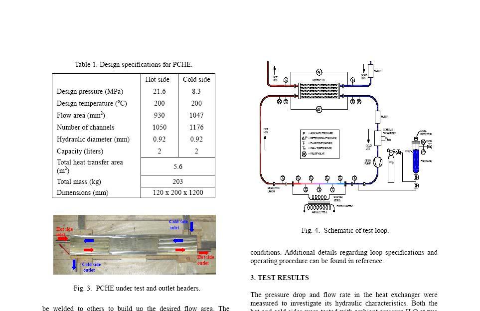
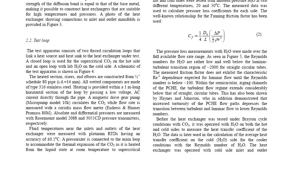
165 15

166 153

167 154

168 155

169 156

170 157