Rapid assessment of the marine primary productivity trends in the Arctic Ocean and its surrounding seas

Transcription

1 Rapid assessment of the marine primary productivity trends in the Arctic Ocean and its surrounding seas ACTUS inc. and WWF Final version March 2011

2 Table of Contents Abstract Introduction Methodology Satellite-based primary production estimation Statistical analysis Identification of the most productive pixels Trend analysis Results and discussion Pan-Arctic scale Total productivity Decadal trends Ecoregional scale Overview of all ecoregions Beaufort Sea continental coast and shelf Laptev Sea Conclusions...27 Glossary...30 References...31 Appendix...34 List of Figures Figure 1: Yearly primary production rates estimated using 13 years SeaWiFS images...9 Figure 2: Total annual primary production estimates during the SeaWiFS Era...11 Figure 3: Trends in PP calculated using the non parametric method proposed by Zhang et al. (2000) Figure 4: Anomaly in total PP at the pan-arctic scale (black), and anomaly explained by OC variability alone (grey) and light available for photosynthesis alone (blue) Figure 5: The relationship between the anomaly explained by OC and light availability Figure 6: Figure 6 - Monthly decompose PP anomaly at the pan arctic scale...15 Figure 7: Total annual primary production estimates during the SeaWiFS era for each ecoregion considered by RACER...19 Figure 8: Total annual primary production estimates during the SeaWiFS era for each ecoregion considered by RACER...20 Figure 9: Total annual primary production estimates during the SeaWiFS era for each ecoregion considered by RACER...21 Figure 10: PP production rates of the Beaufort Sea (continental coast and shelf)...24 Figure 11: Monthly decomposed total PP time series of the Beaufort Sea...25 Figure 12: PP trends of the Beaufort Sea computed using TSA...26 Figure 13: PP production rates of the Laptev Sea...27 Figure 14: Monthly decomposed total PP time series of Laptev Sea for all pixels (blue) and the 10% most productive pixels (black) Figure 15: PP trends of the Laptev Sea computed using TSA. Only pixels with significant trend (90% confidence level) are plotted

3 List of Tables Table 1: Comparison between satellite derived PP rates and published PP rate by Sakshaug 2004 (His table 3.7)...10 Table 2: Summary of the statistics of the mean annual PP rates (gc m-2 y-1) of each ecoregion Table 3: Main drivers controlling the inter-annual variability of total annual PP for each ecoregion Table 4: Trend analysis for each ecoregion following the Zhang et al. (2000) method

4 Abstract A 13-years time series of SeaWiFS imagery was employed to estimate the primary productivity (PP) rates taking place in the Arctic Ocean and its surrounding seas. The objective is to identify regions of biological interest and to assess how they are responding to the recent climate changes. A semi-analytic PP model ingesting satellite observations of cloud cover, sea ice concentration (SIC) and ocean inherent optical properties as determined ocean color (OC) measurements were employed to assess PP in both phytoplankton-dominated and colored dissolved organic matter (CDOM)-dominated waters. A preliminary validation suggested that the model produced PP rates within the range observed in situ over the arctic interior shelves, but may be underestimating PP in other regions. Unlike the previous satellite-based PP estimates, our model shows realistic estimates over the continental shelves supporting the necessity of using semi-analytical approaches to estimate both chlorophyll-a (CHL) concentration and diffuse attenuation coefficient to minimize the CDOM contamination. Hot-spots of high productivity, identified at the ecoregional scale, were found in areas influenced by large arctic rivers, in the marginal ice zone, at shelf breaks or in straits. A statistically significant trend in the temporal variation of PP was found at the pan-arctic scale (5.05 Tg C y -1). To explain the sources of this variation, the PP model was run several times with different input parameters set as constant. It was found that the main parameter that controlled the temporal trend reported above was the changes in OC (2.88 Tg C y-1). The second most important parameter (1.1 Tg C y-1) was SIC which incorporates light availability for photosynthesis through measurements of the shrinking of the sea ice cover. The ecoregional trends analysis indicates that both type of changes (OC versus SIC) operate in different proportions among regions. In general, increasing light availability explained most of the increase in PP over the arctic interior shelves, while changes in biomass are responsible for the increase in PP in permanently open waters. Although positive trends were observed in most ecoregions, significant negative trends were also observed in regions that are normally recognized for their great biological importance. This is the case with the North Water Polynya in the Canadian Arctic where the decrease in PP reaches as much as 5.6 gc m-2 y-1, corresponding to a >100% relative decrease in PP over 13 years. These results suggest that major environmental changes, yet not well understood, can locally have negative impacts on the marine ecosystem productivity. Finally, a more detailed analysis at ecoregional scale was exemplified at two ecoregions : the Beaufort Sea - continental coast and shelf and the Laptev sea. 4

5 1. Introduction This study takes place as part as RACER a project of WWF s Global Arctic Program that seeks to identify important places in the Arctic in the face of rapid climate change. RACER stands for Rapid Assessment of features and areas for Circum-arctic Ecosystem Resilience in the 21st Century. The ultimate goal of RACER is to develop the analyses that will identify some of the key places that will remain important for the well-being of Arctic ecosystems and human communities as we experience climate change. The RACER premise has been that if such places can be identified and given conservation attention when making decisions on land and marine use, then healthy Arctic ecosystems will stand a chance of being conserved and therefore be able to better adapt to rapid climate change - a process known as building resilience. The current study considers the marine realm of the Arctic. The Arctic ocean and is surrounding seas are among the most affected marine regions of the planet by global warming. The impacts of these changes on the marine ecosystems are already measurable from field-based (e.g. Grebmeier et al., 2006; Coyle et al., 2008; Li et al., 2009; Lalande et al, 2009) and satellitebased studies (e.g. Arrigo et al., 2008; Kahru et al., 2011). While the increase in primary productivity (PP) have been attributed to longer growing season resulting in enhanced light availability for photosynthesis (e.g. Arrigo et al., 2008), changes in environmental forcing of nitrate supply to the surface waters have been recently proposed as the main driver of the PP change in seasonally-ice free waters (Tremblay and Gagnon, 2009). If pan-arctic marine ecosystem is likely to be more productive as a result of declining sea ice extent and thickness, environmental forcing can evolved be very differently from a region to another with unknown effect on the productivity at the local scale. Satellite ocean-color radiometry is a powerful tool to detect the responses of the marine ecosystem productivity to changes in their physical environment. It provides quantitative assessment of the biological state of the surface ocean at synoptic and temporal scales inaccessible from traditional field observations. Among geophysical products derived from ocean-color data, chlorophyll-a (CHL), the pigment that is responsible for the photosynthesis of organic carbon in the ocean, is the most important when assessing the oceanic net PP. The main objective of this study was to assess the primary productivity of the arctic waters in order to identify regions of high biological productivity. We assume that the most productive region are also the most important in terms of their ecological functions in the marine food-web and in terms of biodiversity. Our assessment also focused on the temporal evolution of the marine PP since the launch of the Sea Wide Field-of-View Sensor (SeaWiFS) in August 1997, and try to identify the drivers of changes if any were detected. The main objective of this document is to present the methodological basis of our assessment and present our most important findings. Statistical spatial and temporal analysis and various maps of PP rates and trends were produced for the pan-arctic scale and for each ecological region of interest ( ecoregion ) defined by RACER. Only a fraction of the results will be presented and discussed here. The readers are referred to an Appendix for the complete results. 5

6 2. Methodology 2.1. Satellite-based primary production estimation Satelite-based primary production estimates are usually developed for blue ocean waters (e.g. Antoine et al., 1996; Behrenfeld and Falkowski 1997) for which bio-optical properties can be predicted from the phytoplankton biomass alone (case 1 waters; Morel and Pieur, 1977). In optically complex waters, like most waters found on the arctic shelves (Bélanger et al. 2008), a semi-analytical approach is needed to account for the spectral nature of light transmission, which is driven by phytoplankton and covarying water constituents as well as by all other optically active components that vary independently from phytoplankton (e.g. Platt et al. 1988, Sathyendranath et al. 1989, Morel 1991). For this study, a high-resolution satellite-based spectral radiative transfer model for a coupled atmosphere-ocean system has been implemented in Fortran 90 to quantify primary production. Details on the implementation of the model can be found in the Algorithm Theoretical Basis Document (Bélanger and Babin, in preparation 2011; ATBD) Briefly, spectral incident downwelling irradiance Ed(0-,,t) was computed at 5-nm resolution every 3-hours. Inputs for the atmospheric radiative transfer code (Ricchiazzi et al., 1998) are the solar zenith angle, the total ozone concentration, the cloud fraction over the pixel and the cloud optical thickness. The latter three parameters were obtained from the International Satellite Cloud Climatology Project (ISCCP) (Zhang et al., 2004). Sea viewing Wide field-of-view (SeaWiFS) Level 3 monthly fully-normalized spectral water-leaving reflectance (Rrs) at 412, 443, 490, 510, 555 and 670 nm were obtained from the NASA GSFC ( The Rrs data are binned at a 9.28-km resolution grid. Inherent Optical Properties (IOPs), namely the total absorption and backscattering coefficients, were estimated from Rrs( ) using a quasi-analytical algorithm (QAA) (Lee et al., 2002). The in-water spectral diffuse attenuation coefficient Kd( ) averaged over the euphotic zone was modeled following the approach of Lee et al. (2005a). Kd( ) was used to propagate Ed(z, ) throughout the water column. This was achieved at twelve depths from the surface to 0.1% level of the incident light. These calculations are necessary to account for detrital and dissolved organic matter absorption which are known to be abundantly present over the Arctic shelves (Bélanger et al., 2008, Siegel et al 2005). Daily PP rates were calculated using a photosynthesis-irradiance model (i.e., P vs E curve): (eq. 1) Chlorophyll a concentration (CHL; in mg m-3), photosynthetically usable radiation (PUR, in mol quanta m-2 s-1), the light-saturated CHL-normalized carbon fixation rate ( ; in mg C (mg CHL)-1 h-1), and the saturation irradiance (Ek, mol quanta m-2 s-1) are needed for the calculation of PP at each depth. CHL was derived from ocean color (OC) data by applying the GSM semianalytical model (Garver and Siegel, 1997; Maritorena et al, 2002), on images obtained from the MEaSUREs project. PUR was calculated at each time step and depth using : 6

7 (eq. 2) where aphyto( ) is the spectral phytoplankton absorption coefficient (in m -1), and is the spectral scalar irradiance calculated using the eq. 17 of Morel (1991) : (eq. 3) where at( ) is the total absorption coefficient obtained from the QAA applied to SeaWiFS data. aphyto( ) was calculated using an empirical statistical relationship established between CHL and aphyto( ) using prior measurements performed in the western Arctic Ocean (Matsuoka et al., 2007). Ek was modeled using the Arrigo et al. (1998) model which was developed for high latitudes, while was assumed constant, 2.0 mg C (mg CHL)-1 h-1, an average value based on field measurements in Arctic waters (Harrison and Platt, 1986; Sakshaug and Slagstad, 1991). The PP model was designed to produce an estimation of PP at every pixel where OC data are available. For each ocean pixel, a check is made to determine if OC data of the current month is available. If no data is available for that month, then it is checked whether the pixel had been previously documented during the 13 years of OC observations, i.e. in the monthly climatology. The monthly OC climatology was computed using the median values of the monthly IOPs and CHL for each pixel (see ATBD). If OC data is available, the daily PP is computed for each day of the month. The daily production rate of the pixel is adjusted as a function of the fraction of open water pixels, (1-SIC) where SIC is the sea ice concentration. Satellite-derived SIC was obtained from the National Snow and Ice Data Center (NSIDC). SIC is estimated from passive microwave data of the SSMI ( ) and AMSR-E sensors (2007 to present) using the NASA team algorithm (Cavallieri et al., 1992; Cavallieri and Comiso 2000). Daily SIC pixels are distributed over a polar stereographic grid of 25-km resolution Statistical analysis Identification of the most productive pixels Hot-spots of PP were identify at the ecoregional scale using the 90th percentile. The 90th percentile value for each study-unit was calculated by the aggregate function (for each studyunit) and the quantile function probability = 0.9) of the R statistical software package (R Development Core Team, 2011). The pixels with PP rates above the 90th percentile value were consider as the most productive pixels Trend analysis The trends in yearly PP over the 13 years of SeaWiFS time series was calculated at every pixel using a prewhitened nonlinear trends estimator developped by Zhang et al (2000). It is nonparametric method that removes autocorrelation from the time series before calculating the trend using the Theil-Sen approach (TSA; Sen slope). The function zyp.zhang implemented in R was used. The Mann-Kendall test for trend significance is then run on the resulting time series. 7

8 The decomposition of the time series into three distinct components was done with the stl function of R ( This is a filtering procedure that uses the loess method to breakup a time series into its seasonal (cyclic), trend and irregular (residual) components (Cleveland et al., 1990). The seasonal component is estimated through the loess smoothing of the seasonal sub-series. A time window of 12 months was used, providing the seasonal trend for all months separately. The seasonal component is removed from the total and the remainder was filtered again to eliminate the irregular component, yielding the local trend. The algorithm iterates the process twice. 3. Results and discussion 3.1. Pan-Arctic scale Total productivity Total productivity of the arctic waters, as defined here by the RACER project, is on the average, 412 ± 25 Tg C y-1 (± standard deviation). This value is similar to that reported by Pabi et al. (2008) and Arrigo et al. (2008), but the area covered by our study includes sub-arctic regions such as the Bering Sea, the Hudson Bay and the northern Labrador Sea. When we only consider the circumpolar waters (latitude > N), the total productivity is 240 Tg C y-1, which is nearly 2-times lower than the estimates published by Pabi et al. (2008). This difference arises mainly from the lower CHL values obtained using the semi-analytical model (GSM) as compared to those of Pati et al. (2008) that are empirically determined (Siegel et al. 2005). Figure 1 shows the spatial distribution of the PP rates (g C m -2 y-1) averaged over the SeaWiFS era. Hotspots of high productivity (>100 g C m-2 y-1) are located over the shelves located near the mouths of large rivers : Yenesei and Ob in the Kara Sea, Lena in the Laptev Sea, Mackenzie in the Beaufort Sea and the James Bay which is located south of Hudson Bay. Despite the fact that our model accounts for non-phytoplankton absorption through the use of GSM for CHL and QAA for IOPs and Kd, we cannot exclude some remaining contamination on the PP values by river runoff. In contrast, other hotspots of PP ( g C m -2 y-1) can be found away from zones influenced by river runoff (case 1 waters). That includes the Barents shelf and the Bering Strait, which are known has the most productive region of the Arctic (Sakshaug 2004; Carmack et al. 2006), and the Cape Bathurst Polynya, the North Water Polynya (NOW), the Iceland shelf and the southern Greenland coast. High production in these regions is expected due to favorable environmental conditions such as bathymetrically or wind-forced upwellings and the presence of fronts between water masses. For example, the NOW polynya hosts very intense phytoplankton spring-summer blooms (Lewis et al., 1996), with a total annual productivity reaching as much as 250 g C m -2 y-1 (average = 150 g C m-2 y-1), (Klein et al., 2002). This value is much higher than our satellitebased estimation (~75 g C m-2 y-1). This may have arisen from both the low GSM CHL retreival and/or low used in the PP model (eq. 1; 2 mg C (mg CHL)-1 h-1). Similar remarks can be made when comparing our satellite-based PP rates with in-situ measurements reported by Hill and Cota (2005) for the Chukchi shelf, i.e g C m-2 y-1 vs 40 g C m-2 y-1, but are comparable with the value of 19.8 g C m-2 y-1 that was measured on the basin s edge (as compared with our g C m-2 y-1). A preliminary validation of our PP model was made through a comparison between our satellite PP estimates and historical values compiled for various Arctic regions by Sakshaug (2004) (Table 1). With the exception of the White Sea, the satellite rates are similar or lower than the in- 8

9 situ estimates. Our PP rates calculated over the arctic interior shelves are within the ranges of in situ measurements (< 150 g C m -2 y-1). A visual inspection of the PP rates reported by Arrigo et al (2008) over most of the shelves for 2006 and 2007 reached >150 g C m -2 y-1, which is unlikely based on in situ measurements. In addition, Vetrov et al (2008) repported that standard SeaWiFS CHL in the Laptev sea are 2.5 to 5-fold higher than actual in situ measurements of CHL. This overestimation by standard CHL algorithm are likely a results of the massive input of CDOM by the Lena river (Holmes et al., 2011). Recent findings on the Beaufort shelf confirmed the poor performance of empirical algorithm in the arctic waters (Bélanger et al., in prep; Ben Mustapha et al., 2011, submitted manuscript). These results support the benefit of using semianalytical approaches to estimate both CHL and diffuse attenuation coefficients, which minimize the contamination by non-covarying material such a CDOM in coastal waters. Considering the Pan Arctic scale, our model underestimates the total PP by more than a 2-fold factor (464 versus 1169 Tg C y-1). This can be explained by the presence of sub-surface chlorophyll-a maximum (SCM) that is inaccessible directly from space but hosts significant primary productivity. Indeed, a recent study indicates the near-ubiquity of SCM in the Canadian Archipelago (Martin et al 2010). Mitchell et al. (1991) already discussed this inherent limitation based on coincident in situ and Coastal Zone Color Scanner (CZCS) measurements in the Barents Sea in the early 80 s. More importantly, the Arctic SCM tends to be located between 3 to 10% light levels, contrasting markedly with the global ocean SCM that usually is below the 1% light level (Uitz et al., 2006). Consequently, SCM accounts for a significant proportion of the PP (Martin et al., 2010; Luchetta et al 2000). New approaches are needed to predict the vertical profile of CHL. Clearly, an extensive validation of all the components of the PP model is needed to provide an accurate PP estimation at the Pan-Arctic scale. Figure 1: Yearly primary production rates estimated using the 13 years of SeaWiFS observations 9

10 Table 1: Comparison between satellite derived PP rates and those in the table 3.7 of Sakshaug (2004). Area (103 km2 ) PP rate (g C m-2 y-1) Total PP (Tg y-1) Literature Satellite mean ± st. dev. Literature Satellite mean ± st. dev. >11 5±1 >50 22 ± 5 Central Deep Arctic 4489 Arctic Shelves: 5027 Barents Sea 1512 < ± 6 < ± 10 White Sea ± ± 2 Kara Sea ± ± 4 Laptev Sea ± ± 4 East Siberian Sea ± ± 4 Chukchi Sea > ± ± 2 Beaufort Sea ± ± 0.5 Lincoln Sea ± <1 Canadian Archipelago ± ± 0.2 Atlantic Sectors 4600 Baffin Bay ± ± 2 Hudson Bay ± ± 2 Greenland Sea ± ± 3 Labrador Sea ± ± 6 Norwegian Sea ± ± 4 Bering Shelf + Oceanic > ± 2 > ± 6 TOTAL Arctic and subarctic seas ± 53 10

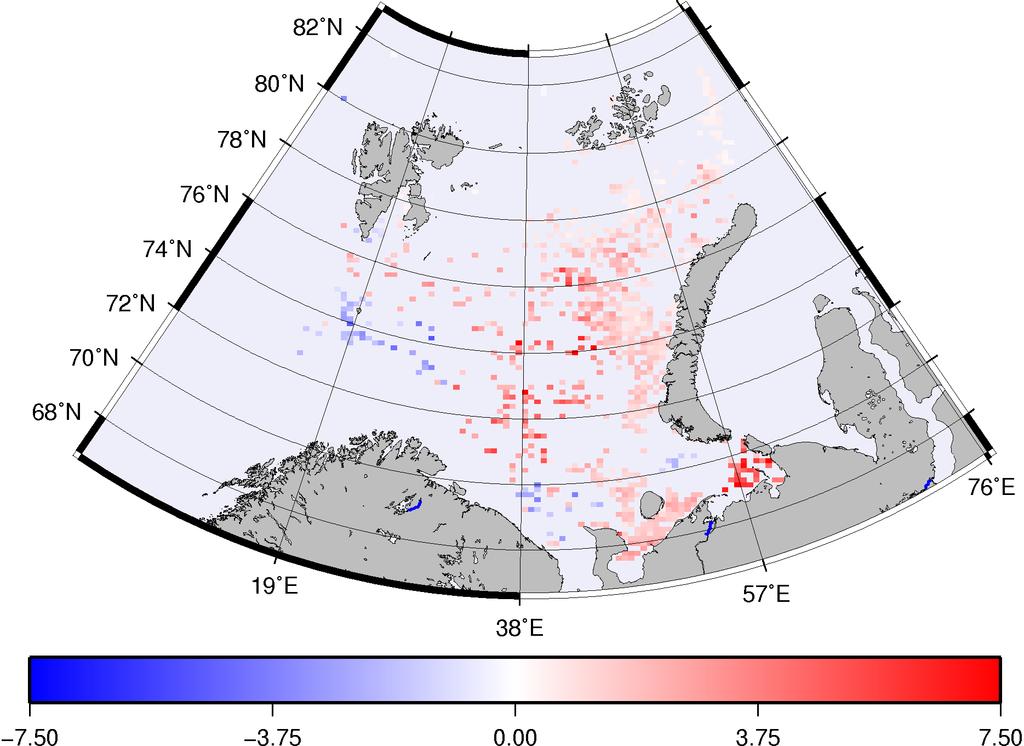
11 Decadal trends Despite the limitations mentioned above, it can be assumed that the error made on the PP estimation at the local scale (pixels) is similar from one year to another. With this assumption, calibrated satellite-based time series analysis can still reveal significant spatial patterns and temporal trends in the biological productivity of the marine ecosystems (e.g. Pabi et al., 2008; Arrigo et al. 2008; Perrette et al 2011; Kahru et al 2011). For the SeaWiFS Era, the lowest productivity was observed in 1998 (381 Tg C y-1), while 2010 recorded the highest productivity (469 Tg C y-1), representing an increase of ~88 Tg C (23%) in 13 years (Figure 2). Figure 2: Total annual primary production estimates during the SeaWiFS Era (sum of all RACER marine study units). A controlled run (thin line) was made with constant sea ice and cloud conditions to isolate the variability that is strictly due to changes in ocean color properties (i.e. IOPs and CHL). See text for details. Examination of the spatial patterns in the PP trends across different Arctic regions reveals that the change in total production rates is not spatially homogeneous (Figure 3). The trends are positive (red) in many seasonally ice-free regions: eastern Barents shelf, Siberian shelves (Kara and east siberian seas), western Mackenzie shelf, Bering strait. This is coherent with the results reported by Arrigo et al (2008) who showed that a longer growing season can explain most of the PP increase around the central ice pack. Further south, a very strong increase in PP is also observed on the southern part of the East Greenland shelf. However, positive trends were also found in permanently open waters. This is the case of the southern Iceland shelf and the western Beging Sea. Changes in these regions can only be explained by a change in the biomass (CHL). 11

12 Notable exceptions where significant negative trends (95% confidence level) can be found in the two most productive polynyas of the Canadian Arctic Archipelago: the NOW and Cap Bathurst. Most of the Northeast Bering Sea, the Fram Stait and the southern Greenland shelf show significantly negative trends in their productivity. Interestingly, evidences of changes in the former region have been reported by Coyle et al. (2008), who observed a trend toward an increasing stratification of the water column resulting from the sea surface warming. Figure 3: Trends in PP calculated using the non parametric method proposed by Zhang et al. (2000). Only pixels with significant trends at the 95% confidence level (Mann-Kendall test) are shown. Recent studies reported that changes sea ice extent and longer phytoplankton growing season were the main drivers of the observed PP trends (Arrigo et al. 2008), and that the earlier opening of water results in earlier phytoplankton blooms (Kahru et al., 2011). In contrat, Tremblay and Gagnon (2009) recently proposed that changes in nutrients supply, in particular nitrogen, are the main drivers of PP changes in the seasonally ice-free waters. Changes in OC are related to modifications in marine biological-physical coupling resulting in changes of the timing, intensity and duration of phytoplankton blooms. Over the arctic shelves, OC changes can also result from the variability in freshwater inputs by rivers, which are known to be changing with time (Peterson 12

13 et al., 2006). In contrast, sea ice and cloud conditions control the amount of radiant energy available for photosynthesis. In order to better understand the observed variations, one needs to isolate the impact of changes in OC, SIC and cloud conditions and analyse separately their influence on PP. To test the hypothesis that significant changes in OC can be detected, the PP model was forced to use the climatology ( ) for both sea ice and atmospheric conditions (controlled run in Fig. 2 and the grey curve in Fig. 4). The controlled run sets the incident irradiance constant with time, allowing to evaluate the effect of changes in OC on the total PP. Similarly, the effect of changes in the amount of light available for photosynthesis were isolated by forcing the model to use the IOPs and CHL climatologies for every year, while keeping the SIC and cloud conditions variable over time. Figure 4 shows the results of the controlled runs, as compared with the actual trend in units of absolute total PP anomaly. As expected, the sum of anomalies of the two controlled runs is equal to the actual PP anomaly within a few percent. Therefore one can explain quantitatively the fraction of the actual anomaly that can be explained by variations in OC and light availability. For example, total PP anomaly in 1998 reached Tg C y-1, out of which 69% (21 Tg C y-1) is explained by OC variability and the remainder is explained by a reduction in light availability for photosynthesis. In contrast, the 2005 anomaly (24.6 Tg C y -1) was explained by an increase in light availability (14 Tg C y-1), which was more important than that resulting from OC changes (10.6 Tg C y-1). The sharp increase of 2010 (+57 Tg C y -1) is largely explained by an increase in phytoplankton biomass (+42 Tg C y-1) rather than a change in light availability (+13 Tg C y -1). The trend estimator (TSA) reached 5.05 Tg C y-1 (p < 0.1), 2.88 Tg C y-1 (p < 0.05) and 1.1 Tg C y-1 (p = 0.45) for total, OC, and light availability anomalies respectively. It was noticed that the PP anomalies resulting from OC and light availability were weakly correlated (r2 = 0.55), suggesting that a relationship may exist between the two variables (Fig, 5). In other words, when more (or less) light is available for photosynthesis (e.g. low SIC or cloud cover, longer growing season, blooms developing during longer days), a higher (lower) phytoplankton biomass can build-up. This correlation may be related to some physical forcings such as favorable wind-driven upwellings during lower sea ice conditions that replenish surface layer with nutrients (Carmack and Chapman., 2003; Tremblay and Gagnon 2009), or a change in the coupling between primary producers and higher trophic levels (Tremblay et al 2006). More research is needed for a better understanding of these results. Monthly PP anomalies reveals that the timing of the phytoplankton bloom has shifted toward earlier in the season. This is evidenced be the seasonal components of the decomposed time series (Fig. 6). Similarity between actual and controlled time series suggest that the changes were driven by shift in phytoplankton biomass. This observation is in accordance with Kahru et al. (2011). Interestingly, late season productivity (August) had also increased over time. Autumn phytoplankton bloom is a typical phenomena of temperate region when the summer water column stability that prevent nutrient replenishment is eroded by wind and radiative fluxes forcings. It is important to mention at this point that a large proportion of the area considered at the panarctic scale is not affected by seasonal sea ice. Consequently, in those permanently open waters, only OC and cloud cover can explain the inter-annual variability in total PP. In the next section trends in total PP will be explored at the scale of ecological regions. 13

14 Figure 4: Anomaly in total PP at the pan-arctic scale (black), and anomaly explained by OC variability alone (grey) and light available for photosynthesis alone (blue). Figure 5: The relationship between the anomaly explained by OC and light availability. 14

15 Figure 6: Monthly decompose PP anomaly at the pan arctic scale. 15

16 3.2. Ecoregional scale Overview of all ecoregions Table 2 ranks the 27 ecoregions from the most productive hot-spots to the least productive ones. Hot-spots are defines here as the 10 % most productive pixels of each ecoregion. The median was found to provide the most appropriate estimator considering the non-normality of the frequency distribution of PP. The most productive hot-spots are found on Arctic interior shelves where large rivers supply the surface waters with nutrients (Holmes et al., 2011) and where shelf breaks favour upwellings of nutrient-rich deep waters under reduced summer ice cover (Carmack and Chapman, 2003). Surprisingly, the inflow shelves, i.e. Chuckchi and Barents seas, do not rank above the interior shelves as expected (Sakshaug 2004; Carmack et al 2006). As mentioned above, absolute values should be interpreted with care in regions influenced by river runoff due to potential contamination by CDOM. It is however most likely that the identified hot-spots are locally the regions with most biological significance (for the exact position of these hot-spots, the reader is refer to the Appendix). Table 2: Summary of the statistics of the mean annual PP rates (gc m -2 y-1) of each ecoregion. Ecoregion Overall median #rank max #rank 90th percentile #rank Hot-spots median #rank White Sea # # # #1 Laptev Sea 34.0 # # # #2 Kara Sea 19.3 # # # #3 Iceland Shelf 66.7 # # # #4 Beaufort Sea - continental coast and shelf 31.0 # # # #5 Eastern Bering Sea 42.9 # # # #6 North and East Barents Sea 35.3 # # # #7 Northern Finnmark 56.0 # # # #8 Labrador Sea Basin 46.2 # # # #9 Northern Grand Banks Southern Labrador 34.3 # # # #10 Western Bering Sea 41.2 # # # #11 East Siberian Sea 8.3 # # # #12 Norwegian Sea 44.1 # # # #13 Norway and 16

17 Ecoregion Overall median #rank max #rank 90th percentile #rank Hot-spots median #rank West Greenland Shelf 30.1 # # # #14 Fram Strait 40.7 # # # #15 Hudson Complex 17.0 # # # #16 North Greenland 8.8 # # # #17 Northern Labrador 23.9 # # # #18 Baffin Bay -- Canadian Shelf 13.3 # # # #19 Chukchi Sea 9.1 # # # #20 East Greenland Shelf 14.2 # # # #21 Lancaster Sound 7.8 # # # #22 High Arctic Archipelago 2.11 # # # #23 Beaufort-AmundsenViscount_MelvilleQueen_Maud 5.08 # # # #24 Baffin Bay 8.6 # # # #25 Arctic Ocean--Pacific Basin 2.0 # # # #26 Arctic Ocean--Atlantic Basin 3.3 # # # #27 Figure 7 shows the total inter-annual PP variability for the 27 ecoregions considered by the RACER study. Each plot present the actual total yearly PP and the corresponding controlled run that isolates the impact of changes in the ocean color properties (as in Figs. 2 and 4). Comparison of the actual and controlled total PP helps to identify whether the inter-annual variability is driven by the variability of light availability, ocean color, or both (Table 3). The regions where PP is controlled almost exclusively by OC variability are also the largest in size and accounted for about 50% of the total pan-arctic PP. The trends for each ecoregion were assessed for both actual and controlled PP time series using the TSA (Table 4). Seven out of 27 ecoregions showed a significantly positive trends (95% confidence level) : Arctic Ocean-Pacific Basin, Beaufort-Amundsen-Viscount Melville-Queen Maud, Chuckchi Sea, Iceland Shelf, Kara Sea, West Bering Sea, White Sea. Only three of them, i.e. the Iceland Shelf, the West Bering Sea and White Sea showed a concurrent increase in phytoplankton biomass as suggested by the trend of the controlled run (Table 4). In the four other regions, the trend can be explained by an increase in light availability. 17

18 Table 3: Main drivers controlling the inter-annual variability (>80%) of total annual PP for each ecoregion. Light availability Ocean color Both Arctic Ocean (both Atlantic and Pacific Basins) Beaufort-AmundsenViscount-Melville-Queen Maud East Greenland Shelf East Siberian Sea High Arctic Archipelago Kara Sea Laptev Sea Lancaster Sound Fram Strait Iceland Shelf Labrador Sea Basin Northern Norway & Finnmark Norwegian Sea Western Bering Sea White Sea Baffin Bay Baffin Bay - Canadian Shelf Beaufort Sea - coast and shelf Chukchi Sea Eastern Bering Sea Hudson complex North Greenland North & East Barents Sea Northern Grand Banks Southern Labrador Northern Labrador West Greenland Shelf In contrast, the productivity decreased significantly in two ecoregions: Baffin Bay - Canadian Shelf and North Greenland. The Baffin Bay - Canadian Shelf hosts the NOW polynya, which is known as the most productive region of the high Arctic (Lewis et al. 1996; Sakshaug 2004). The North Greenland ecoregion comprises a part of the NOW polynya, the Nares strait, the Lincoln Sea and the North East Water (NEW) polynya. The highest negative trend of -5.6 gc m -2 y-1 ( < 0.005; sen slope) was observed just south of Smith Sound located north of the NOW polynya (78 N; 74 W) where an ice brigde usually forms in winter and stops the ice from the Arctic to flow in the polynya. Interestingly, the decrease in biomass is likely to be responsible for an important part of the decrease in the total annual PP in the northern Baffin Bay (negative, albeit statistically not significant trend of the controlled run; Table 4). A careful analysis of the annual PP trends in this region revealed that the productivity starts to decrease constantly after The reasons for this decrease are unknown, but the ice formation in Nares Strait and ice flow into the polynya changed dramatically since 2007 (Kwok et al 2010). Examination of satellite ocean images averaged over a 8-days period revealed that the ice bridge usually found in Smith Sound, between Greenland and Ellesmere island did not form in 2007, 2009 and 2010 (data not shown). These changes may be accompanied by changes in oceanic currents that would modify the composition and/or the water column stratification of water masses which, in turn, control the nutrients availability (Dumont et al., 2010). The significantly positive trends calculated from the controlled run suggests that changes in the OC data occurred in two regions: Hudson complex and Laptev Sea. The strong inter-annual variability in the sea ice over these regions explains why no significant trends were observed in terms of actual total annual PP. 18

19 Figure 7: Total annual primary production estimates during the SeaWiFS era for each ecoregion considered by RACER. A controlled run (thin line) was made with constant sea ice and cloud conditions to isolate the variability that is strictly due to changes in ocean color properties (i.e. IOPs and CHL). See text for details. 19

20 Figure 8: Total annual primary production estimates during the SeaWiFS era for each ecoregion considered by RACER. A controlled run (thin line) was made with constant sea ice and cloud conditions to isolate the variability that is strictly due to changes in ocean color properties (i.e. IOPs and CHL). See text for details. 20

21 Figure 9: Total annual primary production estimates during the SeaWiFS era for each ecoregion considered by RACER. A controlled run (thin line) was made with constant sea ice and cloud conditions to isolate the variability that is strictly due to changes in ocean color properties (i.e. IOPs and CHL). See text for details. 21

22 Table 4: Trend analysis for each ecoregion following the Zhang et al. (2000) method. P values were obtained from a Mann-Kendall test. Values in brackets are the lower and upper bound of the Sen slope estimators at 95% confidence interval. Numbers in bold characters indicate trends significant at 90% confidence level. Ecoregion Actual mean [lower,upper] P Controlled mean [lower, upper] P Arctic Ocean (Atlantic Basin) 0.01 [-0.08, 0.07] [0.00, 0.00] 1.00 Arctic Ocean (Pacific Basin) 0.07 [-0.01, 0.19] [-0.05, 0.04] 0.84 Baffin Bay - Canadian Shelf [-0.15, -0.04] [-0.11, 0.04] 0.19 Beaufort -cont. coast and shelf 0.10 [-0.04, 0.25] [-0.12, 0.02] 0.11 Beaufort-Amundsen-Viscount Melville-Queen Maud 0.11 [0.00, 0.22] [-0.03, 0.02] 0.84 Chukchi Sea 0.23 [0.03, 0.48] [-0.14, 0.22] 0.54 Baffin Bay 0.01 [-0.02, 0.05] [-0.04, 0.06] 0.63 East Greenland Shelf [-0.14, 0.08] [-0.03, 0.03] 0.85 East Siberian Sea 0.35 [-0.07, 0.74] [-0.06, 0.15] 0.13 Eastern Bering Sea [-1.10, 0.46] [-0.29, 0.41] 0.95 Fram Strait 0.06 [-1.30, 1.59] [-1.00, 2.15] 0.95 High Arctic Archipelago 0.01 [0.00, 0.03] [0.00, 0.00] 0.67 Hudson Complex 0.14 [-0.10, 0.52] [0.15, 0.39] 0.00 Iceland Shelf 0.15 [0.02, 0.29] [-0.01, 0.30] 0.09 Kara Sea 0.43 [0.17, 0.83] [-0.25, 0.29] 0.95 Labrador Sea Basin 0.22 [-0.16, 0.48] [-0.10, 0.46] 0.10 Lancaster Sound 0.00 [-0.04, 0.06] [-0.02, 0.02] 0.85 Laptev Sea 0.36 [-0.54, 1.00] [0.04, 0.40] [-0.11, -0.03] [-0.10, 0.05] [-0.73, 2.48] [-0.63, 1.19] 0.67 North Greenland North and East Barents Sea 22

23 Table 4 - Continued Ecoregion Actual [lower, mean, upper] P Controlled [lower, mean, upper] P Northern Grand Banks Southern Labrador 0.01 [-0.02, 0.06] [-0.01, 0.06] 0.30 Northern Labrador [-0.16, 0.14] [-0.08, 0.05] 0.50 Northern Norway & Finnmark [-0.26, 0.27] [-0.22, 0.23] 0.76 Norwegian Sea [-0.46, 0.26] [-0.35, 0.36] 0.85 West Greenland Shelf 0.12 [-0.01, 0.24] [-0.11, 0.13] 0.85 Western Bering Sea 0.55 [0.06, 1.40] [0.17, 1.24] 0.01 White Sea 0.18 [-0.06, 0.43] [-0.03, 0.36] Beaufort Sea continental coast and shelf The continental coast and shelf of the Beaufort Sea is characterized by two important features that controls its primary productivity (Figure 10) : 1) the large freshwater input of the Mackenzie River over the western part of the shelf and 2) the coastal upwelling of Pacific waters near the Cape Bathurst over the eastern part of the shelf. The high PP rates (> 100 gc m -2 y-1) estimated near the river mouth may be overestimated due to CDOM absorption that may have been confounded with CHL. Nevertheless the PP rates on most of the shelf (30-90 gc m -2 y-1) were somewhat similar or higher than the in situ measurements (30-70 gc m-2 y-1) performed in the 80 s (Macdonald et al., 1987; Carmack et al., 2004). In addition, the most productive pixels located at the mouth of the Mackenzie river produced ~1 Tg C y -1. The nitrogen requirement to support this production, assuming a Redfield C:N ratio of 6.625, is 0.15 Tg N. The Mackenzie River alone would supply to about 20 to 40% of this N requirement based on the most recent estimates of nutrient fluxes into the Arctic Ocean (Holmes et al., 2011). The monthly PP time series analysis revealed that a decrease in productivity occurred during the period, and then increased until 2010 (Fig. 11). As a result, no significant trend can be distinguished for the whole area (Table 4). The inter-annual variability in PP in this region was mostly explained by light availability (Fig. 7; Table 3). It should be noted that exceptional weather conditions were observed in this region in 1998 when strong and persistent southeasterly winds during the spring-summer season transported the sea ice cover way offshore in early June (Comiso et al., 2003). This may explains why a negative trend was observed at the beginning of the time series. The 10% most productive pixels showed somewhat a higher interannual variability than the whole region, with no clear trends. Figure 12 depicts the spatial variability in the PP trends. Significantly positive (90%) trends were found west of the Mackenzie delta and along the Alaskan coast. Only a few pixels showed significantly negative trends over the eastern part of the Mackenzie shelf, near the Cape Bathurst polynya. Interestingly, the area centered on 140 W-70.5 N is not far from Mackenzie Trough where upwellings are frequent. 23

24 Primary Production (gc m-2 y-1) Figure 10: PP production rates of the Beaufort Sea (continental coast and shelf). Contour lines indicate the 10% most productive pixels based on the 90th percentile analysis (see the method section) 24

25 Trends in PP (gc m-2 y-1) Figure 11: PP trends of the Beaufort Sea (continental coast and shelf) computed using TSA. Only pixels with significant trend (90% confidence level) are plotted Laptev Sea As in the Beaufort Sea, the annual primary productivity of the Laptev Sea is highest near the freshwater input by the rivers (Fig 13). This hot-spot of PP ranks second overall (Table 2). Indeed, PP rates reaching 150 gc m-2 y-1 were found downstream of the Lena River which is the largest Arctic River. The Lena river is arguably an important source of nutrients that controls the PP of this oligotrophic region (Holmes et al., 2011). However, to support the total productivity estimated in the most productive zone (~5 Tg C y -1), 0.75 Tg of nitrogen would be required. The total annual influx of total dissolved nitrogen (TDN) by the Lena River would support at most 22% of the total requirement (0.17 Tg N y -1, Holmes et al. 2011). A positive trend in the TDN flux by the Lena river have been observed from 2004 to 2009 (Holmes, personal communication, March 2011). Nevertheless, our PP estimations fall within the range reported by Vetrov et al (2008). The authors calculated PP from empirical relationships derived from in situ measurements of CHL and PP. Their satellite-based CHL estimations were based on SeaWiFS and MODIS images after an ad hoc adjustment of the CHL magnitude based on their extensive in situ data set. For example, standard SeaWiFS CHL was multiplied by a factor of 0.2 and 0.4 for pixels located at latitudes <75.3 N and between N respectively. In other words, the standard SeaWiFS algorithm overestimates CHL by a factor of 5 in coastal waters and ~2.5 at the shelf break. These results, therefore suggest that using the GSM algorithm for the CHL retrieval prevents us from a severe overestimation of PP in these optically complex waters, but the overestimation cannot be totally avoided. 25

26 Figure 12: Monthly decomposed total PP time series of the Beaufort Sea (continental coast and shelf) for all pixels (blue) and the 10% most productive pixels (black). Again, light availability seems to be the main factor controlling the inter-annual variability in total PP of the Laptev Sea (Fig 8; Table 3). Much like for the Beaufort Sea, no significant trend was observed due to the high inter-annual variability in the SIC (Table 4). However, a significantly positive trend in PP (0.23 Tg C y-1) of the controlled run indicates a change in the OC that may be occurring in this region (Table 4). Recently Lalande et al (2009) showed increased particles flux in the deep basin during the reduced sea ice conditions of 2007, which was corroborated by satellite observations (Fig 14). The 10% most productive pixels showed an inter-annual variability that was very much similar to the whole region, with no clear trends. In fact, significant positive trends, though highly scattered spatially, were found in the southeastern part of the shelf (Fig 15). 26

27 Primary Production (gc m-2 y-1) Figure 13: PP production rates of the Laptev Sea. Contour lines indicate the 10% most productive pixels based on the 90th percentile analysis. 4. Conclusions Methods providing satellite-based estimations of the arctic PP are still at their early phases. In the current study we employed an OC algorithm that should in theory have a reduced uncertainty of CHL (GSM) and that accurately estimates the light propagation in the ocean (Lee et al., 2005b). Comparison with published PP rates (Sakshaug 2004) suggests that PP may be underestimated in several regions. Among the possible reasons are the biased CHL estimates provided by satellite OC data and the lack of consideration of the deep chlorophyll maximum that may be providing a significant contribution to PP (Martin et al., 2010; Luchetta et al 2000). Despite these inherent limitations, the satellite-based PP model is an efficient tool to detect changes in the rapidly evolving Arctic marine environment. Future works need to 1) address the technical aspects of the PP model and improve its performance, 2) assess the accuracy of the PP model based on a thorough validation based on in situ PP measurements, and 3) to relate the observed PP anomalies to the variations in climate as observed by other, independent measurements of the sea surface temperature and wind forcing. 27

28 Figure 14: Monthly decomposed total PP time series of Laptev Sea for all pixels (blue) and the 10% most productive pixels (black). 28

29 Trends in PP (gc m-2 y-1) Figure 15: PP trends of the Laptev Sea computed using TSA. Only pixels with significant trend (90% confidence level) are plotted. 29

30 Glossary AMSR-E Advanced Microwave Scanning Radiometer for EOS aphyto The phytoplankton absorption coefficient,m-1 at The total absorption coefficient, m-1 CDOM Chromophoric dissolved organic matter CHL Chlorophyll-a concentration, mg m-3 CZCS Coastal Zone Color Scanner Ed The downwelling irradiance, W m-2 E0 The scalar irradiance, W m-2 Ek The saturation irradiance, mol quanta m-2 s-1 GSM The Garver-Siegel-Maritorena OC algorithm IOPs Inherent optical properties, namely the absorption and backscattering coefficients, m-1 ISCCP International Satellite Cloud Climatology Project Kd The diffuse attenuation coefficient, m-1 MODIS Moderate Resolution Imaging Spectroradiometer NEW North East Water polynya NOW North Water polynya NSIDC National Snow and Ice Data Center OC Ocean Color PBmax The light-saturated CHL-normalized carbon fixation rate, mg C (mg CHL)-1 h-1 PP Primary production, g C y-1 PUR The photosynthetically usable radiation, mol quanta m-2 s-1) QAA The Quasi-analytical OC algorithm (Lee et al., 2002) Rrs Fully-normalized water-leaving reflectance, sr-1 SCM The sub-surface chlorophyll-a maximum SeaWiFS Sea-Viewing Wide Field-of-view SIC Sea ice concentration SSMI The Special Sensor Microwave/Imager 30

31 TDN Total dissolved nitrogen TSA The Sen slope as calculated following the Theil-Sen approach. References Antoine, D., A. Morel, and J. M. André (1996), Oceanic primary production : II. Estimation at global scale from satellite (Coastal Zone Color Scanner) chlorophyll, Global Biogeochem. Cycles, 10(1), Arrigo, K. R., D. Worthen, A. Schnell, and M. P. Lizotte (1998), Primary production in Southern Ocean waters, J. Geophys. Res., 103(C8), Arrigo, K. R., G. van Dijken, and S. Pabi (2008), Impact of a shrinking Arctic ice cover on marine primary production, Geophys. Res. Lett., 35(19), L Behrenfeld, M. J., and P. G. Falkowski (1997), Photosynthetic rates derived from satellite-based chlorophyll concentration, Limnol. Oceanogr., 42(1), Bélanger, S., M. Babin, and P. Larouche (2008), An empirical ocean color algorithm for estimating the contribution of chromophoric dissolved organic matter to total light absorption in optically complex waters, J. Geophys. Res., 113(C4), 1-14, doi: /2007jc Carmack, E. C., and D. C. Chapman (2003), Wind-driven shelf/basin exchange on an Arctic shelf: The joint roles of ice cover extent and shelf-break bathymetry, Geophys. Res. Lett., 30(14), Carmack, E. (2006), Progress in Oceanography Climate variability and physical forcing of the food webs and the carbon budget on panarctic shelves, Progress in Oceanography, 71, , doi: /j.pocean Carmack, E. C., R. W. MacDonald, and S. Jasper (2004), Phytoplankton productivity on the Canadian Shelf of the Beaufort Sea, Mar. Ecol. Progr. Series, 277, Cavalieri, D., and J. Comiso (2000), Algorithm Theoretical Basis Document for the AMSR-E Sea Ice Algorithm, Revised December 1, Cavalieri, D. J. et al. (1992), NASA Sea Ice Validation Program for the Defense Meteorological Satellite Program Special Sensor Microwave Imager: Final Report,, Washington, D.C. Cleveland, R. B., W. S. Cleveland, J. E. McRae, and I. Terpenning (1990), A Seasonal-Trend Decomposition Procedure Based on Loess, J of Official Statistics, 6, Comiso, J. C., J. Yang, H. Susumo, and R. A. Krishfield (2003), Detection change in the Arctic using satellite and in situ data, Journal of Geophysical Research-Oceans, 108(C12), Coyle, K. O., A. I. Pinchuk, L. B. Eisner, and J. M. Napp (2008), Zooplankton species composition, abundance and biomass on the eastern Bering Sea shelf during summer : The potential role of water-column stability and nutrients in structuring the zooplankton community, Deep-Sea Research, 55, Dumont, D., Y. Gratton, and T. E. Arbetter (2010), Modeling Wind-Driven Circulation and Landfast Ice-Edge Processes during Polynya Events in Northern Baffin Bay, Journal of Physical Oceanography, 40(6), Garver, S., and D. Siegel (1997), Inherent optical property inversion of ocean color spectra and its biogeochemical interpretation 1. Time series from the Sargasso Sea, J. Geophys. Res., 102, Grebmeier, J. M., J. E. Overland, S. E. Moore, E. V. Farley, E. C. Carmack, L. W. Cooper, K. E. Frey, J. H. Helle, F. A. McLaughlin, and S. L. McNutt (2006), A Major Ecosystem Shift in the Northern Bering Sea, Science, 311 (5766 ), Harrison, W. G., and T. Platt (1986), Photosynthesis-irradiance relationships in polar and temperate phytoplankton populations, Polar Biology, 5,

32 Hill, V., and G. Cota (2005), Spatial patterns of primary production on the shelf, slope and basin of the Western Arctic in 2002, Deep Sea Research Part II: Topical Studies in Oceanography, 52(24-26), Holmes, R. M. et al. (2011), Seasonal and Annual Fluxes of Nutrients and Organic Matter from Large Rivers to the Arctic Ocean and Surrounding Seas, Estuaries and Coasts, doi: /s Kahru, M., V. Brotas, M. Manzano-Sarabia, and B. G. Mitchell (2011), Are phytoplankton blooms occurring earlier in the Arctic?, Global Change Biology, 17(4), , Klein, B. et al. (2002), Phytoplankton biomass, production and potential export in the North Water, Deep-Sea Research, 49(22-23), Kwok, R., L. Toudal Pedersen, P. Gudmandsen, and S. S. Pang (2010), Large sea ice outflow into the Nares Strait in 2007, Geophysical Research Letters, 37(3), doi: /2009gl Lalande, C., S. Bélanger, and L. Fortier (2009), Impact of a decreasing sea ice cover on the vertical export of particulate organic carbon in the northern Laptev Sea, Siberian Arctic Ocean, Geophys. Res. Lett., 36, L21604, doi: /2009gl Lee, Z. P., M. Darecki, K. L. Carder, C. O. Davis, D. Stramski, and W. J. Rhea (2005), Diffuse attenuation coefficient of downwelling irradiance: An evaluation of remote sensing methods, J. Geophys. Res., 110(C2), C Lee, Z. P., K. P. Du, and R. Arnone (2005), A model for the diffuse attenuation coefficient of downwelling irradiance, J. Geophys. Res., 110(C2), C Lee, Z.-P., K. L. Carder, and R. A. Arnone (2002), Deriving inherent optical properties from water color : a multiband quasi-analytical algorithm for optically deep waters, Applied Optics, 41(27), Lewis, E. L., D. Ponton, L. Legendre, and B. LeBlanc (1996), Springtime sensible heat, nutrients and phytoplankton in the Northwater Polynya, Canadian Arctic., Continental Shelf Research, 16, Li, W. K. W., F. a McLaughlin, C. Lovejoy, and E. C. Carmack (2009), Smallest algae thrive as the Arctic Ocean freshens., Science (New York, N.Y.), 326(5952), 539. Luchetta, A., M. Lipizer, and G. Socal (2000), Temporal evolution of primary production in the central Barents Sea, Journal of Marine Systems, 27(1-3), Macdonald, R. W., C. S. Wong, and P. E. Erickson (1987), The distribution of Nutrients in the Southeastern Beaufort Sea : Implications for the water circulation and Primary Production, J. Geophys. Res., 92(C3), Maritorena, S., D. A. Siegel, and A. R. Peterson (2002), Optimization of a semianalitical ocean color model for global-scale applications, Applied Optics, 41(15), Martin, J., J. Tremblay, J. Gagnon, G. Tremblay, A. Lapoussière, C. Jose, M. Poulin, M. Gosselin, Y. Gratton, and C. Michel (2010), Prevalence, structure and properties of subsurface chlorophyll maxima in Canadian Arctic waters, Mar. Ecol. Progr. Series, 412, 69-84, doi: /meps Matsuoka, A., Y. Huot, K. Shimada, S.-I. Saitoh, and M. Babin (2007), Bio-optical characteristics of the western Arctic Ocean: implications for ocean color algorithms, Can. J. Remote Sensing, 33(6), Mitchell, B. G., E. A. Brody, E.-N. Yeh, C. McClain, J. Comiso, and N. G. Maynard (1991), Meridional zonation of the Barent Sea ecosystem inferred from satellite remote sensing and in situ bio-optical observations, in Pro Mare Symposium on Polar Marine Ecology, vol. 10, edited by E. Sakshaug, C. C. Hopkins, and N. A. Oritsland, pp , Polar Research, Trondheim. Morel, A., and L. Prieur (1977), Analysis of variations in ocean color, Limnol. Oceanogr., 22(4), Morel, A. (1978), Available, usable, and stored radiant enerphy in relation to marine photosynthesis, Deep-Sea Res., 25,

33 Morel, A. (1991), Light and marine photosynthesis: a spectral model with geochemical and climatological implications, Progress in Oceanography, 26, Pabi, S., G. L. van Dijken, and K. R. Arrigo (2008), Primary production in the Arctic Ocean, , J. Geophys. Res., 113(C8), C Perrette, M., A. Yool, G. D. Quartly, and E. E. Popova (2011), Near-ubiquity of ice-edge blooms in the Arctic, Biogeosciences, 8(2), , doi: /bg Peterson, B. J., J. W. McClelland, R. Curry, R. M. Holmes, J. E. Walsh, and K. Aagaard (2006), Trajectory shifts in the Arctic and Subarctic freshwater cycle, Science, 313, Platt, T., S. Sathyendranath, C. Caverhill, and M. R. Lewis (1988), Ocean primary production and available light: Further algorithms for remote sensing, Deep-Sea Res., 35, R Development Core Team (2011), R: A Language and Environment for Statistical Computing, [online] Available from: Sakshaug, E. (2004), Primary and secondary production in the Arctic Seas, in The organic carbon cycle in the Arctic Ocean, edited by R. Stein and R. W. MacDonald, pp , Springer, Berlin. Sakshaug, E., and D. Slagstad (1991), Light and productivity of phytoplankton in polar marine ecosystems: a physiological view, Polar Biology, 10, Sathyendranath, S., T. Platt, C. M. Caverhill, R. E. Warnock, and M. R. Lewis (1989), Remote sensing of oceanic primary production: computations using a spectral model, Deep-Sea Res., 36(3), Siegel, D., S. Maritorena, N. B. Nelson, M. J. Behrenfeld, and C. R. McClain (2005), Colored dissolved organic matter and its influence on the satellite-based characterization of the ocean biosphere, Geophys. Res. Lett., 32, L Tremblay, J. E., H. Hattori, C. Michel, M. Ringuette, Z.-P. Mei, C. Lovejoy, L. Fortier, K. A. Hobson, D. Amiel, and J. K. Cochran (2006), Trophic structure and pathways of biogenic carbon flow in the eastern North Water Polynya, Progress in Oceanography, 71, Tremblay, J.-É., and J. Gagnon (2009), The effects of irradiance and nutrient supply on the productivity of Arctic waters: a perspective on climate change, in Influence of climate chang on changing Arctic and sub-arctic conditions, edited by J. C. J. Nihoul and A. G. Kostianoy, pp , Springer. Uitz, J., H. Claustre, A. Morel, and S. B. Hooker (2006), Vertical distribution of phytoplankton communities in open ocean: An assessment based on surface chlorophyll, J. Geophys. Res., 111, C08005, doi: /2005jc Vetrov, a a, E. a Romankevich, and N. a Belyaev (2008), Chlorophyll, primary production, fluxes, and balance of organic carbon in the Laptev Sea, Geochemistry International, 46(10), , doi: /s Zhang, X., L. A. Vincent, W. D. Hogg, and A. Niitsoo (2000), Temperature and Precipitation Trends in Canada during the 20th Century, Atmosphere-Ocean, 38(3), Zhang, Y. C., W. B. Rossow, A. A. Lacis, V. Oinas, and M. I. Mishchenko (2004), Calculation of radiative fluxes from the surface to top of atmosphere based on ISCCP and other global data sets: Refinements of the radiative transfer model and the input data, J. Geophys. Res., 109, D

34 Appendix Arctic Ocean - Atlantic Basin...A-3 Arctic Ocean - Pacific Basin...A-5 Baffin Bay...A-7 Baffin Bay - Canadian Shelf...A-10 Beaufort Amundsen Viscount Melville Queen Maud...A-13 Beaufort Sea - continental coast and shelf...a-16 Chukchi Sea...A-18 East Greenland Shelf...A-21 East Siberian Sea...A-24 Eastern Bering Sea...A-27 Fram Strait...A-31 High Arctic Archipelago...A-35 Hudson Complex...A-38 Iceland Shelf...A-42 Kara Sea...A-45 Labrador Sea Basin...A-48 Lancaster Sound...A-51 Laptev Sea...A-54 North Greenland...A-57 North and East Barents Sea...A-59 Northern Grand Banks Southern Labrador...A-61 Northern Labrador...A-64 Northern Norway and Finnmark...A-67 Norwegian Sea...A-69 West Greenland Shelf...A-72 Western Bering Sea...A-75 White Sea...A-78

35 Nr Marine Study Units Name Marine Study Units Arctic Ocean -- Atlantic Basin Arctic Ocean -- Pacific Basin Baffin Bay Baffin Bay -- Canadian Shelf Beaufort-Amundsen-Viscount Melville-Queen Maud Beaufort Sea - continental coast and shelf Chukchi Sea East Greenland Shelf East Siberian Sea Eastern Bering Sea Fram Strait High Arctic Archipelago Hudson Complex Iceland Shelf Kara Sea Labrador Sea Basin Lancaster Sound Laptev Sea North Greenland North and East Barents Sea Northern Grand Banks - Southern Labrador Northern Labrador Northern Norway and Finnmark Norwegian Sea West Greenland Shelf Western Bering Sea White Sea Number of Pixels Area Ecoregion Area Pixels Part of total PP by 90th percentile Sum PP of Sum PP the 90th percentile (1000 square km) (%) (TgC/Year) A Part of total PP by 90th percentile (%)

36 Arctic Ocean - Atlantic Basin Area study unit (1000 square km): Area image within study unit (1000 square km): Percentage covered: 13% Mean Yearly Primary Production (gc/m^2/year): th percentile of Primary Production (gc/m^2/year): 8.48 Total Yearly Primary Production (TgC/Year): 0.92 Total Yearly Primary Production of 90th percentile(tgc/year): 0.28 Part of total Primary Production by 90th percentile: 30.2% A-3

37 A-4

38 Arctic Ocean - Pacific Basin Area study unit (1000 square km): Area image within study unit (1000 square km): Percentage covered: 19.9% Mean Yearly Primary Production (gc/m^2/year): th percentile of Primary Production (gc/m^2/year): 9.5 Total Yearly Primary Production (TgC/Year): 2.1 Total Yearly Primary Production of 90th percentile(tgc/year): 0.88 Part of total Primary Production by 90th percentile: 41.8% A-5

39 A-6

40 Baffin Bay Area study unit (1000 square km): Area image within study unit (1000 square km): Percentage covered: 94.4% Mean Yearly Primary Production (gc/m^2/year): 9 90th percentile of Primary Production (gc/m^2/year): Total Yearly Primary Production (TgC/Year): 1.85 Total Yearly Primary Production of 90th percentile(tgc/year): 0.31 Part of total Primary Production by 90th percentile: 16.9% A-7

41 A-8

42 A-9

43 Baffin Bay - Canadian Shelf Area study unit (1000 square km): Area image within study unit (1000 square km): Percentage covered: 82.9% Mean Yearly Primary Production (gc/m^2/year): th percentile of Primary Production (gc/m^2/year): Total Yearly Primary Production (TgC/Year): 2.54 Total Yearly Primary Production of 90th percentile(tgc/year): 0.64 Part of total Primary Production by 90th percentile: 25.3% A-10

44 A-11

45 A-12

46 Beaufort Amundsen Viscount Melville Queen Maud Area study unit (1000 square km): Area image within study unit (1000 square km): Percentage covered: 48.9% Mean Yearly Primary Production (gc/m^2/year): th percentile of Primary Production (gc/m^2/year): Total Yearly Primary Production (TgC/Year): 2.71 Total Yearly Primary Production of 90th percentile(tgc/year): 0.76 Part of total Primary Production by 90th percentile: 28.1% A-13

47 A-14

48 A-15

49 Beaufort Sea - continental coast and shelf Area study unit (1000 square km): Area image within study unit (1000 square km): Percentage covered: 87.3% Mean Yearly Primary Production (gc/m^2/year): th percentile of Primary Production (gc/m^2/year): Total Yearly Primary Production (TgC/Year): 5.42 Total Yearly Primary Production of 90th percentile(tgc/year): 1.37 Part of total Primary Production by 90th percentile: 25.3% A-16

50 A-17

51 Chukchi Sea Area study unit (1000 square km): Area image within study unit (1000 square km): Percentage covered: 81.5% Mean Yearly Primary Production (gc/m^2/year): th percentile of Primary Production (gc/m^2/year): Total Yearly Primary Production (TgC/Year): 9.22 Total Yearly Primary Production of 90th percentile(tgc/year): 3.13 Part of total Primary Production by 90th percentile: 34% A-18

52 A-19

53 A-20

54 East Greenland Shelf Area study unit (1000 square km): Area image within study unit (1000 square km): Percentage covered: 77.4% Mean Yearly Primary Production (gc/m^2/year): th percentile of Primary Production (gc/m^2/year): Total Yearly Primary Production (TgC/Year): 4.47 Total Yearly Primary Production of 90th percentile(tgc/year): 1.04 Part of total Primary Production by 90th percentile: 23.3% A-21

55 A-22

56 A-23

57 East Siberian Sea Area study unit (1000 square km): Area image within study unit (1000 square km): Percentage covered: 81.2% Mean Yearly Primary Production (gc/m^2/year): th percentile of Primary Production (gc/m^2/year): Total Yearly Primary Production (TgC/Year): Total Yearly Primary Production of 90th percentile(tgc/year): 5.71 Part of total Primary Production by 90th percentile: 38.2% A-24

58 A-25

59 A-26

60 Eastern Bering Sea Area study unit (1000 square km): Area image within study unit (1000 square km): Percentage covered: 83.6% Mean Yearly Primary Production (gc/m^2/year): th percentile of Primary Production (gc/m^2/year): Total Yearly Primary Production (TgC/Year): Total Yearly Primary Production of 90th percentile(tgc/year): 8.27 Part of total Primary Production by 90th percentile: 19.8% A-27

61 A-28

62 A-29

63 Fram Strait Area study unit (1000 square km): Area image within study unit (1000 square km): Percentage covered: 93.5% Mean Yearly Primary Production (gc/m^2/year): th percentile of Primary Production (gc/m^2/year): Total Yearly Primary Production (TgC/Year): Total Yearly Primary Production of 90th percentile(tgc/year): 4.55 Part of total Primary Production by 90th percentile: 15.1% A-30

64 A-31

65 A-32

66 A-33

67 High Arctic Archipelago Area study unit (1000 square km): Area image within study unit (1000 square km): 88 Percentage covered: 17.1% Mean Yearly Primary Production (gc/m^2/year): th percentile of Primary Production (gc/m^2/year): Total Yearly Primary Production (TgC/Year): 0.45 Total Yearly Primary Production of 90th percentile(tgc/year): 0.21 Part of total Primary Production by 90th percentile: 47.1% A-34

68 A-35

69 A-36

70 Hudson Complex Area study unit (1000 square km): Area image within study unit (1000 square km): Percentage covered: 77.4% Mean Yearly Primary Production (gc/m^2/year): th percentile of Primary Production (gc/m^2/year): Total Yearly Primary Production (TgC/Year): Total Yearly Primary Production of 90th percentile(tgc/year): 8.99 Part of total Primary Production by 90th percentile: 33.1% A-37

71 A-38

72 A-39

73 A-40

74 Iceland Shelf Area study unit (1000 square km): Area image within study unit (1000 square km): Percentage covered: 61.1% Mean Yearly Primary Production (gc/m^2/year): th percentile of Primary Production (gc/m^2/year): Total Yearly Primary Production (TgC/Year): Total Yearly Primary Production of 90th percentile(tgc/year): 2.17 Part of total Primary Production by 90th percentile: 14.3% A-41

75 A-42

76 A-43

77 Kara Sea Area study unit (1000 square km): Area image within study unit (1000 square km): Percentage covered: 79.7% Mean Yearly Primary Production (gc/m^2/year): th percentile of Primary Production (gc/m^2/year): Total Yearly Primary Production (TgC/Year): Total Yearly Primary Production of 90th percentile(tgc/year): 9.59 Part of total Primary Production by 90th percentile: 37% A-44

78 A-45

79 A-46

80 Labrador Sea Basin Area study unit (1000 square km): Area image within study unit (1000 square km): Percentage covered: 87.1% Mean Yearly Primary Production (gc/m^2/year): th percentile of Primary Production (gc/m^2/year): Total Yearly Primary Production (TgC/Year): Total Yearly Primary Production of 90th percentile(tgc/year): 2.65 Part of total Primary Production by 90th percentile: 14.9% A-47

81 A-48

82 A-49

83 Lancaster Sound Area study unit (1000 square km): Area image within study unit (1000 square km): Percentage covered: 76.8% Mean Yearly Primary Production (gc/m^2/year): th percentile of Primary Production (gc/m^2/year): Total Yearly Primary Production (TgC/Year): 2.08 Total Yearly Primary Production of 90th percentile(tgc/year): 0.52 Part of total Primary Production by 90th percentile: 25% A-50

84 A-51

85 A-52

86 Laptev Sea Area study unit (1000 square km): Area image within study unit (1000 square km): Percentage covered: 88.3% Mean Yearly Primary Production (gc/m^2/year): th percentile of Primary Production (gc/m^2/year): Total Yearly Primary Production (TgC/Year): Total Yearly Primary Production of 90th percentile(tgc/year): 5.89 Part of total Primary Production by 90th percentile: 27.3% A-53

87 A-54

88 A-55

89 North Greenland Area study unit (1000 square km): Area image within study unit (1000 square km): Percentage covered: 64.3% Mean Yearly Primary Production (gc/m^2/year): th percentile of Primary Production (gc/m^2/year): Total Yearly Primary Production (TgC/Year): 2.96 Total Yearly Primary Production of 90th percentile(tgc/year): 1.09 Part of total Primary Production by 90th percentile: 36.9% A-56

90 A-57

91 North and East Barents Sea Area study unit (1000 square km): Area image within study unit (1000 square km): Percentage covered: 86.9% Mean Yearly Primary Production (gc/m^2/year): th percentile of Primary Production (gc/m^2/year): Total Yearly Primary Production (TgC/Year): Total Yearly Primary Production of 90th percentile(tgc/year): Part of total Primary Production by 90th percentile: 22.6% A-58

92 A-59

93 Northern Grand Banks Southern Labrador Area study unit (1000 square km): 71.8 Area image within study unit (1000 square km): 51.8 Percentage covered: 72.2% Mean Yearly Primary Production (gc/m^2/year): th percentile of Primary Production (gc/m^2/year): 55.6 Total Yearly Primary Production (TgC/Year): 1.98 Total Yearly Primary Production of 90th percentile(tgc/year): 0.39 Part of total Primary Production by 90th percentile: 19.5% A-60

94 A-61

95 A-62

96 Northern Labrador Area study unit (1000 square km): Area image within study unit (1000 square km): Percentage covered: 81.8% Mean Yearly Primary Production (gc/m^2/year): th percentile of Primary Production (gc/m^2/year): Total Yearly Primary Production (TgC/Year): 7 Total Yearly Primary Production of 90th percentile(tgc/year): 1.22 Part of total Primary Production by 90th percentile: 17.4% A-63

97 A-64

98 A-65

99 Northern Norway and Finnmark Area study unit (1000 square km): Area image within study unit (1000 square km): Percentage covered: 56.3% Mean Yearly Primary Production (gc/m^2/year): th percentile of Primary Production (gc/m^2/year): Total Yearly Primary Production (TgC/Year): Total Yearly Primary Production of 90th percentile(tgc/year): 1.65 Part of total Primary Production by 90th percentile: 14% A-66

100 A-67

101 Norwegian Sea Area study unit (1000 square km): Area image within study unit (1000 square km): Percentage covered: 93.4% Mean Yearly Primary Production (gc/m^2/year): th percentile of Primary Production (gc/m^2/year): Total Yearly Primary Production (TgC/Year): Total Yearly Primary Production of 90th percentile(tgc/year): 3.95 Part of total Primary Production by 90th percentile: 13.8% A-68

102 A-69

103 A-70

104 West Greenland Shelf Area study unit (1000 square km): Area image within study unit (1000 square km): 362 Percentage covered: 81.7% Mean Yearly Primary Production (gc/m^2/year): th percentile of Primary Production (gc/m^2/year): Total Yearly Primary Production (TgC/Year): Total Yearly Primary Production of 90th percentile(tgc/year): 2.2 Part of total Primary Production by 90th percentile: 19% A-71

105 A-72

106 A-73

107 Western Bering Sea Area study unit (1000 square km): Area image within study unit (1000 square km): Percentage covered: 82.9% Mean Yearly Primary Production (gc/m^2/year): th percentile of Primary Production (gc/m^2/year): Total Yearly Primary Production (TgC/Year): Total Yearly Primary Production of 90th percentile(tgc/year): 8.56 Part of total Primary Production by 90th percentile: 15.9% A-74

108 A-75

109 A-76

110 White Sea Area study unit (1000 square km): 94.3 Area image within study unit (1000 square km): 76.9 Percentage covered: 81.6% Mean Yearly Primary Production (gc/m^2/year): th percentile of Primary Production (gc/m^2/year): Total Yearly Primary Production (TgC/Year): 9.12 Total Yearly Primary Production of 90th percentile(tgc/year): 1.38 Part of total Primary Production by 90th percentile: 15.1% A-77

111 A-78

112 A-79