WORKING PAPER NO CONGESTION, AGGLOMERATION, AND THE STRUCTURE OF CITIES

Transcription

1 WORKING PAPER NO CONGESTION, AGGLOMERATION, AND THE STRUCTURE OF CITIES Jeffrey C. Brinkman Research Department Federal Reserve Bank of Philadelphia May 2016

2 Congestion, Agglomeration, and the Structure of Cities Jeffrey C. Brinkman Federal Reserve Bank of Philadelphia May 10, 2016 Abstract Congestion costs in urban areas are significant and clearly represent a negative externality. Nonetheless, economists also recognize the production advantages of urban density in the form of positive agglomeration externalities. The long-run equilibrium outcomes in economies with multiple correlated but offsetting externalities have yet to be fully explored in the literature. Therefore, I develop a spatial equilibrium model of urban structure that includes both congestion costs and agglomeration externalities. I then estimate the structural parameters of the model using a computational algorithm to match the spatial distribution of employment, population, land use, land rents, and commute times in the data. Policy simulations based on the estimates suggest that congestion pricing may have ambiguous consequences for economic welfare. Keywords: structure, estimation congestion, agglomeration, externalities, spatial equilibrium, urban JEL Classifications: R13, C51, D62, R40 For their comments and suggestions, I thank Nathaniel Baum-Snow, Jan Brueckner, Gerald Carlino, Satyajit Chatterjee, Daniele Coen-Pirani, Dennis Epple, Burcu Eyigungor, Maria Marta Ferreyra, Jeffrey Lin, Antoine Loeper, Tomoya Mori, Ronni Pavan, Jordan Rappaport, Stephen Redding, Esteban Rossi- Hansberg, Holger Sieg, William Strange, and Matthew Turner and participants at numerous conferences and seminars. In addition, I thank Jennifer Knudson for valuable research assistance. The views expressed here are those of the author and do not necessarily represent the views of the Federal Reserve Bank of Philadelphia or the Federal Reserve System. This paper is available free of charge at Address: Federal Reserve Bank of Philadelphia, Ten Independence Mall, Philadelphia, PA 19106; jeffrey.brinkman@phil.frb.org. 1

3 1 Introduction For much of the latter half of the 20th century, the focus of transportation planning centered around increasing road capacity in urban areas. While this policy undoubtedly had positive effects by reducing transportation costs and increasing access to land that was previously underutilized, it ultimately led to ever-increasing traffic congestion and the realization at the turn of the 21st century that increased capacity was no longer useful in reducing congestion or improving urban mobility. The ineffectiveness of new capacity stems in part from the fact that people and businesses are mobile and can choose where to locate and where to travel within urban areas. In other words, increased capacity can lead to higher travel demand instead of lowering congestion appreciably, which is referred to as induced demand. Researchers have studied the effects of various transportation policies on mobility, congestion, and urban structure. 1 Policymakers and planners have become increasingly interested in innovative ways to deal with traffic congestion. These policies range from adding carpool lanes, which is common in the United States, to rationing driving by allowing only certain license plate numbers to enter heavily congested areas on certain days or at certain times, which is common in Latin America. reversing long declining trends. Even transit investment and ridership have shown signs of Nonetheless, for economists, congestion pricing or congestion tolls are often seen as the panacea for mitigating problems associated with traffic congestion. 2 Congestion in urban areas clearly represents a negative externality in the sense that one person s commuting decision places costs on other commuters. Therefore, an efficient policy could be to internalize those costs by taxing commuters at a level equal to the marginal social cost of their commuting decisions. For policymakers, this has the added benefit of being an additional revenue source. Even though congestion pricing has been slow to gain public acceptance, 1 Baum-Snow (2007) estimates the effect of highway construction on suburbanization in the 20th century. Duranton and Turner (2011) look at the role of transportation infrastructure and service provision on congestion. A summary of the economics of urban transportation is provided by Small and Verhoef (2007). 2 See Arnott et al. (1993) for a detailed treatment of congestion and congestion pricing. 2

4 recently there have been examples of its implementation in different forms. While congestion pricing has clear benefits, it may lead to reduced employment density, which could affect productivity through a reduction in positive agglomeration externalities. 3 Furthermore, empirical evidence by Rosenthal and Strange (2003), Arzaghi and Henderson (2008) and Ahlfeldt et al. (2015) shows that the production advantages of proximity can attenuate very rapidly across distances of a few miles or even a few city blocks. Thus, there are two offsetting externalities at work in urban areas, a negative congestion externality and a positive agglomeration externality, and both are related to the clustering of employment. This paper shows that these two offsetting externalities are of similar magnitude. important implication is that congestion pricing may reduce welfare. To date, there has been little research studying the full equilibrium outcomes in the presence of these two offsetting externalities and the consequences for policy, although several theoretical papers have approached the subject. 4 Research by Anas and Kim (1996) perhaps represents the first equilibrium model to include different types of externalities with mobile agents and complete land markets. Later, Arnott (2007), using a simple theoretical set-up, more explicitly makes the point that congestion and agglomeration represent offsetting externalities and therefore lead to ambiguous policy prescriptions in urban areas. 5 Finally, perhaps the most similar work is by Ahlfeldt et al. (2015), who estimate an equilibrium model that includes transportation costs but not an endogenous congestion externality explicitly. 6 This paper, however, is the perhaps the first to bring data to a spatial equilibrium model of city structure to estimate the magnitude of congestion and agglomeration externalities 3 Agglomeration economies were perhaps first proposed by Marshall (1890) and then further dissected by Jacobs (1969). Important work on the scale, structure, and determinants of agglomeration externalities includes, among others, Rosenthal and Strange (2001), Duranton and Puga (2001), and Henderson et al. (1995). For a review of the empirical literature see Rosenthal and Strange (2004). For theoretical foundations, see Fujita and Thisse (2002) and Duranton and Puga (2004). 4 Important work on urban spatial structure starts with classic circular city models by Von Thünen (1826), Mills (1967), and others. Work by Fujita and Ogawa (1983) presents an urban spatial model in which both firms and workers are mobile. See Anas et al. (1998) for a review of research on urban spatial structure. 5 This research is also related to work by Mayer and Sinai (2003), Brueckner (2002), and Ng (2012). 6 Other examples of structural estimation of equilibrium location models with externalities include Holmes (2005), Brinkman et al. (2015), and Davis et al. (2014). The 3

5 simultaneously and do so in a way that lends itself to practical policy analysis. To accomplish this, a model is developed that can realistically capture the observed centralization of employment and residential population. I start with the theory introduced by Lucas and Rossi-Hansberg (2002), who develop a circular city framework with transportation costs and agglomeration economies, where firms and workers are free to locate anywhere in the city. I then extend the theory by adding an endogenous congestion externality to the model. Finally, I enhance the land use specification by allowing variation on the extensive margin, in addition to the intensive margin, to better capture the observed transitions between commercial, residential, and agricultural land use across space. The structural model is estimated using a computational method of moments estimator to match detailed land use and price data, along with employment, population and commuting data from the census. Overall, the model produces a good fit of the underlying characteristics of urban areas. Most notably, the model is able to capture complex land use patterns characterized by the relative extent of commercial, residential, and agricultural use across space. Mixing of different land uses occurs at varying levels in different locations in cities, meaning that the extent of land use is as much an important aspect of urban spatial structure as the intensity of land use. This is a feature of the data that is not captured by most existing models. Comparative statics based on the estimates both confirm previous findings about urban spatial structure and provide new insights. The estimated model is particularly well suited to study policies designed to mitigate the negative effects of congestion. Therefore, I simulate a congestion pricing policy in which a congestion tax is implemented equal to the marginal social cost of congestion. Revenues are then returned to workers in a nondistorting lump-sum tax. The results show that congestion pricing has ambiguous effects on important economic measures the insight being that congestion pricing leads to more dispersion of employment and, in turn, lost productivity, which completely offsets the positive effects from lower congestion costs. This result has very important ramifications for urban policy. The rest of the paper is organized as follows. Section 2 establishes some empirical 4

6 regularities of urban structure using data from select cities. Section 3 develops the model, defines equilibrium conditions, and discusses the characteristics of equilibrium. Section 4 outlines the estimation procedure and discusses in detail the variation in the data that identifies structural parameters in the model. Section 5 presents the estimation results and discusses the fit of the model. Sections 6 and 7 present comparative statics and policy simulations based on the estimated parameters. Finally, Section 8 concludes. 2 Evidence on the Structure of Cities Before introducing the theoretical model, it is important to establish some basic empirical regularities about the structure of cities. The characteristics of interest for this research lie in the spatial distribution of residential density, commercial density, land use, wages, and commute times. In particular, we are interested in how these quantities change in relation to the distance from dense business districts. For illustrative purposes, data are presented for three cities: Columbus, Ohio; Philadelphia; and Houston. These cities differ in both size and transportation networks. Houston (2,100,380 employees) and Philadelphia (2,559,383 employees) are considerably larger than Columbus (845,815 employees), while Philadelphia is the only city of the three with significant transit use, at 9.2 percent versus 3.3 and 1.0 percent for Houston and Columbus respectively. Underlying data come from the 2000 Census Transportation Planning Package and the U.S. Geological Survey. Details of the data are included in Appendix A. Figure 1 shows residential and employment densities for all three cities as a function of distance from the city center. In all three cities, residential densities decline substantially from the center of the city outward. However, Philadelphia is unique in that it maintains a much higher residential density near the city center. Houston and Columbus follow similar patterns (adjusting for population), with little residential density in the central business district followed by higher density and then gradually declining density. Employment densities for all three cities are similar to residential densities in that they 5

7 all decline moving away from the city center. However, employment is much more clustered relative to residential population. In all three cities, there is extremely high employment density at the center, followed by sharp declines, and the gradients are much steeper than residential density gradients. This is true even in Philadelphia, which displays significant residential density. For example, the maximum employment density for a census tract in Philadelphia is more than 220,000 employees per square mile, while the maximum residential density is only 35,000 workers per square mile. The discrepancies in Houston and Columbus are even greater. Log Residential Density (per sq. mile) Columbus Houston Philadelphia Radius (miles) Log Employment Density (per sq. mile) Columbus Houston Philadelphia Radius (miles) Figure 1: Residential and employment densities as a function of radius from the city center for selected cities. Data source: U.S. Census Transportation Planning Package, 2000 Figure 2 illustrates a different aspect of urban structure, which is the amount of land used for different purposes. A similar pattern exists for all three cities. The percentage of land used for commercial purposes declines rapidly from the center and then continues steadily downward. Residential land use, on the other hand, actually increases initially and 6

8 then declines steadily. Finally, other uses (mostly agricultural) increase steadily until finally dominating in rural areas. These land use patterns allow us to decompose the densities shown in Figure 1. The densities were calculated by dividing the population by total land area, as is the common way to present densities. However, higher employment density, for example, can result from squeezing more employees into the same amount of land or by increasing the amount of land used for production in a given location relative to residential land use. The land use plot suggests that the latter is at least as important as the former in characterizing urban structure. In other words, it is important to consider the extensive margin as well as the intensive margin in urban land use. Columbus Land Use Houston Land Use Philadelphia Land Use % 80.00% 60.00% 40.00% 20.00% 0.00% % 80.00% 60.00% 40.00% 20.00% 0.00% % 80.00% 60.00% 40.00% 20.00% 0.00% Residential Commercial Other Radius (miles) Residential Commercial Other Radius (miles) Residential Commercial Other Radius (miles) Figure 2: Land use patterns as a function of radius from the city center for selected cities. Data source: U.S. Geographical Survey National Land Cover Database, 1992 Finally, consider the prices and costs associated with different locations in the cities. 7

9 Figure 3 shows average one-way commute times by residential location, commuting flows by location, and wages paid at work locations. 7 In Columbus and Houston, commute times rise the farther away people live from the city. For Philadelphia, commute times rise, then decline, and then flatten. 8 The wages paid by firms, on the other hand, decline away from the center, with a particular wage premium attached to the central business district. Given heterogeneity in both firms and workers, the raw wage data should be interpreted with a measure of skepticism. However, it seems clear that there is a negative correlation between commute times and wages across space. 9 Net commuting is determined by the relationship between work and residential location, and it is formally defined as the sum of jobs minus working residents contained in a given radius. For all three cities, net commuting is inward at least out to 25 miles, but the patterns vary between cities. The level of net commuting is related to congestion and affects the speed of commuting and therefore the commuting cost. Overall, the data suggest that agents in the economy are faced with tradeoffs in their location decisions. First, given that there appears to be a wage premium in dense areas, firms must be willing to pay these prices to take advantage of production gains in dense business districts. Second, workers will sacrifice land consumption for shorter commute times. These effects are exhibited in densities, land use patterns, wages, and commute times for all three cities. Third, jobs are much more clustered than residents, which suggests that different spatial forces work on firms versus workers. One goal of this research is to explain the characteristics of these data, by modeling and estimating the tradeoffs and equilibrium effects of agglomeration and commuting costs while paying special attention to the effects of commuting congestion. 7 Land rents are also clearly an important price consideration in urban city structure. However, rent data are not available for all three cities. Later, land values are shown for Columbus and used in the estimation of the structural model. Not surprisingly, land prices decline away from the city center, with commercial prices declining at a faster rate than residential prices. 8 Commuting patterns in the Philadelphia area are complex, given that there are multiple employment centers close to Philadelphia. The other two cities, however, are more isolated from other major labor markets. The distribution of transit provision and use also skews commute times somewhat. 9 This is not a new finding. See Timothy and Wheaton (2001) for a more careful examination of this correlation. 8

10 Average Commute by Residential Location (min) Columbus 20 Houston Philadelphia Radius (miles) Net Commuting (Thousands) Columbus Houston Philadelphia Radius (miles) Average Income by Work Location $65k $55k $45k $35k $25k Columbus Houston Philadelphia Radius (miles) Figure 3: Average one-way commute times by residential location, net commuting flows, and wages paid at work locations for selected cities. Data source: U.S. Census Transportation Planning Package, The Model This section develops a model that can capture the important features of an urban economy described previously. The model begins with the theory provided by Lucas and Rossi- Hansberg (2002), which presents an economy with both transportation costs and production externalities that allows for endogenous location of both firms and residents. I use a modified externality specification introduced by Chatterjee and Eyigungor (2012). These papers provide a general well-formed theory of the forces affecting job and residential locations within an urban area. The first key theoretical departure of the current research is that congestion is explicitly added to the transportation cost, as opposed to a simple distance cost. Note that this 9

11 adds a second externality in the model, in that individual workers commuting decisions now place an external cost on the economy. By more precisely modeling the transportation costs in the economy, we can study policies designed to remedy congestion in urban areas. In addition, the model has been modified to capture the relative extent of different types of land use at different locations. Previous models place sharp restrictions on land use and allow for mixing of uses only under precise conditions. Empirical evidence suggests, however, that there is a great deal of mixing of land uses, and the extent of land used for different purposes is an important feature of urban spatial structure. Furthermore, observed land use patterns exhibit gradual transitions in the data. To address this disconnect between the theory and data, a local complementarity of uses is added to the model. These changes, along with all the assumptions of the theoretical model, are discussed here. The model, as formulated, is able to produce a wide range of employment and residential distributions and commuting patterns. A precise description of the model follows. I model a circular city, with a fixed radius, S. Commuting is strictly radial, and equilibrium allocations and prices are assumed to be symmetric with respect to angle and therefore can be written as a function of the distance from the center of the city, denoted r. Workers supply one unit of labor inelastically and have increasing preferences over consumption, c(r), and land, l(r). Worker preferences are modeled using a Cobb-Douglas form, given by U(c(r), l(r)) = c(r) β l(r) 1 β, where β is the consumption share parameter, or the share of expenditures on all goods except land. It is then implicit that structures are included in the numeraire, and thus the production of housing is embedded in the utility function. This is consistent with evidence that the production of housing services is itself Cobb-Douglas. 10 Workers deliver one unit of labor to their workplace but pay a commuting cost that depends on distance traveled and the level of congestion. 11 This means that the wage that 10 See Thorsnes (1997), Combes et al. (2014), and Ahlfeldt and McMillen (2015). 11 Lucas and Rossi-Hansberg (2002) model the commuting costs as an exponential decay of labor supply. In the current model, commuting costs are linear in distance and congestion. The former specification has 10

12 enters into the worker s budget constraint is the wage she earns minus commuting costs. The total commuting cost between location s and location r will be denoted T (s, r) and can be written using the following parameterization for the marginal cost of commuting through location r as T (r) = (τ + κ M(r) ) (1) where M(r) is the mass of commuters traveling through location r and is a measure of congestion. 12 The parameters τ and κ can be interpreted as the distance and congestion costs, respectively. Using this specification, we can consider transportation technologies (or mixes of technologies) that exhibit different costs in the presence of different congestion levels. This parametrization isolates the effect of congestion on commuting costs. These costs do not include the public costs of construction, maintenance, or operation of transportation services but merely the costs faced by individual commuters. The total number of commuters moving through location r is the sum of all jobs from 0 to r less the number of residents from 0 to r. The congestion function is the given by the following: M(r) = r 0 2πr [n C (r )θ C (r ) n R (r )(θ R (r )]dr, (2) where n C (r) and n R (r) represent the intensity of land use for commercial and residential purposes, respectively, 13 and θ C (r) and θ R (r) are the fraction of land used for commercial and residential purposes, respectively, in each location. This congestion function can be positive or negative, where positive values represent commuting toward the center of the city, while negative values represent commuting away from the center. A value of zero represents zero commuting and also represents a radius containing equal masses of jobs and residents. advantages in theoretical analysis, while the current specification enhances empirical analysis by allowing the researcher to relate model characteristics more directly to data such as residential location, job location, and commute times. 12 To be precise, this is the marginal cost of traveling through a location in the direction of commuting. In the quantitative section these parameters are reported as a percentage of the average wage in the economy. 13 Commercial intensity here is defined as employees per unit of commercial land as opposed to employment per unit of total land, which is the standard definition of density. Intensity describes the reciprocal of land demand per employee by firms, such that n C(r) = 1/l C(r). Density can be calculated by the product of intensity and land use, θ C(r)n C(r). Residential intensity is analogous. 11

13 Firms produce a good to be sold in an external market through a production function that is increasing in land and labor, and firms are subject to an agglomeration externality. The production function is modeled as constant returns and Cobb-Douglas and depends on an externality, z(r), and employment per unit of commercial land, n(r). The numeraire production per unit of land is then given by y(r) = z(r) γ A n C (r) α, where α is the ratio of the share of labor and land. The parameter γ represents a scale or elasticity parameter that captures the productivity returns to increased density. This is similar to estimates in the literature studying the relationship between wages or productivity and density for discrete locations. 14 The constant returns specification allows for a single production input variable defined as labor per unit of land, as opposed to including land and labor separately. 15 For the agglomeration externality, z(r), I adopt the specification of Chatterjee and Eyigungor (2012), who assume that the production externality travels only along rays and attenuates with distance from the center of the city. 16 This is distinct from the specification used by Ahlfeldt et al. (2015), in which externalities attenuate along realistic transportation networks in all directions. The current specification effectively assumes that the externality must be transmitted through the center of the city, and therefore productivity declines with radius r, thus abstracting from multiple dense business districts. This captures the importance of centralization for agglomeration externalities but not precisely attenuation across space. Nonetheless, this specification does not exclude the possibility of suburban business districts in general. If the bid rent for firms declines at a slower rate than that of workers, then employment can still concentrate at the edge of the city. 14 See Combes and Gobillon (2015) for a review. 15 In production, I abstract from the role of capital. If capital is included as a third input in the Cobb- Douglas production function, results are unchanged. 16 Using this specification, Chatterjee and Eyigungor (2012) can solve for the equilibrium analytically and show that, for a fixed city size, equilibrium is unique. Also, the specification of Lucas and Rossi-Hansberg (2002) tends to produce density gradients that flatten close to the city center, a point made by Dong and Ross (2014). The current specification is more consistent with observed patterns, where employment increases rapidly at the center of the city. 12

14 With this form of the externality, the relevant distance between a firm located at radius r and a firm located at radius s is just (r + s). This simplifies the model considerably by ensuring an exponential decay of the agglomeration externality with distance. The externality at location r is then given by z(r) = S 0 2πsθ C (s)n C (s)e δ(r+s) ds, (3) where δ determines the rate of exponential decay of the externality with distance from the center of the city. This leads to a very simple functional form of the externality, for a given productivity at the center of the city, z(0), z(r) = z(0)e δr, (4) where z(0) = S 0 2πsθ C (s)n C (s)e δs ds. (5) In this specification, δ effectively captures the importance of centralization of employment for productivity. For example, if δ = 0, the the productivity is the same at all locations, and only depends on the total employment in the city, not the location of employment. However, if δ > 0, then productivity decays with r, and also, the spatial distribution of employment affects productivity at z(0). Put another way, holding total employment constant, z(0) will be larger with more centralized employment. In terms of land use, previous models have assumed that land is allocated to the highest bidder (i.e., if the commercial bid rent is higher than the residential bid rent, then all land is used for commercial purposes and vice versa). This sharp restriction is hard to justify empirically given that, in reality, one observes a large amount of mixing of uses at all geographic scales. Therefore, I include a local complementarity of uses in the specification of land supply. Land is owned by an absentee landlord. The landlord will seek to maximize rent revenue per unit of land at every location but is subject to a transformation function for land 13

15 services describing the complementarity of land uses. 17 A constant returns, constant elasticity function describes this transformation of land services. The landlord s maximization problem for commercial, residential, and agricultural allocation, θ C (r), θ R (r), and θ A (r), respectively, at each location r, for commercial, residential, and agricultural rents, q C (r), q R (r), and q A respectively, is given by, max q R(r)θ R (r) + q C (r)θ C (r) + q A θ A (r) (6) θ R (r),θ C (r),θ A (r) s.t. [ η R θ R (r) ρ 1 ρ + η C θ C (r) ρ 1 ρ ] ρ + η A θ A (r) ρ 1 ρ 1 ρ = K, where η R, η C, and η A are share parameters that sum to 1, ρ [0, ] is the elasticity between land uses, and K is some scale constant. 18 The solution of this maximization problem admits a flexible and intuitive form for the supply of land for different uses in each location. This supply function is discussed further in Section 4. Several other conditions are needed to describe equilibrium in a spatial context, given the mobility of both firms and workers. First, I assume that the city exists in a larger economy, and firms and workers alike are free to enter or exit. This implies a zero profit restriction on firms in equilibrium. For workers, the assumption suggests that there is a reservation utility, ū, which must be achieved with equality at every location, r, in the city in equilibrium. Since workers and firms will achieve identical utility and profits, respectively, at every location, then they will have no incentive to relocate in equilibrium. However, workers not only decide where to live; they also are free to choose where they work. To ensure that workers have no incentive to commute to a different location, equilibrium requires a restriction on the wage gradient through commuting costs. necessary condition in equilibrium is that the difference in wages paid between two locations 17 As in the goods production function, we again abstract from the role of capital in land supply. If capital is separable, as in a Cobb-Douglas form, capital only enters as a constant in supply equations, and can be ignored. 18 Other model specifications could produce similar land use functions. For example, idiosyncratic locationspecific preference or production shocks at the individual or firm level could lead to probabilistic specifications for land use that would take a similar form. See Anas and Kim (1996) for an example. The 14

16 must be equal to the total commuting cost of traveling between the two locations. Given the functional form of the marginal commuting cost, this condition can be written as w(r) w(s) r s w(r)(τ + κ M(r ) )dr, r, s [0, S], (7) for w(r) > w(s). It is straightforward that workers will only travel toward wages that are higher than the wages paid where they live. To gain further intuition into this condition, consider the situation in which the difference in wages is greater than the commuting cost between locations. If this were the case, then workers would all desire to work at the highwage location. Given that the land use function requires some employment at all locations, this condition must hold with equality everywhere. 19 Finally, closing the model requires a labor-market-clearing condition, which states that all workers must be housed within the city. An equivalent condition is that commuting is zero at the edge of the city, which can be written as M(S) = 0. Equilibrium is formally defined as the following. Definition 1 Equilibrium is defined as a set of allocation functions {z(r), θ R (r), θ C (r), n C (r), n R (r), M(r)} along with a set of price functions {w(r), q C (r), q R (r)} defined on [0,S], such that for all r: i. Firms choose n C (r) to maximize profits at all locations, given z(r), w(r), and q C (r). ii. Workers choose n R (r) to maximize utility at all locations, given w(r) and q R (r), subject to their budget constraint. iii. Landlords maximize rents given, q C (r) and q R (r), subject to equation (6). iv. M(r), n C (r), n R (r), θ C (r), and θ R (r) satisfy equation (2), and M(0) = 0. v. Firms achieve zero profits and workers achieve a reservation utility, ū, at every location, r. 19 Given the dependence on congestion, M(r), the wage path cannot be written as a simple exponential decay function of radius, r, as is possible with the productivity function, z(r). This is an important source of nonlinearity in the model. 15

17 vi. w(r) must satisfy equation (7) and the labor market clears, i.e., M(S) = 0. vii. z(r), θ C (r), and n C (r) satisfy equation(3). Existence and uniqueness are features of the framework used by Chatterjee and Eyigungor (2012) for a fixed city size. However, given the addition of endogenous transportation costs and a modified land use function, uniqueness cannot be proven for the current model. Nonetheless, the equilibria presented next are likely to be unique. A partial proof and a more detailed discussion of the uniqueness of equilibrium are found in Appendix B. 4 Estimation and Identification The equilibrium of the model is solved using a computational algorithm. The algorithm implicitly defines a nonlinear mapping from the parameter vector of the structural model to a spatial distribution of equilibrium outcomes. This suggests using an estimation strategy that matches computational outcomes to observed moments in the data. This can be accomplished using standard generalized method of moments estimation, similar to that of Hansen (1982). More details of the computational methods and estimation are outlined in Appendix C. Identification of all parameters relies on matching all observed moments simultaneously. However, the following description provides intuition on the sources of variation in the data that identify specific structural parameters in the model. First, it is useful to derive analytically equilibrium allocations and prices as a function of the wage path, w(r), and productivity function, z(r). Solving the profit maximization problem of the firm, the indirect labor choice per unit of land as a function of wages and the externality is ln n C (r) = 1 (lnα + lna ln w(r) + γ ln z(r)). (8) 1 α Using the indirect labor function, along with the zero-profit assumption, we can solve the 16

18 equilibrium commercial bid rent, q C (r), as a function of productivity z(r) and wage w(r): ln q C (r) = 1 ((1 α)ln(1 α) + α ln α + lna α ln w(r) + γ ln z(r)). (9) 1 α In a similar fashion, we can solve for a worker s indirect residential intensity choice and equilibrium residential bid rent. Individuals will maximize utility subject to their wage net of commuting costs, w(r). The city s existence in a larger economy requires that individuals obtain a reservation utility, ū. intensity gives With this condition, solving for the indirect residential ln n R (r) = 1 (β ln β ln ū + β ln w(r)), (10) 1 β and solving the equilibrium residential bid rent gives ln q R (r) = 1 ((1 β) ln (1 β) + β ln β ln ū + ln w(r)). (11) 1 β The revenue maximization problem of the landlord, along with the transformation of land services, gives the following land supply functions for the fraction of land dedicated to commercial use, and for residential use, θ C (r) = 1 + ( qr (r) η C q C (r) 1 ηr ) ρ + ( qa η C q C (r) ηa ) ρ, (12) θ R (r) = 1 + ( qc (r) η R q R (r) 1 η C ) ρ + ( qa η R q R (r) ηa ) ρ. (13) This is a very flexible form and allows for complete segregation of uses (corresponding to ρ = ) or complete mixing of uses (corresponding to ρ = 0). 20 Given these land supply functions, residential and commercial bid rents need not be equal in a given location. Relative land use shares for residential and commercial uses are then increasing in the ratio of the bid rents. An additional benefit of this form is that it produces continuous land use functions, θ C (r) and θ R (r). 20 This functional form for land use is similar to that used by Wheaton (2004). 17

19 We can use these derivations to understand the identification of the structural parameters of the model. Assume initially that wages, w(r), and location-specific productivity, z(r), are observed. This makes identification of preference, production, and land use parameters straightforward: 1. Preferences: ū and β are identified by the level and change of residential intensity, n R (r), which is observed (see equation 10). The observed residential rents, q R (r), can be used as an overidentifying restriction (see equation 11). 2. Production: A, α, and γ are jointly identified by the level and change of commercial intensity, n C (r), and the level and change in commercial rent, q C (r), which are observed (see equations 8 and 9). This system is overidentified. 3. Land use: ρ, η R, and η C are jointly identified by the residential and commercial land use functions, θ R (r) and θ C (r), along with the open space rents (i.e. nonurban value of land), q A, which are observed (see equations 12 and 13). 21 The wage gradient, w(r), which was assumed to be known in the previous argument, can be identified using the observed commute times, given the structure of the model. The commuting cost through a location is determined by the distance traveled, r, and the mass of commuters, M(r), traveling through a location, for given parameters. Therefore, the distance, r, and the level and change of the commuting cost by location, T (r), along with the observed net commuting patterns, M(r), jointly determine the transportation parameters, τ and κ. Note that this is the first time that spatial relationships, through the radius, r, have been used explicitly in the identification argument. The only consideration left is how to identify the productivity function z(r) and the associated attenuation parameter δ. The slope of commercial gradients cannot be used to identify δ separately from γ given that they both enter equations 8 and 9 in the same way. However, the product of δ and γ can be identified using the commercial gradients. This is 21 The commercial and residential rents also enter here but were already used in the identification argument for preference and production parameters, hence the need for land use data. 18

20 enough to fully characterize the change in productivity across space and the productivity returns to employment concentration in the current set-up. Therefore, I simply estimate the product, γ δ. Nonetheless, the two parameters do have distinct economic effects. Given this identification problem, the sensitivity of the individual parameters is explored in the policy experiments later. In practice, I use a least squares approach to construct moment conditions by assuming that errors (the distance between observed and computational moments) are uncorrelated with both radius r and congestion M(r). The precise moment conditions used in estimation are found in Appendix D. 4.1 Data and Implementation I estimate the model using data from Columbus, OH. Columbus is used for two important reasons. First and foremost, detailed parcel-level data are available for Franklin County, the central county of the Columbus area, which have information on land use and land prices at a fine geographic resolution. This sort of detailed data is not readily available for all cities. Second, the geography of Columbus matches the assumptions of the model. Columbus has a clear center, along with a radial and uniform automobile-oriented transportation infrastructure. Moreover, it resembles a featureless plain in the sense that there are no geological features such as oceans, rivers, or mountains to distort development. In addition, it is a self-contained labor market, mostly separated from other metropolitan areas and political boundaries, and it displays radial, if not circular patterns for many characteristics of interest. 22 It should also be noted that Columbus represents a nearly median U.S. city on many dimensions, including demographics, population, income, and education levels. The data are drawn from two sources. The first is the 2000 Bureau of Transportation Statistics Census Transportation Planning Package, which has information at the census tract level on employment, residential worker population, and commute times. The second source is year 2000 assessment data from the Franklin County Auditor s Office, which con- 22 Appendix H contains maps that show the spatial distributions of population, employment, land values and residential commute times in Columbus. 19

21 tains parcel-level information on assessed land values and land use. Additional information on the data set is found in Appendix A. Based on the previous discussion of identification, estimating the model requires measures of employment and residential intensity, residential and commercial land prices, commuting costs, and land use patterns. Commercial and residential intensity, n C (r) and n R (r), are calculated by dividing employment or population by total commercial or residential land, respectively. Rents q C (r), q R (r), and q A are calculated from the assessed land values and converted to rents using a scale factor. 23 Commercial and residential land use, θ C (r) and θ R (r), are calculated as the percentage of each type of use in a census tract from the assessor data. 24 Finally, the commuting cost is calculated from commute times and converted to commuting costs by using a time-cost conversion factor of half the average wage rate. 25 Technically speaking, the commuting time is observed by residential location and not as a cost of traveling through a location as it is in the model. This discrepancy can be overcome with some additional computation, the technical details of which can be found in Appendix E. One weakness of using commute times to estimate costs is that it only includes the time costs associated with commuting. However, there are also pecuniary costs associated with commuting, such as gasoline, maintenance, or transit fares. To account for this, a second specification of the model is estimated that includes an additional calibrated cost per mile. The value used is 16 cents which is the variable cost per mile published by the U.S. Bureau of Transportation Statistics in One final specification is estimated, where consumption externalities are included in an analogous way to production externalities. Specifically, the utility function takes the form, U(r) = z R (r) γ Rc(r) 1 β l (r) β 23 The rent-to-price ratio can be estimated using an additional moment condition that matches average income. Estimates are reported in Appendix F and are around Commercial land use includes industrial and commercial classifications. 25 This is a common conversion factor in both the literature and in practice. See Tse and Chan (2003) and Small (1983) for estimates in the literature. 20

22 with z R (r) representing the externality. The identification strategy is identical to that of the production externality; therefore, only the product of the consumption externalities, γ R δ R, can be identified. Given that the land use and price data are available only for the county, the sample moments are calculated for the area inside a 12.5-mile radius from the center of the city, which captures a good part of the population, employment, and spatial variation in the city. 26 The moments used in estimation are the sample means of each of the variables as well as the interaction of these variables with location, r, and with net commuting, M(r), which is calculated as the net jobs minus workers for the area contained in a radius, r. Overall, there are 25 moment conditions used to identify 12 parameters. 27 All observations are weighted appropriately Quantitative Results 5.1 Structural Parameter Estimates The model is estimated for the three specifications discussed previously. Select parameter estimates are shown in Table 1, along with 95 percent confidence intervals. 29 In the policy experiments presented later, all three specifications are analyzed. Column (1) of Table 1 shows the estimates for the baseline model outlined previously. The consumption share parameter, which can be interpreted as the share of consumer expenditures on all goods except land, is broadly consistent with previous estimates. If we assume that the consumption housing share is approximately 0.25, then this suggests that 26 Computationally, the model is calculated out to 30 miles, well beyond the urbanized area. This is where the market-clearing condition, M(S) = 0, is applied. In the data, there are still 56,000 unhoused workers at this radius, which is strictly applied in the estimation. 27 See Appendix D for specific moment conditions. 28 For most moment conditions, the population weights are either tract-level employment or tract-level worker residential population. Effectively, this adopts the notion supported by Glaeser and Kahn (2004), who argue that the most important factor in analyzing densities and other location characteristics is the market conditions faced by individual people or firms. 29 Certain parameters are mainly for scaling and have little practical interpretation, so they are not included here. See Appendix F for the estimates of the complete parameter vector. 21

23 land accounts for 20 percent of the value of housing. 30 Likewise, the estimate of land share of production, (1 α), equal to 2.8 percent, is roughly in line with the literature. 31 (1) (2) (3) baseline nontime costs consumption externalities β consumption share [ 0.940, ] [ 0.903, ] [ 0.911, ] α production technology [ 0.960, ] [ 0.938, ] [ 0.941, ] γ δ production 4.13e e e-03 externality [ 1.86e-03, 6.39e-03 ] [ 5.24e-03, 8.81e-03 ] [ 7.17e-04, 7.72e-03 ] κ congestion 1.94e e e-08 cost [ 8.52e-09, 3.02e-08 ] [ 5.13e-09, 2.13e-08 ] [ 6.18e-09, 2.68e-08 ] τ distance 2.47e e e-09 cost [ -2.24e-05, 2.24e-05 ] [ -9.97e-06, 9.97e-06 ] [ -2.63e-05, 2.63e-05 ] η C commercial land share [ 0.379, ] [ 0.373, ] [ 0.383, ] η R residential land share [ 0.535, ] [ 0.536, ] [ 0.528, ] ρ land use elasticity [ 4.374, ] [ 3.397, ] [ 3.879, ] γ R δ R consumption na na 9.15e-04 externality [ -1.83e-03, 3.66e-03 ] Table 1: Estimation results, n = 260. As mentioned, the two parameters describing the agglomeration externality cannot be separately identified. The estimate of the product of the two is reported in the table. The interpretation of this estimate is approximately the percentage decline in productivity per mile. In other words, the estimate of 4.13e-3 suggests that approximately 4 percent of production is lost at a radius of 10 miles relative to the center of the city. This estimate is not directly comparable to previous literature 32 but is broadly consistence with returns to density. 33 The distance cost parameter, τ, which can be interpreted approximately as the per- 30 See Davis and Heathcote (2007), Davis and Palumbo (2008), and Piazzesi et al. (2007) for details on housing consumption share. 31 See Ciccone (2002) and Rappaport (2008) for details. 32 This estimate captures the importance of centralization for productivity. Arzaghi and Henderson (2008) and Ahlfeldt et al. (2015) estimate parameters that capture more precisely the attenuation of agglomeration spillovers over distance. 33 See Rosenthal and Strange (2004) for a review of the literature on returns to density. 22

24 centage of lost wages per mile due to commuting, is not statistically significant. 34 congestion cost parameter, κ, on the other hand, is statistically significant and much more economically important than the distance parameter. For the level of congestion observed in these particular data, the congestion parameter estimate implies a cost of 1.8 percent of income traveling from a radius of 10 miles to the center of the city. Summarizing previous literature, Small and Verhoef (2007) suggest the marginal social cost of an additional automobile is approximately 3 to 9 cents per commuter mile, depending on time of day and traffic. Within the context of this model, a comparable estimate would be slightly higher at approximately 13 cents per commuter mile. 35 Finally, the land use parameters provide insight into the relative share of land used for different purposes under different conditions. The two land use share parameters, η R and η C, can be interpreted similarly to share parameters in a CES function. The The estimates indicate, all things equal, that a higher share of land is dedicated to residential use. In addition, The elasticity parameter, ρ, is considerably greater than unity, meaning that land use is very sensitive to relative bid rents for commercial and residential purposes. In analysis of urban spatial structure, the extensive margin matters at least as much as the intensive margin in land use. Specification (2), shows the results where a non-time distance cost of 16 cents per mile is hardwired into the model. In this specification, the congestion cost estimate is reduced, while the production externality parameters increase relative to the baseline. In addition, the estimates for land share for both consumption and production are larger. Effectively, what is happening is that other parameters adjust to rationalize the additional distance cost added to the model. Finally, specification (3) shows the estimates when a consumption externality is included 34 The low estimate for τ is a concern. One issue is that τ is estimated using commute times, and therefore ignores the role of other costs, such as gasoline. This is addressed in specification (2). Additionally, given that τ is an intercept term, estimates are highly sensitive to functional form assumptions. In particular, it is assumed that costs are linear in congestion levels. 35 This a rough estimate assuming that the marginal social cost per mile per year is given by κ M(r) w(r) with M = 100, 000, w = $35, 380, and dividing by to reflect the number of trips each direction each year. 23

25 in an analogous way to the production externality. While the estimate of the consumption externality parameter is positive, it is statistically insignificant. This is consistent with conclusions on the consumption value of density from the literature, which are mixed. 36 This specification has only minor effects on most parameters when compared with the baseline. However, the estimate of congestion costs are reduced. This is because the residential density and rent gradients are accounted for to a certain extent by the consumption externality, reducing the role of transportation costs. 5.2 Model Fit The model is quite successful in fitting the underlying observed data. Figure 4 shows the model predictions plotted alongside observations for key quantities and prices, as functions of radius from the center of the city. The data are averaged across 0.5-mile increments to smooth the plot for illustrative purposes. Land prices, land use intensity, and commute times are more or less log-linear in appearance with respect to radius, and the model is able to capture those gradients quite precisely. The exception seems to be in the central business district, which exhibits considerably more intensity of land use than the model predicts. However, the real achievement of the model is that it is able to capture the rather complicated and nonmonotonic land use functions, which are an important part of urban structure. Residential land use increases initially and then decreases. Commercial land use, on the other hand, decreases rapidly initially, levels out, and then decreases again. These functions help illuminate the inner workings of the model. The land use functions are determined by the relative commercial and residential rents, which are ultimately driven by the wage gradient. Both rent functions are strictly decreasing, but the commercial rent is declining at a faster rate due to faster declines in productivity relative to wages near the center. Then, wages begin to decline faster (due to higher levels of congestion), which causes the two functions to decline at a similar rate. Finally, the rents begin to approach the level 36 For the effect of density and population on consumption amenities see Chen and Rosenthal (2008), Rappaport (2008), and Albouy (2009). Ahlfeldt et al. (2015) find significant effects for the geographic decay of consumption externalities. 24

26 per square mi. Intensity of Residential and Commercial Land Use Commercial and Residential Land Prices 4 $ per acre Commercial and Residential Land Use 100 percent 50 minutes one way Residential Commute Times radius (miles) Figure 4: Model fit: Functions calculated via the estimated computational model (solid lines) are plotted along with observations from the data averaged at 0.5-mile increments (dotted lines). The dark (black) lines represent commercial variables, while the light (red) lines represent residential variables. Data sources: U.S. Census Transportation Planning Package, 2000, and the Franklin County Auditor s Office 25

27 of agricultural rents, which causes both commercial and residential use to fade away before agricultural use ultimately dominates. Note that these complex land use functions would not be possible if the commuting costs did not depend on congestion. If, for example, the wage path declined at a constant exponential weight, the relative extent of commercial and residential land use would decline at a constant rate. The observed patterns arise because the wage path is steeper in areas with high congestion relative to areas with low congestion. 6 Comparative Statics This section tests the effects of changes in key structural parameters of the model on equilibrium outcomes in the economy. Given that the focus of this paper is on congestion and agglomeration, the tests will include analysis of the agglomeration parameter, δ, as well as the congestion cost parameter, κ. In the experiments that follow, parameters of the model are changed, and new equilibrium outcomes are calculated. In this section, I simply report changes in economic outcomes Agglomeration Consider the effect of changing the agglomeration attenuation parameter, δ, which determines the importance of centralization for productivity. Given that δ was not estimated separately from γ, for all comparative statics, γ is set to This ensures that γ +α < 1, which is a standard stability condition. This choice can affect comparative statics quantitatively, but the qualitative analysis holds. The aggregate results are shown in Table 2. Given that increasing the attenuation of agglomeration spillovers represents a technological decline, in general, the effect of increasing δ is to decrease economic activity in the aggregate. This can be seen in total production, total employment, total wages, and total rents. 37 For a discussion of welfare and optimal policy in these types of models see Rossi-Hansberg (2004). 38 Note that the parameter γ has been studied extensively in the literature and is interpreted as the elasticity of productivity to population or density. Early estimates suggested that its value could be higher than 0.08, however, more recent literature, accounting for sorting of productive workers, estimate much lower values. An extensive review of this literature is provided by Combes and Gobillon (2015). 26

28 This is not surprising, as the effects of production externalities are available across a smaller area, given that the attenuation is faster. total total per capita production open δ production employment production per square mi. space (%) ($billions) (millions) ($) ($millions) 0.9 ˆδ , δ , ˆδ , Table 2: Aggregate changes in the economy for changes in the agglomeration attenuation parameter, δ. ˆδ represents the baseline estimate of δ. The losses, however, are due mostly to declines in the size of the labor force and less access to land, as opposed to less efficient use of resources. In other words, per capita production, wages, and rents all increase only slightly as delta declines. 39 This concept is also reflected in the increased agricultural land or open space. The spatial distribution of activity is not quite so straightforward. For the most part, an increase in δ leads to point-wise declines at every location in the city for most of the variables of interest, including land use intensity, bid rents, wages, and residential land use. The share of commercial land use, however, increases in the center of the city and declines on the outskirts of the city, effectively concentrating production more in the center, given the steeper gradient of the production externality, z. Figure 5 shows the spatial change in commercial land use as δ decreases. 6.2 Transportation Costs Next we test the effects of changing transportation costs. Here, we focus only on the congestion cost parameter, κ. When they are adjusted individually, the effect of the distance cost, τ, and the congestion cost, κ, are very similar. The differential effects of these parameters and the role of transportation technologies and infrastructure provision are analyzed in Appendix G. 39 This is somewhat mechanical. Given the open city assumption, quantities rather than prices will more readily adjust. 27

29 commercial land use (% of total) Agglomeration and Land Use 0:9 ^/ ^/ 1:1 ^/ radius (miles) Figure 5: Percentage of land used for commercial purposes by location for incremental changes in agglomeration centralization parameter, δ. ˆδ represents the baseline estimate of δ. When transportation costs increase, the aggregate results, shown in Table 3, are fairly intuitive. First, increasing transportation cost is a technological decline in the economy, so all aggregate measures of economic activity decline with increasing κ. This includes total production, employment, rents, and wages. Second, measures of efficient use of resources also decline, including per capita production, wages, and rent. However, given that lower transportation costs result in more diffuse residential development, the amount of open space increases with higher transportation costs. total total per capita production open κ production employment production per square mi. space (%) ($billions) (millions) ($) ($millions) 0.8 ˆκ , ˆκ , ˆκ , Table 3: Aggregate changes in the economy for given incremental changes in the congestion cost parameter, κ. ˆκ represents the baseline estimate of κ. 28

30 residential land use (% of total) When we consider the spatial distribution of activity, several patterns emerge. The most interesting effect is the change in residential land use, shown in Figure 6. While residential rents and intensity decrease point-wise with increasing transportation costs, residential land use increases in the center of the city and decreases in the outskirts, meaning that residential distribution becomes relatively more centralized with increasing transportation costs. Commercial land use, on the other hand, is less responsive than residential use, but the pattern is the opposite. Commercial use becomes relatively higher on the edge of the city, representing a more diffuse distribution of jobs. Overall, higher transportation costs lead to increased mixing of residential and commercial uses Congestion Costs and Land Use 0:8 ^5 ^5 1:2 ^ radius (miles) Figure 6: Percentage of land used for residential purposes by location for incremental changes in congestion cost parameter κ. ˆκ represents the baseline estimate of κ. 7 Congestion Pricing: A Policy Simulation We could explore any number of policy experiments within the framework presented here, including, but not limited to, development subsidies, tax codes, transportation provision, or zoning. However, this model is particularly well suited to study the effects of congestion 29

31 pricing on urban structure and economic outcomes. In this section, I explore the outcomes of congestion pricing by implementing an optimal congestion tax (i.e., a tax equal to the marginal social cost of congestion) and solving for equilibrium outcomes computationally, within the framework of the model. 7.1 Qualitative Predictions Before moving on to the policy experiment, it is useful to explore the theoretical predictions of congestion pricing. 40 The direct effect of congestion pricing will obviously be a reduction in congestion. However, there will also be indirect effects. First, note that congestion pricing will, on the margin, move some employment from locations near the center of the city to locations farther away. This follows from the fact that a tax on congestion discourages commuting. The only way to reduce commuting is for the spatial distribution of jobs and residents to become more similar. Either workers will move closer to their jobs or jobs will move closer to workers. The relative extent of the two possible outcomes depends on the price elasticity of the different agents in a way that is analogous to analysis of tax incidence. Given that congestion pricing results in some employment moving from high-density to low-density areas, it is important to further understand the net effect of this movement on productivity. In a general sense, there are two separate effects of moving a job from a high-density/productivity area to a low-density/productivity area. The first is the direct loss of productivity for the job that moved, which is straightforward. The second effect is that productivity spillovers for all workers change. To determine the net effect on total productivity, we must consider how productivity changes in each location and how many workers are affected by the changes in productivity in each location. Even if there are diminishing marginal returns to density per worker, if the number of workers affected increases proportionally with density, then the net effect on productivity is always negative when workers are moved from a high-density to low-density area. This is a standard feature of this class of models. 40 This policy experiment is a long-run analysis. In the short run, commuting choices are much more flexible than firm location choices, meaning that productivity losses will not materialize immediately. 30

32 As a simple example, consider the standard discrete location case where productivity per worker is proportional to N γ, where N is employment in a location, with 0 < γ < 1. Then, total production is proportional to N γ N, and the marginal change in total production with respect to N is (γ + 1)N γ. In other words, the marginal change in total production is higher in high-density/employment areas, meaning that the net effect of moving workers from high- to low-density areas is a loss in production. With the more complex geometry of the current model, the same general results hold. Under the functional form assumptions given by equations (3) through (5), it is clear that moving a job away from the center reduces factor productivity for the job that moves, given that productivity is proportional to e δr. In addition, the net effect of productivity on z(0) for a job at location r is also proportional to e δr. In other words, moving employment farther from the center moves employment to a relatively less productive location and decreases productivity for all workers by reducing z(0). 7.2 Implementation and Results Congestion pricing can be implemented as a standard Pigouvian tax. 41 The goal is to charge a tax that is equal to the marginal social cost, which is simply the congestion cost parameter, κ, given that the cost function is linear in the level of commuters, M(r). The total congestion cost applies to all other commuters at location r, so the external cost and, hence, the optimal congestion tax through a location r is given by κ M(r) w(r). To avoid distortion, revenues are returned as a lump sum that is constant at every location r. The amount of revenue available for redistribution is dependent on the total congestion, which simultaneously depends on the wage subsidy. Therefore, the total tax revenue must be calculated numerically using a fixed-point iteration. 41 When considering these results, note that congestion, as defined here, isolates a particular type of congestion that arises from the spatial segregation of population and employment. In other words, this captures commuting congestion. In this respect, this analysis is most akin to a policy targeting peak-hour congestion through freeway or bridge tolls. The assumption is that the tax is not applied to business interaction directly and that reduced congestion does not benefit firm interaction directly. This analysis may not apply as well to something such as the cordon toll implemented in London, where shopping and tourism contribute significantly to congestion, and where all trips into the city are tolled. 31

33 Results are shown for all three estimated specifications: (1) the baseline model, (2) with nontime commuting costs, and (3) with consumption externalities. In addition, I compare two separate experiments for each specification. The first considers what the effect of congestion pricing would be if location-specific productivity, z(r), were exogenous and not dependent on the spatial distribution of employment. In some sense, this is the conventional view of how congestion pricing is supposed to work and ignores the positive benefits of agglomeration externalities. The second experiment includes all of the equilibrium effects of congestion pricing, including the loss of productivity resulting from employment dispersion. This represents the true effect of congestion pricing when agglomeration externalities are included. Finally, to test the sensitivity of the relative importance of the two production externality parameters, γ and δ, I calculate results for three different values of γ while holding the product γ δ constant. The results are shown in Table 4 and represent the percentage change in aggregate economic variables. First, consider the baseline specification labeled (1). The first column represents the scenario in which there are no agglomeration effects and productivity z(r) is fixed and exogenous. In this case, implementing congestion pricing leads to gains on the order of 5 percent of total production, total employment, and total land rent. Most of the gains come from increased employment and land use as opposed to higher factor productivity. Both total congestion and total commuting costs decline substantially, which is not surprising given that congestion is the target of the tax. Open space declines in this scenario, due to increased population and dispersion. Overall, these results confirm the theory that taxes on negative externalities can improve outcomes in an economy. Now consider the full equilibrium effect with agglomeration externalities, first focusing on the case where γ = The striking feature of the results is that there is only a small effect on important economic indicators when the congestion pricing policy is implemented when compared with the case with fixed z(r), with slight increases in production, employment, and total rent. There is still a strong effect on congestion and commuting costs, which is not surprising, but these gains are nearly totally offset by the loss in productivity due to the dispersion of employment. The results are somewhat sensitive to the assumption of the 32

34 (1) (2) (3) fixed z(r) γ=0.01 γ=0.02 γ=0.03 fixed z(r) γ=0.02 fixed z(r) γ=0.02 production employment rent open space commuting Table 4: Percentage change in aggregate economic variables when congestion pricing is implemented, first assuming that location specific productivity, z(r), is fixed and then assuming endogenous agglomeration spillovers. Results are shown for the different estimated model specifications: (1) baseline, (2) with nontime commuting costs, and (3) with consumption externalities. In addition, the sensitivity of the results to γ are shown. value of γ. Increasing values of γ represent increased importance of production spillovers. 42 Therefore the congestion pricing policy is less effective as γ increases. When γ = 0.03, the net effects on economic indicators are negative. Finally, the same experiment is run for the other estimated specifications of the model. In these specifications, the economic outcomes are more negative relative to the baseline experiment. This result is mostly due to the fact that these specifications have lower estimates for congestion costs. In fact, even when productivity is fixed, the benefits from congestion pricing are not as strong. In specification (3), one might expect that increased consumption externalities, due to more centralization of population, might increase the benefits of congestion pricing, but this effect is dominated by lost productivity. The spatial effects of the policy simulation are shown in Figure 7 for the baseline specification with γ = 0.02, for both the case in which z(r) is fixed and the case where productivity is endogenous due to agglomeration spillovers. Employment declines in the center of the city and increases at its edge for both cases relative to the baseline. This suggests that there is increased colocation of population and employment, thus reducing congestion. However, note that employment in the no agglomeration case is higher everywhere compared with the case in which endogenous agglomeration is included, given that there is no loss of productivity due to dispersion in the former case. 42 To be more precise, increasing γ attributes more of total factor productivity to spillovers relative to the constant term A in the production function. 33

35 1000 change in employment from baseline agglomeration no agglomeration radius (miles) Figure 7: Spatial changes in employment after congestion pricing is implemented for the case in which location-specific productivity is assumed fixed (no agglomeration) and the full equilibrium case in which location productivity is endogenous and depends on employment (agglomeration). One valid question that may arise is how we should interpret the results from this analysis for cities that do not display the same dominance of a single business district as Columbus. For example, a city such as Los Angeles, with multiple large employment centers, would not fit into the assumptions of this model very well. The quantitative results shown here are probably only partially transferable, but this analysis does give insight into the spatial distribution of activity in other cities. While this model abstracts from suburban business districts, most U.S. cities do display higher centralization of employment relative to residential population at a regional level, a feature that was shown in the evidence section of this paper for the very different cities of Houston and Philadelphia, both of which contain significant suburban business districts. In addition, the model and quantitative analysis provide intuition on the spatial structure surrounding individual business districts within regions. Another concern about the external validity of this analysis is whether or not these results scale well to larger cities, even accounting for differences in urban form. It is well known that congestion effects are highly nonlinear for a given road. For example, as more cars enter a highway, initially, there is no effect on speed, but eventually, an additional 34

36 car can cause traffic to come to a near standstill. This is not the whole story, however, because in the long run, regions adjust their transportation infrastructure, adding more roads and eventually transit, which counteracts these exponential congestion effects. The scaling effect is then ambiguous. Nonetheless, it is likely that the net economic effects from a congestion pricing strategy will be different in New York or London relative to Columbus given differences in both the level of commuting congestion and the features of the transportation network. None of these additional considerations contradicts the main conclusion of the analysis, which is that the benefits of congestion pricing schemes will be muted in the presence of agglomeration externalities. Furthermore, under certain conditions, congestion pricing could even lead to net negative consequences for the economy. 8 Conclusions In this paper, I have presented and analyzed a model of urban structure that includes both a negative externality in the form of congestion costs and a positive externality in the form of agglomeration spillovers. First, I established some basic facts about the observed structure of urban areas. Some of these features are familiar, such as the fact that employment is relatively more clustered than population and that wages are correlated with commute times. However, the analysis also illustrates and explains land use patterns in urban areas, including the extent to which uses are mixed and the observed gradual transitions between uses. These land use characteristics are clearly important features of urban structure but are often not well explained by urban spatial models. By estimating the structural parameters of the model and matching the observed characteristics of an urban economy, I am able to characterize the relative magnitudes of two related but offsetting externalities. The most striking result of the analysis is that, using estimated parameters, policy simulations showed that congestion pricing policies could lead to net negative economic outcomes. Admittedly, further investigation is needed to fully vet 35

37 these results. In particular, this analysis does not include environmental and health effects of congestion. However, these outcomes illustrate and provide evidence that the unintended consequences of congestion pricing or any other urban policy targeted toward urban mobility or land use should be in the minds of policymakers, given the strong evidence for congestion costs and agglomeration externalities. More generally, these results suggest that policy analysis can be complex in other economies characterized by multiple externalities. This analysis leaves room for many extensions. Certainly, more complexity can be added. In particular, agent heterogeneity is an important consideration given that we know that firms and employees sort spatially within urban areas. This has consequences for estimation and for policy analysis. More interesting, perhaps, is that the current analysis has the potential to help better understand the dynamics of urban structure. Cities have undergone substantial changes in terms of their spatial structure over time. The trend of suburbanization in the past century is well known, and it has been linked to declining transportation costs. However, evidence is increasing that, over the past several decades, there has been a growing trend toward reurbanization of residential populations in U.S. cities, with central cities showing growth for the first time in more than a half a century. Furthermore, little is known about the changing spatial allocation of employment or how structural changes in sectoral composition across or within urban areas are related to urban structure. The framework presented here could be extended in a straightforward way to address these questions. References Ahlfeldt, Gabriel and Daniel P. McMillen, New estimates of the elasticity of substitution of land for capital, Manuscript., Stephen J. Redding, Daniel Sturm, and Nikolaus Wolf, The economics of density: Evidence from the Berlin Wall, Econometrica, 2015, 83 (6),

38 Albouy, David, What are cities worth? Land rents, local productivity, and the total value of amenities, NBER Working Paper. Anas, Alex, and Ikki Kim, General equilibrium models of polycentric urban land use with endogenous congestion and job agglomeration, Journal of Urban Economics, 1996, 40 (2), , Richard Arnott, and Kenneth A. Small, Urban spatial structure, Journal of Economic Literature, 1998, 36 (3), Arnott, Richard, Congestion tolling with agglomeration externalities, Journal of Urban Economics, 2007, 62 (2), , Andre DePalma, and Robin Lindsey, A structural model of peak-period congestion: A traffic bottleneck with elastic demand, American Economic Review, 1993, 83 (1), Arzaghi, Mohammad, and J. Vernon Henderson, Networking off Madison Avenue, The Review of Economic Studies, 2008, 75 (4), Baum-Snow, Nathaniel, Did highways cause suburbanization?, Quarterly Journal of Economics, 2007, 122 (2), Brinkman, Jeffrey C., Daniele Coen-Pirani, and Holger Sieg, Firm dynamics in an urban economy, International Economic Review, 2015, 56 (4), Brueckner, Jan K., Airport congestion when carriers have market power, American Economic Review, 2002, 92 (5), Burchfield, Marcy, Henry G. Overman, Diego Puga, and Matthew A. Turner, Causes of sprawl: A portrait from space, Quarterly Journal of Economics, 2006, 121 (2), Chatterjee, Satyajit, and Burcu Eyigungor, A tractable circular city model with an application to the effects of development constraints on land rents, Federal Reserve Bank of Philadelphia Working Paper

39 Chen, Yong, and Stuart S. Rosenthal, Local amenities and life-cycle migration: Do people move for jobs or fun?, Journal of Urban Economics, 2008, 64. Ciccone, Antonio, Agglomeration effects in Europe, European Economic Review, 2002, 46 (2), Combes, Pierre-Philippe, and Laurent Gobillon, The empirics of agglomeration economies, Handbook of Regional and Urban Economics, 2015, 5., Gilles Duranton, and Laurent Gobillon, The production function for housing: Evidence from France., Processed, Wharton School, University of Pennsylvania. Davis, Morris A., and Jonathan Heathcote, The price and quantity of residential land in the United States, Journal of Monetary Economics, 2007, 54 (8), , and Michael G. Palumbo, The price of residential land in large US cities, Journal of Urban Economics, 2008, 63 (1), , Jonas D.M. Fisher, and Toni M. Whited, Macroeconomic implications of agglomeration, Econometrica, 2014, 82 (2), Dong, Xiaofang, and Stephen L. Ross, Accuracy and efficiency in simulating equilib-rium land-use patterns for self-organizing cities, Journal of Economic Geography, Duranton, Gilles, and Diego Puga, Nursery cities: Urban diversity, process innovation, and the life cycle of products, American Economic Review, 2001, 91 (5), and, Micro-foundations of urban agglomeration economies, Handbook of Regional and Urban Economics, 2004, 4. and Matthew A. Turner, The fundamental law of road congestion: Evidence from U.S. cities, American Economic Review, 2011, 101 (6), Fujita, Masahisa, and Hideaki Ogawa, Multiple equilibria and structural transition of non-monocentric urban configurations, Regional Science and Urban Economics, 1983, 12 (2),

40 and Jacques-Francois Thisse, Economics of Agglomeration: Cities, Industrial Location, and Regional Growth, Cambridge: Cambridge University Press, Glaeser, Edward L., and Matthew E. Kahn, Sprawl and urban growth, Handbook of Regional and Urban Economics, 2004, 4. Hansen, Lars P., Large sample properties of generalized method of moments estimators, Econometrica, 1982, 50 (4), Henderson, Vernon, Ari Kunkoro, and Matt Turner, Industrial development in cities, Journal of Political Economy, 1995, 103 (5), Holmes, Thomas J., The location of sales offices and the attraction of cities, Journal of Political Economy, 2005, 113 (3), Jacobs, Jane, The Economy of Cities, New York: Random House, Lucas, Robert E., and Esteban Rossi-Hansberg, On the internal structure of cities, Econometrica, 2002, 70 (4), Marshall, Alfred, Principles of Economics, London: Macmillian, Mayer, Christopher, and Todd Sinai, Network effects, congestion externalities, and air traffic delays: or why not all delays are evil, American Economic Review, 2003, 93 (4), Mills, Edwin S., Transportation and patterns of urban development: An aggregative model of resource allocation in a metropolitan area, American Economic Review, 1967, 57 (2), Ng, Chen Feng, Heterogeneous households and firms in an urban model with open space and agglomeration economies, Papers in Regional Science, 2012, 92 (3), Piazzesi, Monika, Martin Schneider, and Selale Tuzel, Housing, consumption and asset pricing, Journal of Financial Economics, 2007, 83 (3),

41 Rappaport, Jordan, Consumption amenities and city population density., Regional Science and Urban Economics, 2008, 38 (6), Rosenthal, Stuart S., and William C. Strange, The determinants of agglomeration, The Journal of Urban Economics, 2001, 50 (2), and, Geography, industrial organization, and agglomeration, Review of Economics and Statistics, 2003, 85 (2), and, Evidence on the nature and sources of agglomeration economies, Handbook of Regional and Urban Economics, 2004, 4. Rossi-Hansberg, Esteban, Optimal urban land use and zoning, Review of Economic Dynamics, 2004, 7 (1), Small, Kenneth A., The incidence of congestion tolls on urban highways, Journal of Urban Economics, 1983, 13 (1), and Erik T. Verhoef, The Economics of Urban Transportation, (2nd ed.), New York: Routledge, Thorsnes, Paul, Consistent estimates of the elasticity of substitution between land and non-land inputs in the production of housing, Journal of Urban Economics, 1997, 42 (1), Timothy, Darren, and William C. Wheaton, Intra-urban wage variation, employment location, and commuting times, Journal of Urban Economics, 2001, 50 (2), Tse, Chung Yi, and Alex W.H. Chan, Estimating the commuting cost and commuting time property price gradients, Regional Science and Urban Economics, 2003, 33 (6), Von Thünen, Johann Heinrich, The Isolated State, Oxford University Press, Wheaton, William C., Commuting, congestion, and employment dispersal, in cities with mixed land use, Journal of Urban Economics, 2004, 55 (3),

42 A Data All data on employment, residential worker population, wages, and commute times were collected from the 2000 Census Transportation Planning Package available through the Bureau of Transportation Statistics. 43 For the land use descriptions in Section 2, the 1992 National Land Cover Database from the U.S. Geological Survey (USGS) is used to illustrate the relative extent of residential and commercial land at different locations. 44,45 The reliability of the USGS land use data is questionable in terms of residential versus commercial distinction. The data are constructed using satellite imagery but supplemented with census data to help distinguish uses in urban areas. This makes the data set useful for initial investigations or for understanding the extent of urbanization as in Burchfield et al. (2006). However, more detailed sources are preferred for rigorous study of land use types within urban areas. Therefore, in estimating the model, I use year 2000 assessment data from the Franklin County Auditor s Office, which contains parcel-level information on assessed land values and land use. The assessment data cover 373,995 separate parcels. The parcels are then aggregated at the census tract level to maintain consistency with the census data. This enables the calculation of the percentage of land used for different purposes as well as land prices by land use type at the census tract level. In general, caution should be taken when using assessment data, as assessment methods and quality can vary drastically from place to place. Fortunately, the State of Ohio has very uniform and standard rules regarding the assessment of property. All property is assessed every six years and updated every three years, as opposed to assessing only at the time of sale or transfer as is the case in other states. transparency and uniformity both at the county and state levels. 46 In addition, there is a high degree of The assessments also 43 The data set is available at 44 The data set is available at 45 All data were processed using GIS software to calculate all variables as a function of the distance from the central business districts, which are fairly well defined and are dominant employment centers for all three cities. Data were averaged over one-mile increments to smooth the spatial trends for clarity. 46 Detailed information on assessments and data in Franklin County can be found through the Franklin 41

43 appear very consistent with reported sales prices, which lends additional confidence to the quality of the assessments. Overall, for the estimation, the census and assessment data are combined to create a sample of 260 census tracts, which is the unit of observation for the analysis. B Existence and Uniqueness Start with the fact that the economy is uniquely characterized by two functions defined on r: the productivity function z(r) and the wage path w(r). This should be clear given that all other outcomes, including wages, rents, densities, and land use, are functions of these two variables if, in fact, agents solve their maximization problem and land markets clear. Proving uniqueness then reduces to the problem of showing that for a given parameter vector, there is a unique pair {z(r), w(r)}, such that the labor market clears, M(S) = 0, the wage path restriction, equation (7), holds, and the productivity function is internally consistent in that it satisfies equation (3). To start, I will assume z(r) is fixed and show that there is only one wage path w(r) consistent with the labor-market-clearing condition, M(S) = 0. Proposition 1 Given that N C (w(r), z(r)) = n C (w(r), z(r))θ C (w(r), z(r)) is strictly decreasing in w(r), N R (w(r), z(r)) = n R (w(r))θ R (w(r), z(r)) is strictly increasing in w(r), and T (M(w(r), z(r))) is increasing in M(r). For a fixed z(r), such that 0 < z(r) <, there exists a unique wage path, w(r), such that that the labor-market-clearing condition, M(S) = 0, holds. Proof: First, note that given the assumptions on N C and N R, then M(w(r), z(r))/ r = N C (w(r), z(r)) N R (w(r), z(r)) is decreasing in w(r). That is, the change in the number of commuters at a location, r, is decreasing in wages at a location r. County Auditor s website at The Ohio Department of Taxation oversees and regulates assessments in the state and provides further information on its website at 42

44 Consider an equilibrium wage path w (r) such that M(S) = 0. At the center of the city, w (0) will produce a given M (0). By assumption, if w(0) < w (0), then M(0) > M (0). Given that T (M(w(r), z(r))) is increasing in M(r) and given the wage path restriction from equation (7), a higher M(0) will lead to a lower w(ɛ) relative to w (ɛ), a small distance, ɛ, from the center. Therefore, M(ɛ) > M (ɛ). Carrying this out to the edge of the city, it is straightforward that M(S) > M (S). We can use the same argument to show that for w(0) > w (0), M (S) > M(S). It is also trivial that for w(0), M(S) < 0, and for w(0), M(S) > 0, given that z(r) is positive and finite. Therefore, for any fixed productivity function, 0 < z(r) <, there exists a unique wage path, w (r), such that M(S) = 0. Next we need to show that, for a given parameter vector, there is a unique z(r), such that equation (3) holds. Note that the specification for the externality z(r) is determined solely by z(0), and point-wise, z(r) increases with z(0). Also note that for a given z(0), it is straightforward to calculate the outcomes of the entire economy consistent with all other equilibrium conditions, save the externality specification. This suggests a fixed-point problem of the following form, z (0) = Z(z (0)), where z (0) is an equilibrium solution. Therefore, if there is a unique fixed point for the above equation for a given parameter set, then we also have a unique equilibrium. In standard agglomeration models, using Cobb-Douglas forms, a sufficient condition for uniqueness is α + γ < 1, which ensures that the mapping of z onto itself is concave. This condition holds in the estimated parameter vector. We cannot be sure that this is sufficient in the current set-up given the endogenous congestion function and nonlinear land use function. However, given that the fixed point operator is dependent only on z(0), it is quite simple to computationally plot the mapping of z(0) onto itself to confirm that the function is well-behaved. This result is shown in Figure 8, with the equilibrium z (0) normalized to 1. This provides strong evidence that the mapping is well-behaved and that the equilibrium is globally unique. 43

45 z' Z(z(0)) 45 degree z Figure 8: Illustration of fixed-point operator Z(z(0)), calculated computationally for the estimated parameter vector. C Equilibrium Solution and Estimation First note that the transportation costs, in concert with free mobility of labor, imply that wages must adhere to the following spatial restriction for w(r) > w(s): w(r) w(s) = r s (τ + κ M(r ) )dr, r, s [0, S]. Notice that for a given congestion, M(r), and an initial wage at the center of the city, w(0), the entire wage path can be calculated. This wage path can be increasing or decreasing, depending on the direction of commuting. We can now describe the equilibrium solution algorithm. The solution algorithm can be thought of as an inner loop that searches for an initial wage, w(0), leading to a wage path and allocations consistent with equilibrium (conditions i vi) for a given productivity, z(r), and an outer loop that consists of a iterative fixed-point algorithm to find a productivity function consistent with the externality specification (condition vii). 44

46 The algorithm starts by guessing an initial productivity function, z(r), which given the form of the externality, is completely determined by z(0). In the inner loop of the algorithm, this productivity function is taken as given. The next step is to guess an initial wage, w(0). With the initial wage, we can construct the entire wage path and hence all the allocations of the economy. Given that w(0) and z(0) are known, we can calculate n C (0) and n R (0) and the congestion M(0). Knowing the congestion allows for the calculation of the wage at a small distance from the center, r = ɛ. We can then calculate the allocations and congestion at r = ɛ. The algorithm continues to move outward from the city center until it reaches the edge of the city, r = S. At this point, the algorithm checks that the labor market clears or that M(S) = 0. Given the current functional specification, M(S) is a decreasing continuous function of w(0). 47 Therefore, from this point, any minimization routine can find the initial wage such that the labor market clears. The outer loop of the algorithm then uses the commercial density function, n C (r), along with the land use function, θ C (r), to calculate the theoretical productivity at the center of the city, z(0), and hence the entire productivity function, z(r), using equations (4) and (5). The productivity function is updated, and the routine repeats the inner loop. It continues this process until z(0) converges to a fixed point. At this point the algorithm has found allocations and prices consistent with conditions i vii of the equilibrium definition. This solution algorithm implicitly defines a nonlinear mapping from the parameter vector of the structural model, from here on denoted as Θ, to a spatial distribution of equilibrium outcomes. This suggests an estimation strategy that matches computational outcomes to observed outcomes in the data using standard generalized method of moments estimation. The general methodology is as follows. Denote the vector of sample moments as m N and denote with ˆm(Θ) the vector of equivalent computational moments calculated through the solution algorithm. Using this 47 Note that the continuity of this function arises from the land supply specification. This reduces the complexity of the solution algorithm used by Lucas and Rossi-Hansberg (2002), where the correspondence between M(S) and w(0) was decreasing but not continuous, given that the land use function was discontinuous. More discussion of the relationship between M(S) and w(0) is found in the discussion of existence and uniqueness in Appendix A. 45

47 notation, a vector of orthogonality conditions is defined as g N (Θ) = m N ˆm(Θ). Θ can then be estimated using the following consistent estimator, which minimizes the weighted distance between the sample moments and the computational moments, ˆΘ N = arg min g N(Θ) A N g N (Θ), Θ for some positive semi-definite matrix A N, which converges in probability to A 0. asymptotic distribution of the estimator is then given by The N 1/2 ( ˆΘ N Θ 0 ) d N(0, (D 0 V 1 D 0 ) 1 ), where V 1 is the efficient weighting matrix given by the inverse covariance matrix of g N (Θ) and D 0 is the Jacobian of the expected value of g N (Θ) with respect to Θ. The asymptotics are all computed numerically. In addition, the minimization of the objective function routine was repeated until the optimal weighting matrix converged. D Moment Conditions Moment conditions used in the estimation are shown next. Predicted values from the computational model are denoted with a hat (ˆ) to distinguish them from sample equivalents. T R (r) represents the commuting cost by residential location. There are 12 parameters and 25 overidentifying restrictions: 1. E[ln(n R (r)) ln( n R (r; Θ))] = 0 2. E[(ln(n R (r)) ln( n R (r; Θ)))r] = 0 3. E[(ln(n R (r)) ln( n R (r; Θ)))M(r)] = 0 4. E[ln(q R (r)) ln( q R (r; Θ))] = 0 46

48 5. E[(ln(q R (r)) ln( q R (r; Θ)))r] = 0 6. E[(ln(q R (r)) ln( q R (r; Θ)))M(r)] = 0 7. E[ln(n C (r)) ln( n C (r; Θ))] = 0 8. E[(ln(n C (r)) ln( n C (r; Θ)))r] = 0 9. E[(ln(n C (r)) ln( n C (r; Θ)))M(r)] = E[ln(q C (r)) ln( q C (r; Θ))] = E[(ln(q C (r)) ln( q C (r; Θ)))r] = E[(ln(q C (r)) ln( q C (r; Θ)))M(r)] = E[ln(θ R (r)) ln( θ R (r; Θ))] = E[(ln(θ R (r)) ln( θ R (r; Θ)))r] = E[(ln(θ R (r)) ln( θ R (r; Θ)))M(r)] = E[ln(θ C (r)) ln( θ C (r; Θ))] = E[(ln(θ C (r) ln( θ C (r; Θ))r] = E[(ln(θ C (r) ln( θ C (r; Θ))M(r)] = E[ln(q F ) ln( q F (Θ))] = E[ln(T R (r)) ln( T R (r; Θ))] = E[(ln(T R (r)) ln( T R (r; Θ)))r] = E[(ln(T R (r)) ln( T R (r; Θ)))M(r)] = E[(M(r)) ( M(r; Θ))] = E[((M(r)) ( M(r; Θ)))(n C (r) θ C (r) n R (r) θ R (r)) r] = E[(w(r)) (ŵ(r; Θ))] = 0 47

49 E Commuting Cost by Residential Location The equilibrium solution pins down aggregate commuting through a given location but does not identify the residential origin of the commuters. To provide intuition on this point, denote the mass of commuters moving through a location, r, as M(r). When these commuters arrive at a given location r, they are indifferent between filling a job at that location or commuting on, given that they are exactly compensated for additional commuting with additional wages. Therefore, the model does not specify which commuters fill jobs at any given location. This means that the average commuting cost is not defined by residential location in the model. Empirically, this creates a problem given that commute times are reported by residential location. To solve this problem, we need a rule that defines how jobs are filled at any given location. Given that commuters are indifferent, an obvious assumption is that commuters fill jobs with equal probability regardless of residential origin. This implies that the proportion of jobs filled at any given location, r, by commuters originating from r is equal to the ratio of the mass of commuters originating from r to the total mass of commuters at r. If we denote the mass of commuters originating at r who pass through r as M r (r, r ), then the following differential equation defines the change in M r (r, r ), given M(r ): M r (r, r ) r = M r(r, r ) ( 2πr M(r n(r )(θ(r ) ). ) This differential equation, along with initial conditions at a small epsilon inside the edge of the city, M(S ɛ) = M r (S ɛ, S ɛ) = 2π S (N(S)(1 θ(s)) n(s)θ(s)), allows for computation (numerically) of the commuting patterns for all workers by residential location. Given the commuting patterns by residential location, the average commuting 48

50 cost by residential location is given by 1 r M(r, r )(τ + κm(r ))dr. 2πrN(r)(1 θ(r)) 0 Finally, one additional adjustment needs to be made to the commuting data. While the model produces zero commuting costs for some locations, commute times in the data are never zero. This implies that there is some fixed commuting cost present for all workers. In other words, if one were to regress commute times on distance from the center of the city, there is an obviously significant intercept term. This can be modeled with an additional parameter, c f, interpreted as a fixed cost. It is straightforward that this parameter is equivalent to a shift in wages for all workers, but it is useful to apply the cost directly to commuting to match the model and data. F Complete Parameter Estimates See Table 5. G Transportation Technologies In this section, we consider how the two transportation parameters, τ and κ, affect the economy differently. Recall that τ is a measure of the cost of commuting over an uncongested distance, while κ captures the part of the commuting cost that depends on the level of congestion. In some sense, these parameters can be interpreted as transportation technology parameters and could, in an abstract way, represent the provision of transportation infrastructure. In other words, these parameters represent the efficiency of different transportation infrastructure or planning under different congestion conditions. For example, underground subways are very efficient in congested areas but less so in exurban or sparse areas. Automobiles on two-lane roads would probably have the opposite characteristic, being very 49

51 (1) (2) (3) baseline non-time costs consumption externalities β consumption share [ 0.940, ] [ 0.903, ] [ 0.911, ] α production technology [ 0.960, ] [ 0.938, ] [ 0.941, ] γ δ production 4.13E E E-03 externality [ 1.86E-03, 6.39E-03 ] [ 5.24E-03, 8.81E-03 ] [ 7.17E-04, 7.72E-03 ] κ congestion 1.94E E E-08 cost [ 8.52E-09, 3.02E-08 ] [ 5.13E-09, 2.13E-08 ] [ 6.18E-09, 2.68E-08 ] τ distance 2.47E E E-09 cost [ -2.24E-05, 2.24E-05 ] [ -9.97E-06, 9.97E-06 ] [ -2.63E-05, 2.63E-05 ] η C commercial land share [ 0.379, ] [ 0.373, ] [ 0.383, ] η R residential land share [ 0.535, ] [ 0.536, ] [ 0.528, ] ρ land use elasticity [ 4.374, ] [ 3.397, ] [ 3.879, ] γ R δ R consumption na na 9.15E-04 externality [ -1.83E-03, 3.66E-03 ] u reservation 1.55E E E+04 utility [ 9.50E+03, 2.14E+04 ] [ 4.18E+03, 1.27E+04 ] [ 1.94E+03, 2.54E+04 ] A total factor 4.59E E E+04 productivity [ 3.92E+04, 5.25E+04 ] [ 4.70E+04, 6.48E+04 ] [ 3.40E+04, 6.11E+04 ] c f fixed commuting 1.45E E E+03 cost [ 1.39E+03, 1.51E+03 ] [ 1.43E+03, 1.53E+03 ] [ 1.41E+03, 1.53E+03 ] q F open space 2.43E E E+05 rent [ 1.07E+05, 3.80E+05 ] [ 2.44E+05, 6.72E+05 ] [ 1.20E+04, 5.65E+05 ] rent scale rent to price ratio [ 0.050, ] [ 0.108, ] [ 0.006, ] Table 5: Estimation results, n =

52 efficient in rural areas but less so in city centers. One way to examine the influence of transportation technologies on spatial structure is to hold all other parameters constant, adjust the transportation technologies, and analyze their effects. The goal of these experiments is not to analyze an increase or decrease in total transportation costs but instead to understand how the mix of transportation technologies changes the structure of the city. For consistency and to anchor the analysis, each counterfactual experiment is employment neutral, meaning that total employment in the city remains unchanged. To maintain employment levels, when we raise the distance cost, we must lower the congestion cost, possibly corresponding to an increase in transit spending at the expense of highways. Policies demonstrated here incrementally increase distance costs and reduce congestion costs to illustrate the effect of gradually increasing transit provision. The aggregate results in Table 6 show positive consequences of trading higher distance costs for lower congestion costs. Production and rents both increase, while more land is preserved for open space. In addition, the economy exhibits both higher production and increased efficiency in the use of resources in terms of production per unit of land and per worker. The more striking result is that these gains are made even though total congestion and total commuting costs increase. The intuition is that workers are more willing to commute into congested areas given the lower costs; therefore, firms can cluster and take advantage of the production increases from proximity. These increases in productivity offset the increases in transportation costs. per capita total open total commuting τ κ production yearly rent space (%) (millions of ($) ($ billions) person miles) 2.47E E-08 35, E E-09 35, E , Table 6: Aggregate changes in the economy for given incremental changes in the transportation technology parameters, κ and τ, holding total employment constant. Bold type represents the baseline model. 51

53 The spatial effects of changing the transportation technology are decidedly nonmonotonic with respect to the distance from the center of the city, and the results are fairly nuanced. However, the intuition described previously, that businesses become more clustered, is the most important takeaway. This is perhaps best illustrated by the changes in total employment at each location, shown in Figure 9. Employment decreases somewhat in the very center of the city but increases between three and ten miles from the center and falls off in the outskirts before fading to zero. The net effect is that production is, on average, more centrally located, boosting production externalities, and that productivity increases everywhere. change in employment from baseline Figure 9: Changes in total employment with changes in transportation technology. Arrows represent changes in the direction of decreasing the congestion cost κ and increasing the distance cost τ. Total employment is held constant. H Spatial Characteristics of Columbus, OH See Figure

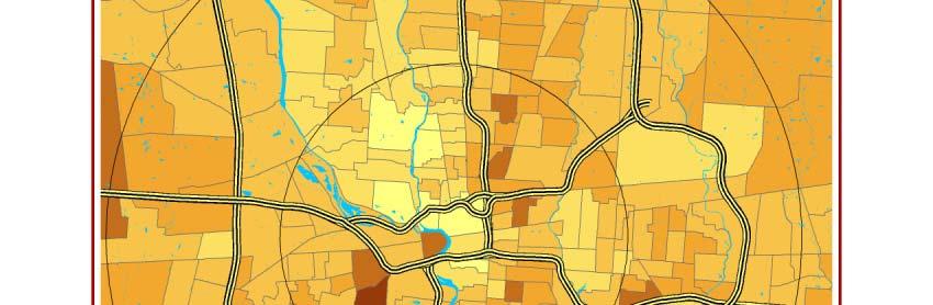
54 Figure 10: Spatial characteristics of Columbus, OH. Rings represent five-mile increments from the city center. Densities and commute times are from the 2000 Census Transportation Planning Package. Land values are from the Franklin County OH Auditor s Office,