Frequent Pattern Finding in Integrated Biological Networks

Transcription

1 University of Tennessee, Knoxville Trace: Tennessee Research and Creative Exchange Doctoral Dissertations Graduate School Frequent Pattern Finding in Integrated Biological Networks Xinxia Peng University of Tennessee - Knoxville Recommended Citation Peng, Xinxia, "Frequent Pattern Finding in Integrated Biological Networks. " PhD diss., University of Tennessee, This Dissertation is brought to you for free and open access by the Graduate School at Trace: Tennessee Research and Creative Exchange. It has been accepted for inclusion in Doctoral Dissertations by an authorized administrator of Trace: Tennessee Research and Creative Exchange. For more information, please contact trace@utk.edu.

2 To the Graduate Council: I am submitting herewith a dissertation written by Xinxia Peng entitled "Frequent Pattern Finding in Integrated Biological Networks." I have examined the final electronic copy of this dissertation for form and content and recommend that it be accepted in partial fulfillment of the requirements for the degree of Doctor of Philosophy, with a major in Life Sciences. We have read this dissertation and recommend its acceptance: Jay R. Snoddy, Arnold M. Saxton, Brynn H. Voy (Original signatures are on file with official student records.) Michael A. Langston, Major Professor Accepted for the Council: Dixie L. Thompson Vice Provost and Dean of the Graduate School

3 To the Graduate Council: I am submitting herewith a dissertation written by Xinxia Peng entitled Frequent Pattern Finding in Integrated Biological Networks. I have examined the final electronic copy of this dissertation for form and content and recommend that it be accepted in partial fulfillment of the requirements for the degree of Doctor of Philosophy, with a major in Life Sciences. Michael A. Langston Major Professor We have read this dissertation and recommend its acceptance: Jay R. Snoddy Arnold M. Saxton Brynn H. Voy Accepted for the Council: Anne Mayhew Vice Chancellor and Dean of Graduate Studies (Original signatures are on file with official student records)

4 Frequent Pattern Finding in Integrated Biological Networks A Dissertation Presented for the Doctor of Philosophy Degree The University of Tennessee, Knoxville Xinxia Peng December 2005

5 Acknowledgements I would like to thank my wife and the rest of my family. Without their support and encouragement, I would not have accomplished so much in my studies. I would like to thank my research advisors, Dr. Michael Langston and Dr. Jay Snoddy, for their valuable mentoring. It was a great experience of studying and working under their guidance. I wish to thank the members of Dr. Snoddy s group and Dr. Langston s group and for the help and discussions. I own a special thank to Adam Tebbe and Suzanne Baktash for their carefully reading and editing this dissertation. I would like to thank my other advisors, Dr. Arnold Saxton, Dr. Brynn Voy and Dr. Frank Larimer for willing to serve on my advisor committee and for their valuable guidance and discussions. I would like to thank the UT-ORNL Graduate School of Genome Science and Technology for providing me the training opportunity. I wish to thank Kay Gardner and Gaynelle Russell for their help. I would like to acknowledge that part of the financial support for my dissertation work came from National Institute of Health. Finally, I would like to take this opportunity to extend my gratitude and regards to all of my teachers. I would like to thank all of the friends that I made in this country. ii

6 Abstract Biomedical research is undergoing a revolution with the advance of high-throughput technologies. A major challenge in the post-genomic era is to understand how genes, proteins and small molecules are organized into signaling pathways and regulatory networks. To simplify the analysis of large complex molecular networks, strategies are sought to break them down into small yet relatively independent network modules, e.g. pathways and protein complexes. In fulfillment of the motivation to find evolutionary origins of network modules, a novel strategy has been developed to uncover duplicated pathways and protein complexes. This search was first formulated into a computational problem which finds frequent patterns in integrated graphs. The whole framework was then successfully implemented as the software package BLUNT, which includes a parallelized version. To evaluate the biological significance of the work, several large datasets were chosen, with each dataset targeting a different biological question. An application of BLUNT was performed on the yeast protein-protein interaction network, which is described. A large number of frequent patterns were discovered and predicted to be duplicated pathways. To explore how these pathways may have diverged since duplication, the differential regulation of duplicated pathways was studied at the transcriptional level, both in terms of time and location. As demonstrated, this algorithm can be used as new data mining tool for large scale biological data in general. It also provides a novel strategy to study the evolution of pathways and protein complexes in a systematic way. Understanding how pathways and protein complexes evolve will greatly benefit the fundamentals of biomedical research. iii

7 Table of Contents Chapter 1.An Introduction to Biological Network Analysis Overview High-Throughput Data Global Features of Biological Networks Local Features of Biological Networks Comparative Network Analysis: Multiple Networks Comparative Network Analysis: Single Network About This Dissertation Chapter 2.Introducing BLUNT: an Instrument for Data Integration and Frequent Pattern Discovery in Molecular Networks Introduction Graph Definitions and Notations Vertex Labeling with Protein Domain Information Graph Comparison Determination of Pattern Frequency Frequent Pattern Finding Algorithm Statistical Significance Assessment Conclusion and Discussion Chapter 3.Finding Frequent Patterns in Protein-Protein Interaction Networks Integrated with Protein Domain Information Introduction Materials and Methods Results Discussion Chapter 4.Detecting Network Motifs in Gene Co-expression Networks through the Integration of Protein Domain Information Introduction Materials and Methods Results Discussion Chapter 5.Differential Expression of Parallel Functional Modules in Mouse Tissues Introduction Materials and Methods Results Discussion Chapter 6.Summary References Appendix Vita iv

8 List of Tables Table 3.1 Total number of network motifs found under different p-values with different domain matching levels (k=3, f=2) Table 3.2 Overview of KEGG pathways and CYGD protein complexes having at least one instance of the predicted network motifs at one of the four protein domain matching levels Table 3.3 The total number of network motifs and associated genes involved in each pathway or complex at each of the four domain matching levels Table 4.1 Summary of the number of putative network motifs detected with different set of parameter values v

9 List of Figures Figure 2.1 The three-kinase cascades in four yeast MAPK signaling pathways Figure 2.2 Graphical view of domain structures of yeast MAPK kinases based on Pfam annotations Figure 2.3 Different ways to match vertices (genes or proteins) in molecular networks based on their corresponding protein domain information Figure 2.4 Different algorithms to match subgraphs to a pattern Figure 2.5 Patterns with the non-monotonic frequency Figure 2.6 Algorithm for frequent pattern finding Figure 2.7 The search space may not be pruned though the frequency of a pattern of intermediate size falls below the frequency of a pattern of target size if algorithms other than graph isomorphism are applied Figure 2.8 The certificates of example subgraphs Figure 3.1 Definition of network motif in protein interaction network Figure 3.2 Overview of p-values of individual frequent patterns detected at Domain Matching Level A Figure 3.3 Overview of p-values of individual frequent patterns detected at Domain Matching Level B Figure 3.4 Overview of p-values of individual patterns detected at Domain Matching Level C Figure 3.5 Overview of p-values of individual patterns detected at Domain Matching Level D Figure 3.6. Histograms of GO similarity scores of instances of network motifs (p < 0.01) Figure 3.7 Different instances of the three-kinase network motif (PF00069, PF00069 and PF00069) detected at domain matching level D were involved in different known pathways/complexes Figure 3.8 Additional examples of network motifs with different instances involved in different pathways or protein complexes Figure 3.9 A schematic diagram of known yeast MAPK signaling pathways superimposed with predicted network motifs detected at domain matching level D Figure 3.10 Another view of 26 proteasome Figure 4.1 Schematic of a network motif in gene co-expression networks Figure 4.2 Degree distributions of co-expression networks generated under different cutoff values of correlation coefficients (R) Figure 4.3 Survey of distributions of Pearson's correlation coefficients for several timeseries gene expression datasets Figure 4.4 Degree distribution of co-expression networks generated under different cutoff values of correlation coefficients (R) when those genes in the Overview Dataset were removed because of their strong periodic behavior Figure 4.5 An example network motif Figure 4.6 Instances found in the yeast protein interaction network for the network motif shown in Figure vi

10 Figure 4.7 Instances of a network motif showing different expression profiles Figure 5.1 Definition of a network motif Figure 5.2 Histogram of GO similarity scores of instances in three datasets: 1) instances of those predicted network motifs with 3 different domain labels (mt, green diamond), 2) 10,000 sets of three randomly chosen proteins from the yeast PPI network (rnd, black circle) and, 3) 10,000 randomly chosen connected subgraphs (cc, red square) from the mouse protein-protein association network in the biological process category Figure 5.3 An example network motif related to the TGF-beta signaling pathway Figure 5.4 Histograms of the number of tissues in which the pairs of instances were differentially expressed Figure 5.5 Node degree distributions are shown for co-expression networks generated under different cutoff values of correlation coefficient (R) Figure 5.6 Keratin related network motif (PF00038, PF00038, PF00038; PF00038: Intermediate filament protein) vii

11 Chapter 1. An Introduction to Biological Network Analysis 1.1 Overview Living systems are composed of thousands of different types of molecules. Wholegenome sequencing efforts have generated comprehensive lists of molecules, genes and proteins. Advances in high-throughput technologies are now enabling researchers to characterize interactions among these molecules systematically. One of the major challenges of post-genomic biology is to understand how interacting genes, proteins and small molecules are organized into modules, especially as pathways and protein complexes. In this chapter, an overview is first given of high-throughput data in Section 1.2. Recent studies on the global and local features of biological networks will be discussed in Sections 1.3 and 1.4, respectively. Sections 1.5 and 1.6 will review the comparative analysis of biological networks. The outline of this dissertation will be presented in Section High-Throughput Data In this section an overview will be given on the available high-throughput data and related techniques including yeast two-hybrid assay, mass-spectrometry based approaches for protein complex identification, microarray technology and synthetic genetic interaction Yeast two-hybrid assay The yeast two-hybrid assay is one of the most widely used methods for the detection of physical protein-protein interactions (Fields et al. 1989). In budding yeast 1

12 Saccharomyces cerevisiae, the GAL4 protein is a transcriptional activator required for the expression of genes encoding enzymes of galactose utilization. It has two domains: the N-terminal DNA-binding domain and the C-terminal activating domain. The yeast twohybrid assay takes advantage of the yeast GAL4 protein by generating a system of two hybrid proteins. A protein X is fused to the DNA-binding domain, while another protein Y is fused to the activating domain of the GAL4 protein. If X and Y form a proteinprotein complex, and bring two GAL4 domains together, the transcription of a GAL4- regulated gene occurs. Using two-hybrid assays, studies have generated several large scale protein-protein interaction data sets in model organisms. Rain et al. (2001) identified over 1,200 interactions in the peptic ulcers pathogen Helicobacter pylori. In S. cerevisiae, two independent studies were carried out to generate a comprehensive list of protein-protein interactions using the two-hybrid assay (Uetz et al. 2000; Ito et al. 2001). There were 957 putative interactions involving 1,004 proteins identified in the first study. In the second study, 4,549 putative interactions found among the 3,278 proteins. The yeast two-hybrid screens were also applied to the metazoan model system. Recently, a two-hybrid-based draft map of 7,048 proteins and 20,405 interactions was generated in fruit fly Drosophilia melanogaster, which was refined to a high confidence map of 4,679 proteins and 4,780 interactions using a computational method (Giot et al. 2003). In worm C. elegans, more than 4,000 interactions were identified from highthroughput yeast two-hybrid screens in 2004 (Li et al. 2004). 2

13 1.2.2 Mass spectrometry-based approaches Mass spectrometry (MS)-based approaches can also be used to identify proteinprotein interactions in a high-throughput fashion. These approaches are particularly effective in detecting protein complexes. Typically, MS-based protein interaction experiments involve three steps: bait presentation, affinity purification of the complex, and analysis of the bound proteins (Aebersold et al. 2003). First, the genes encoding proteins of interests are tagged with a sequence readily recognized by an antibody specific for the tag. These genes are then introduced into live cells. The tagged proteins are expressed. Using the tag, the protein complex with a tagged protein can be pulled out. Those proteins extracted along with the tagged protein are identified using an MS-based method. Two large-scale projects were reported on the yeast protein protein interaction network. In one of the studies, 1,739 TAP-tagged genes were introduced into the yeast genome by homologous recombination. Two hundred thirty two stable complexes were isolated by two sequential steps of affinity purification (Gavin et al. 2002). Proteins in those complexes were identified by matrix assisted laser desorption/ionization (MALDI) peptide mapping after separation by denaturing gel electrophoresis. Another study used transient transfection to express FLAG-tagged bait proteins and single-step immunopurification to isolate protein complexes. In this study, 3,617 associated proteins were identified by automated liquid chromatography (LC)-MS/MS of gel-separated bands (Ho et al. 2002). 3

14 1.2.3 Gene co-expression Large scale gene expression profiling using microarray technology provides a powerful, high-throughput approach to infer relationships among genes. Since genes that encode proteins of the same pathway or the same protein complex are often co-regulated, clusters of genes that are functionally related often exhibit correlated expression patterns under a large number of diverse conditions (Eisen et al. 1998; Hughes et al. 2000; Segal et al. 2003; Stuart et al. 2003). A typical microarray experiment begins with good experimental design. RNAs are extracted from each of the samples collected under different conditions, labeled with fluorescent dyes, and hybridized to microarray slides. The hybridized microarray slides are scanned to acquire the images of the fluorescent probes. Raw expression data for genes is obtained through image analysis. The raw data is then filtered based on quality and normalized. Depending on the aim of the study, different data analyses may be applied. To infer the correlation between a pair of genes, different correlation measures may be used, although the Pearson correlation is one of the most frequently used measures for this (Stuart et al. 2003). In contrast to the mechanisms just described, proteins encoded by correlated genes may not physically interact. For example, the sharing of the same transcriptional factor may result in the co-regulation of two genes, but not necessarily interaction of their protein products Synthetic genetic interaction Synthetic genetic interaction is the other method that can be employed to infer relationships among genes in a large scale. Two genes show a synthetic lethal interaction if the combination of their mutations, neither of which in isolation is lethal, causes cell death (Tong et al. 2001). Synthetic lethal relationships may occur for genes 4

15 acting in a single pathway or for genes within two different pathways if one process functionally compensates for or buffers the defects in the other. Similar to the correlation analysis, the proteins encoded by a synthetic lethal pair may not physically interact. In the yeast S. cerevisiae, less than 20% of the ~6,200 predicted genes are essential, implying that the genome is buffered from the phenotypic consequences of genetic perturbation, possibly because of redundancy (Winzeler et al. 1999). Large-scale synthetic lethal screenings in yeast were carried out by crossing mutations in 132 different query genes into a set of ~4,700 viable yeast gene deletion mutants (Tong et al. 2004). A genetic interaction network containing ~1,000 genes and ~4,000 interactions was mapped in the study. 1.3 Global Features of Biological Networks Although technical advances make data collection ever easier, investigators are increasingly challenged by the need to assimilate the growing mountain of data and to gain view of the bigger picture. Recent advances in network biology indicate that cellular networks are governed by universal laws and offer a new conceptual framework that could potentially revolutionize the view of living systems (Barabasi et al. 2004). One of the basic measures of networks is the connectivity of nodes. The degree of a node is the number of links the node has to other nodes. Here we use link and edge interchangeably. The degree distribution, P(k), is the probability that a selected node has exactly k links. P(k) is obtained by counting the number of nodes N(k) with k = 1, 2 links and dividing by the total number of nodes N. The degree distribution may differentiate networks into classes. 5

16 Many biological networks are proposed to be scale-free, a concept introduced in Barabasi et al. (1999). This means that their degree distribution approximates a power law, P(k) ~ k - γ, where ~ indicates proportional to. γ is the degree exponent, with its value for most networks being between 2 and 3 (Barabasi et al. 2004). Scale-free networks are highly non-uniform, where most of the nodes have low degrees. Only a few nodes have high degrees. These are often called hubs. This is in distinct contrast to the classic random network model, for which the degrees of all nodes are in the vicinity of the average degree. An analysis of the metabolic networks of 43 different organisms from all three domains of life (eukaryotes, bacteria, and archaea) indicates that the cellular metabolic networks are indeed scale-free (Jeong et al. 2000; Wagner et al. 2001). Similar to other real-world networks, biological networks are also small-world networks (Watts et al. 1998; Wagner et al. 2001). This implies that any two nodes can be connected by a path of a few links. Formally, the small-worldness is characterized by two measures: the characteristic path length and clustering coefficient (Watts et al. 1998). Between two nodes there may be multiple different paths. The shortest path is the path with the smallest number of links between them. The characteristic path length L for a network is the average length over the shortest paths between all pairs of nodes. L can be n( n 1) calculated as S( i, j) / i j 2 for a connected graph, where S( i, j) denotes the length of the shortest path between vertices i and j. The clustering coefficient C is defined as follows. For a vertex i with ki neighbors, at most k i (k i 1)/2 edges can exist between them. C i = 2n/k i (k i 1) denotes the fraction of these allowable edges that actually exist. The clustering coefficient C is the average of C i over all i. A small-world network is one 6

17 that is sparse but much more highly clustered than an equally sparse random network (C >> C random ), and its characteristic path length L is close to the theoretical minimum shown by a random network (L L random ) (Watts et al. 1998; Wagner et al. 2001). These global features affect network properties. For example, scale-free networks are resistant to random failure but vulnerable to targeted attack against highly connected hubs (Albert et al. 2000). Deletion analyses indicate that in S. cerevisiae only 21% of the proteins with 5 or fewer interactions are essential, but over 60% for those with more than 15 interactions (Jeong et al. 2001). This indicates that the protein s degree of connectivity has an important role in determining its deletion phenotype. It is worth mentioning that although existing network data is very comprehensive, the coverage of the whole network is still very low. The topological features observed in the incomplete data may not be confidently extrapolated to the complete network. A recent study reported that partial sampling of various non-scale-free networks resulted in subnetworks with topological characteristics similar to those currently available interaction networks, which were considered as scale-free (Han et al. 2005). 1.4 Local Features of Biological Networks The global features give a useful overview of how a biological system works, but it is of limited use to biologists (Bray 2003). Many non-biological networks are also scalefree. These may originate from different mechanisms. To obtain testable biological insights, another direction of network analysis is to decompose large networks into small modules. Alon s group proposed that network motifs are simple building blocks of complex networks (Milo et al. 2002; Shen-Orr et al. 2002). Both biological and non-biological 7

18 networks can be modeled as graphs. A connected subgraph represents a subset of nodes that are connected to each other. The number of distinct subgraphs in a graph tends to grow exponentially with the size of its connected subgraphs. Not all subgraphs occur with equal frequency. Some subgraphs are defined as network motifs, which occur significantly more frequently. To search for network motifs in a given network, all subgraphs of a certain number of nodes in the network are enumerated. Next, the network is randomized while keeping the number of nodes, links and the degree distribution unchanged. Subgraphs that occur significantly more frequently in the real network, as compared to the randomized network, are defined as network motifs. Each network motif is proposed to perform a specific task. For example, feedforward loops (FFLs) were detected in the transcriptional regulation networks both in E. coli and S. cerevisiae, and even in the neural network of C. elegans (Lee et al. 2002; Milo et al. 2002; Shen-Orr et al. 2002). The FFL has three components: a transcription factor X which regulates a second transcription factor Y, and X and Y jointly regulate gene Z. FFLs have eight possible structural configurations, because each of the three transcription interactions can be either positive (activation) or negative (repression). Four of these configurations are coherent : i.e., the sign of the direct regulation path (from X to Z) is the same as the overall sign of the indirect regulation path (from X through Y to Z). Mathematical analysis suggests that FFLs can filter out spurious input fluctuation and allow a rapid system shutdown (Shen-Orr et al. 2002). In an engineered experimental system, the coherent FFL responded rapidly to step-like stimuli of the inducer of X in one direction (ON to OFF), and at a delay to steps in the opposite direction (OFF to ON) (Mangan et al. 2003). 8

19 Computationally, the network motif discovery process is closely related to the frequent pattern finding problem in graph datasets, which has two distinct problem formulations. For the first problem formulation, the input to the pattern finding algorithm is a set of related graphs, which can be relatively small (Inokuchi et al. 2000), or large (Hu et al. 2005). The frequency of a pattern is determined by the number of different graphs in which the pattern occurs, irrespective of how many times a pattern occurs in a particular graph. In the second case, the frequency of a pattern is based on the number of its occurrences in one graph (Kuramochi et al. 2004). The network motif discovery problem falls into the second category. In the case of network motif discovery, the significance of frequent patterns is evaluated by comparison with an ensemble of randomized graphs (Milo et al. 2002), while a typical frequent pattern finding algorithm in a single graph takes a user specified cutoff value for the frequency of patterns (Kuramochi et al. 2004). 1.5 Comparative Network Analysis: Multiple Networks Comparing DNA and protein sequences has been a well-established approach for comparative analysis at the sequence level. The availability of large scale genomic and proteomic data as discussed above opens up possibilities for comparative analysis at other levels, particularly at the level of networks Comparative analysis of known pathways Comparative network analysis can be carried out in at least two different directions. First, the comparative analysis starts with a known pathway or sub-network. The pathway or sub-network of interest may be determined on a well established knowledge basis from literature and experimental data (Dandekar et al. 1999). Homologs of each gene or 9

20 protein in the pathway are identified within the same organism (paralogs) and across different species (orthologs) using sequence alignment. The evolution of the pathway is examined based on the conservation and divergence of individual components of the pathway. Alternative branches or routes may be derived using methods such as algebraic pathway analysis when corresponding orthologs are missing in a genome (Dandekar et al. 1999). In microbial systems, the gene order may also be integrated into defining pathways. This is because functionally related genes are sometimes found within the same operon. (An operon is a cluster of genes located next to each other in bacterial chromosomes that comprises a single transcription unit.) For example, a functionally related enzyme cluster was defined as a set of enzymes which catalyze successive reactions in the metabolic pathway and are also located close together on the chromosome (Ogata et al. 2000). Usually the pathway is represented just as a unique set of genes, but the topology of complex pathways can also be considered in the comparison of pathways. Forst et al. (2001) represented the topology of a metabolic network as an adjacency matrix. The difference between two networks was calculated as the summary of distances on each entry in the adjacency matrices. Paralogs and orthlogs can be scored differently. Gap penalties were introduced to accommodate evolutionary variations and experimental errors (Ogata et al. 2000; Forst et al. 2001) Comparative analysis of high-throughput experimental data To find out how interacting proteins and genes are organized into pathways and protein complexes that provide functionality in the system, the other type of comparative network analysis begins with a pool of datasets collected from different experiments, such as the yeast protein-protein interaction map. The yeast interaction data were 10

21 collected from different experiments, such as thousands of individual yeast two-hybrid assays and affinity purifications as discussed in Section 1.2. Suppose that protein A and B interact under one condition and protein B and C interact under another condition. Proteins A, B and C may be connected as a chain in the pooled dataset, but it is possible that these three proteins never function together. Comparing different networks may help to delineate functional modules like pathways and protein complexes, since many known pathways and protein complexes are conserved across different species. The divergence of living systems may also be revealed by the differences in the patterns of interactions. In contrast to the first approach, this type of analysis generates predictions of pathways and protein complexes, and the results need to be further examined and verified Interologs An underlying assumption of this type of comparative analysis is that interacting proteins in one organism have co-evolved such that their respective orthologs in another organism also interact (Matthews et al. 2001). This notion of conserved interactions was proposed as interologs in Walhout et al. (2000). To investigate the extent to which large-scale searches for interologs may be used for interaction predictions, 257 potential worm interologs were identified from 1,195 two-hybrid yeast interactions (Matthews et al. 2001). A sample of 71 of those worm pairs (corresponding to 72 yeast interactions) was experimentally tested. Of the 72 yeast interactions tested, nineteen (26%) exhibited a detectable interaction. Of these 19 interactions, six (31%) worm pairs were found to interact. In total, 216 worm pairs were experimentally tested and 35 of them (16%) exhibited a detectable interaction. It was suggested that between 16% and 31% was the minimal proportion of true interologs that can be detected between two 11

22 species that are evolutionarily divergent by about 900 million years. This points to between 600- and fold higher frequency of detection of interaction than through conventional two-hybrid screens using random libraries. An average of five interactors per bait typically was obtained using a worm library representing ~19,000 genes (2.6 x 10-4 ) (Matthews et al. 2001). The identification of orthologs is dependent on the cutoff value for the similarity scores from a sequence alignment. Yu et al. (2004) reported that protein-protein interactions could be transferred when a pair of proteins has a joint sequence identity > 80% or a joint E-value < Joint in this context refers to the geometric mean of the sequence identities, or of the E-values for two pairs of interacting proteins. In addition, the concept of conserved regulatory relationship (protein-dna binding) was introduced, and it was suggested to be conserved at thresholds between 30% and 60% sequence identity, depending on the protein family Conservation of interactions at the network level Conservation of interactions between pairs of orthologs suggests that the network of interactions may also be conserved among species. Kelley et al. (2003) proposed a global protein network alignment algorithm to identify conserved pathways. While the term pathway has been broadly used within various biological contexts, in this study a pathway referred specifically to a connected, linear path in the network. The algorithm searched for high-scoring pathway alignment between two paths, one from each of two networks of interest. Proteins in the first path <A, B, C, > were paired against putative homologs that occurred in the same order in the second path <a, b, c, >. When a protein interaction in one path skipped over a protein in the other, a gap was introduced. A mismatch occurred when aligned proteins did not share sequence similarity. Neither 12

23 gaps nor mismatches were allowed to occur consecutively. The algorithm started with a global alignment graph in which each vertex represented a pair of proteins, one from each network. It required that there was at least weak sequence similarity (BLAST E-value 10-2 ) between the pairs of proteins. Each edge represented a conserved interaction, gap, or mismatch. Therefore, a path in the global alignment graph represented an alignment of two paths, one from each network. The scoring of each path was a sum of scores over the vertices and edges of the path, which accounted for similarities in both sequence and interactions. A heuristic iterative algorithm was used to search for high-scoring paths of a specified length. One hundred and fifty highest-scoring pathway alignments of length four were found between protein interaction networks from Helicobacter pylori and S. cerevisiae. In total, it included 4.1% and 1.2% of proteins in the H. pylori and S. cerevisiae proteins in at least one alignment. It should be noted that conservation of direct interaction pairs between two networks was surprisingly rare (7 in total), probably due to low coverage or quality of interactions. A similar approach was also extended to the search for conserved protein complexes between two species by introducing a probabilistic model for protein complexes (Sharan et al. 2004). In the protein-complex model, every two proteins in the complex were assumed to interact with a high probability of some value, which basically is a clique structure. (A clique is a subgraph in which each pair of nodes is connected by an edge.) In the null model, each edge is present with the same probability as it occurs in a random graph. Similarly a global alignment graph was constructed. A likelihood ratio score was used to compare the fit of a sub-network to the clique structure versus the original networks that were randomly constructed. A unified method to detect both paths and 13

24 clusters was proposed and extended to handle more than two species (Sharan et al. 2005). An alignment identified 183 protein clusters and 240 paths (at the significance level of p- value < 0.01) which were conserved across protein interaction networks from C. elegans, D. melanogaster and S. cerevisiae. In total, they covered 649 proteins among three networks, and overlapping clusters were grouped into 71 distinct network regions. These studies provide an important observation for comparative network analysis: within high-scoring alignments, proteins did not necessarily pair with their best sequence matches in another network. For example, 22% (13/59) of yeast proteins were not paired with their best BLAST H. pylori match and 75% (30/40) when bacterial proteins were compared with yeast proteins (Kelley et al. 2003). Out of the 679 protein triplets aligned at the same position with the three-way conserved cluster, only 177 contained at least one of the best sequence matches (Sharan et al. 2005). In the case of the 129 triplets in the conserved paths, only 31 contained best sequence matches. Though it is possible that the best matches were not present in the analyzed networks, these observations also suggest network comparison may provide additional information about the conservation of function Conservation of gene co-expression Similarly comparative analysis can also be used to study the conservation of coexpression (Stuart et al. 2003). Similar to the global alignment graph, a conserved gene co-expression network was constructed. The vertices in the co-expression network were metagenes, analogous to the vertices in the global alignment graph. Each metagene was defined as a set of orthologs across multiple organisms. An orthologous relationship was established if the corresponding protein sequences were one another s best reciprocal 14

25 BLAST hit. An edge was put between two metagenes if the expression of the corresponding genes was significantly correlated in multiple organisms, indicating that their coexpression was conserved across evolution. Four evolutionarily diverse organisms: Homo sapiens, D. melanogaster, C. elegans, and S. cerevisiae were selected because of the extensive availability of microarray data. Twelve network regions of highly interconnected metagenes were identified using a K-means clustering algorithm, and most of them were enriched for metagenes that were involved in similar biological processes (Stuart et al. 2003). 1.6 Comparative Network Analysis: Single Network Finding duplicated pathways by self-against-self alignment of networks from experimental data Homologous features can also be identified within a network. Self-against-self network alignment may reveal paralogous pathways, which are pathways with duplicated proteins and interactions. Using a similar approach as discussed above, the yeast protein interaction network constructed based on experimental data was aligned against itself to obtain 300 highest-scoring pathway alignments of length four (p-value ) (Kelley et al. 2003). To overcome the large size of the potential global alignment graph, vertices were restricted to protein pairs with BLAST E-values 10-10, whereas E-values 10-2 were used for alignment between H. pylori and S. cerevisiae. In addition, no gaps and mismatches were allowed. The tradeoff is that many paralogous pathways would be missed if they diverged enough in sequences or interactions, or both. 15

26 1.6.2 Revealing duplicated pathways through computational predictions from available genomic sequences As an alternative to networks constructed from experimental data, the input network to comparative analysis may be developed from genomic sequences using computational methods. Li et al. (2005) proposed a four-step approach to detect parallel functional modules, a notion analogous to paralogous pathways. Parallel functional modules were believed to be from gene duplication and defined as separate sets of proteins in an organism that catalyze the same or similar reactions. In Step 1, starting from a query genome, all of the possible protein pairs were compared to proteins encoded in 82 other fully sequenced genomes. A binary functional linkage between every pair of proteins was calculated using the Phylogenetic Profile, Rosetta Stone, Gene Neighbor and Gene Cluster methods. A functional linkage can be regarded as an edge in a network. The Phylogentic Profile method identifies co-occurred protein pairs across various genomes, while the Rosetta Stone method identifies protein pairs that fuse into a single peptide in another genome. The Gene Neighbor method identifies the protein pairs residing in close chromosomal proximity in multiple genomes. The Gene Cluster method identifies the protein pairs that are likely to belong to the same operon. The functional linkage was set to 1 if the calculated confidence is above the chosen threshold; otherwise it was 0. In Step 2, a symmetric matrix of functional linkages was constructed. The proteins were clustered based on the similarity of their linkage patterns using a hierarchical clustering algorithm. The rows and columns of the matrix were reordered. Typically clusters showed up on the diagonal of the matrix where proteins in the same pathway or complexes were clustered together. Since a functional linkage does not necessarily mean 16

27 a physical interaction between proteins, these clusters are analogous to the dense gene clusters based on the co-expression. In Step 3, the off-diagonal clusters in the matrix were treated as signatures of parallel functional modules, and identified visually. Off-diagonal clusters consisted of two or more distinct subgroups of proteins. Proteins in the same subgroup usually were not functionally linked to each other. Each subgroup was treated as a collection of the equivalent components in the parallel functional modules, and they were usually paralogous. In Step 4, the corresponding partners from each subgroup were then manually matched. In prokaryotic genomes, the proteins were paired if their genes were located in the same chromosomal region, because these proteins tend to interact with each other within a pathway or complex. For eukaryotic genomes, the proteins were paired based on the closest phylogenetic distances (Gertz et al. 2003; Ramani et al. 2003). The underlying assumption is that proteins that function together evolve at similar rates during evolution. Conceptually, the approach is to superimpose the phylogenetic trees of two protein families. When the approach was applied to ten genomes, thirty-seven cellular systems were identified that had two or more parallel functional modules, the majority (60%) of them were novel (Li et al. 2005). 1.7 About This Dissertation The remainder of this dissertation is organized as follows. Chapter 2 describes the formulation of the biological question into a computable problem. It is followed by the details of the design and implementation of a flexible system, BLUNT, for frequent pattern finding in integrated biological networks. The application of BLUNT on protein- 17

28 protein interaction networks and its biological implications are described in Chapter 3. Chapter 4 describes finding frequent patterns in malaria gene co-expression networks, which are constructed using a large-scale time series gene expression dataset. A particular focus is the temporal differential expression of frequent patterns. Chapter 5 describes finding frequent patterns in the mouse protein-protein association network, and gene co-expression networks constructed from a gene expression data set that profiled a large panel of mouse tissues. The spatial differential expression of frequent patterns is targeted. Chapter 6 summarizes works presented in this dissertation. 18

29 Chapter 2. Introducing BLUNT: an Instrument for Data Integration and Frequent Pattern Discovery in Molecular Networks 2.1 Introduction A major challenge in the post-genomic era is to understand how signaling pathways and regulatory networks are formed by interacting genes, proteins and small molecules. Using high-throughput experimental techniques in biology, such as the yeast two-hybrid assay and mass spectrometry-based protein complex identification, researchers have generated an overwhelming amount of interaction data for diverse organisms. Although those comprehensive interactions maps are still incomplete, and contain a large number of false positives, they provide an opportunity to study networks of interacting molecules. It would greatly simplify the analysis of these large complex networks if they could be broken down into small and relatively independent network modules. Studying network modularity would also provide great biological insights into the basic building principles of complex biological networks. One strategy to dissect large networks into small modules is to search for recurring interacting patterns, or network motifs (Milo et al. 2002). A network is modeled as an unlabeled graph. The numbers of occurrences of all types of n-node subgraphs are counted in the graph as well as in an ensemble of randomized graphs. Network motifs are those subgraphs that occur significantly more frequently in the original graph than in randomized graphs. To integrate additional biological information into studies of network modules, a new strategy is proposed here to search for frequent patterns in molecular networks that 19

30 emerged from the following biological observations. Gene duplication is one of the major factors in the evolution of genome complexity. There is a tendency for interacting proteins to be duplicated together, allowing for the evolution of novel pathways (Fryxell 1996). As a well studied example, mitogen-activated protein kinase (MAPK) pathways represent a set of parallel signal pathways. The core of each of these MAPK pathways is a three-tiered kinase cascade (Widmann et al. 1999) (Figure 2.1). Phylogenetic analysis has suggested that the evolution of new signaling cascades was involved with the coduplication of interacting proteins (Caffrey et al. 1999). More examples of paralogous pathways, which are pathways of duplicated proteins and related interactions, were demonstrated with the development of new computational algorithms based on sequence analysis (Kelley et al. 2003; Li et al. 2005). Although the sequence alignment approach has proven to be tremendously powerful in identifying homologs, multidomain proteins present considerable difficulty. These proteins are especially abundant in eukaryotes (Tatusov et al. 1997; Tatusov et al. 2003). As both the functional and evolutionary units of protein sequences, protein domains present another means for studying protein functions and interactions (Pawson et al. 2003) (Figure 2.2). At the sequence domain level, duplicated pathways and protein complexes may be abstracted as repeated interacting patterns of protein domains and combinations of protein domains. The three-kinase cascades of MAPK pathways, for example, may be represented as occurrences of the pattern with three protein kinase domains connected in a chain (Figure 2.1 and Figure 2.2). In this dissertation, a graph theory-based algorithm is presented to find recurring interacting patterns in molecular networks. Protein domain information is successfully 20

31 Figure 2.1 The three-kinase cascades in four yeast MAPK signaling pathways. 21

32 Figure 2.2 Graphical view of domain structures of yeast MAPK kinases based on Pfam annotations. All kinase proteins have a single kinase domain (green) except Ste11 has an additional SAM domain. 22

33 integrated into the pattern discovery through the labeling of graphs. The reminder of this chapter is organized as follows: Section 2.2 gives related definitions in graph theory and the graph models for two types of biological networks of interest. The integration of domain information through vertex labeling and the specifications of patterns are described in Sections 2.3 and Section 2.4, respectively. Section 2.5 addresses the problem of determination of pattern frequency. The details of the pattern searching algorithm are illustrated in Section 2.6. Section 2.7 addresses the assessment of the statistical significance of putative patterns. The biological applications are discussed in the following chapters. Section 2.8 concludes this study. 2.2 Graph Definitions and Notations A graph G = ( V, E) consists of a set of vertices V and a set of edges E V V. An edge e = ( u, v) connects vertex u and v. Throughout this chapter, it is assumed that the graph is undirected, i.e., there is no direction for the connection between two vertices. The vertices u and v are said to be incident with the edge e and adjacent to each other. A subgraph of the graph G = (V, E) is a graph G = (V, E ) where s s s V s V and E s ( V V s s ) I E. A clique is a subgraph in which every pair of vertices is joined by an edge. The density of a subgraph Gs is 2m/[n(n 1)], where m is the number of edges and n the number of vertices in G s. The sparest subgraph is an independent set. It has no edges. Thus its density is 0.0. The densest subgraph is a clique. It has all possible edges. Thus its density is 1.0. Let us consider labeled graphs. That is, each vertex has a label associated with it. Each vertex of the graph is not required to have a unique label and many vertices may share the same label. The degree of a vertex is the number of 23

34 edges incident with it. Two graphs G = V, ) and G = V, ) are isomorphic if 1 ( 1 E1 2 ( 2 E 2 there is a one-to-one correspondence between their vertices, and there is an edge between two vertices of one graph if and only if there is an edge between the corresponding vertices in the other graph. This dissertation focuses on two types of molecular networks. The first type of molecular network of interest is a protein-protein interaction (PPI) network, which models protein interaction data. In a PPI network, the proteins are vertices (nodes). Two vertices are connected with an edge if the corresponding two proteins interact with each other. The second type of molecular network of interest is a gene co-expression (GCE) network. Usually GCE networks are constructed based on data from microarray experiments. In a GCE network, the genes are vertices, and an edge is put between two vertices if the gene expression levels of two corresponding genes are highly correlated across different conditions. Here gene and protein are used interchangeably to refer to a gene or the product the gene encodes. Let G be the graph modeling the molecular network to be analyzed and G p be a graph representing the pattern of interest. An instance G i is a subgraph of G that matches G p based on the rules of interest. In this work the size of a pattern (subgraph) is defined as the number of vertices in the pattern. 2.3 Vertex Labeling with Protein Domain Information For both PPI and GCE networks, vertices are labeled with the protein domain information annotated on the corresponding proteins (PPI) or the proteins encoded by the corresponding genes (GCE). During the pattern finding process, the matching between 24

35 vertices also requires matching of the related vertex labels, i.e. the protein domain information. Matching of protein domain information between two proteins can be formulated in different ways. To enable researchers to study network modules at different evolutionary distances, a hierarchy of four levels of protein similarities is proposed to match protein domain information with different stringencies. As shown in Figure 2.3, protein domain matching level A requires that two proteins have the same types of domains, the same number of domains of each type, and all domains in the same order in the respective protein sequences from N-terminal to C-terminal. Level A tries to ensure that the two proteins are fully comparable in terms of the domain architecture. Level B requires that two proteins have the same types of domains and the same number of each domain type, but does not consider the order of domains in the respective protein sequences. Level C only requires sharing the same domain types. At this level, the domain duplication and domain shuffling events that occur during evolution are taken into consideration while still ensuring that the basic functions of proteins are comparable. Level D only requires that two proteins share at least one domain. This level is the least restricted, and may help identify the basic common function or ancient function of proteins across vast evolutionary time. As shown in Figure 2.1 and Figure 2.2, the threekinase cascades of both pheromone and starvation signaling pathways would not be found if any of the first three levels is applied. The frequent pattern finding procedure may be run separately using one of the domain matching levels, depending on the researcher s interests. We implement these different levels as follows (Figure 2.3): at the domain matching level A the label for each vertex (protein or gene) is the concatenation of all domain 25

36 Figure 2.3 Different ways to match vertices (genes or proteins) in molecular networks based on their corresponding protein domain information. I. the hierarchy of protein domain matching levels (see Section 3 for detailed description). II. A hypothetical protein P with three domains as listed from N-terminal to C-terminal: α, β and α. III. The vertex labels for P under different domain matching levels: A. αβα: the concatenation of domain symbols in the same order as they locate on the sequence. B. ααβ: the concatenation of sorted domain symbols. C. αβ: the concatenation of different domain symbols in a sorted order. D. P is split into two vertices with labels α and β, respectively. Each of the two vertices connects to the same set of vertices as P does. 26

37 27

38 symbols in the same order as those domains appear in the protein sequence. The label is the concatenation of all domain symbols in a sorted order at the domain matching level B. For domain matching level C, the label is a concatenation of all unique domain symbols in a sorted order. At domain matching level D, each protein is split into the same number of new proteins as the number of different domains it has. Each new protein inherits one of the different domains, and all connections from the original protein. Each of these new proteins is modeled as a vertex in the graph. These vertices each now have a label for just one protein domain. One of the advantages of the implementation of Level D is that alternative splicing is accounted for at different protein domain matching levels, which is especially widespread in mammalian genomes (Thanaraj et al. 2004). Due to alternative splicing, one gene may encode multiple proteins and some of these proteins may have different domain information. Typically, available biological data centers around genes and the actual protein variants involved are unknown. To accommodate this limitation, it is assumed that each of the protein variants interacts with the same set of vertices (proteins or genes). A vertex is created for each of these protein variants of the same gene and each of them connect to the same set of vertices as the original gene does. The gene itself is removed and then those vertices are labeled with their protein domain information in the same way as described before. If some protein variants from the same gene have the same label, only one of them is kept and the rest are removed. Since the same gene may be represented multiple times in the labeled graph, it is required that each gene can only appear at most once in each subgraph studied. More details are described in Section 2.6. The disadvantage is that the graph size increases 28

39 when many vertices are split into multiple vertices using the current labeling algorithm, since it increases the graph size, and therefore the computational time and memory requirements as well. 2.4 Graph Comparison Matching subgraphs with different stringencies As described in the Section 2.2, a pattern is a subgraph that occurs many times in a given graph. To find the occurrences of a pattern in a given graph, one can enumerate all of those subgraphs of the same size as that of the pattern, and then compare these subgraphs to the pattern one by one. If a subgraph matches the pattern, the frequency of the pattern increases by one. In the existing literature, the match between a subgraph and the pattern is based on graph isomorphism, which requires the exact matching of both vertices and edges in the two graphs (Figure 2.4). This stringent requirement might not be appropriate as discussed below and alternatives should be provided to meet different needs. One of the primary concerns is the high level of noise in currently available biological data. More than 50% of the high-throughput interaction data was estimated to be false positives as reported in a recent study (von Mering et al. 2002). In addition, the majority of interactions in an organism are still unknown, even for the well-studied yeast organism (von Mering et al. 2002). A subgraph which would match the pattern perfectly could be missed if one interaction was missing or one false interaction occurred in the experimental data. A second consideration is the gamut of biological variation. Similar to biological sequences, two perfectly matched pathways or protein complexes would have divergent 29

40 Figure 2.4 Different algorithms to match subgraphs to a pattern. I. G p is a pattern of interest in a PPI network that has 4 edges connecting 4 vertices (proteins). The vertices are shaded to indicate their vertex labels. Correspondences between shadings and vertex labels are shown in IV. 1. When graph isomorphism is applied subgraph G s1 matches to G p. 2. Subgraph G s2 also matches to G p based on subgraph isomorphism. 3. When only the combinations of vertex labels are considered, subgraph G s3 matches to G p too. Because they have the same combination of vertex labels: (αβ, β, γ, θγ). Note: a vertex label can be a combination of two or more domains. For example, αβ represents that two domains α and β are on a protein. II. G c is a complete subgraph, i.e. a clique, in a GCE network. All of the subgraphs in I can match to G c if graph isomorphism is not chosen. III. A clique in GCE networks. The vertices in the clique are labeled with cis-regulatory elements (CREs) annotated on their corresponding genes. The clique represents a set of genes which are tightly co-regulated by a common set of cis-regulators, since all of the genes have the same CRE labels. 30

41 31

42 patterns of interactions during evolution. Previous studies have tried to accommodate these evolutionary variations and experimental errors in the network by allowing gaps and mismatches or similar measurements (Kelley et al. 2003; Li et al. 2005). Subgraph isomorphism is more suitable for this type of analysis than graph isomorphism. A match is declared if a subgraph is isomorphic to a subgraph of the pattern. In doing so, the investigator insures that the subgraph is similar to the pattern, but does not require exactly the same topology as the pattern of interest. Therefore, some variations in the interactions are allowed for subgraph matches, but the overall interaction pattern is bounded by the pattern. Still, one of the remaining difficulties is the presence of false positive interactions. A perfectly matched subgraph would be missed because of one false interaction. One could take the opposite side of subgraph isomorphism at the same time by also considering it a match if the pattern is isomorphic to a subgraph of the subgraph of interest. Under this approach, the topology of the subgraph is unbounded by the pattern in some sense. Therefore, it was decided to take the analysis further to connected subgraphs with the same combination of vertex labels. A match is produced if a connected subgraph has the same combination of vertex labels as the pattern does (Figure 2.4). Essentially the topology of the subgraph is ignored except the requirement that the subgraph has to be a connected subgraph. This will determine the upper bound of the number of subgraphs in the graph that could match to the pattern. This approach also offers a convenient way to compare subgraphs between PPI and GCE networks as described below. 32

43 In summary, to match subgraphs to patterns of interest three ways are provided in BLUNT in general. These are graph isomorphism, subgraph isomorphism and connected subgraph with same vertex labels Special considerations for GCE networks Special considerations should be given to subgraphs in GCE networks. Each edge in a GCE network indicates that two genes connected by the edge are highly correlated. Based on the assumption that functionally related genes are highly correlated, biologically meaningful subgraphs often are those densely connected subgraphs (Hu et al. 2005), although the exact interaction information among genes is unavailable under these situations in general. Since the appropriate density is a parameter that needs to be fine tuned in different studies, it is decided to simplify the issue of choosing this parameter by focusing on the densest subgraphs. The densest subgraphs in a graph are cliques, in which each vertex connects to every other vertex (Figure 2.4). When searching for patterns in the GCE network, only cliques are considered. Both patterns and occurrences of patterns are cliques. Often, it is desirable to compare results from GCE networks with subgraphs in PPI networks, or vice versa. A clique in a GCE network represents a set of highly correlated genes. To find out if genes in the clique are part of a pathway or protein complex, the clique may be compared to subgraphs in a PPI network. Ideally, the objective is to find out if proteins encoded by the same set of genes form a subgraph in the PPI network. It will be sufficient to confirm that those genes are indeed functionally related as long as proteins encoded by them form a connected graph. The interactions among those proteins will provide extremely valuable detailed information about relationships among those 33

44 proteins and genes. In practice though, the protein interaction information is unlikely to available in general. It is still informative to know if proteins encoded by their homologs or proteins with similar protein domains interact. In summary, the natural way to compare results from GCE networks with subgraphs in PPI networks is to find connected subgraphs of the same combinations of vertex labels in PPI networks (Figure 2.4). This type of comparison would provide insights into how these genes and their protein products in each clique interact, and if those interactions are conserved Integration of cis-regulatory elements Another interesting biological question concerns cis-regulators in GCE networks. The challenge is to determine if the genes in a densely connected subgraph are regulated by one cis-regulator such as a transcription factor or a common set of cis-regulators. This question can be indirectly addressed by examining cis-regulatory elements (CREs) associated with each gene. Therefore genes in GCE networks can be labeled with corresponding CRE information, instead of protein domain information. The framework laid down in this and the previous sections can be equally applied to address this question (Figure 2.4). Therefore, in this study the investigator chooses to provide a spectrum of strategies to match subgraphs to patterns of interests. It includes graph isomorphism, subgraph isomorphism, connected subgraph and clique. The flexibility of this design enables researchers to choose different approaches depending on their own needs. 2.5 Determination of Pattern Frequency The frequency of a pattern in a graph of interest is the maximum number of different subgraphs matched to the pattern. These subgraphs are called matches of the pattern in 34

45 the given graph. Depending on which elements of the graph can be shared by two matches the frequency of a pattern may be determined differently. Two matches may share the same vertices or edges. As motivated by the concept of paralogous pathways resulting from gene duplication, two matches are defined as overlapping if they share one or more vertices, instead of edges. Two non-overlapping matches have no common vertex. This is more restrictive than the concept of overlapping based on edge-sharing (Kuramochi et al. 2004). In PPI networks, the non-overlapping subgraphs may be viewed as completely duplicated pathways, and in GCE networks they can be viewed as nonoverlapping clusters of genes Counting overlapping subgraph matches Biologically, it can be argued that overlapping matches are equally as important as non-overlapping ones, because the same genes or proteins can function differently along with different partners. As shown in Figure 2.1, the three-kinase cascades in pheromone and starvation pathways share two out of three kinases. This approach, however, presents a computational challenge by allowing arbitrary overlaps between subgraphs matched to the same pattern as described in Kuramochi et al. (2004). The resulting frequency is no longer downward closed. That is, the frequency of a pattern does not vary inversely with its size (Figure 2.5). The outputs can be overwhelmingly large, and this may make the follow-up analyses extremely difficult. On the other hand, the frequency of the pattern could be determined by counting the maximum number of non-overlapping subgraph matches of the pattern, and then the resulting frequency is downward closed. In doing this though, many biologically meaningful subgraph matches will be missed. To balance the biological significance and the computational challenge, a parameter f is set 35

46 Figure 2.5 Patterns with the non-monotonic frequency. A: the graph of 10 vertices. B: a pattern of 4 vertices. C: a pattern of 5 vertices. Using graph isomorphism, only one subgraph of the graph in A can match to the pattern in B, but there are 6 different subgraphs which can match to the pattern in C. up to filter the list of outputs, where f is defined as the minimum number of nonoverlapping matches of a pattern. Only those patterns with at least an f minimum number of non-overlapping matches are output for the follow-up analyses. Unfortunately, quite often this problem can be intractable. It involves solving the maximum independent set problem (MIS) to decide if a pattern has at least f nonoverlapping matches. The MIS problem is a dual to the clique problem, which is NPcomplete. But from the biology point of view, too many interesting patterns could be missed if a large value is set for the parameter f. Often it makes sense to choose the value 2 for the parameter f, as it may be seen that the pathway has been completely duplicated at least once. During evolution, there may be many partial duplication events of a pathway before complete duplication of the pathway occurs. Furthermore, the significance of each pattern will be evaluated by the comparison to an ensemble of randomized graphs after passing this filter as described in Section 2.7. An insignificant 36

47 pattern will be filtered out, even though it may have a large number of non-overlapping matches A special feature for GCE networks In addition, another feature is calculated for the set of matches of a pattern in a given graph, namely, whether the vertices of these subgraph matches form two or more connected components. This is specially designed to target subgraph matches in GCE networks, though it is an interesting feature by itself. As described above in GCE networks, all subgraph matches of a pattern are cliques. If the vertices of those cliques in a graph form at least two connected components, then there is no edge between at least two sets of cliques. Therefore, genes that belong to at least two cliques, each being from a connected component are differentially expressed, while genes within each clique are highly correlated. This implies that genes within each clique may form a functional module, such as a pathway. These functional modules represented by cliques may have similar functions because of the similarity in protein domain information, but they function under different conditions. In this sense, the proposed approach can be used to detect alternative pathways or protein complexes. It may also suggest that duplicated pathways have diverged at least at the transcriptional level. Further analysis of these genes may help shed light on the evolution of pathways. In BLUNT, this feature is set as a parameter. Through this parameter, users can subset patterns to those for which the vertices of their subgraph matches form two or more connected components. 2.6 Frequent Pattern Finding Algorithm In order to find patterns with a significantly higher frequency of occurrence in a graph, one can: 1) enumerate all of its subgraphs of a given size, 2) count the occurrences of 37

48 each pattern by matching each subgraph to the pattern and 3) compare their frequencies with those in an ensemble of randomized graphs. An overview of the algorithm for finding frequent patterns is given in Figure 2.6. The downward closure property allows the pruning of the search space when graph isomorphism is used to match subgraphs to a pattern, but this is not true when other algorithms are applied (Figure 2.7). To accommodate the needs of different algorithms of graph comparisons as described above, a certificate is computed for each subgraph and stored for all subgraphs in a binary search tree (Figure 2.8). The certificate of a subgraph includes three parts: 1) the number of vertices in the subgraph, 2) the labels of the vertices in the sorted order and 3) the degrees of the vertices. The degrees in the last part are partitioned into blocks based on vertex labels. Degrees of vertices with the same label form a block. The degrees within each block are in a sorted order. The last part is computed only when graph isomorphism is used. If a subgraph matches the pattern, it must have the same certificate as the pattern. This provides a way to prune the search space for each pattern. In the binary search tree, subgraphs are indexed by their certificates and stored in the linked list attached to the corresponding node. Essentially, subgraphs are sorted into relative homogenous groups before any graph comparison algorithm is further applied. A simple approach to enumerate all subgraphs in a graph is to create a subgraph of single vertex in the original graph, recursively add neighboring vertices until the subgraph reaches the desired size, then repeat the same procedure for every other vertex in the original graph. This method will repeatedly generate the same subgraph multiple times, since there are many paths to the creation of each subgraph, and each will be 38

49 Figure 2.6 Algorithm for frequent pattern finding. 39

50 Figure 2.7 The search space may not be pruned though the frequency of a pattern of intermediate size falls below the frequency of a pattern of target size if algorithms other than graph isomorphism are applied. A. a graph has 12 vertices. B. The pattern of size 4 has 3 subgraph matches in the graph. C. All of the patterns of size 3 only have 2 subgraphs in the graph. When the value of f parameter is set to 3, the pattern as shown in B will be missed if the search space is pruned at the level of pattern of size 3. 40

51 Figure 2.8 The certificates of example subgraphs. The certificate is on the right side of each of the corresponding subgraphs. Each certificate has three parts as indicated by solid vertical lines: 1) the number of vertices in the subgraph (4 for all subgraphs in this example), 2) the vertex labels in a sorted order and 3) the degrees of the vertices that are first partitioned based on vertex labels (indicated by the dashed vertical lines) and then sorted. θ' is a concatenation of two labels: θ and γ. 41

52 explored. An efficient algorithm is implemented as described in White et al. (2001) such that each subgraph is enumerated exactly once. In the case of clique enumeration in GCE networks, all subgraphs are subject to clique testing before expansion. When graph or subgraph isomorphism is specified for matching subgraphs to a pattern, the list of subgraphs of the same certificate will be further partitioned into several small groups (line 4 of subroutine refine in algorithm 1). In the case of graph isomorphism, within the same group each subgraph is isomorphic to every other and no subgraph is isomorphic to a subgraph from any other group. For each group of subgraphs, the pattern can be represented by any one of them. When subgraph isomorphism is applied, the pattern is represented by the first subgraph within each group and every other subgraph is isomorphic to a subgraph of the pattern. One subgraph may occur in multiple groups, but there will be no subgraph isomorphism between the first subgraphs from each of any two groups. It is a difficult computational problem to test the subgraph and graph isomorphism since they are NP-complete. The mostly commonly used algorithm, Ullmann s, is implemented (Ullmann 1976). The same algorithm is employed to test both graph and subgraph isomorphism. Testing if a pattern has at least f non-overlapping instances involves another NP-complete problem. An algorithm using exhaustive searching along with some preprocessing is implemented, since it is expected the value for f will be small for current applications (2 or 3 in general). 2.7 Statistical Significance Assessment Unlike some studies (Kuramochi et al. 2004), here the discovered frequent patterns are subject to further testing of statistical significance. Because of the different abundances of protein domains and connection densities of proteins and genes, some 42

53 patterns may occur multiple times by chance. Recent studies have shown that real world networks have different characteristics than classical random graph models, such as scale-free degree distribution (Jeong et al. 2001; Lee et al. 2004). The statistical significance of each pattern is assessed by comparisons to randomized graphs generated with the following four algorithms. Starting from the original graph with labeled vertices, a randomized graph is generated by: 1.) randomly permuting the labels of all vertices while leaving the connections in the graph untouched or 2.) randomly permuting the degrees of all vertices and re-connecting all vertices based on assigned degrees by permutations, while keeping vertex labels unchanged (Newman et al. 2001) or 3.) disconnecting all connections and randomly re-connecting all vertices based on their original degrees, to keep all vertices with the same degrees and vertex labels (Newman et al. 2001) or 4.) randomly switching partners between two pairs of connected vertices (Maslov et al. 2002). The frequent pattern finding procedure is then run on the resulting randomized graph. This process was repeated multiple times. The fraction of times the same pattern with the same frequency or higher is found in randomized graphs gives a p-value. The maximum p-value from the four methods is defined as the final p-value of the pattern. In contrast to the de novo discovery of frequent patterns, as discussed in the last section, patterns are already known here. Therefore the subgraph enumeration procedure as described above is modified here to ensure that only those subgraphs which will have 43

54 the same combination of vertex labels as the pattern of interest are expanded. This reduces the computational time significantly. Even so, this step is still computationally intensive, because the simulation has to be repeated many times (typically 10,000 times), to get a very reliable assessment. At the same time, the simulation procedure is highly parallelizable, therefore two different parallel versions of this procedure are implemented using Message Passing Interface (MPI, and both are implemented in master-slave mode. In the first version, the master process distributes equal number of simulations plus seeds for the random number generator to each slave process, including itself. Every process runs independently and sends results back to the master process. In the second version, the master process divides the total number of simulations into many small blocks of jobs first. When a slave process sends back results for previously assigned jobs, the master process receives this, and sends a new block of jobs to the slave process. This repeats until all jobs are finished. The first version is static, and more suitable for a dedicated computer cluster. The second one is dynamic, and better when the workload on each machine varies along with time. For example, this could happen in a cluster open to the public. But the second implementation may increase the computational time because of the increased amount of communication that is required. 2.8 Conclusion and Discussion Based on the theory of evolution, the investigator has carefully designed a framework to integrate multiple sources of data, and then mine large scale complex biological data. Recognizing the complexity of both the theoretical biological questions and the practically available data has enabled the researcher to design a software package, 44

55 BLUNT, with a great flexibility. The implementation with different parameters was designed to meet the diverse needs of the scientific community. Successful applications of the system on various real world biological datasets are demonstrated in the following three chapters. Although the strength of this system has been proved in the following chapters, still there are several ways in which it may be improved in the future. One of remaining challenges is that there can be a large number of subgraph matches to a pattern, which is partially due to the fact that those subgraphs are allowed to be highly overlapping with each other. It is biologically meaningful to do so, as shown in real biological examples, although technically it becomes difficult for the following analysis. In addition, many of those subgraph matches may be false positives for at least two reasons. First, many of the interactions are false positives as discussed above. With the improvement of experimental techniques and the development of new computational algorithms, the input data will become more accurate. Second, protein interaction data is static, but not all of the proteins present and interact at a single time and location, as modeled in a graph (Luscombe et al. 2004). So, the predictions based on the analysis of static interaction data, as shown here and elsewhere, need to be further evaluated. One possible approach is to integrate other types of data. For example, it may be helpful to study the expression of corresponding genes in subgraph matches of a pattern, since rich microarray data is readily available now, and much more gene expression data is expected to be available in the future. The rationale is that functionally related genes tend to be co-expressed, or at least their transcripts tend to co-exist. Another approach is to compare the results from 45

56 data across different species. The true functional modules may tend to be conserved, which may even tell how biological networks evolve. This system involves several NP-hard problems. One particular limitation of the current implementation is subgraph enumeration. The total number of possible subgraphs will increase exponentially with the increase of subgraph size. It puts a tremendous burden on the computational resources required, especially in terms of the memory requirement. While current implementation is designed to focus on small patterns, more research on the algorithm side is needed to explore larger patterns. At the same time, it is also helpful to port the system to supercomputers with a large resource of shared memory. In summary, to meet the needs of systems biology, a new computational framework is designed and implemented. Preliminary application on real biological data provides great insight into the building principles of molecular networks. However, more research is still needed to improve the current system in the future. 46

57 Chapter 3. Finding Frequent Patterns in Protein-Protein Interaction Networks Integrated with Protein Domain Information 3.1 Introduction Proteins do not function alone. Using high-throughput experimental techniques, such as the yeast two-hybrid assay and the mass spectrometry based protein complex identification method, researchers have generated an overwhelming amount of interaction data for diverse organisms. Comprehensive interactions maps, though still incomplete and abundant with false positives, provide an opportunity to study networks of interacting molecules. One of the major challenges is to understand how these interacting genes, proteins and small molecules are organized into functional modules, especially pathways and protein complexes. Based on the theory of genome evolution, different strategies have been proposed to predict duplicated pathways and protein complexes. Gene duplication is one of the major factors in the evolution of genome complexity. There is a tendency for interacting proteins to be duplicated together, allowing for the evolution of novel pathways (Fryxell 1996). As a well studied example, mitogen-activated protein kinase (MAPK) pathways represent a set of parallel signal pathways, and the core of each of these MAPK pathways is a three-tiered kinase cascade (Widmann et al. 1999). Phylogenetic analysis has suggested that the evolution of new signaling cascades have been involved with the coduplication of interacting proteins (Caffrey et al. 1999). More examples of paralogous pathways, or pathways of duplicated proteins and related interactions, have been 47

58 demonstrated with the development of new computational algorithms based on sequence analysis (Kelley et al. 2003; Li et al. 2005). Although the approach of sequence alignment has proven to be tremendously powerful in identifying homologs, multidomain proteins present considerable difficulty. These proteins are especially abundant in eukaryotes (Tatusov et al. 1997; Tatusov et al. 2003). As both the functional and evolutionary units of protein sequences, protein domains present another means for studying protein functions and interactions (Pawson et al. 2003). At the sequence domain level, duplicated pathways or protein complexes may be abstracted as repeated interacting patterns of protein domains. The three-kinase cascades of MAPK pathways, for example, may be treated as multiple occurrences of a pattern with three protein kinase domains connected in a chain. In other words, duplicated pathways may be detected through searching for correlated sequence signatures, and sequence domains will be the natural choice for representing those sequence signatures. Several statistical methods have been developed to detect significantly correlated pairs of protein domains, and those correlated domain pairs were used to predict protein interactions (Sprinzak et al. 2001; Deng et al. 2002; Ng et al. 2003; Nye et al. 2005). But it remains unclear if three or more domains tend to co-occur in some cases and what those domains are, and how they interact if this indeed happens. The generalized form of correlated domain analysis with an arbitrary number of domains is the frequent subgraph pattern finding problem (Kuramochi et al. 2004). To search for frequent interacting patterns with statistical significances in networks, the concept of network motifs was proposed (Milo et al. 2002). Similarly, using a network motif-based strategy, a recent work reported that there were only a few basic interaction 48

59 patterns in protein interaction networks when integrated with structural domain interaction data (Moon et al. 2005). The most dominant network motif was the intermolecular domain interaction, that is, two different interacting domains D1 and D2 belong to different protein chains P1 and P2. Since corresponding protein domains in individual occurrences of the same network motif may differ, correlated domains were not studied. As motivated by the network motif-based strategy, a novel integrated approach is proposed to predict modules of pathways and protein complexes and applied to a comprehensive yeast protein interaction dataset. Through introducing a hierarchy of protein similarities, protein domain information is successfully integrated into the network motif discovery process. The biological relevance of detected network motifs is evaluated by available information from different sources, such as Gene Ontology annotations, known pathways and protein complexes. Novel insights into the organization of molecular networks are revealed. 3.2 Materials and Methods Protein interaction network In the graph of a Protein-Protein Interaction (PPI) network, proteins are represented by nodes (vertices). An unweighted and undirected edge is placed between two nodes if there are documented interactions between the corresponding proteins. The budding yeast S. cerevisiae protein-protein interaction data and associated protein sequences were downloaded from the Database of Interacting Proteins (DIP) (Salwinski et al. 2004) as of July 2004, which contains a total of 4,773 proteins with 15,461 interactions among them. These interactions represented a pooled collection of datasets derived from different 49

60 experimental approaches, including several high-throughput studies using two-hybrid or pull-down methods. Interactions were removed if they involved proteins whose DIP identifiers could not be converted into SGD identifiers ( After the removal of self-self interactions, 4,731 proteins and 15,112 interactions remained. Yeast proteins were annotated with Pfam domains ( Release 14.0, 7,459 Pfam-A domain families) by running HMMER ( locally with trusted cutoffs according to Pfam. Proteins were removed if they did not have any Pfam domain annotations or became isolated after removing proteins without Pfam annotations. The final yeast PPI network contained 2825 proteins and 8736 interactions Network motif definition The concept of network motifs was proposed by Alon s group in studying various real world networks, including biological networks (Milo et al. 2002; Shen-Orr et al. 2002). Here, the concept of a network motif was extended to labeled graphs (Figure 3.1). Specifically, a network motif is defined as a recurring pattern of interacting domain information in a PPI network, in which proteins are labeled with their protein domain information. Each occurrence, or instance of a network motif is a subgraph in the network. Biologically, a network motif may be regarded as an ancient pathway or protein complex, and each occurrence or instance is a copy of that. In general, all instances of a network motif are isomorphic to the pattern (graph isomorphism problem (Garey et al. 1979)), which requires the exact matching of both vertices and edges between an instance 50

61 A. Network Motif {,, } Protein domain α Protein domain β and γ Protein domain θ B. Instances in Protein-Protein Association Network Protein 1 Protein 4 Protein 7 Protein 2 Protein 3 Protein 5 Protein 6 Protein 6 Protein 8 I II III Figure 3.1 Definition of network motif in protein interaction network. (A) A network motif is a combination of domain information. (B) Occurrences or instances of the network motif in a protein-protein interaction network. For each instance, protein domain information of proteins can map one-to-one to the specified network motif. Instances II and III are "overlapping. On the other hand, instance I does not share any proteins with instance II, and are "non-overlapping. 51

62 and a pattern. As discussed below, it is argued that this requirement is not appropriate in this study, and an alternative definition is proposed. The first consideration is evolutionary variation. Similar to biological sequences, two duplicated copies of an ancient pathway or protein complex would also diverge in the patterns of interactions during evolution. The second consideration is the high level of noise in currently available experimental data. More than 50% of the high-throughput interaction data has been estimated to be false positives as reported in a study (von Mering et al. 2002). In addition, the majority of interactions in an organism are still unknown, even for the well studied organism yeast (von Mering et al. 2002). A subgraph that matches perfectly to the pattern could be missed if one interaction was missing, or one false interaction occurred in the experimental data. Third, a significant amount of protein interaction data was from mass spectrometry-based protein complex identification experiments. The internal topology of protein complexes is typically not available. Depending upon the models used, the topology of the protein interaction network may differ significantly (Bader et al. 2002). Previous studies have already attempted to accommodate these evolutionary variations and experimental errors in network data by allowing gaps and mismatches or similar measurements (Kelley et al. 2003; Li et al. 2005). It was decided to take this kind of analysis further to connected subgraphs with the same combination of vertex labels. It considers a connected subgraph as a match to a pattern, or an instance of the pattern if the subgraph has the same combination of vertex labels as the pattern does (Figure 3.1). Essentially the topology of the subgraph is ignored except requiring that it be a connected subgraph. This will also give the upper bound of the number of subgraphs 52

63 in a given graph which could possibly match to the pattern. This definition may be treated as generalized domain correlation analysis, which goes beyond pairs of domains (Sprinzak et al. 2001; Deng et al. 2002; Ng et al. 2003; Nye et al. 2005). More discussion is covered in subsection Two instances are overlapping if they share at least one vertex (protein), otherwise they are non-overlapping. Parameter f is defined as the minimum number of non-overlapping instances, and the number of proteins within each instance, k, as the size of a network motif. We labeled proteins in the yeast PPI network with their Pfam domain annotations and enumerated all connected subgraphs of size k in the graph. Each subgraph is associated with a certificate: a set of string labels (D 1, D 2,..., D i,..., D k ) in a sorted order where each D i is the domain information annotated on the corresponding protein i. Subgraphs were then grouped based on common certificates. The common set of string labels shared by a group of subgraphs was a putative network motif. The number of subgraphs in each group is the number of occurrences or instances of the putative network motif. Next, the parameter f was used to trim the list of putative network motifs. Only the putative network motifs having at least f non-overlapping instances were kept for the following analysis Statistical significance assessment Because of the different abundances of protein domains and different connection densities of proteins, some combinations of protein domain labels may occur multiple times by chance. The statistical significance of each network motif was assessed by comparisons to randomized networks generated with the following four algorithms. Starting from the real PPI network with nodes labeled with protein domain information, a 53

64 randomized network was generated by: 1) randomly permuting the domain labels of all nodes, while leaving the connection structure of the graph untouched, or 2) randomly permuting the degrees of all nodes and re-connecting all nodes based on corresponding permutated degrees, while keeping the same domain labels (Newman et al. 2001), or 3) disconnecting all connections and randomly re-connecting all nodes based on their original degrees to keep all nodes with the same degrees and domain labels (Newman et al. 2001), or 4) randomly switching partners between two pairs of connected nodes (Maslov et al. 2002). The network motif detection procedure was then run on the resulting randomized network. This process was repeated 10,000 times. The fraction of times the same network motif with the same number of instances or more was found in the randomized networks gave a p-value. The maximum p-value of the four methods was defined as the p-value of the network motif Protein similarity hierarchy A protein may have multiple domains. Matching of protein domain information between two proteins can be formulated in different ways. A hierarchy of four levels of protein similarities is proposed to match protein domain information with different stringencies. Protein domain matching level A requires that two proteins have the same types of domains, the same number of domains of each type, and all domains in the same order in the respective protein sequences from N- to C-terminal. Level A tries to ensure that the two proteins are fully comparable in terms of the domain architecture. Level B requires that two proteins have the same types of domains and the same number of each domain type, but does not consider the order of domains in the respective protein sequences. Level C only requires sharing the same domain types. At this level, the 54

65 domain duplication and domain shuffling during evolution are taken into consideration, while still ensuring that the basic functions of proteins are comparable. Level D only requires two proteins share at least one domain. This level is the least restricted, and may help identify the basic common function or ancient function of proteins across deep evolutionary time. While in previous correlated domain pair studies the correlation was studied only between pairs of single domain, the correlation between two combinations of multiple domains may also be studied here, depending on the specified domain matching level. If all proteins have one domain, all domain matching levels will be the same. This offers an opportunity to study pathways and protein complexes at different evolutionary distances. To demonstrate the differences among four domain matching levels, the network motif detection procedure was run separately using each one of them Gene Ontology similarity Similarities between pairs of Gene Ontology (GO) terms were calculated using the similar information-theoretic approach (Wang et al. 2004). Briefly, let C denote the set of GO terms annotated to all proteins in the network being analyzed, plus all of their parent terms. For each GO term c, c C, p(c) is the probability of finding a gene/protein annotated with a child of c inc. For a given c and c, the similarity score was calculated as: i j sim( c, c i j 2 max [ log( p( c))] c S ( ci, c j ) ) = log( p( c )) log( p( c )) i j (1) S c i, c ) is the set of parent terms shared by both c and c, max represents the ( j maximum operator, and sim c i, c ) varies between 0 and 1. ( j i j 55

66 A protein can be multifunctional, thus annotated with several GO terms. A set of proteins may be functionally related under only one condition, thus share a single GO term or a set of closely related GO terms, depending on available information. To evaluate if a set of proteins are functionally related based on similar GO annotations, the GO similarity score for a set of proteins was defined as the maximum average similarities among terms annotated to each protein (one term per protein), and their lowest common ancestor (LCA) term. For example, for a set of three proteins p, p and p, the similarity score may be calculated as: i j k SIM ( p, p c A, c l i m i j, p max ) = A, c A, c S ( c, c j n k k l m, c n ) [ sim( cl, c) + sim( c 3 m, c) + sim( c n, c)] (2) where proteins p, p and p were annotated with sets of terms A, A and A, and i j k i j k S( cl, cm, cn ) is the set of common ancestor terms shared by c, c and c. Thus a higher l m n similarity score implies proteins within the set of proteins tend to have more similar GO annotations. GO annotations of yeast genes were downloaded from SGD (Dolinski 2004). 3.3 Results Prediction of network motifs Considering the incompleteness of yeast protein interaction data and inspired by cascades of three kinases in the MAPK pathways (Widmann et al. 1999), it was decided to search for small network motifs and set k, the size of network motif, to be 3. Also the minimum non-overlapping instances f was set to 2, to carry out a comprehensive search at all four different domain matching levels. Table 3.1 shows a summary of the numbers of network motifs found. For all four domain matching levels, the first two graph 56

67 Table 3.1 Total number of network motifs found under different p-values with different domain matching levels (k=3, f=2) Protein domain matchin g level Total number of putative network motifs Number of network motifs with p- value less than Number of network motifs with number of different domain labels equal to (pvalue < 0.01) A B C D randomization methods gave very similar results. The last two methods also gave similar results, but they were more stringent than the first two methods (Figure 3.2, Figure 3.3, Figure 3.4 and Figure 3.5). All four methods are equivalent in terms of producing randomized networks with the same distribution of connections. In addition, the last two methods maintain the same number of connections for each individual protein even though its interacting partners were randomly assigned. These results suggest that only one of the last two algorithms may be sufficient in future studies, but more studies on different datasets will be needed to verify this. The cutoff p-value was somewhat arbitrarily chosen to be 0.01, since it produced a reasonable number of network motifs for subsequent statistical analysis, while still maintaining high confidence of predictions. As expected, the total number of network motifs and those passing a certain p-value cutoff increased with less constraint on matching protein domain information. Protein domain matching level A and B gave almost identical results. This suggests that the shuffling of domains along protein sequences has been relatively rare. This finding is 57

68 Figure 3.2 Overview of p-values of individual frequent patterns detected at Domain Matching Level A. From top to bottom are results obtained using algorithms 1 to 4, respectively. For each plot, individual patterns are listed on the horizontal axis and the magnitude of the corresponding p-values is represented by the heights of the vertical lines. 58

69 Figure 3.3 Overview of p-values of individual frequent patterns detected at Domain Matching Level B. Plots are organized and labeled in the same way as in Figure

70 Figure 3.4 Overview of p-values of individual patterns detected at Domain Matching Level C. Plots are organized and labeled in the same way as in Figure

71 Figure 3.5 Overview of p-values of individual patterns detected at Domain Matching Level D. Plots are organized and labeled in the same way as in Figure

72 consistent with previous works that the N- to C-terminal orientation of a domain pair tends to be conserved (Apic et al. 2001). Many proteins were found to have repeated domains, albeit with a different copy number, since the number of network motifs increased at least 20% at level C compared to B. Though it was as expected that fewer putative network motifs have a smaller p-value, it was found that the majority of putative network motifs still had p-values as small as 0.001, except at level D. Overall, the huge number of predicted network motifs was not expected beforehand, especially at level D. This implies that a biological system does reuse the same combinations of protein domains multiple times, and frequently. Further studies on the evolutionary relationship among instances of a predicted network may shed light on the evolution of pathways and protein complexes Proteins within the same instance of a network motif tend to be annotated to a similar biological process If indeed an instance of a predicted network motif is a descendent of an ancient pathway or complexes after duplication, then proteins belonging to the instance should tend to function together, as in the same pathway or protein complex. It was then expected that proteins within each instance should be annotated with similar GO terms in the biological process category, and these proteins may tend to localize in the same cellular compartment, if the set of proteins is relatively small. Proteins with the same protein domain(s) tend to have similar GO annotations (data not shown), and this would complicate the GO similarity analysis. It was decided to select network motifs made of all different domain labels for the GO analysis, since this ensured different domain 62

73 information for proteins within an instance. Only instances with all proteins annotated with at least one GO term were included for this analysis. Two control datasets were generated. The first control dataset contained 10,000 sets of three distinct randomly chosen proteins, and the second one had 10,000 connected subgraphs randomly chosen from the yeast PPI network being analyzed. For each of these two controls, the GO similarity scores were calculated for all sets of three proteins. The histograms of GO similarity score distributions in different datasets are shown in Figure 3.6. The nonparametric two-sample Wilcoxon (WL) test (Sheskin 2000) was used to estimate if one sample has higher similarity scores than another. Not surprising, sets of interacting proteins (connected subgraphs) tend to share similar GO annotations in all three categories (one-tailed WL, p < 0.001) than sets of randomly chosen proteins. On the other hand, the instances of predicted network motifs had significantly higher GO similarity scores than randomly chosen connected subgraphs in a biological process (onetailed WL, p < 0.001), and cellular component (one-tailed WL, p < 0.001) categories at all four domain matching levels, but they did not show significantly higher similarity scores in the molecular function category (one-tailed WL, p < 0.01). These results suggest that proteins of an instance of a predicted network motif tended to function together in the same biological process, even though they had different molecular functions. Overall, this analysis has supported those predictions based on previous studies. It also implies that in the future these predictions could be improved by using the similar GO analysis, if a sufficient number of GO annotations are available. 63

74 Figure 3.6. Histograms of GO similarity scores of instances of network motifs (p < 0.01). From top to bottom, rows correspond to the results obtained at protein domain matching levels A to D, respectively. Each row shows histograms of GO similarity scores of instances of network motifs with 3 different domain labels (mt, diamond), 10,000 sets of three randomly chosen proteins from the yeast PPI network (rnd, circle) and 10,000 randomly chosen connected subgraphs (cc, square) from the yeast PPI network in three GO categories: (1) biological process, (2) cellular component, and (3) molecular function. The bin label on the horizontal axis is the upper bound for each bin (e.g., the label 0.8 indicates 0.7 < Score 0.8). 64

75 65

76 3.3.3 Many of the predicted network motifs can be mapped into known pathways or protein complexes Because the interaction data was a collection of results from many different experiments, different interactions may not occur at the same time or location. This may be seen from the GO similarity analysis: proteins in many connected subgraphs were not assigned with a similar biological process. To gain further biological insight into the predicted network motifs, it was decided to search for known yeast pathways documented in the Kyoto Encyclopedia of Genes and Genomes database (KEGG) (Kanehisa et al. 2000), in which at least one instance (three proteins) of a predicted network motif was present in the same pathway. Similarly, the MIPS Comprehensive Yeast Genome Database (CYGD) was searched for manually annotated protein complexes (Mewes et al. 2004), in which at least one instance (three proteins) of a predicted network motif was present in the same category. We were able to map a large number of predicted network motifs into various known pathways and protein complexes (Table 3.2). For example, 538 out of 1885 predicted network motifs had at least one instance in either a KEGG pathway or CYGD protein complex category, or both at protein domain matching level D. The detailed information on the number of network motifs and associated genes in each pathway and protein complex are shown in Table 3.3. The ability to map predicted network motifs into known pathways further supported these predictions. Also, the predicted network motifs had very broad coverage of different aspects of the biological system. As shown in Table 3.2, at domain matching level D, 11 known KEGG pathways were found to have at least one instance of a predicted network motif, and 15 categories of known protein complexes 66

77 Table 3.2 Overview of KEGG pathways and CYGD protein complexes having at least one instance of the predicted network motifs at one of the four protein domain matching levels Identifier Description KEGG sce00230 Purine metabolism KEGG sce00240 Pyrimidine metabolism KEGG sce00500 Starch and sucrose metabolism KEGG sce00562 Inositol phosphate metabolism KEGG sce00632 Benzoate degradation via CoA ligation KEGG sce00760 Nicotinate and nicotinamide metabolism KEGG sce03020 RNA polymerase KEGG sce03050 Proteasome KEGG sce04010 MAPK signaling pathway KEGG sce04020 Second messenger signaling pathway KEGG sce04110 Cell cycle CYGD 110 camp-dependent protein kinase CYGD 120 Casein kinase CYGD 133 Cyclin-CDK (Cyclin-dependent kinases) complexes CYGD 140 Cytoskeleton CYGD 230 Histone acetyltransferase complexes CYGD 260 Intracellular transport complexes CYGD 290 Mitochondrial translocase complex CYGD 360 Proteasome CYGD 400 RSC complex (Remodel the structure of chromatin) CYGD 410 Replication complexes CYGD 440 RNA processing complexes CYGD 470 Signal transduction complexes CYGD 500 Translation complexes CYGD 510 Transcription complexes/transcriptosome CYGD 520 Translocon 67

78 Table 3.3 The total number of network motifs and associated genes involved in each pathway or complex at each of the four domain matching levels Total Number of Genes Involved Total Number of Motifs Involved Protein Domain Matching Level Protein Domain Matching Level Identifier A B C D A B C D KEGG sce KEGG sce KEGG sce KEGG sce KEGG sce KEGG sce KEGG sce KEGG sce KEGG sce KEGG sce KEGG sce CYGD CYGD CYGD CYGD CYGD CYGD CYGD CYGD CYGD CYGD CYGD CYGD CYGD CYGD CYGD

79 were found with at least one instance of a predicted network motif. As shown in Table 3.3, most of these pathways or complexes can be mapped into network motifs predicted at all four different domain matching levels. This suggests that most of the related pathways or complexes are very ancient ones, or involved in core biological processes. For example, the number of network motifs and related proteins involved in the proteasome complex did not change greatly, which was also true for metabolic pathways (Table 3.3). The total number of predicted network motifs and the total number of proteins increased, in general (Table 3.3). This implies that most of the pathways/complexes acquired new functionality by incorporating protein domains or domain combinations and additional member proteins during evolution. Worthy of mention is one network motif detected at domain matching level D with 3 out of 7 of its instances (4 out of 10 of its proteins) involved in Ubiquitin mediated proteolysis pathway (KEGG sce04120). While seemingly of interest, this motif was filtered out because its p-value was greater than P-values from the four different methods were 0.05, , and , implying that the cutoff p-value of 0.01 may be a little conservative Different instances of the same network motif may play different roles Interestingly, for all protein domain matching levels, a network motif composed of three kinase domains was found, and it included the well studied three-tiered MAP3K- MAP2K-MAPK cascades of all four major yeast MAPK pathways at protein domain matching level D. Moreover, other instances of this network motif were involved in six different known pathways other than MAPK pathways (Figure 3.7). These results imply 69

80 Figure 3.7 Different instances of the three-kinase network motif (PF00069, PF00069 and PF00069) detected at domain matching level D were involved in different known pathways/complexes. (A) Instances involved in forming casein kinase complexes (CYGD 120). (B) Instances involved in four known KEGG pathways: starch and sucrose metabolism (KEGG accession number: sce00500), inositol phosphate metabolism (sce00552), benzoate degradation via CoA ligation (sce00632), nicotinate and nicotinamide metabolism (sce00760). (C) Three proteins of camp-dependent protein kinase complex (CYGD 110) formed an instance involved in second messenger signaling pathway (sce04020). (D) Instances involved in MAPK pathways (sce04010). (E) Instances involved in cell cycle (sce04110). See main text for details. 70

81 that the three-kinase module was widely used in different parts of biological networks, not just MAPK pathways. The tendency of protein kinases to interact with each other may reflect the abundance of protein kinases in the dataset analyzed. Out of 2,825 proteins in the PPI network analyzed, 106 proteins had a protein kinase domain. One possible reason for this is the bias of selection bait proteins toward protein kinases in some high-throughput experiments (Ho et al. 2002). Also, protein kinases mediate most of the signal transduction in eukaryotic cells, and have been intensively studied. This may also contribute more protein kinase-related interaction data. On the other hand, the eukaryotic protein kinases are among the largest of protein families (Manning et al. 2002). These results were consistent with protein kinases tending to act in a network of kinases and modulated by phosphorylation by other kinases (Manning et al. 2002). It will be interesting to see if the results are biased toward the most abundant domains in future studies, especially for those network motifs detected at protein domain matching level D. Figure 3.8 shows a few additional examples of different instances of the same network motif with different functions. A transcription-related network motif is shown in Figure 3.8A. Sfh1, Sth1 and Rsc8 are subunits of the RSC complex (Remodel the Structure of Chromatin, CYGD 400), while Snf5, Snf2 and Swi3 are subunits of another protein complex, SWI/SNF transcription activator complex (CYGD ). Isw1 is an ATPase component of chromatin remodeling complex. Figure 3.8B shows a cell cycle-related network motif, particularly involved in cyclin- CDK (cyclin-dependent kinases) complexes. All involved proteins can be grouped into two protein complexes as two sets of cyclins centered by two CDKs, Cdc28 and Pho85. 71

82 Figure 3.8 Additional examples of network motifs with different instances involved in different pathways or protein complexes. For each example, the network motif was on the top and the actual instances are at the bottom with proteins shaded in the same way as the Pfam protein domains on the top. (A) and (B) show two example network motifs detected at domain matching level D. (C) shows an example network motif detected at domain matching level C. In (C), two of three domain labels consist of two or more domains, which imply that corresponding proteins have multiple domains. This is different from the analysis of correlated domain pairs in which only single domains are studied. Domain names: PF00271: Helicase conserved C-terminal domain. PF04855: SNF5/SMARCB1/INI1. PF00249: Myb-like DNA-binding domain. PF00134: Cyclin, N- terminal domain. PF00069: Protein kinase domain. PF01193: RNA polymerase Rpb3/Rpb11 dimerisation domain. PF01000: RNA polymerase Rpb3/RpoA insert domain. PF00562, PF04560, PF00561, PF04565, PF04566 and PF04567 and PF04563: RNA polymerase domain 6, 7, 2, 3, 4, 5 and beta subunit. See main text for details. 72

83 Cdc28p complex (CYGD ) contains Cln1-3, Clb1-5 (Clb6 also has a single domain PF00134 and would have been included if the interaction between Clb6 and Cdc28 was stored in DIP), while Pcl1-2 and Pho85 are known to be members of Pho85p complex (CYGD ). The Pho85 system complements the Cdc28 system in a way that Pho85- Pcl1, Pho85-Pcl2 cyclin-cdks are required for START in the absence of Cln1 and Cln2 (Andrews et al. 1998). Beyond cell cycle control, Pho85 has emerged as an important model for the role of CDKs in other processes, such as glycogen regulation. One CDK may associate with one or two cyclins, although the pattern of two cyclins paired against one kinase may merely be an artifact of searching for network motifs of size 3. This may also suggest that different cyclins play specialized roles through different temporal or spatial regulations (Murray 2004). Even though interacting with the same CDK Cdc28, some cyclins are G2/M-specific (Clb1-4) while others are G1/S-specific (Cln1-3, Pcl1-2). One RNA polymerase-related network motif predicted at protein domain matching level C is shown in Figure 3.8C. Ret1, Rpc40 and Rpc19 are subunits of RNA polymerase III, while Rpb2, Rpb3 and Rpb11 are subunits of RNA polymerase II. The two subunits Rpb3 and Rpb11 dimerize to form a platform onto which the other subunits of the RNA polymerase complex assembles. The above examples demonstrate that many interacting patterns of protein domains were repeated multiple times in yeast. Different instances of these network motifs have specialized with different biological roles, and some are able to compensate for others under some conditions. 73

84 3.3.5 Complex pathways and protein complexes may be built up with instances from multiple network motifs Different instances of the network motifs can function differently as demonstrated in the above examples. On the other hand, combinations of instances of multiple small network motifs may be able to build large complex systems. Figure 3.9 shows a diagram of core parts of yeast MAPK pathways with proteins shaded based on their corresponding domain information. Different instances of five network motifs discovered at protein domain matching level D were mapped into these MAPK signaling pathways, and 21 proteins of the pathways were covered. For example, the instances of three-kinase modules formed the core of these pathways (Figure 3.9B). All of the kinases in the threekinase cores have a single kinase domain except Ste11 which has one additional SAM domain. Because of this extra domain in Ste11, two of the four core three-kinase cascades will be missed at the other three domain matching levels. This demonstrates one of the advantages of designing a multi-level similarity measurement. Figure 3.9C shows the typical negative regulation of MAPK pathways by phosphatase. The cell cycle pathway is the other example. Instances of 37 predicted network motifs was mapped into the yeast cell cycle pathway as documented in KEGG (sce04110), and 38 proteins were involved (data not shown). Similarly, large protein complexes may also be composed of instances from multiple network motifs. As shown in Figure 3.10, different instances of 14 network motifs were found to be involved in the 26S proteasome complex (KEGG sce03050). In total, 28 out of 32 proteins of this complex were covered. Since the same set of proteasome proteins and the same set of network motifs were found at all four protein domain matching levels, 74

85 Figure 3.9 A schematic diagram of known yeast MAPK signaling pathways superimposed with predicted network motifs detected at domain matching level D. Part I is the diagram of the pathways. Proteins were shaded based on their related domain information in the same way as Pfam domain accession numbers shown at the bottom of the whole picture. Instances of 5 different network motifs were boxed with dotted lines. Boxes were labeled with capital letters from A to E. The domain combinations of corresponding network motifs were shown in Part II with the same capital letters from A to E. The diagram was drawn based on KEGG pathway map (KEGG sce4010) and additional literature (Flandez et al. 2004). Domain names: PF00069: Protein kinase domain. PF00782: Dual specificity phosphatase, catalytic domain. PF00023: Ankyrin repeat. PF00071: Ras family. PF00564: PB1 domain. PF00072: Response regulator receiver domain. See main text for details. 75

86 76

87 Figure 3.10 Another view of 26 proteasome. (A) all proteins and interactions involved in forming instances of 14 different network motifs (detected at protein domain matching level D) related to proteasome. Proteins are colored based on their corresponding domain information with the domain-to-color schema shown at the lower right corner. a: proteins known to be in 26 proteasome. b: Subunit of Replication Factor C (RF-C). c: possible subunits of Cop9 signalosome. Domain names for the corresponding Pfam accession numbers are shown at the right corner: PF00004: ATPase family associated with various cellular activities (AAA). PF00227: Proteasome A-type and B-type. PF01398: Mov34/MPN/PAD-1 family. PF01399: PCI domain. PF00096: Zinc finger, C2H2 type. (B) A graphical model of the yeast 26S proteasome as provided by KEGG ( The list of proteins is shown in the table on the right. 77

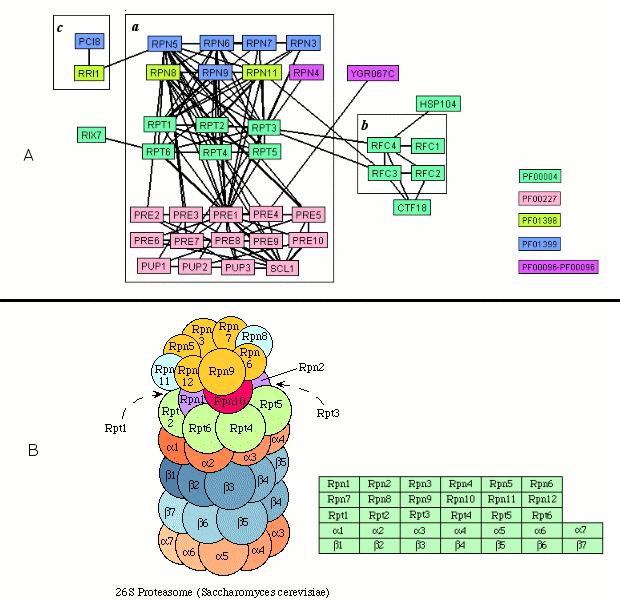
88 78

89 it implied that the 26S proteasome is a very ancient protein complex, and was well conserved in terms of both domain composition of individual proteins and composition of member proteins in the whole complex. In addition, again, different instances of a network motif can function differently. Four subunits of Replication Factor C (RFC) (CYGD ) are shown in Figure 3.10, but not Ctf18. Actually, both Ctf18 and Rfc1 can form instances of the same network motif (PF00004, PF00004, PF00004), along with other RFC proteins. Ctf18 is a subunit of a complex with Ctf8 that may be able to replace Rfc1 to form an alternative RFC along with other four subunits (Mayer et al. 2001). Interestingly, proteasome proteins Rpt1-6 formed different instances of the same network motif as well. 3.4 Discussion Using the comprehensive, well studied yeast protein interaction data, it was demonstrated that combinations of certain protein domains were frequently reused, and in many cases play different functional roles. Co-duplication of interacting partners followed by divergent evolution may contribute to many of these observations (Fryxell 1996; Caffrey et al. 1999). This work presents a novel approach to uncover duplicated pathways and protein complexes at different evolutionary distances. Redundant pathways may also be detected using this approach combined with other functional analysis. On the other hand, novel pathways may be assembled through the interaction domains (Pawson et al. 2003), and certain combinations of protein domains could be optimally suitable for some biological functions (Huang et al. 1996). Therefore, these combinations may be accumulated by natural selection, and emerge from convergent evolution (Conant et al. 2003). Further systematic studies on the evolutionary relationships among instances of 79

90 network motifs are necessary to test these hypotheses. In addition, the design of a multilevel protein similarity system easily enabled us to explore different possibilities, compared with other methods based on sequence alignment (Kelley et al. 2003; Li et al. 2005). A second major insight of this analysis was that complex systems, such as pathways and protein complexes can be built up with small modules, such as instances of small network motifs, as shown in cases like MAPK pathways and proteasome. This strategy provides us with another approach to dissect large systems into small and relatively independent units, and then again reassemble it. This type of decomposition would greatly simplify both experimental and theoretical works (Huang et al. 1996; Lahav et al. 2004). In summary, as motivated by the theory of pathway evolution, a new strategy was proposed to study the modularity of molecular networks through integration of different data types. Some insights into the organization of the biological networks started to emerge upon further analysis of predicted network motifs. Detailed analyses on more datasets from different species may shed light on the evolution of biological networks (Sharan et al. 2005). 80

91 Chapter 4. Detecting Network Motifs in Gene Co-expression Networks through the Integration of Protein Domain Information 4.1 Introduction Microarrays that characterize gene expression have provided a revolutionary approach for measuring the mrna levels of thousands of genes at the same time. Systematic analysis of genome-wide expression profiles across multiple conditions, together with integration with other kinds of data, should help provide insight into biological networks. Functionally related genes could be clustered together based on similar expression profiles. Additional information, such as the Gene Ontology (GO) can typically be exploited to help further biological interpretation of gene clusters if the target organism is well studied, such as yeast, mouse and human, but this data is often not sufficiently available for other model organisms. Moreover, general clustering algorithms produce clusters of a relatively large size, making it difficult to test these clusters using experimental methods. In addition, general clustering algorithms do not provide reasonably detailed information about the relationship among genes in a cluster, such as if some genes directly interact with each other and how. This makes it even more difficult for individual researchers to verify the associations among genes predicted by clustering algorithms experimentally. Additional independent information is needed to break big clusters into smaller ones, and thereby provide more detailed insights into relationships among genes within subclusters. Protein sequence information is a good source of additional data. Proteins can be decomposed into protein domains, which are both the units of protein function and 81

92 evolution. More importantly, there is considerable evidence that biological systems build various functional units by reusing protein domains in different combinations (Pawson et al. 2003). It is possible to decode the common mechanisms used in biological systems through studying protein domains. Duplication and divergence are important components in the evolution of genomes and biological complexity. Duplicated genes can retain or change their interaction partners. They may, over time, replace interaction partners, but the duplicated gene might still interact directly or indirectly with a partner having similar characteristics to the original partner. Multiple instances of MAP3K-MAP2K-MAPK three-tiered cascades constitute a well studied example (Chang et al. 2001). It is still unknown whether it is a general principle in biology that different genes form instances of common patterns, such as in MAPK pathways. In this study, a novel algorithm is developed to decompose the clusters of genes into smaller ones by integrating protein domain information into the clustering algorithm. This algorithm is able to provide more detailed information about putative relationships among genes within clusters by examining corresponding protein domain function. In addition, the evidence is provided that some units of similar function are temporally regulated differently at the transcriptional level. To increase confidence, this approach is able to integrate additional information, such as protein interaction data from different species. Yeast is a good source, because rich information has been already collected. 82

93 4.2 Materials and Methods Co-expression networks In a co-expression network, the genes are represented by vertices (nodes). An unweighted and undirected edge (connection) is placed between two genes if they are coexpressed, as determined by having a correlation higher than some specified threshold. A malaria transcriptome expression data set (Bozdech et al. 2003) was downloaded from the CAMDA 04 website ( and the Complete Dataset was used in this study. All Cy5/Cy3 ratio intensities were log 2 transformed. For ORFs represented by multiple oligonucleotides on the DNA microarray, the expression ratios were averaged. Pairwise correlation coefficients were calculated between all pairs of genes using the standard Pearson method. Correlation coefficients between pairs of genes computed with fewer than 33 of 46 timepoints (approximately 75%) due to missing values were discarded. The final correlation matrix had 3,842 unique ORFs after removing those genes which did not share 33 or more non-missing datapoints with at least one other gene. Based on a selected cutoff value, the calculated correlation matrix was converted into a binary symmetric matrix of the same size. An entry in this matrix was set to 1 if the corresponding correlation coefficient was greater than or equal to the cutoff value, otherwise the entry was set to 0. Rows (columns) with all-zero entries were deleted from the binary matrix, corresponding to the elimination of isolated vertices in the graph associated with such a matrix Protein domain annotation Plasmodium falciparum protein sequences and GO annotations were downloaded from PlasmoDB ( To get protein domain annotations, all protein 83

94 sequences were searched against the Pfam HMM library (Release 14.0, global, ls mode, Pfam-A HMMs with a total of 7,459 families) using hmmpfam, a program provided by HMMER package. The trusted cutoffs built in the Pfam library were employed. The HMM library was downloaded from Pfam website ( HMMER was downloaded from The computation was done on a Cluster of 32 nodes that is part of the SInRG project ( at the University of Tennessee Network motif discovery The concept of network motifs was proposed by Alon s group in studying various real world networks, including biological networks (Milo et al. 2002; Shen-Orr et al. 2002). Network motifs were defined as patterns of interactions recurring more frequently in a network than in randomized networks. Here, the concept of a network motif was extended to labeled graphs by studying patterns of vertex labels (Figure 4.1). As shown in Figure 4.1A, a hypothetical network motif might be a clique of three genes. These genes are highly co-expressed, as required by the correlation cutoff to create an edge. In addition, each gene has its own characteristic protein domain information as reflected in its label. Figure 4.1B shows 7 hypothetical genes in a co-expression network forming three distinct instances of the network motif, as described in Figure 4.1A. In each of the instances, three genes are highly correlated with each other as indicated by the edges, and their protein domain information maps one-to-one to the specified network motif based on rules, as described below. Among the three instances, instances II and III share at least one gene (here two genes), and these two instances are defined as overlapping. On the 84

95 Figure 4.1 Schematic of a network motif in gene co-expression networks. (A) A network motif is a pattern as a complete connected subgraph (e.g. cliques) of certain size k (k = 3 here) and the vertices are labeled as reflected by the shapes and shadings. Here vertices represent genes and the vertex labels are the protein domain information of the proteins encoded by the corresponding genes. (B) Seven hypothetical genes in a co-expression network forming three distinct instances of the network motif as described in (A). In each of the instances, three genes are highly correlated with each other as indicated by the edges, and their protein domain information maps one-to-one to the network motif. Instances II and III share at least one gene (here two genes) and these two instances are defined as overlapping. Instance I does not share any genes with instance II, so these two are non-overlapping. Instances I and III form another pair of non-overlapping instances. 85

96 86

97 other hand, instance I does not share any genes with instance II, so these two are nonoverlapping. Instances I and III form another pair of non-overlapping instances. In general, it is insisted that in a network motif of size k (k = 3 in the above example) every pair of vertices is joined by an edge, that is, the network motif forms a clique. Starting from the above calculated P. falciparum co-expression network, it was first converted into a labeled graph whose vertices (genes) were labeled with their corresponding annotated Pfam protein domain information. The clique-based clustering algorithm of (Langston et al. 2005) was applied to this labeled co-expression network, to search for patterns of highly co-expressed genes or network motifs (Figure 4.1). For a specified k, all k-vertex cliques were scanned and grouped based on the protein domain information. Within a group of cliques, protein domain information in each clique can match one-to-one against protein domain information of genes in any other clique. These groups of cliques are called putative network motifs. Next, a parameter f specifying the minimum number of mutual non-overlapping instances in a network motif was used to trim the list of putative network motifs. Only putative network motifs having at least f non-overlapping instances were kept as network motifs. To account for the abundances of different domains in the whole genome, the statistical significance of each detected network motif was further assessed by comparison to randomized networks. Starting from the real co-expression network, a randomized network was generated by randomly permuting the domain labels of all genes while leaving the connection structure of the graph untouched, and then the same network motif detection procedure was run on the resulting randomized network. This 87

98 process was repeated 1,000 times. The fraction of times the same network motif was found in the randomized networks was defined as the p-value for the network motif. Matching of protein domain information between two genes can be classified into many possible levels, but what was proposed here are only domain matching levels A and B. Level A requires that two proteins have the exact same type of domain, the same number of each type of domain, and all domains in the same order in the respective protein sequences from N-terminal to C-terminal. Domain matching level A is a global alignment that suggests that the two proteins are essentially the same in terms of domain architecture. Domain matching level B only requires the same types of domain, with no constraints on the number and the order of domains in the proteins. At this level, the domain duplication and domain shuffling during evolution are permitted while suggesting that the basic molecular functions of each protein might be similar. The network motif detection procedure was run separately using different domain matching levels Protein interaction networks A yeast protein interaction dataset was downloaded from the BIND website ( In this protein interaction network, genes were again represented by vertices (nodes). An un-weighted and undirected edge (connection) was placed between two genes if there was a documented interaction between these two genes. Since the topologies of most protein complexes are unknown at this time, protein complexes were converted into binary interactions using the matrix model, which put edges between all possible pairs of genes in the same protein complex (Bader et al. 2002). The use of the matrix model facilitates searching for possible instances of network motifs 88

99 found in co-expression networks in protein complexes. Yeast GO annotations were downloaded from SGD ( Data visualization Detected network motifs are presented on the web using ALIVE ( Expression plots were drawn using R ( 4.3 Results Co-expression networks To convert a correlation matrix into a corresponding binary co-expression network, a suitable cutoff value for the correlation coefficient must be chosen. Based on the previous reports that biological networks, including co-expression networks, follow a scale-free distribution of connectivity (Bhan et al. 2002; Lee et al. 2004), a cutoff value was chosen that gave fewer vertices with a higher degree (connectivity). Plots of the degree distribution for graphs generated under a series of cutoff values suggest that a correlation cutoff value of 0.95 is appropriate through visual inspection (Figure 4.2). This value was surprisingly higher than what was expected. When comparing the distribution of correlation coefficients of this dataset with those of several cell/life cycle gene expression datasets, it was found that the distribution of correlations in this dataset showed a characteristic bimodal shape while others had a bell-like shape (Figure 4.3). One of the possible reasons is that the majority of genes in this dataset exhibit periodicity (Bozdech et al. 2003). Within this data set and others, it was observed that genes which exhibit periodicity tend to shift the distribution toward higher correlations. When the genes in the Overview Dataset that were selected based on their strong periodic behavior 89

100 Figure 4.2 Degree distributions of co-expression networks generated under different cutoff values of correlation coefficients (R). For each cutoff value (shown at the bottom of each plot), a co-expression network was generated (see the main text for details), and the histogram of the degrees of all vertices (the numbers of connections of vertices) was plotted using R with default settings. The horizontal axis is the vertex degrees and the vertical axis is the relative frequencies. 90

101 Figure 4.3 Survey of distributions of Pearson's correlation coefficients for several timeseries gene expression datasets. Both "complete and overview were malaria P. falciparum life cycle microarray dataset from (Bozdech et al. 2003). complete was the complete dataset and overview was the overview dataset reported in the study. Both rochall and rochdf were malaria P. falciparum life cycle microarray data from (Le Roch et al. 2003). rochall contained all genes probed on the array while rochdf contained only differentially expressed genes in the study. Both hsall and hscc were human cancer cell line (Hela) cell division cycle microarray data from (Whitfield et al. 2002). hsall was the complete dataset and hscc was the dataset with only cell cycle regulated clones. yeast was the combined yeast cell cycle microarray data from (Spellman et al. 1998) and (Cho et al. 1998). 91

102 92

103 were removed, the degree distributions of those resulting networks did tend to have fewer vertices of higher degrees compared to the original networks (Figure 4.4). It was further verified that the resulting co-expression network (R 0.95) was enriched (p-value < 0.001, chi-square test) with genes of periodic behavior. About 93% (2,124 of 2,292) of unique ORFs in the co-expression network (R 0.95) are in the Overview Dataset of 2,714 ORFs (about 78%) while only about 36% (559 out of 1550) of those genes removed by this cutoff were in the Overview Dataset Prediction of network motifs Using a series of values for parameters k, the size of network motifs and f, the minimum number of non-overlapping instances, a number of putative network motifs were found under different domain matching levels (Table 4.1). As shown in Table 4.1, both increasing k and f decrease the number of network motifs detected (first number in each cell). More network motifs were found at domain matching level B than at level A with the same corresponding parameter values for k and f, probably because of the less stringent constraints on matching protein domain information. More studies are needed to check if a better coverage is achieved at domain matching level B by including more distantly related genes, or it just simply adds more noise. The majority (>95%) of putative network motifs have p-values less than 0.05 in all cases. It was assumed that genes in the same instance of a network motif should share the same biological process if they are indeed functionally related, though each gene may have different molecular functions. Therefore, the biological relevance of the putative network motifs was evaluated by simply counting the number of genes within an instance that share the same GO terms in a biological process category. Although the GO 93

104 Figure 4.4 Degree distribution of co-expression networks generated under different cutoff values of correlation coefficients (R) when those genes in the Overview Dataset were removed because of their strong periodic behavior. For each cutoff value (shown at the bottom of each plot), a co-expression network was generated (see the main text for details), and the histogram of the degrees of all vertices (the numbers of connections of vertices) was plotted using R with default settings. The horizontal axis is the vertex degrees and the vertical axis is the relative frequencies. On the top of each plot are the number of edges (E) and vertices (V) in the corresponding network. 94

105 Table 4.1 Summary of the number of putative network motifs detected with different set of parameter values. Domain matching level A k = 3 k = 4 k = 5 k = 6 f = 2 88, 25 18, 11 6, 5 1, 1 f = 3 3, 2 0, 0 0, 0 0, 0 Domain matching level B k = 3 K = 4 k = 5 k = 6 f = 2 197, 53 87, 29 32, 17 9, 6 f = 3 17, 13 6, 6 0, 0 0, 0 f = 4 5, 5 0, 0 0, 0 0, 0 k: the size of network motifs to search for. f: the minimum number of mutual nonoverlapping instances for a network motif. Within each cell the first number is the number of network motifs found in malaria co-expression network (R 0.95) with the corresponding parameter values, and the second number is the number of those network motifs having at least one instance in the yeast protein interaction network. 95

106 annotations on malaria genes are relatively limited, it can still be observed that genes with GO annotations in the same motif instance did tend to share similar terms. Also the functional gene groups as provided in (Bozdech et al. 2003) was used to check the similarity of functions of genes in the same instances, and this gave similar results. Figure 4.5A shows a putative network motif detected under domain matching level A, k = 6 and f = 2. This motif consists of six highly co-expressed genes. Three of six genes have the same domain combination as two domains ordered from N- to C-terminal, DEAD/DEAH box helicase (PF00270) and Helicase conserved C-terminal domain (PF00271). These genes are involved in various aspects of RNA metabolism as suggested by the Pfam domain annotation. One of the six genes has three WD domains, G-beta repeats (PF00400), one has a Brix domain (PF04427) and the last one has a GTPase of unknown function (PF01926). The protein domain functions suggest that this network motif is involved in ribosome biogenesis (Neer et al. 1994; Eisenhaber et al. 2001). Figure 4.5B shows the P. falciparum genes form various instances of the network motif through different combinations of genes. (Genes are shaded in the same way as the Pfam accession numbers shown in Figure 4.5A to indicate their corresponding domain information). Only 5 of 13 genes were assigned with functional group annotation and all of these five genes were in the Cytoplasmic Translation Machinery functional group (Bozdech et al. 2003). Only 3 of the 13 genes have GO annotations. Significantly, these three genes are a subset of the group of five, and were all assigned with the same GO terms: RNA metabolism (GO:16070), nucleobase, nucleoside, nucleotide and nucleic acid metabolism (GO:6139), cell growth and/or maintenance (GO:8151) and metabolism (GO:8152). These GO annotations are very broad, but agree with the more specific 96

107 Figure 4.5 An example network motif. (A) A putative network motif detected at domain matching level A with parameter values k = 6 (size) and f = 2 (minimum number of mutual non-overlapping instances). This network motif consists of six highly coexpressed genes and three of them have the same domain combination as two domains ordered from N-terminal to C-terminal, DEAD/DEAH box helicase (PF00270) and Helicase conserved C-terminal domain (PF00271). One of the six genes has three WD domains, G-beta repeats (PF00400), one has a Brix domain (PF04427) and the last one has GTPase of unknown function (PF01926). (B) Thirteen P. falciparum genes form various instances of the network motif through different combinations of genes. Genes are shaded in the same way as those Pfam accession numbers shown in (A) to indicate their corresponding domain information. (C) The expression profiles of those 13 genes. 97

108 98

109 hypothesis that these genes are related to ribosome biogenesis. This group of 13 genes may potentially work together in some way, since they all had very similar expression profiles under these diverse developmental stages. It is also possible that these genes were organized as several small functional units. More information is needed to dissect this cluster of genes, but this analysis might suggest some initial inferences with which to guide future experiments Confirmation of prediction by yeast protein interactions It was hypothesized that a predicted network motif would be more likely to be true if it appears in other independent datasets. It will provide further support to those predicted network motifs if they appear in a dataset from other species, since protein-protein associations may be transferred across organisms (von Mering et al. 2005). One of the advantages of treating protein domains as functional units of proteins, and labeling genes with their protein domain information is the flexibility of doing cross-species comparisons across significant evolutionary distances. To gain further confidence in these predictions, the yeast protein interaction data was chosen to be searched for instances of putative malaria network motifs, since it included rich protein complex information. The second number in each cell of Table 4.1 shows the number of malaria network motifs having instances in the yeast protein interaction network. It can be seen that relatively more malaria network motifs were supported by the yeast interaction data as the parameters became more stringent. The matrix model increased the coverage of the yeast proteome by including all possible true interactions within the experimental data, but some false interactions were also added (Bader et al. 2002). This model was considered to be the best compromise for module discovery. The results from the protein 99

110 interaction data should be further studied individually, especially when there is better experimental verification. Figure 4.6 shows the instances formed by different combinations of 27 genes detected in the yeast protein interaction network for the malaria network motif shown in Figure 4.5. Forty-five protein complexes stored in the BIND database have at least two members belonging to this group of 27 genes. This strongly suggests that these gene products directly interact with each other under different conditions in various ways. One extreme example is that protein complex contains six genes forming an exact instance of the predicted network motif. The two largest groups of genes sharing a common GO annotation in this group of 27 genes are a group of 9 genes annotated as ribosomal large subunit assembly and maintenance (GO:27) and the other 8 genes as 35S primary transcript processing (GO:6365). These two groups totally cover 13 out of 27 genes. All of the evidence above suggests that this particular network motif represents a core interaction unit for various protein complexes involving cytoplasmic translation, or even more specifically as ribosome biogenesis. This supports tentative functional assignment of all the involved malaria genes that had no prior annotation. The strength of this strategy is both to cluster functionally related genes, and to provide more detailed information about relationships among these genes by integrating information from multiple orthogonal sources Prediction of complementary functional units A network motif represents a specific combination of individual protein domains, and this combination can carry out a special function shared by individual instances as relatively independent subsystems. It was hypothesized that individual instances of a 100

111 Figure 4.6 Instances found in the yeast protein interaction network for the network motif shown in Figure 4.5. (A) The similar yeast network motif as shown in Figure 4.5. (B) A subgraph of the yeast protein interaction network was shown, and only included vertices (genes) forming at least one instance of the network motif. Yeast genes are shaded in the same way as in Figure 4.5A to indicate their corresponding domain information. Highlighted is an instance of the network motif in which all six proteins present in the protein complex in BIND database. 101

112 network motif could function in different locations and times, depending upon their regulation. The malaria time series data enabled the testing of this hypothesis by examining the temporal expression profiles of instances of network motifs. Figure 4.7 shows such an example network motif detected at domain matching level B with parameter values k = 3 and f = 2. This network motif represents a combination of three independent domains, AhpC/TSA family (PF00578), protein kinase domain (PF00069) and Calcineurin-like phosphoesterase (PF00149) (Figure 4.7A). Six P. falciparum genes form two independent instances of this network motif (Figure 4.7B). The AhpC/TSA family contains Peroxiredoxins (Prxs), a ubiquitous family of antioxidant enzymes which can be regulated by phosphorylation (Wood et al. 2003). The paired kinase and phosphatase may reflect that these two Prxs are tightly controlled through phosphorylation and dephosphorylation. Of striking interest is that apparently these six genes all have similar expression profiles, and the only major difference is the timing. There is a phase difference between two instances, while all three genes within each of the two instances have very similar timing. When these expression profiles are compared with morphological data (Bozdech et al. 2003), one could conclude that one instance (PF08_0131, PFD0865c, PFA0390w) functions at the trophozoite stage, and another (PF14_0142, PFC0775c, PFL0725w) at the schizont stage based on their peak expression values. Having instances in the yeast protein interaction data provides further support that these genes do interact directly (Figure 4.7D). It is worth mentioning that none of these genes were assigned to a functional group (Bozdech et al. 2003), and these six genes share very broad GO annotations such as cell growth and/or maintenance (GO:8151) and metabolism (GO:8152). 102

113 Figure 4.7 Instances of a network motif showing different expression profiles. (A) A network motif detected at domain matching level B with parameter values k = 3 and f = 2. This network motif represents a combination of three independent domains, AhpC/TSA family (PF00578), protein kinase domain (PF00069) and Calcineurin-like phosphoesterase (PF00149). (B) Six P. falciparum genes form two instances of this network motif. (C) Expression profiles of these six genes. (D) Instances of the network motif were found in yeast protein interaction network. 103

114 4.4 Discussion With the rapid development of high-throughput methods, such as microarrays, massive amounts of experimental data have been collected for different species under various conditions. New computational approaches are needed to analyze this data in an integrative way, and provide more reliable results with finer resolution for experimental verification. Here, a new strategy is proposed to analyze gene expression data by integrating a diversity of additional information, such as primary sequence information and protein interaction data. Though the present study starts with a dataset from a single species, this approach is used here to look for patterns in other species, and can be easily generalized to begin with information from multiple species. The strategy of integrating protein domain information into expression data analysis was based on the hypothesis that genes/proteins form relatively independent functional modules. Gene expressions within these modules will be well coordinated because of selective forces or functional constraints. The possible origins of these modules are gene duplication and the reuse of protein domains. This then implies that these modules might form some common patterns at the protein domain level that can be observed in experimental data. Those relatively detailed predictions of association among genes as shown in Figure 4.7 provide rich information for experimental verification and elucidation by examining other data in light of these presumptive network motifs, including studies of networks under other conditions. Several things can be done to refine this analysis. For example, it might be possible to combine instances of these motifs together toward building up larger network components, such as large pathways or protein complexes. It should be allowed to loosen the strict requirements for exact cliques 104

115 for motifs of interest, as evolution will not always preserve exact co-expression matches, and not all members of a motif will be duplicated. It is believed that the general approach that has been outlined here can become a useful tool to ask a number of other interesting research questions about how networks work in the present time, and how they arose to work that way over evolutionary time. 105

116 Chapter 5. Differential Expression of Parallel Functional Modules in Mouse Tissues 5.1 Introduction One of the major factors that contribute to genome complexity is gene duplication (Ohno 1970). Duplicated genes may encode proteins with redundant functions, even though they may have diverged in their gene expression after the duplication event (Gu et al. 2002). When a set of proteins that function together in a pathway or complex are duplicated and modified, parallel modules of similar function may arise. The aim here is to explore the extent of differential gene expression of such parallel modules. Previously, paralogous pathways were identified from budding yeast protein-protein interaction networks constructed from experimental data (Kelley et al. 2003). A network comparison method was used to align the yeast network to itself. Three hundred highscoring paralogous pathways were detected when requiring pairs of proteins have BLAST E-values no greater than and that there is a conservation of interactions between paralogous pathways. A more recent work identified parallel modules from protein functional linkages, which were computationally inferred from genome sequences (Li et al. 2005). Proteins in parallel modules were paired up based upon their phylogenetic distances. Here, a novel strategy is applied to predict parallel functional modules. Instead of using sequence alignment as described above, a linear protein sequence is decomposed into a collection of protein sequence domains. These domains are both the functional units and evolutionary units of protein sequences (Chothia et al. 2003). The concept of 106

117 network motif (Milo et al. 2002; Shen-Orr et al. 2002) is extended to detect network modules in the integrated molecular networks. Instead of using unlabeled graphs (Milo et al. 2002; Shen-Orr et al. 2002), proteins and genes are first labeled with their corresponding protein domain information (Figure 5.1). The next step is to search for frequently occurring patterns of interacting protein domains, or network motifs. Each network motif has multiple instances, and each instance is a connected subgraph in the network being studied. For each instance, the protein domain information of member proteins can one-to-one map to the network motif. Instances of the same network motif are defined as parallel modules. These parallel modules may be able to carry out similar functions, but under different conditions. For example, multiple instances of the three-kinase module in mitogen-activated protein kinase (MPAK) pathways can be composed of different sets of proteins, and each set of protein kinases functions under one set of conditions (Widmann et al. 1999). The availability of the comprehensive transcriptomes across a wide range of tissues (Su et al. 2004) provides an opportunity to study the differential expression of multiple instances of the same network motif. If these instances are expressed in different tissues, it provides evidence that they may carry out similar functions at different locations. Using an integrated approach, network motifs are first identified in a mouse proteinprotein association network (von Mering et al. 2005). It is then demonstrated that different instances of the same network motif were differentially expressed in multiple mouse tissues (Su et al. 2004), even when these instances were annotated to the same pathway. Also, previous work is advanced to search for tissue-specific network motifs in the gene co-expression network constructed from the mouse tissue transcriptome (Su et al. 107

118 Figure 5.1 Definition of a network motif. (A) A network motif represents a combination of domain information. (B) Instances of the network motif in a protein-protein association network (PPA). In a PPA network, the proteins are vertices (nodes). Two proteins are connected by an edge (connection) if they are functionally associated to each as documented in the database. Here, the PPA network is a labeled network with nodes (proteins) being labeled with their corresponding domain information. Each instance of a network motif is a connected subgraph within the labeled PPA network, and the protein domain information of proteins in the subgraph can one-to-one map to the network motif. (C) Instances of the network motif in a gene co-expression network. In a gene coexpression network (GCE), the genes are vertices (nodes). An un-weighted, and undirected edge is put between two genes if they are co-expressed with a correlation coefficient greater than a specified threshold. The GCE network is labeled the same way as a PPA network in (B). Each instance is defined the same way as that in (B), but adding the restriction that the connected subgraph has to be a complete subgraph (a clique). This ensures that all genes of an instance are highly co-expressed as required by the correlation cutoff to create an edge. Among the three instances, instances II and III share at least one gene (gene 5 here), and these two instances are overlapping with each other. On the other hand, instance I does not share any genes with instance II, so these two are non-overlapping. For a network motif, the size k is defined as the number of proteins or genes in any one of its instances. Another parameter associated with a network motif is f, which is defined as the minimum number of mutual non-overlapping instances. 108

119 A. Network Motif {,, } Protein domain α Protein domain β and γ Protein domain θ B. Instances in Protein-Protein Association Network Protein 1 Protein 4 Protein 7 Protein 2 Protein 3 Protein 5 Protein 6 Protein 6 Protein 8 I II III C. Instances in Gene Co-expression Network Gene 1 Gene 4 Gene 7 Gene 2 Gene 3 Gene 5 Gene 6 Gene 5 Gene 8 I II III 109

120 2004). This study provides evidence that parallel modules are spatially regulated differently at the transcriptional level. This study also sheds some light on how to identify alternative pathways or complexes. 5.2 Materials and Methods Protein-protein association network Mouse protein-protein association data were downloaded from the STRING database (release 5.1, high confidence or better) (von Mering et al. 2005). The STRING database is a comprehensive collection of known and predicted protein-protein associations. Selfself interactions were removed and SwissProt/EnsEMBL identifiers of proteins were converted into LocusLink (NCBI, NIH, Bethesda) identifiers using the GeneKeyDB (GKDB) database (Kirov et al. 2005). In total, 3,568 loci and 7,452 interactions remained in the network. In the protein-protein association network, the proteins are vertices (nodes). Two proteins are connected by an edge if they are functionally associated with each other, as documented in STRING Mouse tissue expression dataset The mouse tissue gene expression data were obtained from a recently published series of Affymetrix microarray experiments done by the Genomics Institute of the Novartis Research Foundation (Su et al. 2004). In total, 61 mouse tissues were profiled. The levels of expression were recorded as average difference (AD) values. Affymetrix probe identifiers were mapped to individual loci in the mouse genome using the LocusLink database (NCBI, NIH, Bethesda). Probes with ambiguous mappings were removed. A total of 14,725 mouse loci were one-to-one mapped to their probe identifiers. A gene was 110

121 defined as expressed in a tissue if its average AD value was at least 200 (Su et al. 2002). In total, 12,873 genes were expressed in at least one of the 61 tissues Mouse gene co-expression network In a co-expression network, the genes are vertices (nodes). An unweighted, undirected edge (connection) is put between two genes if they are co-expressed with a correlation coefficient greater than a specified threshold. Before creating the mouse gene co-expression network, the mouse tissue gene expression data, as described above, was further processed as follows. To take advantage of repeated measurements, an analysis of variance was done to select those genes with AD values significantly varied among tissues (p < 0.001), using R ( This was to ensure the variation in expression values was mainly from tissues. Repeated measurements of the same tissue samples were then averaged. Unexpressed genes (AD values < 200 in all tissues) were removed. The averaged AD values of the remaining genes were clipped at a value of 20 (Su et al. 2004). To ensure genes were differentially expressed among tissues, nondifferentially expressed genes (maximum AD/minimum AD < 10) were further filtered out (Jordan et al. 2004). A total of 8,053 mouse loci were left. For each gene, AD values were normalized by taking the log2 value of the ratio of tissue-specific AD value/median AD value for all tissues. The correlation between gene expression profiles was calculated using the standard Pearson method Protein domain annotation Mouse protein sequences were downloaded from the RefSeq database (NCBI, NIH, Bethesda). GO annotations were downloaded from the LocusLink database (NCBI, NIH, Bethesda). To obtain protein domain annotations, all protein sequences were searched 111

122 against the Pfam HMM library (Release 14.0, global, ls mode, Pfam-A HMMs with a total of 7,459 families) using hmmpfam, with trusted cutoffs according to Pfam. The HMM library was downloaded from the Pfam website ( HMMER was downloaded from The computation was done on the OIT Cluster of 32 nodes of the SInRG project ( Network motif discovery The prediction of network motifs in the protein-protein association network was done in the same way as in Chapter 3. The prediction of network motifs in the gene coexpression network was done in the same way as in Chapter 4. To detect network motifs with instances of tissue-specific expression, it was further required that there was no edge between at least two sets of instances of the same network motif. In addition, at least one pair of genes was required to have a correlation coefficient less than zero, where these two genes were from any pair of instances of the network motif. For all predictions, the same parameter values were used, with k = 3 (the size of a network motif) and f =2 (the minimum number of mutual non-overlapping instances in a network motif) Graph randomization To account for the abundance of different domains in the whole genome and the density of connections of different genes in those networks, the statistical significance of each detected network motif was further assessed by comparing it to randomized networks generated with four different algorithms, as described in Chapter

123 5.2.7 Protein-Protein similarity The matching of protein domain information between two genes can be classified by many possible methods, but here two proteins were defined as a match if they have the same types of domains. No constraint was placed on the number and the order of domains along the protein sequences. Domain duplication and domain shuffling events that occurred during evolution were thus considered, while ensuring that the basic functions of two proteins were comparable Gene Ontology similarity Gene Ontology (GO) similarity scores of a set of genes/proteins were calculated in the same way as in Chapter 3. Two datasets were generated as controls. The first control had 10,000 sets of three distinct, randomly chosen genes or proteins with replacement, and the second one contained 10,000 connected subgraphs randomly chosen with replacement from the same network being analyzed. For each control, GO similarity scores were calculated for all those sets of three genes. The non-parametric two-sample Wilcoxon test was used to estimate if the GO similarity scores of one sample tend to be larger than those of another, using R (Ihaka et al. 1996) Data visualization Detected network motifs were visualized using ALIVE ( Expression plots were drawn using R. 113

124 5.3 Results Differential expression of network motifs from protein-protein association networks We obtained 260 putative network motifs after carrying out a comprehensive search for small network motifs (k = 3, f = 2, see methods) in the mouse protein-protein association network, which was constructed using the STRING database (von Mering et al. 2005). The cutoff p-value was arbitrarily chosen as 0.01, since it produced a reasonable number of network motifs (243), for the following statistical analysis. It was assumed that each set of functionally related proteins should be annotated with similar Gene Ontology (GO) terms in the biological process category. Considering that proteins with the same domain annotations may have similar GO annotations, the GO analysis was restricted to the subset of predicted network motifs made of all three different labels of domain information. It was verified that the proteins within each instance of significant network motifs (p < 0.01) tended to be annotated to similar biological processes, even though they all had different protein domains, when compared to randomly chosen connected subgraphs in the same network. (one-sided Wilcoxon test, p < 0.001) (Figure 5.2). It was hypothesized that different instances of the same network motif may have similar functions, but exist at different locations, such as in different tissues. It was assumed that all of the genes within an instance had to be expressed in the tissue in which the instance functions. Figure 5.3 shows a network motif related to the TGF-beta signaling pathway. It demonstrates a canonical form of interactions in TGF-beta pathways: ligands of TGF-beta family (PF00019-PF00688) interact with receptor kinases 114

125 Figure 5.2 Histogram of GO similarity scores of instances in three datasets: 1) instances of those predicted network motifs with 3 different domain labels (mt, green diamond), 2) 10,000 sets of three randomly chosen proteins from the yeast PPI network (rnd, black circle) and, 3) 10,000 randomly chosen connected subgraphs (cc, red square) from the mouse protein-protein association network in the biological process category. Bin labels on the horizontal axis are the upper bound for each bin (e.g., the label 0.8 indicates 0.7 < Score 0.8). 115

126 Figure 5.3 An example network motif related to the TGF-beta signaling pathway. Top: overview of the network motif. Information about protein domains: PF00019: Transforming growth factor beta like domain. PF00688: TGF-beta propeptide. PF00069: Protein kinase domain. PF01064: Activin types I and II receptor domain. PF03165: MH1 (MAD homology 1) domain. PF03165: MH2 (MAD homology 2) domain. Bottom: the expression profiles of different instances (rows) of the network motif as shown on the top across different tissues (columns). At the right end of each row are the names of member proteins in each instance. 116

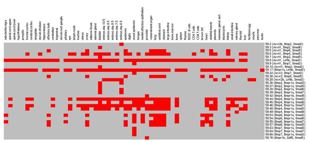
127 117

128 (PF00069-PF0064), and downstream proteins of the SMAD family (PF03165-PF03166) mediate TGF-beta signaling (Massague 1998). Combinations of proteins from each of these three protein families formed different instances of the network motif, and instances were expressed in different tissues. This implied that some proteins had alternative partners in different tissues. Some tissues, such as liver, had multiple instances of the same network motifs (Figure 5.3). These predictions were also systematically searched against known pathways. An instance was defined as being mapped into a known pathway if all of the proteins in the instance were found within the same pathway, based on information from either KEGG (Kanehisa et al. 2000) or BioCarta ( Seventy out of 260 putative network motifs had at least one instance, which was mapped into a known KEGG or BioCarta pathway, and all 70 network motifs were statistically significant (p < 0.01). To ensure that different instances have similar functions, the analysis was restricted to survey those pairs of instances that were from the same network motif and mapped into the same known pathway. Also, each of these instances was expressed in at least one of the 61 tissues in the data set. Mapping into known pathways, and co-existence of mrnas may be considered as a method to filter out false positive predictions. For every possible pair of instances as described above, the number of differentially expressed tissues was calculated, i.e. the number of tissues in which it had only one instance of the pair expressed. Figure 5.4 shows the number of differentially expressed tissues for all 43,156 qualified pairs of instances from 51 predicted network motifs. Those instances were mapped into 39 known pathways. The number of differentially expressed tissues was less than that of randomly chosen pairs of instances (p < one-sided Wilcoxon test). 118

129 Figure 5.4 Histograms of the number of tissues in which the pairs of instances were differentially expressed. On the left: motif refers to the dataset of all 43,156 pairs of instances in which each pair satisfied the following three conditions 1) both instances of the pair were from the same network motif, 2) each of the two instances were expressed in at least one tissue, 3) both instances were mapped into the same known pathways (KEGG or BioCarta). control refers to the dataset of 9,991 randomly chosen pairs of instances in which each instance was expressed in at least one tissue. Mean ± SD: 11.6 ± 12.8 (motif), 20.4 ± 15.3 (control). On the right: the same as the left plot, but the pairs of instances were excluded if two instances shared one or more proteins. In total 17,160 pairs from motif dataset were kept, and 8,950 pairs for control dataset. Mean ± SD: 11.6 ± 12.7 (motif), 21.3 ± 15.5 (control). Bin labels on the horizontal axis are the lower bound for each bin (e.g., the label 0 indicates 0 Score < 5). 119

130 5.3.2 Prediction of network motifs with tissue-specific instances Considering the incomplete coverage of protein interactions in the mouse genome by the STRING database, prediction of network motifs based on the mouse tissue gene expression data itself (Su et al. 2004) was attempted. Cases where instances of the same network motifs were differentially expressed in certain tissues were searched for. To achieve this goal, network motifs were searched in the gene co-expression network constructed from the mouse gene atlas data (Su et al. 2004). To convert a correlation matrix to a corresponding co-expression network, a suitable cutoff value for the correlation coefficient had to be chosen. Based on the previous reports that biological networks, including gene co-expression networks, follow a scale-free distribution of connectivity (Bhan et al. 2002; Lee et al. 2004), a series of cutoff values were chosen for the Pearson correlation coefficient. The node degree distributions of the resulting series of networks were investigated. Plots of the degree distribution for networks generated under the series of cutoff values showed the correlation cutoff values ranging from 0.9 to 0.75 all gave a good fit to a power law distribution (Figure 5.5). As the cutoff value increased, both the total number of genes and the number of connections among genes decreased. A cutoff value of 0.75 was chosen for the following analysis, since it generated a co-expression network of high confidence, while still retaining enough genes for the subsequent analysis. In total, 4,152 genes and 86,564 edges were left in the final gene co-expression network. We carried out a comprehensive search in the mouse co-expression network using the same values for parameters (k = 3 and f = 2) used in analyzing the mouse protein-protein association network, and obtained 896 putative network motifs. Four hundred and thirty 120

131 Figure 5.5 Node degree distributions are shown for co-expression networks generated under different cutoff values of correlation coefficient (R). For each plot, on the top is the average degree of each gene in each network. In the parenthesis are the total number of degrees, and the total number of genes left in the network after applying the specified cutoff value, which is indicated at the bottom of each plot. 121

132 nine out of 896 network motifs were statistically significant (p < 0.01). GO similarity analysis was also carried out on these significant network motifs. The proteins within each instance of the predicted network motifs tended to be annotated with a similar biological process when compared to connected subgraphs in the same network (onesided Wilcoxon test, p < 0.001). This was not true when the subset of predicted network motifs comprised of all three different labels of domain information were compared to the control. This implies that the quality of predictions based only upon co-expression could still be improved in the future. A predicted network motif is shown in Figure 5.6 involving three genes encoding intermediate filament proteins (IF, PF00038). IF proteins of the same group are well known to interact with each other, and their polymerization provides a flexible intracellular scaffold to structure cells (Fuchs et al. 1998). In this example, all of the known genes are keratin genes, which in general, can be partitioned into two major types (I and II). The keratin polymers are built from those heterodimers (Coulombe et al. 2002). Consistent with the hetero-polymerization principle, all of the known type II keratin genes were highly correlated with type I keratin genes, but not other type II keratin genes, as indicated by an absence of edges between type II keratin genes (Figure 5.6). Since most type I and II keratin genes form heterodimers, the pairing of two type I genes with one type II keratin gene, as suggested by this network motif, may be an artifact of the parameter setting, since it was set to search for network motifs with 3 nodes. On the other hand, this may reflect the prevalence of a functional redundancy among keratin genes (Coulombe et al. 2002; Wong et al. 2005). For example, Krt-18 may be able to compensate for Krt1-19 as demonstrated by Krt1-19 knockout mice appearing normal, 122

133 Figure 5.6 Keratin related network motif (PF00038, PF00038, PF00038; PF00038: Intermediate filament protein). On the top is the heatmap plot representing the expression profiles across 61 tissues of genes involved in forming different instances of the network motif. Rows are genes. Columns are tissues. For each gene, red indicates that its expression was higher than the medium value and green indicates that its expression was lower than the medium value, black for equal to medium. Tissue types were labeled vertically on the top of the plot. Genes were labeled on the right of the plot in the order of: the type of keratin (? for unannotated by NCBI), LocusLink ID, Gene name and Chromosome number. At the bottom is the corresponding network motif (A) and instances (B). Refseq gene names (A) or Pfam accession numbers (B) are used as the labels for each node. Type II keratins are shaded with patterns: think lines for known type II keratin genes and fine lines for predicted ones. The rest were all type I keratins and are without shading, either known or predicted. Dashed lines represented the separation of the clusters of instances based on the expression profiles. Instances were clustered into two groups: simple epithelia-related (left) and complex epithelia-related (middle and right). The complex epithelia-related instances were further divided into two subgroups (middle and right) based the expression differences in umbilical cord and eye. 123

134 124