UNIVERISTY OF MIAMI CLIMATE FEEDBACKS IN THE SURFACE RADIATION BUDGET. Angeline Pendergrass A THESIS

Transcription

1 UNIVERISTY OF MIAMI CLIMATE FEEDBACKS IN THE SURFACE RADIATION BUDGET By Angeline Pendergrass A THESIS Submitted to the Faculty of the University of Miami in partial fulfillment of the requirements for summa cum laude Coral Gables, Florida May 2006

2 ABSTRACT PENDERGRASS, ANGELINE (B.S., Meteorology/Math, Physics) Climate Feedbacks in the Surface Radiation Budget. (May 2006) Abstract of a bachelor s thesis at the University of Miami. Thesis supervised by Professor Brian Soden. No. of pages in text: 20 The Earth s surface is an important interface for the exchange of energy and particles between the atmosphere, ocean, and land. Changes in the energy budget at the surface impact not only how the surface temperature changes, but also how cirulation changes as the planet warms. Climate feedbacks are an integral part of the surface energy balance. Water vapor, temperature, surface albedo, and cloud feedbacks are calculated using global circulation model experiments that simulate the climate in the twenty-first century when the equivalent level of carbon dioxide in the atmosphere doubles. Findings include that the largest positive feedback at the surface is from water vapor. The largest contributions to the water vapor and temperature feedbacks arise from the lowest levels of the atmosphere. Cloud feedback is the largest source of intermodel variability. General characteristics of surface feedbacks share many similarities to their counterparts at the top of the atmosphere. The main difference from the top of the atmosphere is that the feedbacks are dominated by the response near the surface, whereas at the top of the atmosphere they are dominated by the upper troposphere.

3 iii CLIMATE FEEDBACKS IN THE SURFACE RADIATION BUDGET TABLE OF CONTENTS 1. Introduction 1 a. The Surface Radiation Budget From 1824 to b. What is a GCM? 5 c. IPCC 7 d. Scenarios 7 2. Data 8 a. Models and Variables 8 b. Environmental Changes 9 c. Radiative Adjoints Methodology 13 a. Calculations Results 17 a. Global Average 17 b. Vertical structure 18 c. Cloud feedback Discussion Conclusions 20 Tables 21 Figures 24 Appendix: Individual models 43 References 49

4 1. Introduction Global warming is the idea that the temperature of the Earth, and its oceans and atmosphere, is rising. Since temperature is a measure of energy, an equivalent definition of global warming is an increase in the amount of energy in the Earth s oceans and atmospheres. The increase in temperature or energy is caused by an increase in energy entering the system due to external causes such as changes in the sun or anthropogenic emissions of gases. The atmosphere and ocean can respond to this change in energy, amplifying or diminishing the initial change, which is called a feedback. The surface is an important location to study the energy budget, not only because it is where we happen to live, but also because it is the boundary between the atmosphere and oceans and land, and thus where many important processes (exchanges of energy and mass) occur. The purpose of this study is to evaluate the effects of climate feedbacks on the surface radiation budget to determine how they impact the surface energy budget and fill in some of the pieces of the puzzle in the surface energy and mass budgets. This is accomplished by exploring the relative contributions of albedo, temperature, water vapor, and cloud feedbacks to the surface radiation budget, characteristics of the these feedbacks, and their differences among global circulation models. a. The Surface Radiation Budget from 1824 to 2006 The idea that Earth regulates its temperature is attributed to Joseph Fourier in He proposed the greenhouse effect, or the atmospheric absorbtion and re-emission of radiation emitted by the Earth, resulting in a higher surface temperature. Without the greenhouse effect, the Earth would remain at the blackbody radiative temperature, or around 255 K. Because of the greenhouse effect, the Earth s mean temperature is much

5 more liveable, around 288 K, allowing water to exist in all of its phases. In 1896, Svante Arrhenius theorized that carbon dioxide was an important greenhouse gas and that increases of its atmospheric concentration were keeping the earth out of an ice age (Arrhenius 1896). This was the first time anyone realized that people could affect Earth s temperature. No one tried to measure this potential impact (atmospheric carbon dioxide) continuously until 1958 at Mauna Loa, Hawaii (Keeling 1960). The Keeling curve has shown a steady increase in carbon dioxide over the period of measurement, causing great concern worldwide about the future climate of the planet. Carbon dioxide is not the only greenhouse gas, and not the only one humans influence. There are a number of others, such as water vapor, methane, and various chlorofluorocarbons (CFCs), that are radiatively active in the atmosphere. Aerosols can also absorb radiation, or even reflect it. The change in the incoming radiation due to changes of all these gases and particles is known as radiative forcing. The radiative forcing is the external input to the Earth s system that causes the temperature to rise. There are other possible sources of radiative forcings, such as changes in solar output, and there are also multiple possible sources of greenhouse gases and aerosols, such as athropogenic emissions and volcanoes. Global warming is concerned primarily with changes in greenhouse gases and aerosols because these are the only forcings humans influence. Radiative forcing does not by itself determine changes in temperature. In fact, when the radiative forcing changes, the earth system can respond, adding to or detracting from the change in radiation. If the surface temperature increases, more water evaporates, increasing the amount of radiation absorbed and reemitted by the atmosphere

6 (the increase in water vapor can also affect things like precipitation and global circulation). An increase in temperature also melts ice near the poles and decreases snow cover, decreasing the planet s albedo (the amount of incoming radiation that is reflected back to space). These responses are the water vapor and albedo feedbacks. Feedbacks are not unique to the climate system; they are found in many other kinds of systems, from electrical circuits to biological systems and the economy. These both happen to be positive, which means that they amplify the effect of the forcing. In contrast, a negative feedback diminishes the forcing. Another example is the surface temperature feedback. An increase in temperature causes an increase in the radiation emitted by the earth according to Maxwell Planck s law of blackbody radiation, which amplifies the original temperature increase. One particularly important feedback that is shrouded in mystery is the cloud feedback. An increase in temperature is followed by more evaporation, increasing the amount of water vapor in the atmosphere, which one might think would increase the amount of cloud cover. It hasn t been shown conclusively that this is the case, but let s assume that it is for a minute. An increase in cloud cover would increase the planet s albedo, reflecting more radiation from the sun back to space, making it a negative feedback. However, clouds absorb and re-emit radiation emitted by earth, which is a positive feedback. So even if we did know whether cloud cover would increase in a warmer world (it is actually dependent on things such as changes in circulation in addition to temperature change), we still wouldn t know whether clouds have a negative or positive radiative feedback. This has been discussed in the literature recently (e.g. Bony et al. 2004), so hopefully the shroud will be lifted soon.

7 The change in earth s temperature for a given radiative forcing is known as the climate sensitivity. It is the temperature change due to a given forcing once the system has returned to equilibrium (Houghton et al. 1997). This is the most common way to quantify temperature change due to global warming. Global warming doesn t mean warmer everywhere; it means warmer on average. Warming will not be the same at all latitudes and will also depend on local geography, among other things. Precipitation will also not change uniformly. This has implications for how the earth will respond to climate change, and therefore how it will evolve, and also how (and whether) individual people perceive climate change. That said, it is first necessary to understand the bigger picture. A straightforward way to evaluate climate feedbacks is to study the radiative balance at the top of the atmosphere (TOA). It is straightforward because here all mass must stay inside the earth system, so the only quantity exchanged is energy and the only way it is exchanged with the outside is radiatively. Another useful place to study climate feedbacks is at the surface. This is obviously more relevant to us, since we live at the surface and not at the top of the atmosphere; but, it is also more complicated. There are three components of the energy balance: radiative, sensible, and latent heat (Liou 2002). Sensible heat transfer on climatic time scales primarily occurs through changes in ocean heat content. Changes in the latent heat budget mean changes in evaporation and precipitation of water. Though greenhouse effect is a radiative phenomena, it interacts with sensible and latent heat changes at the surface, in addition to being affected by the latent heat balance through the water vapor feedback.

8 The Clausius-Clapeyron equation says that atmospheric water vapor should increase by about 7.5 percent for every degree (K) of warming if relative humidity does not change. Changes in column-integrated water vapor as a function of surface temperature show that they increase slightly less than this (Fig. 1a). Soden and Held (2005) make an analogous plot for the models they used. Plotting precipitation as a function of surface temperature change (Fig. 1b) clearly shows that precipitation does not scale with the Clauseus-Clapeyron equation (Held and Soden, 2005). However, plotting radiation as a function of energy released from precipitation (Fig. 1c) shows that these two variables are more closely related. Hopefully, if we know more about the surface radiation budget, we can learn something about global circulation and precipitation. Since precipitation has a large impact on people and is an integral part of our perception of the climate, providing the basis to understand how precipitation might change is an important motivation for evaluating the surface radiation budget. This paper describes work that was done to understand climate feedbacks in the surface radiation budget. This project calculates and analyzes climate feedbacks at the surface in a group of climate models. First, the models and experiments used will be described. Then, the data used from these experiments will be explained, together with the methodology of the project. Finally, the results will then be described, followed by a discussion of the implications of this study. b. What is a GCM? The description thus far of the energy balances are just a small part of what goes on in the whole climate system. To calculate what will happen in the future, changes of pressure, temperature, humidity, and winds everywhere in the atmosphere and ocean

9 must be calculated, in addition to changes in vegetation and the composition of the atmosphere. Though all of these things can be represented by equations, they are too complicated to be solved by hand. So, the equations are solved on a computer; we call the composition of equations a model. There are many different models of climate, ranging from one to three spatial dimensions and considering the ocean, atmosphere, or both. This paper concerns itself only with three-dimensional coupled global circulation models (GCMs). These are the most complicated of all the models. They are comprised of an atmosphere GCM (AGCM) and an ocean GCM (OGCM) that interact at the ocean surface, exchanging energy and mass (Houghton et al. 1997). Detailed aspects of the climate are parameterized, or represented using oversimplified parameters, to make the computation feasible. GCMs calculate what the future climate will be given particular initial conditions so we can see what will happen without having to wait for it. They attempt to represent everything in the earth system, but of course there are a number of factors that they cannot include. One way to evaluate the certainty of their predictions and the range of possibilities of what could happen in the future is to use an ensemble of GCMs. These GSMs represent particular physics differently and use different initial conditions. Each GCM produces a possible solution to what will happen in the future. Ensembles are used to solve many problems, like hurricane forecasts by Florida State University s Superensemble (Krishnamurti et al. 1999). The ensemble consensus gives a better prediction of what might happen than any individual member, and evaluation of the differences between members gives a measure of the certainty of the forecast (Sivillo et al. 1997). This set of experiments is not a true ensemble because it does not include runs

10 with different initial conditions, but the agreement among models will still be used to assess the certainty of particular events. c. The IPCC The Intergovernmental Panel on Climate Change (IPCC) is a body established by the World Meteorological Organization (WMO) and the United Nations Environment Programme (UNEP) in 1988 to assess scientific, technical, and socio-economic information relevant for the understanding of climate change, its potential impacts, and options for adaptation and mitigation (IPCC Home Page). Any country that is a member of the UN or WMO can participate. It does not carry out its own research, but rather bases its assessments on peer-reviewed and published literature. There are three working groups. Working Group I is concerned with the scientific aspects of the climate system and climate change. Thus far, they have published three assessment reports, the last of which came out in The Fourth Annual Report (AR4) will be released in One of the main activities of the Task Group on Data and Scenario Support for Impact and Climate Analysis (TGICA) is coordinating the Data Distribution Centre (DDC). Here, data from many modeling and analysis centers around the world is available for scientists to use (IPCC Home Page). The data used in this project is from the AR4 Special Report on Emissions Scenarios (SRES) GCM Experiments. d. Scenarios SRES describes different scenarios for how humans will emit greenhouse gases and aerosols in the future. This is important because the force that drives climate change is the addition of greenhouse gases and aerosols to the atmosphere. Quantitative anthropogenic emissions projections are a necessary input for climate models to

11 determine how the climate will change. It is, at least in theory, possible to predict how the environment will respond, but it is much harder or impossible to predict what people will do. To encompass many realistic possibilities, SRES came up with different scenarios. Some driving forces of future emissions encompassed in the scenarios are demographic patterns, economic development, and environmental conditions (Nakicenovic et al. 2000). For this project, all models used the A1b scenario 720 ppm stabilization experiment, which amounts to a doubling of C02 in the next 100 years, after which concentrations are held fixed. The A1 family of scenario represents rapid and successful economic development and demographically low mortality and low fertility rates that lead to an initial increase but eventual decrease in population. The A1b scenario assumes a balanced mix of energy technology and sources, including coal, oil, natural gas, renewable, and nuclear power. (Nakicenovic et al. 2000) 2. Data To quantify the magnitude of a feedback at each point in a climate model, the change in the variable of interest in the model must be known, in addition to the impact of this variable on the surface radiation budget. The sources of these data are described here. a. IPCC Models and Variables Experiments using fourteen coupled atmosphere-ocean models generated for the IPCC AR4 (Table 1) coordinated to use the SRES A1b scenario during the 21 st century are compared. The change in surface radiation, surface temperature, humidity, and temperature from each model between 2000 (more precisely, the mean from )

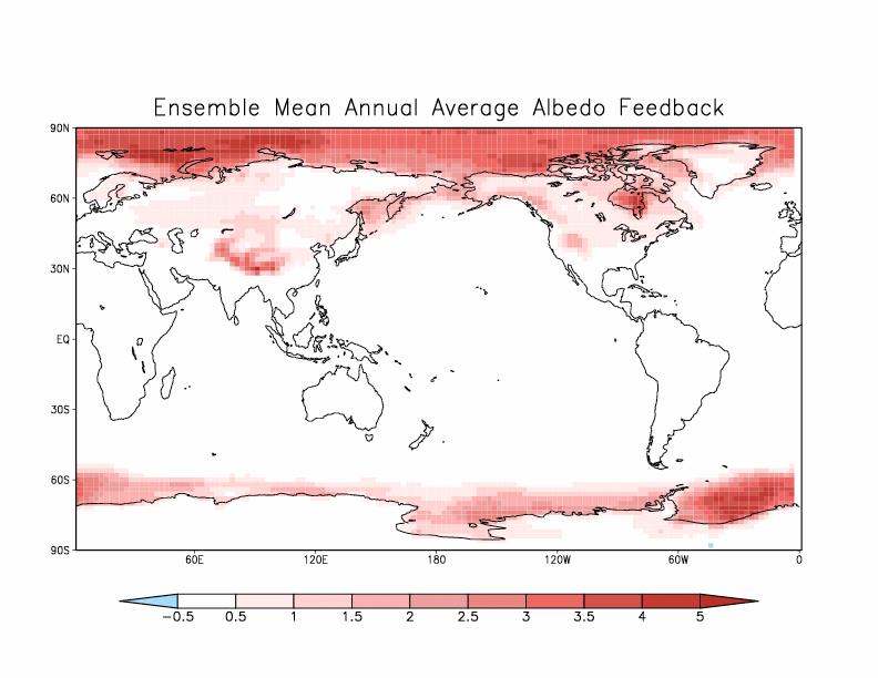
12 and 2100 ( ) are used to determine the feedbacks. To aid intermodel comparison and avoid errors due to differences in model topography, surface pressure data from GFDL CM2.0 model are used exclusively. It should be noted that the climate system is not in equilibrium at the end of the period of interest, which means that the responses used here are transient. Allen and Ingram (2002) in particular reported differences between transient and equilibrium warming patterns, but these differences are assumed to be small. b. Environmental changes Knowledge of the response of the environmental variables of interest (surface albedo, temperature, and water vapor) is necessary to understand how the radiative budget changes. The following is a discussion of the ensemble mean environmental changes in the models. Albedo is the fraction of incoming radiation that is reflected, or a = 1 (SW up / SW down ). (1) As the earth warms, its albedo decreases because snow and ice melt to reveal land, which absorbs more sunlight (Fig. 2a). There are essentially no albedo changes between 30 N and 50 S. The largest changes by far are at the poles, with the Arctic dominating over the Antarctic. All of the Arctic Ocean sees decreases in albedo of 0.04 % K -1 or greater. There is no change over most of the Antarctic continent, except for the areas east of the Ross Ice Shelf and South of the Ronne Ice Shelf. The maximum decrease in albedo in the Southern Ocean is % K -1 to 0.04 % K -1 in the Ronne Ice Shelf. Other locations that reach 0.04 % K -1 decrease in albedo are Hudson Bay and the Bering Sea. The Sea of Okhostk also sees a maximum decrease in albedo of 0.03 % K -1. Land areas that have a

13 decrease in albedo of 0.02 % K -1 to % K -1 are the western United States, Canada s Pacific coast, the Tibetan Plateau, and western Russia. The amount of water vapor in the air should increase as the surface temperature increases because evaporation occurs according to the Clausseus-Claperon equation. Changes in humidity are shown via the annual, ensemble, zonal mean of the fractional change in specific humidity per degree warming (Fig. 2b). The water vapor above 500 hpa increases by at least 10 % K -1. The maximum increase is over 30 % K -1, and it occurs between 100 and 200 hpa near the equator. There is also a change of over 20 % K -1 north of 75 N. Surface temperature is the variable most people relate to global warming, but the temperature throughout the troposphere determines the temperature feedback at the surface (e.g., Pierrehumbert 1995). The ensemble, zonal, mean temperature change per degree warming (ignoring the surface temperature change, Fig. 2c) is a maximum of 2 K K -1 at 200 hpa over the equator. Changes above this level will not be considered because this paper focuses on changes in the troposphere only, for the sake of simplicity and because the effects of the tropospheric environment on the surface radiation budget dwarf those of higher parts of the atmosphere. The temperature change at levels above 300 hpa actually becomes negative north of 60 N. There is also an increase of more than 1.5 K K -1 north of 60 N below 800 hpa. The surface temperature changes per degree global mean warming are shown in figure 2d. The minimum surface temperature changes (where there is no change) are found in the Northern Atlantic and Southern Pacific and Indian Oceans. The largest

14 changes are over the Arctic Ocean, reaching values of over 2.4 K K -1. Greater changes occur over land than ocean, and more north than south. c. Radiative adjoints In order to determine the effect of changing each of these variables on the surface radiation budget, the change in radiation at the surface due to each variable is calculated. This is not a standardized output of the AR4 models, so instead 3-hourly values from the GFDL GCM (GAMDT 2004) are used to calculate the partial derivative of the surface radiative flux with respect to each variable of interest (surface albedo, a, temperature, T, and water vapor, w). Using the terminology of Soden and Held (2005), these derivatives are called radiative adjoints (K x ). Differences in radiative algorithms are assumed to be small compared to differences in model responses as in Soden and Held (2005), allowing the same adjoints to be used for all models. Soden and Held (2005) describes the calculation of the radiative adjoints. The calculation is done in a control simulation of the GFDL GCM using values of the current climate. At each level k, the temperature is increased by 1 K and the change in the surface radiation flux determines δr/δt. To compute δr/δw, the relative humidity is held constant and the temperature used to compute the saturation mixing ratio is increased by 1 K. To compute δr/δa, the surface albedo is increased by one percent. Extensive discussion of the radiative adjoints is available in Held and Soden (2000). Annual mean radiative adjoints are shown in figure 2. For albedo we will look at the horizonal data, but for the rest we will only consider ensemble zonal means. The albedo kernels have units of energy per area per percent change in albedo. The water vapor kernels have units of energy per unit area per unit pressure; water vapor is

15 measured in dimensionless units. The temperature feedback kernel is measured in units of energy per area unit per pressure unit per temperature unit. The kernels are divided into longwave and shortwave components. The temperature kernel is only longwave and the albedo feedback only shortwave, while the water vapor feedback comprises both components. The Planck temperature response, or the change in longwave radiation with changes in temperature, is evaluated in the zonal and annual mean (Fig. 3a). It only affects the longwave range of radiation because Earth emits very little radiation in the shortwave relative to the amount it emits in the longwave or the amount the sun emits in the shortwave. The largest values, around 9 W m -2 hpa -1 K -1 are found around 1000 hpa near 60 S. Above 500 hpa the temperature adjoints vanish, and there are only two regions above 800 hpa with non-zero adjoint values: over the Antarctic and between 30 and 40 N. Over the Antarctic, adjoints reach a minimum of -1 at 700 hpa, while in the more northern region, they increase monotonically. Over the rest of the world, adjoints decrease from 7 or 8 at 1000 hpa and vanish above 850 hpa. The water vapor feedback occurs in both the long and shortwave parts of the radiation spectrum because water vapor is radiatively active in both parts of the spectrum. The longwave response is much greater than the shortwave. In the longwave zonal, annual mean (not shown), water vapor is neutral above 500 hpa. The only area where the kernel is greater than 0.3 W m -2 hpa -1 K -1 is over Antarctica. Most values are positive, below 800 hpa and between 60 N and 60 S. They increase to a maximum at the equator of 2.4 W m -2 hpa -1 K -1. The shortwave water vapor kernel vanishes above 500 hpa and poleward of about 70 N and S (not shown). It decreases to a minimum of W m -2

16 hpa -1 K -1 at 1000 hpa at the equator. Since the water vapor response is dominated by its longwave component, the net adjoint (Fig. 3b) is very similar to (but slightly smaller than) the longwave component. The Earth s albedo only impacts absorption in the shortwave; the Earth is approximately a blackbody in the longwave region (Fig. 3c). All of the polar albedo adjoint values are greater than -1 W m -2 % -1. Values less than -1 are found nearly everywhere between 30 S and 30 N, but if you recall, the albedo doesn t change in these areas. The albedo in the western US ranges from about 1 to 2 W m -2 % -1, and from about 1.4 to 0.4 W m -2 % -1 over western Russia. Kernels over the Tibetan Plateau range from 1.2 to 1.8 W m -2 % -1, and changes over the Pacific coast of Canada are between 0.6 and 0.8 W m -2 % Methodology At earth s surface, the energy balance has three components: latent heat, sensible heat, and radiation. Radiation can be separated into longwave and shortwave regions of the spectrum. The direction of propagation of radiation is important when considering the physics of climate. Radiation propagating downwards is referred to as downwelling, while radiation propagating upwards is called upwelling. The only source of shortwave radiation on Earth is the sun, so downwelling shortwave radiation is direct sunlight, while upwelling shortwave radiation is the reflected sunlight. At the surface, downwelling longwave is radiation that has been emitted by the atmosphere, while upwelling longwave is radiation emitted at the surface. As mentioned above, latent heat is the energy released by phase transformation, and the only one of concern in our atmosphere

17 is that of water. The sensible heat transfer important on climactic timescales is the ocean s heat content. At any time, this balance can be represented by S(w, I, C) L(T, w,co 2, C) = F (2) where S represents absorbed shortwave radiation (upwelling is negative, so it is upwelling minus downwelling, which is always positive) which depends on water vapor (w), ice and snow cover, (I), clouds (C), and CO 2 ; L is the net longwave radiation (downwelling minus upwelling) which depends on temperature (T), water vapor, CO 2, and clouds; and F is sum of the sensible and latent heat. R will be used to represent the net radiation, S L (upwelling is negative). As the radiation budget changes with global warming, the change in net radiation ( R) depends on the radiative forcing ( F co2 ) and feedbacks due to water vapor, ice and snow cover (we ignore land use changes, so these are represented by changes in albedo, a), temperature, and clouds, R = F = F co2 + F T + F w + F a + F C, (3) where each F x represents a radiative feedback. Take note that cloud feedbacks involve nonlinearities and thus will be dealt with separately from the rest of the feedbacks. The sign convention was chosen so that positive feedback values amplify the original perturbation and negative values diminish it. a. Calculations A feedback parameter λ x = K x dx/dt s quantifies each feedback. dx/dt s is calculated from the differences of the two climates dx/dt s = (x 2100 x 2000 ) / T s. (4) Each λ x is then vertically integrated to the tropopause and globally averaged to obtain global feedback parameters. The tropopause is defined as 100 hpa at the equator varying

18 linearly to 300 hpa at the poles. This is done for water vapor, temperature, and albedo feedbacks. The sum of the feedback parameters is a total feedback parameter of sorts, λ = λ T + λ w + λ a + λ C. (5) Each model s surface temperature response in the carbon dioxide doubling experiment is different, and this must be accounted for if the models are to be compared meaningfully. The feedback parameters accomplish this by implicitly being scaled by the surface temperature change in the model. Once the temperature, water vapor, and surface albedo feedbacks are known, as well as forcing and net changes in radiation, the cloud feedback is calculated as their residual, λ C = R/ T s λ T λ w λ a F co2 / T s. (6) The forcing is taken to be W m -2 for all models, and it is assumed to be uniform globally and for all seasons. Though this is not a precise value, the forcing term is dominated by the change in radiation and the other feedbacks, so the resulting error is assumed to be small. Because surface albedo and change in radiation are only defined at the surface, no information about the vertical structure of this feedback parameter can be obtained from this method. Four of the models (GISS E-H and E-R and NCAR CCSM3 and PCM1) do not provide radiation values, so cloud feedbacks are only calculated for the remaining ten models. The ensemble, annual mean radiative flux changes per degree warming are shown in Figure 4. The zonal mean radiative flux due to temperature change (Fig. 4a) has the largest (negative) changes at the surface. The other significant contributions are at low

19 levels north of 45 N and within 15 degrees of the equator. At 30 N, the change is spread to higher levels (as high at 600 hpa). The water vapor feedback (Fig. 4b) is positive and concentrated at low levels over the equator. It decreases from a maximum of 2.4 W m -2 hpa -1 K -1 with height and poleward movement. The feedback vanishes at the surface because in the models, the lowest level represents the actual ground, which does not contain water vapor because it is solid. The largest changes due to surface albedo (Fig. 4c) are found in the Hudson Bay, over the Tibetan Plateau, and east of Svalbard in the Arctic Ocean. The next largest changes are over the rest of the Arctic. This is no doubt due to melting of glaciers and sea ice as the planet warms. The water vapor feedback can be broken into short (Fig. 4d) and longwave components (Fig. 4e). Water vapor absorbs shortwave radiation incident from the sun before it reaches the surface, decreasing the amount of shortwave radiation reaching the surface and resulting in a negative feedback. In contrast, water vapor both absorbs longwave radiation emitted from the surface and re-emits it in all directions. Figures 4d and 4e show that the majority of the contribution comes from the longwave component, while the shortwave effects tend to counteract this, and both are at a maximum between 900 and 800 hpa in the tropics. Column integrated annual mean temperature and water vapor feedback parameters for each model, as well as the annual mean surface albedo feedback parameters, are shown and discussed in the Appendix.

20 4. Results a. Global Average Responses Global, annual mean feedback parameters for each model are shown in Figure 5. The ensemble spread for each feedback parameter is visible in Figure 5a, and it is clear that the cloud feedback is less certain than the other feedbacks (this issue will be discussed further below). Values for the primary feedbacks shown here are also in Table 3. The water vapor feedback (which is positive) dominates the albedo (also positive) and temperature (negative) feedbacks (Fig. 5b). The inverse relationship of the temperature and water vapor feedbacks in each model is noticeable. Examination of water vapor feedback (Fig. 5c) shows that almost all of the intermodel variability in this feedback results from the longwave response. When the temperature response is broken down into the parts resulting from vertically uniform and non-uniform warming (Fig. 5d), it is apparent that most of the variability in the temperature feedback is due to non-uniform warming. The models are in poor agreement on this feedback; they do not even agree on whether it is negative or positive. The inverse relationship means that the balance in the models between the temperature and water vapor feedbacks is more specifically between the longwave water vapor and differential warming feedbacks. This compensation is discussed in Zhang et al. (1994). Finally, the corresponding responses in a constant relative humidity atmosphere are compared to responses in the models (Fig. 5e). This is done by using the temperature response in the IPCC models and assuming relative humidity is constant, following Soden and Held (2005). In a constant relative humidity atmosphere, both components of the water vapor feedback are just slightly more extreme, and the constant relative

21 humidity net feedback is slightly higher than that observed in the actual model responses. Soden and Held (2005) found that the constant relative humidity response agreed to within 5% of the actual response. Here, they only agree within 15%. Comparing the data in Table 3 with that of Table 1 of Soden and Held (2005), the albedo feedback parameters are identical; water vapor feedbacks are smaller; lapse rate feedbacks are much smaller; and cloud feedbacks are much different. b. Vertical structure of feedbacks The global, annual, ensemble mean vertical structure of temperature feedback parameters and each component of the water vapor feedback parameter are shown in Figure 6. All feedback parameters vanish with increasing height, so the lower troposphere dominates the response. The shortwave water vapor feedback is always negative and the longwave water vapor feedback is always positive, but the temperature feedback changes from (very) negative at the surface to positive just above it. This is because radiation emitted at the surface can only leave the surface, so it is a negative feedback by definition. In the atmosphere, the emission of radiation is in all directions, while some radiation escapes to space, some is also reabsorbed at the surface or elsewhere in the atmosphere, resulting in a positive feedback. Plots corresponding to Figure 6 for each model can be found in the appendix. c. Cloud feedback The cloud feedback parameter and the values from which it was calculated are shown for each model in Figure 7a. The change in radiation shows far more intermodel spread than any of the water vapor, temperature, or albedo feedbacks (and all forcings are the same), so this variability is attributed to cloud feedbacks. This feedback is negative

22 in most (nine) models, but differing in degree from almost neutral to much larger than all the other feedbacks combined. The distribution of the ensemble mean, annually averaged cloud feedback is shown in figure 7b. The most extreme values, lower than -45 W m -2 K -1 (not shown), occur near mountain ranges (the Andes, and the Tibetan plateau, with less extreme values in the Rockies). On a scale similar to the temperature feedbacks, the cloud feedback is extremely variable over the continents. However, it is important to remember that the cloud feedback is calculated as a residual, so it inherits the variability of the terms used in its calcuation. 5. Discussion The information presented above is simply an analysis of the radiative portion of the surface energy budget. The importance of the total energy budget is that it constrains changes in evaporation, causing changes in circulation. This is the first study to attempt to decompose the contributions of various feedbacks in determining the response of the hydrologic cycle to increasing greenhouse gases. This paper has described some important aspects of the surface radiation budget. The next step is to consider these findings in the context of the total energy budget at the surface and its interactions with the latent and sensible heat changes. The difference between the transient and equilibrium states is especially important for the latent heat balance because the ocean changes on a much longer timescale than the atmosphere or land surface. This has important repercussions on the sensible heat balance, so experiments that run to equilibrium are necessary for this work. The effects of changes

23 of the surface energy and mass budgets on global circulation should also be explored in future work to complete the picture of how precipitation will change. No information about the vertical structure of cloud feedbacks was available for this study. As a result, there is no information about the types of clouds causing this feedback, which is very important to understanding the feedback and climate change in general. For more information on cloud feedbacks, see Bony et al. (2004). 6. Conclusions Most of the temperature and water vapor feedbacks occur at the lowest levels of the atmosphere. The main contribution of the surface albedo feedback is near the poles, especially the Arctic, while the main contribution of the water vapor feedback is from the tropics. Contributions from all latitudes are important for the temperature feedback. Corresponding to the findings of Soden and Held (2005) for the TOA, the cloud feedback at the surface has the most intermodel variability (thus uncertainty) of all of the feedbacks, and, perhaps, magnitude. And water vapor provides the largest positive feedback. There is a compensation between longwave water vapor and differential warming feedbacks that reduces differences in climate sensitivies among models.

24 FIGURES Figure 1. Atmospheric water vapor change (%) as a function of temperature change (K) is shown (a) for twelve of the models used with a 7.5% K -1 increase predicted by the Clausius-Clapeyron equation shown for reference. Precipitation (%) versus temperature change (K) is shown (b) with the same reference line. Net surface radiative change (W m -2 ) versus precipitation change (scaled by the latent heat of vaporization, W m -2 ) is shown (c), with a regression line for reference. 1a Water vapor versus temperature Vertically Integrated Water Vapor Change (%) Temperature Change (K) 7.5%/K

25 1b Precipitation versus temperature Precip change (%) %/K Temperature Change (K) 1c Radiation v Precipitation 6 5 Change in Radiation (W/m2) Regression Line Precipitation Change * Lv (W/m2)

26 Figure 2. Ensemble, annual mean changes per degree warming over the 21 st century in surface albedo (a, % K -1 ), percent change in specific humidity (b, % K -1 ), zonal mean temperature change (c, K K -1 ), and surface temperature (d, K K -1 ). 2a 2b

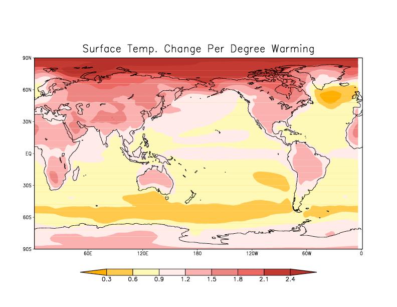
27 2c 2d

28 Figure 3. Zonal, annual mean partial derivatives of radiative flux with respect to temperature (a, W m -2 hpa -1 K -1 ), water vapor (b, W m -2 hpa -1 ), and surface albedo (c, W m -2 % -1 ). The annual mean of the derivative with respect to surface albedo is part (d, W m -2 % -1 ). 3a

29 3b

30 3c 3d

31 Figure 4. Zonal and annually averaged ensemble mean radiative flux changes per degree warming over the 21 st century due to (a) temperature, and (b) water vapor feedbacks (W m -2 hpa -1 K -1 ). Annually averaged ensemble mean radiative flux change per degree warming due to surface albedo is shown in (c, W m -2 K -1 ). The changes due to water vapor are further broken into longwave (d) and shortwave (e) components (W m -2 hpa -1 K -1 ). 4a

32 4b 4c

33 4d

34 4e

35 Figure 5. Intermodel comparison of globally, seasonally averaged feedback parameters (W m -2 K -1 ). All parameters, including their components, are compared in (a). Only the three feedbacks directly calculated here (surface albedo, temperature, and water vapor) are compared (b). The total water vapor feedback is broken into its components in (c). The temperature feedback is broken into uniform warming and changes in lapse rate in (d). Water vapor components in the models are compared with values for an atmosphere of constant relative humidity (e). 5a W/m2/K Global mean feedback parameters a t q lw q sw q tl cloud CNRM GFDL CM2.0 GFDL CM2.1 GISS AOM GISS E-H GISS E-R INMCM3 IPSL MIROC 3.2 medres MRI MPI ECHAM5 NCAR CCSM3 NCAR PCM1 UKMO HadCM3-1 -2

36 5b Primary feedbacks W/m2/K CNRM GFDL CM2.0 GFDL CM2.1 GISS AOM GISS E-H GISS E-R INM CM3 IPSL MIROC 3.2 medres MRI MPI ECHAM5 NCAR CCSM3 NCAR PCM1 Albedo Temperature Water Vapor Models

37 5c Water Vapor Feedback W/m2/K Total LW SW CNRM GFDL CM2.0 GFDL CM2.1 GISS AOM GISS E-H GISS E-R INM CM3 IPSL MIROC 3.2 medres MRI MPI ECHAM5 NCAR CCSM3 NCAR PCM1 UKMO HadCM3 Models

38 5d Temperature Feedback W/m2/K CNRM GFDL CM2.0 GFDL CM2.1 GISS AOM GISS E-H Total temperature feedback Lapse Rate Change Uniform Warming GISS E-R INM CM3 IPSL MIROC 3.2 medres Models MRI MPI ECHAM5 NCAR CCSM3 NCAR PCM1 UKMO HadCM3

39 5e Water Vapor Feedback for Constant and Varying RH W/m2/K CNRM GFDL CM2.0 GFDL CM2.1 GISS AOM GISS E-H GISS E-R INM CM3 IPSL MIROC 3.2 medres Models MRI MPI ECHAM5 NCAR CCSM3 NCAR PCM1 UKMO HadCM3 SW Constant RH LW Constant RH LW SW Total, Constant RH Total

40 Figure 6. Vertical structure of globally, annually averaged ensemble mean feedback parameters (W m -2 hpa -1 K -1 ). Surface albedo feedback is indicated by an arrow (W m -2 K -1 ). 6

41 Figure 7. Intermodel comparison of globally, seasonally averaged feedback parameters and net radiative change per degree warming (a, W m -2 K -1 ). Ensemble mean, annually averaged cloud feedback (b, W m -2 K -1 ). 7a Cloud feedback W/m2/K CNRM GFDL CM2.0 GFDL CM2.1 GISS AOM INM CM3 IPSL MIROC 3.2 medres MRI MPI ECHAM5 UKMO HadCM3 Cloud feedback dr/dt forcing/dt Albedo feedback Temperature feedback Water Vapor feedback Models

42 7b