For GLM y = Xβ + e (1) where X is a N k design matrix and p(e) = N(0, σ 2 I N ), we can estimate the coefficients from the normal equations
|
|
|
- Reynold Watkins
- 5 years ago
- Views:
Transcription
1 1 Generalised Inverse For GLM y = Xβ + e (1) where X is a N k design matrix and p(e) = N(0, σ 2 I N ), we can estimate the coefficients from the normal equations (X T X)β = X T y (2) If rank of X, denoted r(x), is k (ie. full rank) then X T X has an inverse (it is nonsingular ) and ˆβ = (X T X) 1 X T y (3) But if r(x) < k we can have Xβ 1 = Xβ 2 (ie. same predictions) with β 1 β 2 (different parameters). The parameters are then not therefore unique, identifiable or estimable. For example, a design matrix sometimes used in the 1
2 Analysis of Variance (ANOVA) X = (4) has k = 3 columns but rank r(x) = 2 ie. only two linearly independent columns (any column can be expressed as a linear combination of the other two). For models such as these X T X is not invertible, so we must resort to the generalised inverse, X. This is defined as any matrix X such that XX X = X. It can be shown that in the general case ˆβ = (X T X) X T y (5) = X y If X is full-rank, X T X is invertible and X = (X T X) 1 X T. 2
3 There are many generalise inverses. We would often choose the pseudo-inverse (pinv in MATLAB) ˆβ = X + y (6) Take home message: avoid rank-deficient designs. If X is full rank, then X + = X = (X T X) 1 X T. 2 Estimating error variance An unbiased estimate for the error variance σ 2 can be derived as follows. Let where P is the projection matrix X ˆβ = P y (7) P = X(X T X) X T (8) = XX P y projects the data y into the space of X. P has two important properties (i) it is symmetric P T = P, (ii) 3
4 P P =P. This second property follows from it being a projection. If what is being projected is already in X space (ie. P y) then looking for that component of it that is in X space will give the same thing ie. P P y = P y. Then residuals are ê = y X ˆβ (9) = (I P )y = Ry where R = I N XX is the residual-forming matrix. Remember, ê is that component of the data, orthogonal to the space X. Ry is another projection matrix, but one that projects the data y into the orthogonal complement of X. Similarly, R has the two properties (i) R T = R and (ii) RR = R. We now look seek an unbiased estimator of the variance by first looking at the expected sum of squares E[ê T ê] = E[y T R T Ry] (10) = E[y T Ry] 4
5 5
6 We now use the standard result: If p(a) = N(µ, V ) then E[a T Ba] = µ T Bµ + T r(bv ) So, if p(y) = N(X ˆβ, σ 2 I N ) then E[y T Ry] = ˆβ T X T RX ˆβ + T r(σ 2 R) (11) = ˆβ T (X T X X T XX X) ˆβ + T r(σ 2 R) = T r(σ 2 (I P )) = σ 2 (N r(p )) = σ 2 (N k) So, an unbiased estimate of the variance is ˆσ 2 = (y T Ry)/(N k) (12) = RSS/(N k) where the RSS is Residual Sum of Squares. Remember, 6
7 the ML variance estimate is ˆσ 2 ML = (y T Ry)/N (13) 3 Comparing nested GLMs Full model: Reduced model: Consider the test-statistic y = X 0 β 0 + X 1 β 1 + e (14) y = X 0 β 0 + e 0 (15) f = (RSS red RSS full )/(k p) RSS full /(N k) where Residual Sum of Squares (RSS) are (16) RSS full = ê T ê (17) RSS red = ê T 0 ê 0 (18) 7
8 We can re-write in terms of Extra Sum of Squares where f = ESS/(k p) RSS full /(N k) (19) ESS = RSS red RSS full (20) We can compute these quantities using RSS full = y T Ry (21) RSS red = y T R 0 y We expect the denominator to be E[RSS full /(N k)] = σ 2 (22) and, under the null (β 1 = 0), we have σ 2 0 = σ 2 and therefore expect the numerator to be E[(RSS red RSS full )/(k p)] = σ 2 (23) where r(r 0 R) = k p (mirroring the earlier expectation calculation). Under the null, we therefore expect a 8
9 test statistic of unity < f >= σ2 σ 2 (24) as both numerator and denominator are unbiased estimates of error variance. We might naively expect to get a numerator of zero, under the null. But this is not the case because, in any finite sample, ESS will be non zero. When we then divide by (k p) we get E[ESS/(k p)] = σ 2. When the full model is better we get a larger f value. 4 Partial correlation and R 2 The square of the partial correlaton coefficient R 2 y,x 1 X 0 = RSS red RSS full RSS red (25) is the (square) of the correlation between y and X 1 β 1 after controlling for the effect of X 0 β 0. Abbreviating the 9
10 above to R 2, the F-statistic can be re-written as f = R 2 /(k p) (1 R 2 )/(N k) (26) Model comparison tests are identical to tests of partial correlation. In X 0 explains no variance eg. it is a constant or empty matrix then R 2 = Y T Y Y T RY (27) Y T Y which is the proportion of variance explained by the model with design matrix X. More generally, if X 0 is not the empty matrix then R 2 is that proportion of the variability unexplained by the reduced model X 0 that is explained by the full model X. 5 Examples 10
11 11
12 12
13 13
14 14
15 15
16 16
17 6 How large must f be for a significant improvement? Under the null (β 1 = 0), f follows an F -distribution with k p numerator degrees of freedom (DF) and N k denominator DF. Info on PDFs and transforming them. 17
18 7 Contrasts We can also compare nested models using contrasts. This is more efficient, as we only need to estimate parameters of the full model. For a contrast matrix C we wish to test the hypothesis C T β = 0. This can correspond to a model comparison, as before, if C is chosen appropriately. But it is also more general, as we can test any effect which can be expressed as C T β = H T Xβ (28) for some H. This defines a space of estimable contrasts. The contrast C defines a subspace X c = XC. As before, we can think of the hypothesis C T β = 0 as comparing a full model, X, versus a reduced model which is now given by X 0 = XC 0 where C 0 is a contrast orthogonal to C ie. C 0 = I k CC (29) A test statistic can then be generated as before where 18
19 R 0 = I N X 0 X 0, M = R 0 R and f = yt My/r(M) y T Ry/r(R) (30) In fmri, the use of contrasts allows us to test for (i) main effects and interactions in factorial designs, (ii) choice of hemodynamic basis sets. Importantly, we do not need to refit models. The numerator can be calculated efficiently as y T My = ĉ T [ C T (X T X) C ] ĉ (31) where ĉ = C T ˆβ is the estimated effect size. See Christensen [1] for details. 19
20 8 Hemodynamic basis functions If C(t, u) is the Canonical basis function for event offset u then, using a first-order Taylor series approximation dc(t, u) C(t, u 0 + h) C(t, u 0 ) + h du C(t, u 0 ) + hd(t, u 0 ) (32) where the derivative is evaluated at u = u 0. This will allow us to accomodate small errors in event timings, or earlier/later rises in the hemodynamic response. 20
21 21
22 22
23 23
24 24
25 25
26 26
27 9 References [1] R. Christensen. Plane Answers to Complex Questions: The Theory of Linear Models. Springer, New York,
11 Hypothesis Testing
 28 11 Hypothesis Testing 111 Introduction Suppose we want to test the hypothesis: H : A q p β p 1 q 1 In terms of the rows of A this can be written as a 1 a q β, ie a i β for each row of A (here a i denotes
Lecture 15. Hypothesis testing in the linear model
 14. Lecture 15. Hypothesis testing in the linear model Lecture 15. Hypothesis testing in the linear model 1 (1 1) Preliminary lemma 15. Hypothesis testing in the linear model 15.1. Preliminary lemma Lemma
MA 575 Linear Models: Cedric E. Ginestet, Boston University Midterm Review Week 7
 MA 575 Linear Models: Cedric E. Ginestet, Boston University Midterm Review Week 7 1 Random Vectors Let a 0 and y be n 1 vectors, and let A be an n n matrix. Here, a 0 and A are non-random, whereas y is
Multiple Linear Regression
 Multiple Linear Regression Simple linear regression tries to fit a simple line between two variables Y and X. If X is linearly related to Y this explains some of the variability in Y. In most cases, there
This model of the conditional expectation is linear in the parameters. A more practical and relaxed attitude towards linear regression is to say that
 Linear Regression For (X, Y ) a pair of random variables with values in R p R we assume that E(Y X) = β 0 + with β R p+1. p X j β j = (1, X T )β j=1 This model of the conditional expectation is linear
Ch 3: Multiple Linear Regression
 Ch 3: Multiple Linear Regression 1. Multiple Linear Regression Model Multiple regression model has more than one regressor. For example, we have one response variable and two regressor variables: 1. delivery
Statistical Inference
 Statistical Inference J. Daunizeau Institute of Empirical Research in Economics, Zurich, Switzerland Brain and Spine Institute, Paris, France SPM Course Edinburgh, April 2011 Image time-series Spatial
[y i α βx i ] 2 (2) Q = i=1
![[y i α βx i ] 2 (2) Q = i=1](/thumbs/75/72005858.jpg "[y i α βx i ] 2 (2) Q = i=1") Least squares fits This section has no probability in it. There are no random variables. We are given n points (x i, y i ) and want to find the equation of the line that best fits them. We take the equation
Least squares fits This section has no probability in it. There are no random variables. We are given n points (x i, y i ) and want to find the equation of the line that best fits them. We take the equation
3. For a given dataset and linear model, what do you think is true about least squares estimates? Is Ŷ always unique? Yes. Is ˆβ always unique? No.
 7. LEAST SQUARES ESTIMATION 1 EXERCISE: Least-Squares Estimation and Uniqueness of Estimates 1. For n real numbers a 1,...,a n, what value of a minimizes the sum of squared distances from a to each of
Statistical Inference
 Statistical Inference Jean Daunizeau Wellcome rust Centre for Neuroimaging University College London SPM Course Edinburgh, April 2010 Image time-series Spatial filter Design matrix Statistical Parametric
Linear Models Review
 Linear Models Review Vectors in IR n will be written as ordered n-tuples which are understood to be column vectors, or n 1 matrices. A vector variable will be indicted with bold face, and the prime sign
Peter Hoff Linear and multilinear models April 3, GLS for multivariate regression 5. 3 Covariance estimation for the GLM 8
 Contents 1 Linear model 1 2 GLS for multivariate regression 5 3 Covariance estimation for the GLM 8 4 Testing the GLH 11 A reference for some of this material can be found somewhere. 1 Linear model Recall
The linear model is the most fundamental of all serious statistical models encompassing:
 Linear Regression Models: A Bayesian perspective Ingredients of a linear model include an n 1 response vector y = (y 1,..., y n ) T and an n p design matrix (e.g. including regressors) X = [x 1,..., x
Estimable Functions and Their Least Squares Estimators. Copyright c 2012 Dan Nettleton (Iowa State University) Statistics / 51
 Statistics / 51") Estimable Functions and Their Least Squares Estimators Copyright c 2012 Dan Nettleton (Iowa State University) Statistics 611 1 / 51 Consider the GLM y = n p X β + ε, where E(ε) = 0. p 1 n 1 n 1 Suppose
Estimable Functions and Their Least Squares Estimators Copyright c 2012 Dan Nettleton (Iowa State University) Statistics 611 1 / 51 Consider the GLM y = n p X β + ε, where E(ε) = 0. p 1 n 1 n 1 Suppose
Associated Hypotheses in Linear Models for Unbalanced Data
 University of Wisconsin Milwaukee UWM Digital Commons Theses and Dissertations May 5 Associated Hypotheses in Linear Models for Unbalanced Data Carlos J. Soto University of Wisconsin-Milwaukee Follow this
Linear Regression. In this problem sheet, we consider the problem of linear regression with p predictors and one intercept,
 Linear Regression In this problem sheet, we consider the problem of linear regression with p predictors and one intercept, y = Xβ + ɛ, where y t = (y 1,..., y n ) is the column vector of target values,
Ch 2: Simple Linear Regression
 Ch 2: Simple Linear Regression 1. Simple Linear Regression Model A simple regression model with a single regressor x is y = β 0 + β 1 x + ɛ, where we assume that the error ɛ is independent random component
Quick Review on Linear Multiple Regression
 Quick Review on Linear Multiple Regression Mei-Yuan Chen Department of Finance National Chung Hsing University March 6, 2007 Introduction for Conditional Mean Modeling Suppose random variables Y, X 1,
4 Multiple Linear Regression
 4 Multiple Linear Regression 4. The Model Definition 4.. random variable Y fits a Multiple Linear Regression Model, iff there exist β, β,..., β k R so that for all (x, x 2,..., x k ) R k where ε N (, σ
1 Least Squares Estimation - multiple regression.
 Introduction to multiple regression. Fall 2010 1 Least Squares Estimation - multiple regression. Let y = {y 1,, y n } be a n 1 vector of dependent variable observations. Let β = {β 0, β 1 } be the 2 1
Maximum Likelihood Estimation
 Maximum Likelihood Estimation Merlise Clyde STA721 Linear Models Duke University August 31, 2017 Outline Topics Likelihood Function Projections Maximum Likelihood Estimates Readings: Christensen Chapter
Chapter 3: Multiple Regression. August 14, 2018
 Chapter 3: Multiple Regression August 14, 2018 1 The multiple linear regression model The model y = β 0 +β 1 x 1 + +β k x k +ǫ (1) is called a multiple linear regression model with k regressors. The parametersβ
The General Linear Model (GLM)
") he General Linear Model (GLM) Klaas Enno Stephan ranslational Neuromodeling Unit (NU) Institute for Biomedical Engineering University of Zurich & EH Zurich Wellcome rust Centre for Neuroimaging Institute
he General Linear Model (GLM) Klaas Enno Stephan ranslational Neuromodeling Unit (NU) Institute for Biomedical Engineering University of Zurich & EH Zurich Wellcome rust Centre for Neuroimaging Institute
CAS MA575 Linear Models
 CAS MA575 Linear Models Boston University, Fall 2013 Midterm Exam (Correction) Instructor: Cedric Ginestet Date: 22 Oct 2013. Maximal Score: 200pts. Please Note: You will only be graded on work and answers
14 Multiple Linear Regression
 B.Sc./Cert./M.Sc. Qualif. - Statistics: Theory and Practice 14 Multiple Linear Regression 14.1 The multiple linear regression model In simple linear regression, the response variable y is expressed in
The General Linear Model. How we re approaching the GLM. What you ll get out of this 8/11/16
 8// The General Linear Model Monday, Lecture Jeanette Mumford University of Wisconsin - Madison How we re approaching the GLM Regression for behavioral data Without using matrices Understand least squares
Biostatistics 533 Classical Theory of Linear Models Spring 2007 Final Exam. Please choose ONE of the following options.
 1 Biostatistics 533 Classical Theory of Linear Models Spring 2007 Final Exam Name: Problems do not have equal value and some problems will take more time than others. Spend your time wisely. You do not
3. The F Test for Comparing Reduced vs. Full Models. opyright c 2018 Dan Nettleton (Iowa State University) 3. Statistics / 43
 3. Statistics / 43") 3. The F Test for Comparing Reduced vs. Full Models opyright c 2018 Dan Nettleton (Iowa State University) 3. Statistics 510 1 / 43 Assume the Gauss-Markov Model with normal errors: y = Xβ + ɛ, ɛ N(0, σ
3. The F Test for Comparing Reduced vs. Full Models opyright c 2018 Dan Nettleton (Iowa State University) 3. Statistics 510 1 / 43 Assume the Gauss-Markov Model with normal errors: y = Xβ + ɛ, ɛ N(0, σ
Inverse of a Square Matrix. For an N N square matrix A, the inverse of A, 1
 Inverse of a Square Matrix For an N N square matrix A, the inverse of A, 1 A, exists if and only if A is of full rank, i.e., if and only if no column of A is a linear combination 1 of the others. A is
MLES & Multivariate Normal Theory
 Merlise Clyde September 6, 2016 Outline Expectations of Quadratic Forms Distribution Linear Transformations Distribution of estimates under normality Properties of MLE s Recap Ŷ = ˆµ is an unbiased estimate
Ma 3/103: Lecture 24 Linear Regression I: Estimation
 Ma 3/103: Lecture 24 Linear Regression I: Estimation March 3, 2017 KC Border Linear Regression I March 3, 2017 1 / 32 Regression analysis Regression analysis Estimate and test E(Y X) = f (X). f is the
Signal Processing for Functional Brain Imaging: General Linear Model (2)
") Signal Processing for Functional Brain Imaging: General Linear Model (2) Maria Giulia Preti, Dimitri Van De Ville Medical Image Processing Lab, EPFL/UniGE http://miplab.epfl.ch/teaching/micro-513/ March
Signal Processing for Functional Brain Imaging: General Linear Model (2) Maria Giulia Preti, Dimitri Van De Ville Medical Image Processing Lab, EPFL/UniGE http://miplab.epfl.ch/teaching/micro-513/ March
Biostatistics 533 Classical Theory of Linear Models Spring 2007 Final Exam. Please choose ONE of the following options.
 1 Biostatistics 533 Classical Theory of Linear Models Spring 2007 Final Exam Name: KEY Problems do not have equal value and some problems will take more time than others. Spend your time wisely. You do
A Note on UMPI F Tests
 A Note on UMPI F Tests Ronald Christensen Professor of Statistics Department of Mathematics and Statistics University of New Mexico May 22, 2015 Abstract We examine the transformations necessary for establishing
F3: Classical normal linear rgression model distribution, interval estimation and hypothesis testing
 F3: Classical normal linear rgression model distribution, interval estimation and hypothesis testing Feng Li Department of Statistics, Stockholm University What we have learned last time... 1 Estimating
Appendix A: Review of the General Linear Model
 Appendix A: Review of the General Linear Model The generallinear modelis an important toolin many fmri data analyses. As the name general suggests, this model can be used for many different types of analyses,
Economics 620, Lecture 5: exp
 1 Economics 620, Lecture 5: The K-Variable Linear Model II Third assumption (Normality): y; q(x; 2 I N ) 1 ) p(y) = (2 2 ) exp (N=2) 1 2 2(y X)0 (y X) where N is the sample size. The log likelihood function
Lecture 3: Multiple Regression
 Lecture 3: Multiple Regression R.G. Pierse 1 The General Linear Model Suppose that we have k explanatory variables Y i = β 1 + β X i + β 3 X 3i + + β k X ki + u i, i = 1,, n (1.1) or Y i = β j X ji + u
Stat/F&W Ecol/Hort 572 Review Points Ané, Spring 2010
 1 Linear models Y = Xβ + ɛ with ɛ N (0, σ 2 e) or Y N (Xβ, σ 2 e) where the model matrix X contains the information on predictors and β includes all coefficients (intercept, slope(s) etc.). 1. Number of
Sampling Distributions
 Merlise Clyde Duke University September 3, 2015 Outline Topics Normal Theory Chi-squared Distributions Student t Distributions Readings: Christensen Apendix C, Chapter 1-2 Prostate Example > library(lasso2);
The outline for Unit 3
 The outline for Unit 3 Unit 1. Introduction: The regression model. Unit 2. Estimation principles. Unit 3: Hypothesis testing principles. 3.1 Wald test. 3.2 Lagrange Multiplier. 3.3 Likelihood Ratio Test.
STAT 401A - Statistical Methods for Research Workers
 STAT 401A - Statistical Methods for Research Workers One-way ANOVA Jarad Niemi (Dr. J) Iowa State University last updated: October 10, 2014 Jarad Niemi (Iowa State) One-way ANOVA October 10, 2014 1 / 39
18.S096 Problem Set 3 Fall 2013 Regression Analysis Due Date: 10/8/2013
 18.S096 Problem Set 3 Fall 013 Regression Analysis Due Date: 10/8/013 he Projection( Hat ) Matrix and Case Influence/Leverage Recall the setup for a linear regression model y = Xβ + ɛ where y and ɛ are
COS513: FOUNDATIONS OF PROBABILISTIC MODELS LECTURE 9: LINEAR REGRESSION
 COS513: FOUNDATIONS OF PROBABILISTIC MODELS LECTURE 9: LINEAR REGRESSION SEAN GERRISH AND CHONG WANG 1. WAYS OF ORGANIZING MODELS In probabilistic modeling, there are several ways of organizing models:
Bayesian Linear Models
 Bayesian Linear Models Sudipto Banerjee 1 and Andrew O. Finley 2 1 Department of Forestry & Department of Geography, Michigan State University, Lansing Michigan, U.S.A. 2 Biostatistics, School of Public
Empirical Economic Research, Part II
 Based on the text book by Ramanathan: Introductory Econometrics Robert M. Kunst robert.kunst@univie.ac.at University of Vienna and Institute for Advanced Studies Vienna December 7, 2011 Outline Introduction
Ma 3/103: Lecture 25 Linear Regression II: Hypothesis Testing and ANOVA
 Ma 3/103: Lecture 25 Linear Regression II: Hypothesis Testing and ANOVA March 6, 2017 KC Border Linear Regression II March 6, 2017 1 / 44 1 OLS estimator 2 Restricted regression 3 Errors in variables 4
Linear models and their mathematical foundations: Simple linear regression
 Linear models and their mathematical foundations: Simple linear regression Steffen Unkel Department of Medical Statistics University Medical Center Göttingen, Germany Winter term 2018/19 1/21 Introduction
STAT763: Applied Regression Analysis. Multiple linear regression. 4.4 Hypothesis testing
 STAT763: Applied Regression Analysis Multiple linear regression 4.4 Hypothesis testing Chunsheng Ma E-mail: cma@math.wichita.edu 4.4.1 Significance of regression Null hypothesis (Test whether all β j =
AMS-207: Bayesian Statistics
 Linear Regression How does a quantity y, vary as a function of another quantity, or vector of quantities x? We are interested in p(y θ, x) under a model in which n observations (x i, y i ) are exchangeable.
Economics 573 Problem Set 5 Fall 2002 Due: 4 October b. The sample mean converges in probability to the population mean.
 Economics 573 Problem Set 5 Fall 00 Due: 4 October 00 1. In random sampling from any population with E(X) = and Var(X) =, show (using Chebyshev's inequality) that sample mean converges in probability to..
Bayesian Linear Models
 Bayesian Linear Models Sudipto Banerjee 1 and Andrew O. Finley 2 1 Biostatistics, School of Public Health, University of Minnesota, Minneapolis, Minnesota, U.S.A. 2 Department of Forestry & Department
BIOS 2083 Linear Models c Abdus S. Wahed
 Chapter 5 206 Chapter 6 General Linear Model: Statistical Inference 6.1 Introduction So far we have discussed formulation of linear models (Chapter 1), estimability of parameters in a linear model (Chapter
2.7 Estimation with linear Restriction
 Proof (Method 1: show that that a C(W T ), which implies that the GLSE is an estimable function under the old model is also an estimable function under the new model; secnd show that E[a T ˆβ G ] = a T
Economics 620, Lecture 4: The K-Variable Linear Model I. y 1 = + x 1 + " 1 y 2 = + x 2 + " 2 :::::::: :::::::: y N = + x N + " N
 1 Economics 620, Lecture 4: The K-Variable Linear Model I Consider the system y 1 = + x 1 + " 1 y 2 = + x 2 + " 2 :::::::: :::::::: y N = + x N + " N or in matrix form y = X + " where y is N 1, X is N
MFin Econometrics I Session 4: t-distribution, Simple Linear Regression, OLS assumptions and properties of OLS estimators
 MFin Econometrics I Session 4: t-distribution, Simple Linear Regression, OLS assumptions and properties of OLS estimators Thilo Klein University of Cambridge Judge Business School Session 4: Linear regression,
Regression. ECO 312 Fall 2013 Chris Sims. January 12, 2014
 ECO 312 Fall 2013 Chris Sims Regression January 12, 2014 c 2014 by Christopher A. Sims. This document is licensed under the Creative Commons Attribution-NonCommercial-ShareAlike 3.0 Unported License What
3 Multiple Linear Regression
 3 Multiple Linear Regression 3.1 The Model Essentially, all models are wrong, but some are useful. Quote by George E.P. Box. Models are supposed to be exact descriptions of the population, but that is
The General Linear Model. Monday, Lecture 2 Jeanette Mumford University of Wisconsin - Madison
 The General Linear Model Monday, Lecture 2 Jeanette Mumford University of Wisconsin - Madison How we re approaching the GLM Regression for behavioral data Without using matrices Understand least squares
Brief Suggested Solutions
 DEPARTMENT OF ECONOMICS UNIVERSITY OF VICTORIA ECONOMICS 366: ECONOMETRICS II SPRING TERM 5: ASSIGNMENT TWO Brief Suggested Solutions Question One: Consider the classical T-observation, K-regressor linear
Sampling Distributions
 Merlise Clyde Duke University September 8, 2016 Outline Topics Normal Theory Chi-squared Distributions Student t Distributions Readings: Christensen Apendix C, Chapter 1-2 Prostate Example > library(lasso2);
One-Way ANOVA Model. group 1 y 11, y 12 y 13 y 1n1. group 2 y 21, y 22 y 2n2. group g y g1, y g2, y gng. g is # of groups,
 One-Way ANOVA Model group 1 y 11, y 12 y 13 y 1n1 group 2 y 21, y 22 y 2n2 group g y g1, y g2, y gng g is # of groups, n i denotes # of obs in the i-th group, and the total sample size n = g i=1 n i. 1
Simple and Multiple Linear Regression
 Sta. 113 Chapter 12 and 13 of Devore March 12, 2010 Table of contents 1 Simple Linear Regression 2 Model Simple Linear Regression A simple linear regression model is given by Y = β 0 + β 1 x + ɛ where
Statistical Distribution Assumptions of General Linear Models
 Statistical Distribution Assumptions of General Linear Models Applied Multilevel Models for Cross Sectional Data Lecture 4 ICPSR Summer Workshop University of Colorado Boulder Lecture 4: Statistical Distributions
Basic Distributional Assumptions of the Linear Model: 1. The errors are unbiased: E[ε] = The errors are uncorrelated with common variance:
![Basic Distributional Assumptions of the Linear Model: 1. The errors are unbiased: E[ε] = The errors are uncorrelated with common variance:](/thumbs/95/122989574.jpg "Basic Distributional Assumptions of the Linear Model: 1. The errors are unbiased: E[ε] = The errors are uncorrelated with common variance:") 8. PROPERTIES OF LEAST SQUARES ESTIMATES 1 Basic Distributional Assumptions of the Linear Model: 1. The errors are unbiased: E[ε] = 0. 2. The errors are uncorrelated with common variance: These assumptions
8. PROPERTIES OF LEAST SQUARES ESTIMATES 1 Basic Distributional Assumptions of the Linear Model: 1. The errors are unbiased: E[ε] = 0. 2. The errors are uncorrelated with common variance: These assumptions
Statistics II Exercises Chapter 5
 Statistics II Exercises Chapter 5 1. Consider the four datasets provided in the transparencies for Chapter 5 (section 5.1) (a) Check that all four datasets generate exactly the same LS linear regression
Estimating σ 2. We can do simple prediction of Y and estimation of the mean of Y at any value of X.
 Estimating σ 2 We can do simple prediction of Y and estimation of the mean of Y at any value of X. To perform inferences about our regression line, we must estimate σ 2, the variance of the error term.
The Standard Linear Model: Hypothesis Testing
 Department of Mathematics Ma 3/103 KC Border Introduction to Probability and Statistics Winter 2017 Lecture 25: The Standard Linear Model: Hypothesis Testing Relevant textbook passages: Larsen Marx [4]:
Multivariate Regression
 Multivariate Regression The so-called supervised learning problem is the following: we want to approximate the random variable Y with an appropriate function of the random variables X 1,..., X p with the
First Year Examination Department of Statistics, University of Florida
 First Year Examination Department of Statistics, University of Florida August 20, 2009, 8:00 am - 2:00 noon Instructions:. You have four hours to answer questions in this examination. 2. You must show
The General Linear Model in Functional MRI
 The General Linear Model in Functional MRI Henrik BW Larsson Functional Imaging Unit, Glostrup Hospital University of Copenhagen Part I 1 2 Preface The General Linear Model (GLM) or multiple regression
Chapter 8: Hypothesis Testing Lecture 9: Likelihood ratio tests
 Chapter 8: Hypothesis Testing Lecture 9: Likelihood ratio tests Throughout this chapter we consider a sample X taken from a population indexed by θ Θ R k. Instead of estimating the unknown parameter, we
Categorical Predictor Variables
 Categorical Predictor Variables We often wish to use categorical (or qualitative) variables as covariates in a regression model. For binary variables (taking on only 2 values, e.g. sex), it is relatively
Review of Classical Least Squares. James L. Powell Department of Economics University of California, Berkeley
 Review of Classical Least Squares James L. Powell Department of Economics University of California, Berkeley The Classical Linear Model The object of least squares regression methods is to model and estimate
ECON 5350 Class Notes Functional Form and Structural Change
 ECON 5350 Class Notes Functional Form and Structural Change 1 Introduction Although OLS is considered a linear estimator, it does not mean that the relationship between Y and X needs to be linear. In this
Simple Linear Regression
 Simple Linear Regression ST 430/514 Recall: A regression model describes how a dependent variable (or response) Y is affected, on average, by one or more independent variables (or factors, or covariates)
2. Regression Review
 2. Regression Review 2.1 The Regression Model The general form of the regression model y t = f(x t, β) + ε t where x t = (x t1,, x tp ), β = (β 1,..., β m ). ε t is a random variable, Eε t = 0, Var(ε t
General Linear Model: Statistical Inference
 Chapter 6 General Linear Model: Statistical Inference 6.1 Introduction So far we have discussed formulation of linear models (Chapter 1), estimability of parameters in a linear model (Chapter 4), least
5.1 Consistency of least squares estimates. We begin with a few consistency results that stand on their own and do not depend on normality.
 88 Chapter 5 Distribution Theory In this chapter, we summarize the distributions related to the normal distribution that occur in linear models. Before turning to this general problem that assumes normal
ML and REML Variance Component Estimation. Copyright c 2012 Dan Nettleton (Iowa State University) Statistics / 58
 Statistics / 58") ML and REML Variance Component Estimation Copyright c 2012 Dan Nettleton (Iowa State University) Statistics 611 1 / 58 Suppose y = Xβ + ε, where ε N(0, Σ) for some positive definite, symmetric matrix Σ.
ML and REML Variance Component Estimation Copyright c 2012 Dan Nettleton (Iowa State University) Statistics 611 1 / 58 Suppose y = Xβ + ε, where ε N(0, Σ) for some positive definite, symmetric matrix Σ.
8. Hypothesis Testing
 FE661 - Statistical Methods for Financial Engineering 8. Hypothesis Testing Jitkomut Songsiri introduction Wald test likelihood-based tests significance test for linear regression 8-1 Introduction elements
Basis Penalty Smoothers. Simon Wood Mathematical Sciences, University of Bath, U.K.
 Basis Penalty Smoothers Simon Wood Mathematical Sciences, University of Bath, U.K. Estimating functions It is sometimes useful to estimate smooth functions from data, without being too precise about the
20.1. Balanced One-Way Classification Cell means parametrization: ε 1. ε I. + ˆɛ 2 ij =
 20. ONE-WAY ANALYSIS OF VARIANCE 1 20.1. Balanced One-Way Classification Cell means parametrization: Y ij = µ i + ε ij, i = 1,..., I; j = 1,..., J, ε ij N(0, σ 2 ), In matrix form, Y = Xβ + ε, or 1 Y J
ECON The Simple Regression Model
 ECON 351 - The Simple Regression Model Maggie Jones 1 / 41 The Simple Regression Model Our starting point will be the simple regression model where we look at the relationship between two variables In
Matrices and vectors A matrix is a rectangular array of numbers. Here s an example: A =
 Matrices and vectors A matrix is a rectangular array of numbers Here s an example: 23 14 17 A = 225 0 2 This matrix has dimensions 2 3 The number of rows is first, then the number of columns We can write
SCHOOL OF MATHEMATICS AND STATISTICS. Linear and Generalised Linear Models
 SCHOOL OF MATHEMATICS AND STATISTICS Linear and Generalised Linear Models Autumn Semester 2017 18 2 hours Attempt all the questions. The allocation of marks is shown in brackets. RESTRICTED OPEN BOOK EXAMINATION
Business Statistics. Tommaso Proietti. Linear Regression. DEF - Università di Roma 'Tor Vergata'
 Business Statistics Tommaso Proietti DEF - Università di Roma 'Tor Vergata' Linear Regression Specication Let Y be a univariate quantitative response variable. We model Y as follows: Y = f(x) + ε where
Gauss Markov & Predictive Distributions
 Gauss Markov & Predictive Distributions Merlise Clyde STA721 Linear Models Duke University September 14, 2017 Outline Topics Gauss-Markov Theorem Estimability and Prediction Readings: Christensen Chapter
Homoskedasticity. Var (u X) = σ 2. (23)
 = σ 2. (23)") Homoskedasticity How big is the difference between the OLS estimator and the true parameter? To answer this question, we make an additional assumption called homoskedasticity: Var (u X) = σ 2. (23) This
Homoskedasticity How big is the difference between the OLS estimator and the true parameter? To answer this question, we make an additional assumption called homoskedasticity: Var (u X) = σ 2. (23) This
So far our focus has been on estimation of the parameter vector β in the. y = Xβ + u
 Interval estimation and hypothesis tests So far our focus has been on estimation of the parameter vector β in the linear model y i = β 1 x 1i + β 2 x 2i +... + β K x Ki + u i = x iβ + u i for i = 1, 2,...,
Linear Models in Machine Learning
 CS540 Intro to AI Linear Models in Machine Learning Lecturer: Xiaojin Zhu jerryzhu@cs.wisc.edu We briefly go over two linear models frequently used in machine learning: linear regression for, well, regression,
 2018 2019 1 9 sei@mistiu-tokyoacjp http://wwwstattu-tokyoacjp/~sei/lec-jhtml 11 552 3 0 1 2 3 4 5 6 7 13 14 33 4 1 4 4 2 1 1 2 2 1 1 12 13 R?boxplot boxplotstats which does the computation?boxplotstats
REGRESSION ANALYSIS AND INDICATOR VARIABLES
 REGRESSION ANALYSIS AND INDICATOR VARIABLES Thesis Submitted in partial fulfillment of the requirements for the award of degree of Masters of Science in Mathematics and Computing Submitted by Sweety Arora
Economics 620, Lecture 4: The K-Varable Linear Model I
 Economics 620, Lecture 4: The K-Varable Linear Model I Nicholas M. Kiefer Cornell University Professor N. M. Kiefer (Cornell University) Lecture 4: The K-Varable Linear Model I 1 / 20 Consider the system
Generalized Linear Models. Kurt Hornik
 Generalized Linear Models Kurt Hornik Motivation Assuming normality, the linear model y = Xβ + e has y = β + ε, ε N(0, σ 2 ) such that y N(μ, σ 2 ), E(y ) = μ = β. Various generalizations, including general
Lecture 6 Multiple Linear Regression, cont.
 Lecture 6 Multiple Linear Regression, cont. BIOST 515 January 22, 2004 BIOST 515, Lecture 6 Testing general linear hypotheses Suppose we are interested in testing linear combinations of the regression
High-dimensional regression
 High-dimensional regression Advanced Methods for Data Analysis 36-402/36-608) Spring 2014 1 Back to linear regression 1.1 Shortcomings Suppose that we are given outcome measurements y 1,... y n R, and
The Statistical Property of Ordinary Least Squares
 The Statistical Property of Ordinary Least Squares The linear equation, on which we apply the OLS is y t = X t β + u t Then, as we have derived, the OLS estimator is ˆβ = [ X T X] 1 X T y Then, substituting
Properties of the least squares estimates
 Properties of the least squares estimates 2019-01-18 Warmup Let a and b be scalar constants, and X be a scalar random variable. Fill in the blanks E ax + b) = Var ax + b) = Goal Recall that the least squares
Contrasts and Classical Inference
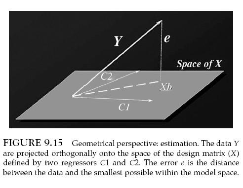
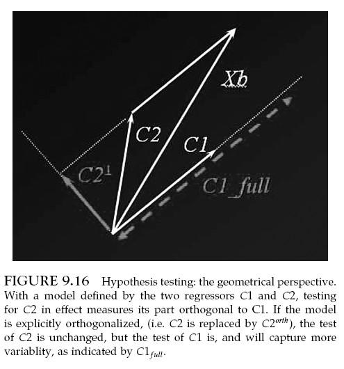
 Elsevier UK Chapter: Ch9-P3756 8-7-6 7:p.m. Page:6 Trim:7.5in 9.5in C H A P T E R 9 Contrasts and Classical Inference J. Poline, F. Kherif, C. Pallier and W. Penny INTRODUCTION The general linear model