Astrophysical Hydrodynamics

Transcription

1 Astrophysical Hydrodynamics i Teacher: Saleem Zaroubi a Room 282, phone 4055, saleem@astro.rug.nl b Office hours: You are always welcome to come to my office for short questions. It is better to set an appointment. ii Teaching assistant: Vibor Jelić a Office: 138, phone: 4050, vjelic@astro.rug.nl iii The purpose of the course is to complete the fluid mechanics background needed on astrophysics. iv Problem sets are mandatory and constitute about 30% of the final grade v Written exam at the end of the term 1

2 Astrophysical Fluid Mechanics Bibliography: I. The lecture notes and handouts are the main source of material, there is no one book on which the material is based. However, there are a number of good books that the student can use to clarify some of the topics or for extra material. II. Optional Books: Astrophysical Flows, J. Pringle and A. King, Cambridge University Press Fluid Mechanics, Landau and Lifshitz, (exceptional book but of somewhat higher level). A first course in fluid dynamics, A. R. Paterson, Cambridge University Press. (Introductory level book). 2

3 Astrophysical Fluid Mechanics Topics I Basic equations of ideal fluids IV.Viscous flows: The Navier-Stokes Equations II Incompressible Fluids V.Similarity solutions III Compressible fluids VI.Turbulence a Waves VII.Magnetohydrodynamics b Hydrodynamics Instabilities VIII. More Astrophysical applications c Shock waves 3

4 I. The basic ideal fluid equations I.1 The Fluid approximation: approximation The fluid is an idealized concept in which the matter is described as a continuous medium with certain macroscopic properties that vary as continuous function of position (e.g., density, pressure, velocity, entropy). That is, one assumes that the scales over which these quantities are defined is much larger than the mean free path of the individual particles that constitute the fluid. 1 lmfp ~ n Where n is the number density of particles in the fluid and s is a typical interaction cross section. Furthermore, for gases the kinetic energy of particles satisfies Ek>>DE, where DE is the energy required to unbind a pair of particles in the medium. 4

5 Solid vs. Fluid A B C D A B A B C D Solid Before application of shear A B C D D C After shear force is removed Shear force A A B B Fluid C D C D 5

6 0. Mathematical preliminaries Gauss's Law Stoke's Theorem 6

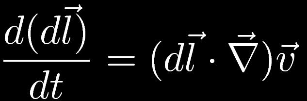
7 Convective (Material, Lagrangian) Derivative Consider the change in a given field, say the density within a volume element moving with the fluid. After time δ t the density within the volume element is. Therefore the change that the density experience is: δt d r v t ;t t r ;t = dt t = v t This derivative is normally called the convictive (Material or Lagrangian) derivative. Notice that if you fix the volume element in space then the equation becomes the normal partial derivative: r, t t r, t t = t Lagrangian vs. Eulerian Description of Fluids: The first involves a coordinate system that moves with the Fluid while 7 the latter involves a coordinate system fixed in space.

8 I.2 The Continuity equation (mass conservation) Consider a volume V which is fixed in space and enclose by a surface where is the outward pointing normal vector. The total mass of the fluid in V is V dv where ρ(r,t) is the density of the fluid. The rate of change in the mass within V is equal to the mass flux into V across it surface. Using the divergence theorem (Green's formula) one obtains Since this holds for every volume this relation is equivalent to n n S V One can also define the mass flux density as which shows that the last equation is actually a continuity equation: 8

9 I.3 Euler's equation (momentum conservation): The Euler (momentum) equation is obtained exactly in the same way the continuity equation is obtained with the following exceptions: 1- The volume we consider is moving with the fluid, i.e., the rate of change is determined by the convictive derivative. 2- The total change in the momentum of volume V is given by the total force working on the particles. This force has many component. The first is the integral of the pressure (force per unit area) over the surface S (at this stage we'll ignore other stress tensor terms that can either be caused by viscosity, electromagnetic stress tensor, etc.): Furthermore, an external force will have to be added as, Where is the force per unit mass, also know as body force. Therefore, the momentum change rate within a volume V satisfies the following integral equation: The left hand term of equation (I.3) is: Where the first equation is to the fact that rdv, i.e., the mass within dv is invariant. 9

10 I.3 Euler's equation (momentum conservation) Applying the divergence theorem to the first right hand term of equation (I.3) yields, Since this is valid for any arbitrary volume, the following differential equation always holds for an inviscid medium. In this discussion we ignored energy dissipation processes which may occur as a result of internal friction within the medium and heat exchange between its parts (conduction). This type of fluids are called ideal fluids. Gravity: 2 =4 G where For gravity the force per unit mass is given by 10

11 I.4 Some thermodynamics Since there is no heat exchange in the flow the entropy per unit mass, s, for any parcel of mass remains constant, namely: Which, together with the continuity equation, yields an entropy density continuity equation: where is the entropy flux density. Notice that this does not imply a constant entropy per unit mass across the fluid, but it means that there is no entropy exchange between different parcels of the flow. However, if the flow started from uniform entropy value the fluid will maintain this value at each point during the flow. A flow with uniform constant entropy is said to be isentropic. Let us define a barotropic flow as a flow in which the pressure is a function of the density only. In such case the enthalpy, H, which is defined as dh=tds+vdp is given only by the second term, i.e., dh=vdp=dp/r. Notice that barotropic flow is more general than isentropic flow. In general the flow could have many other thermodynamic properties, e.g., isothermal, isobaric or isochoric (with constant temperature, pressure or density, respectively) 11

12 I.5 The vorticity equation For barotropic flow (we'll assume that all external forces are conservative, namely drawn from a potential) the Euler equation takes the form Now one can use the relationship Which is derived from the identity: And apply the curl operator to the two side to obtain: Where is called the vorticity 12

13 I.6 Kelvin's circulation theorem For barotropic flow (we'll assume that all external forces are conservative, namely drawn from a potential). Consider the circulation integral, = C v l where the curve C is a closed curve that is moving with the fluid (material curve). Now we the convictive derivative of G, namely we want to explore the change of this integral around a fluid contour as it moves about. Notice, this is not a fixed contour in space. d d v d = l v C dt l dt C dt d = C H f l C v v dt barotropic zero d d S =0 = H f l = H f C S dt Stokes theorem 13

14 I.6 Kelvin's circulation theorem (cont.) For an infinitesimal circulation, one obtains, = C v l S v d S = S d S =constant Namely, the vorticity moves with the fluid. Implications: Imagine that the fluid is getting compressed along the flow lines then Kelvin's theorem implies the the surface are gets smaller, therefore, the vorticity increases. This could be view as conservation of the angular momentum within the material curve. Example: The early Universe went through a phase of very rapid expansion called the Inflationary phase in which the scale of the Universe increased by about 60 e-folds. Therefore, decreases by 120 e folds. As a result any primordial vorticity (so called vector fluctuations) gets completely suppressed 14

15 I.7 Steady flow and Streamlines Steady flow is a flow in which the velocity, density and the other fields do not depend explicitly on time, namely / t=0. Streamlines: A streamline is a line whose tangent is parallel to the fluid velocity at each point in space. A streamline element,, satisfies: In steady flow streamlines do not vary with time and coincide with 15

16 I.8 The Bernoulli equation For barotropic steady flow Euler equation, ignoring external forces, becomes: v 1 v 2 v v = H v H v v v v = v 2 = / l Now the operator, v the last equation becomes the change along a streamline. Therefore, v 2 / 2 H =0 l known as Bernoulli's law and along streamlines could be written as 2 2 v /2 H =v / 2 P / U =constant Under constant gravitational force, g, v 2 /2 H gz =constant 16

17 I.9 Hydrostatics In hydrostatics no flow occurs. This reduces the fluid equations to very simple ones In such a case the fluid equations become: Examples: 1. Archimedes' theorem: A fluid in hydrostatic equilibrium has a uniform density show that is a body is immersed in it, the body experience a force equal to the gravity force exerted on the fluid that the body displaced and opposite in direction. The force that is experienced by the displaced fluid (prior to displacement) by the its surroundings is 17

18 I.10 Hydrostatic equilibrium for a spherically symmetric self gravitating Body The two equations that govern the system are: We'll start from the second equation, the grad and Laplacian operators in spherical coordinates are: Therefore, the hydrostatic and Poisson equations become: 18

19 I.10 Hydrostatic equilibrium for a spherically symmetric self gravitating Body (cont.) Integration of the second equation gives where Now we add the assumption that we have an ideal gas, namely, We also have to decide how µ (the molecular weight) and T behave. Here we'll assume they are constants. A flow that have fixed temperature is called isothermal and c is called the isothermal sound speed. This assumption results in the equation Which has the solution = c 2s 2 Gr 2, p= c 4s 2 Gr 2 This is the well known isothermal sphere solution. Notice that it is singular at the center. Nevertheless it provides a useful analytic approximation for various astronomical problems (sometime with added core). In real stars the temperature and, with it, the pressure increase with depth which provide enough support against self collapse without the need for the singularity at r=0. 19

20 I.11 The Virial Theorem Consider Euler equation of a self gravitating fluid and remember that the velocity vector is given by Hence Euler's equation can take the form: We then multiply both sides of the equation with volume: and integrate over the whole The LHS of this equation could be written as: where are the moment of inertia and the total kinetic energy of the fluid. The first term in the RHS could written as: With the first term is zero due to vanishing pressure at the boundaries. 20

21 I.11 The Virial Theorem (cont.) The last term on the RHS is the one controlled by gravity and could be written as: Where Φ is the total gravitational energy. 21

22 I.11 The Virial Theorem (cont.) Finally we arrive to the relation we are after, which also known as the scalar virial theorem: One can also derive a tensor virial theorem which could be obtained by multplying the ith component of Euler's eq. With the jth component of the radius vector,. This equation take the form: where, 22

23 I.12 The energy and momentum fluxes The Energy Flux: Let us now consider the change of the energy per unit volume in a fluid at a fixed point in space (Eulerian coordinate). The energy per unit volume is composed of two components, the kinetic energy per unit volume and the internal energy per unit volume. The rate of change in the energy per unit volume is,, where U is the internal energy per unit mass. The first component can be shown, using the continuity and Euler's equation, to satisfy the equality, Using the thermodynamic relation one obtains For the ρu part we use the thermodynamic relation which leads (where ). 23

24 I.12 The energy and momentum fluxes (cont.) Therefore, U s v T v s t =H t T t = H Combining these results we obtain t 1 2 v2 U = [ v 2 v 2 H ] 1 The last equation is a continuity equation, where one can identify the term v 12 v2 H as the energy flux term. There is a difference however between what appears in the RHS and the LHS of the equation. In the energy flux the energy that appears is the enthalpy. This has a simple explanation if one writes the integral of the two side over a volume, namely, calculate the rate of change of the energy within a given volume V, the RHS could converted to a surface integral of the following form S v 1 v2 H ds = S v 1 v2 U d S p v d S 2 2 S The first term on the right hand side represent the flux of kinetic and internal energies while the second is the work that is done by the pressure on the fluid in the volume V. 24

25 I.12 The energy and momentum fluxes The Momentum Flux: Similarly the rate of change in the momentum per unit volume is, where the continuity and Euler equations have been used. One could further proceed by defining the tensor which could be placed at the RHS of the previous equation Pik is called the momentum flux density tensor. In the future we'll show that accounting for viscosity in the fluid equations could be easily done by adding another tensor, the viscous stress tensor, to the tensor P. Through integrations over a given volume one can easily see that the RHS of the last equation gives a surface integral over, which is interpreted as the change in the momentum across a surface due to the pressure forces and the actual flow of the momentum through the surface. 25

26 I.13 Boundary conditions The equations of motion have to be supplemented by initial and boundary conditions. The initial conditions normally give the flow properties t the t=0 (but not necessarily). The boundary conditions give the conditions which the fluid has to satisfy at the surface bounding the fluid. For example, if the surface is at rest then the perpendicular component of the velocity at the surface must vanish, i.e., v.n=0. If the surface is moving then the perpendicular velocity at the surface must have the same value as the velocity of the surface. There are other types of boundary conditions that might apply and those will depend on the problem at hand. For example in astronomy boundary conditions could be asymptotic (e.g., density of galaxy drops to zero at infinity) 26

27 I.14 Potential flow Potential floe is a flow in which the vorticity vanishes everywhere in the fluid, i.e.,. In such case Euler's equation could be written as: In such case the velocity could be drawn from a potential, y, or v= y. For barotropic and potential forces, Euler's equation then becomes very simple. or Where f is the force potential and T(t) is some function of time. 27

28 II.1 Incompressible fluids Incompressible fluid is a fluid in which the density within a fluid parcel is constant, namely, dr/dt=0. If this is combined with the continuity equation one obtains that for incompressible fluid, If the flow is also potential then one of the equations of motion become Laplace equation. There are many other properties that one can develop for incompressible fluid, however, we'll develop some of those when we discuss viscous flows. 28

29 I.13 Example of Potential incompressible flow Potential floe is a flow in which the vorticity vanishes everywhere in the fluid, i.e.,. In such case Euler's equation could be written as: In such case the velocity could be drawn from a potential, y, or v= y. For barotropic and potential forces, Euler's equation then becomes very simple. or Where f is the force potential and T(t) is some function of time. 29

30 II.2 Incompressible example A uniformly rotating incompressible fluid (liquid) calculate the shape of the fluid surface given that a uniform and constant gravitational force is acting on it. This problem is a steady flow problem, however if one chooses to view the fluid from a rotating frame of reference the fluid becomes static with the following equations with the solution: At the surface p=p0 which gives the famous parabola solution. If the fluid is not at rest relative to the rotating frame then one has to consider Coriolis forces which normally are much more important that the centrifugal force (e.g., the Earth's weather system). 30

31 III. Compressible flows III.1 Sound waves Consider a small perturbation to a uniform state of a fluid in hydrostatic equilibrium, Then the Fluid equations become: Apply the operator / t on the first equation and on the second: 31

32 III.1 Sounds waves (cont.) In order to solve the system we need another equation. For an ideal fluid with adiabatic fluctuations we can add the equation Which yields 2 1 t 2 p 2 1=0 s This equation could be written as where the adiabatic speed of sound cs is, Homework: do the same thing for isothermal fluctuations 32

33 III.2 Time scales in a fluid The sound speed is a fundamental quantity characterizing a compressible fluid. It sets the maximum speed in which information about pressure, density, velocity and temperature can pass through the fluid. Therefore, if one has a system with a typical scale length, L, pressure, p and density r, then the typical time scale for the fluid to react is: τ L/(p/r)1/2. Now, if the system has other forces like gravity, they come with their own time scale. For example gravity acts within a time scale, known as the dynamical time scale, of τ dyn 1/(Gr)1/2. In gravitational collapse problems the dynamical time scale and the sound speed time scale are present, if the dynamical time scale is much shorter than the hdyrodynamical time scale then the fluid has no time rearrange itself to adjust (i.e., resist) to the collapse and system will collapse until other forces if any overcome Gravity. Whereas if the hydrodynamical time scale is shorter than the dynamical one 33 then the system will adjust in time to equilibrate Gravity (e.g., in stars)

34 III.3 Surface Gravity waves As a second example of small fluctuations we consider incompressible fluid with constant density which occupied a region z < 0 and under the influence of constant and uniform gravitation force This is a reasonable model for ocean waves in deep water. The fluid equations for is: which after taking the divergence becomes We seek a solution of the form: Laplace equation solution is: The condition that perturbation is finite everywhere yields B=0 34

35 III.3 Surface Gravity waves (cont.) Now let us solve for the z component of the velocity: which gives: From this one can obtain the the displacement at the boundary The RHS of the last equation is due to the change in the energy due to the pressure work, while the LHS is due to gravity and these two must be equal. Therefore one obtains the dispersion relation, Therefore, the group velocity of these waves increases with wavelength: 35

36 III.4 Hydrodynamical Instabilities In the previous section we discussed fluctuations that either oscillate to produce wave phenomena or decay. However a third category is also possible, perturbations that grow exponentially rendering the system unstable. A useful way to view the reaction of a system to perturbations is to write the perturbation fields (normally possible to do) in the following form: Obviously the type of reaction the system has to these perturbations. i.e., stable, oscillating or unstable, depends on whether g is negative, zero or positive. respectively. Here we'll deal with a number of instabilities that are common in astrophysical systems. 36

37 III.5 Convective Instability Convection plays an important role in stellar interiors and planetary atmospheres. Here we'll consider a simple stratified fluid under constant gravity force in equilibrium. A small parcel of material is displaced adiabatically while remaining at pressure equilibrium. perturbed position The equilibrium condition The adiabatic condition (p=k rg) The parcel is heavier: stable The parcel is lighter: unstable 37 Initial position

38 III.5 Convective Instability (cont.) Which leads to the instability criterion: Recall that the equation of state for an ideal fluid is given by p=(r/m)rt. In the case of a constant molecular weight (uniform chemical composition) the previous instability criterion becomes: This is known as the Schwarzschild criterion for instability. 38

39 III.6 Rayleigh-Taylor and KelvinHelmholtz Instabilities Rayleigh Taylor Instability The Crab nebula 39

40 III.6 Rayleigh-Taylor and KelvinHelmholtz Instabilities (cont.) Kelvin Helmholtz Instability 40

41 III.6 Rayleigh-Taylor and KelvinHelmholtz Instabilities (cont.) ξ Consider the basic flow of incompressible inviscid fluids (1) and (2) in two horizontal parallel infinite streams of different velocities U1 and U2 and densities ρ1 and ρ2, the faster stream above the other. The two z fluids are immiscible (i.e., do not mix). The force pre unit mass is g^ For both sides. Now suppose that the fluids are perturbed weekly at the surface at which z=ξ the following equations hold: 41

42 III.6 Rayleigh-Taylor and KelvinHelmholtz Instabilities (cont.) The first equation is the perturbation velocity along the z direction: which yields,, where U is the unperturbed fluid velocity. The other equation that the system satisfies is Bernoulli's equation. where B is a constant. We write equation to first order: The constant is Finally we get and expand the last (obtained from the unperturbed case). 42

43 III.6 Rayleigh-Taylor and KelvinHelmholtz Instabilities (cont.) The requirement that the pressure at the surface of discontinuity should be equal yields: We substitute Laplace equation solutions of the form (see disussion on surface gravity waves): Resulting in the following equations at z=0: Requiring a nontrivial solution yields: 43

44 III.6 Rayleigh-Taylor and KelvinHelmholtz Instabilities (cont.) This solution is unstable when the argument of the square root is negative. Which clearly happens when: If U1=U2=0 then the instability is know the Rayleigh Taylor instability while if there is no gravity the instability is known as Kelvin-Helmholz instability. 44

45 III.7 Jeans Instability Assume an infinite homogeneous and self gravitating gas cloud with unperturbed, which are position independent. A side comment, such a setup is unphysical in Newtonian mechanics, still, Jeans ignored this and went ahead with his perturbative approach, this is know as the Jeans swindle. The first order Euler equation gives: Taking the divergence of both sides yields: Suppose now that the gas is ideal and isothermal then the last equation could be written as: where we used the continuity equation as well. ct is the isothermal sound speed. 45

46 III.7 Jeans Instability (cont.) Now we try the usual form of solution to obtain The system is clearly unstable if the dynamical time scale is smaller than the hydrodynamical time scale. Put differently, the instability criterion is: where λj is called the Jeans wavelength. Now if the cloud is roughly spherical one can define Jeans radius (RJ= λj/2). From this one can define a Jean mass, which gives the problem a simple interpretation. If the mass associated with the perturbation exceeds Jeans mass then the system can't react to it in time and the it becomes unstable. 46

47 III.8 Shock waves: supersonic flow Mach number, is the ratio between the fluid ambient speed and the ambient speed of sound, i.e., This could also be interpreted as the ratio between the flow of kinetic energy to the thermal energy through the fluid. Flow with M<1 is called subsonic while that with M>1 is called supersonic. Assume a point is travelling with supersonic speed v speed, the opening angle of shock is given by: 2c t ct vt θ vt 2vt 47

48 III.8 Shock waves (cont.) 1D Shock: This section will develop relations for normal shock waves in fluids with general equations of state. It will be specialized to perfect ideal gases to illustrate the general features of the waves. Assume for this section we have: one dimensional flow. steady flow no area change viscous effects and wall friction do not have time to influence the flow heat conduction and wall heat transfer do not have time to influence the flow. 48

49 III.8 Shock waves (cont.) Since the problem is self similar, one can show that the only solution that satisfies the gas dynamics equations is one in which the fields are constant. Our aim is to describe the disturbance properties (v2,p2,r2). In the lab frame the problem is unsteady, therefore we transform it into another frame in which the problem is steady. 49

50 III.8 Shock waves (cont.) Therefore, we use Galilean transformation to frame that moves with the disturbance assuming that the disturbance speed, D, is known. The idea is then to find the downstream fields (with index 2) and then to invert them in order solve for D. Rankine Hugoniot equations (the shock jump conditions): These equation are basically the conservation laws across the shock which are as follows: [Despite the mathematical issues with deriving these equations in the way we did (a more proper treatment should be employed), these equations are correct. ] 50

51 III.8 Shock waves (cont.) Across the shock these equations yield: Substituting the mass equation in the momentum equation we obtain Which is also known as the Rayleigh line [a line in (p,1/r) space] 51

52 III.8 Shock waves (cont.) Let us manipulate the energy equation to obtain: Substituting from the Rayleigh line one obtains the Hugoniot equation: which is independent of the shock wave speed and the equation of state and indicatesxs that the change in the enthalpy is basically the pressure change times the mean volume. For Ideal gases the relation, holds. Therefore, the Hugoniot equation, after some manipulation, becomes: 52

53 III.8 Shock waves (cont.) 53

54 III.8 Shock waves (cont.) There are two solutions for the intersection between the Rayleigh line and the Hugoniot curve. The first is basically r1=r2 which is not interesting. The second solution gives: with For a strong shock (M>>1) the density ratio is constant For g=5/3 this ratio is 4. While for the acoustic limit (M=1) it is 1. 54

55 III.8 Shock waves (cont.) Back substitute to get For a strong shock (M>>1): Transform back to the lab frame one obtains: Finally yielding: Notice that D always exceeds the speed of sound. 55

56 IV.1 Viscous Fluids One of the main things we neglected so far is to account for internal friction, viscosity, in the fluid. In order to so we have to modify the form of the stress tensor that we have discussed earlier. where the term si,k is called the stress tensor and s'i,k is called the viscous stress tensor. The stress tensor gives the rate of momentum that is not due to direct mass transfer with the moving fluid. In other words the transfer of momentum due to pressure and friction. s'i,k is caused by friction it arises from two adjacent fluid parcel that are moving relative to each other. Therefore it must depend on 56 the velocity gradients across the flow.

57 IV Viscous Fluids (cont.) Assuming no abrupt jumps in the velocity field at infinitesimal distance the momentum transfer must be a linear function of the first derivative of the velocity. Also it can have no constants as the momentum transfer should vanish for uniform flow. There is also no momentum transfer for solid body rotation( ). The most general form the satisfies these conditions is: η and ζ are velocity independent. The first term in the LHS of the equation is traceless and symmetric, whereas the second is diagonal. Notice that for incompressible flow this term considerably simplifies. 57

58 IV Viscous Fluids (cont.) The viscous fluid equation of motion is: η and ζ are called the viscosity coefficients and both are positive. The two are not necessarily constant throughout the fluid. In most fluids the two coefficients do not significantly change. So we'll assume they are constants. The equation of motion then becomes which is known as the Navier-Stokes equation. For an incompressible fluid the 3rd tern in LHS vanishes. 58

59 IV Viscous Fluids (cont.) For vorticity the equation one gets: For incompressible fluid also η is the only viscosity we have to consider. The ratio is called the kinematic viscosity. Here is a table of typical values for η and ν at room temperature. 59

60 IV Viscous Fluids (cont.) Energy dissipation in a viscous fluid: For simplicity we'll assume incompressible fluids and no external forces. We would like to calculate the change of kinetic over the whole fluid volume: We'll choose to to take the time derivative at a fixed volume element is space. Therefore, the time change in the kinetic energy per unit volume is: Which, using the assumption of incompressibility, could be rewritten as: 60

61 IV Viscous Fluids (cont.) Substituting in the integral the first term of the RHS vanishes at infinity (using the divergence theorem). Due to symmetry the second term could be written: Or, Since there is dissipation h has to be positive. 61

62 IV Viscous Fluids (cont.) Two horizontal infinite xz plates with one fixed and the other moving with constant velocity u along the x direction. u h Clearly all quantities are y dependent and the fluid velocity is along the x direction. From the y component of the Navier-Stokes equation we get and from the x component we get. Together with the boundary conditions this leads to 62

63 IV Viscous Fluids (cont.) The force acting on the lower plate per unit area is given by: The only term that counts in this case is which is the force on the lower plate. R Steady incompressible flow in a pipe in the presence of a constant x pressure gradient Since the flow is steady the only relevant velocity component is along the axis of symmetry. We'll call this component v. The velocity will depend only on r. The x component of the Navier-Stokes equation in cylindrical coordinates is: 63

64 IV Viscous Fluids (cont.) Which could be easily solved with: The constants a and b could be obtained from the boundary conditions by v is finite at r=0 and vanishes at r=r. The final solution is then parabolic: Now let us calculate the mass of liquid passing in the pipe per unit time, Q. This result was found empirically by Aagen in Conclusion: Do Not Smoke 64

65 V. Similarity In such a complex set of equations and boundary/initial conditions it is often useful to try to workout some of the basic properties of the system based on dimensionality arguments. For example bodies that have the same shape are geometrically similar. Therefore, they can be obtained from one another by changing the system's linear dimensions. Obviously, one also need to scale the other scale dependent constants in the problem. A simple example of dimensionality argument is the simple ideal pendulum where the only three parameters in the system are g, m and l. The time scale the is relevant therefore is proportional to. For an incompressible fluid for example, one normally has a typical length l [cm], a typical velocity u [cm/s], a typical density, r [g/cm3], and a typical h [cm/gs]. 65

66 V. Similarity From those one can construct a dimensionless number call the Reynolds number: The velocity, pressure, etc. of the fluid at any point could be written as follows: 66

67 V. Similarity Sedov-Taylor Solution for a blast wave: Examples of blast waves include: atmospheric nuclear explosions, supernova explosions. The wave will look self similar as it is in the strong shock limit until it weakens and then the self similar solution is not valid anymore, which will eventually happen when the blast energy is transfered to the material swept up by the wave. It is of obvious importance to be able to calculate how fast and how far the shock front will travel. Let us make an order of magnitude estimate. The r0 be the density of (pre shock) gas and after time t the radius of the shock is R(t). The mass swept up by the blast wave is 67

68 V. Similarity The fluid velocity behind the shock will be roughly the radial velocity of the shock front,, and the kinetic energy swept by the gas is. There will also be internal energy change which is roughly equal to the post shock pressure The last relation is obtained from employing the strong shock jump conditions for the pressure (see shock tube section). Namely, from: and For strong shocks these result is 68

69 V. Similarity The total change in internal energy is of the order of the kinetic energy. Equating either of the two to the total energy gives: with ε of order 1. Which implies that the shock radius at a function of time is: Which should hold from the beginning of the blast until the shock weakens and one can no longer use the strong shock limit to describe the post shock pressure. Homework: Derive the last equation from dimensional analysis. 69

70 V. Similarity For the full solution of this problem we should actually solve the following equations: The first two equations here are the continuity and Euler equations whereas the third holds for adiabatic expansion (P=krg). The solution of this set of equations will depend on the explosion initial conditions. Fortunately, at late times, when most of the mass has been swept up, the fluid evolution is independent of the details of the initial expansion and in fact can be understood analytically as a similarity solution. By this, we mean that the shape of the radial profiles of 70 pressure, density and velocity are independent of time.

71 V. Similarity We'll cast this solution in terms of the dimensionless quantity. Then one can have equations for the twiddled quantities, these equation can be analytically solved (see figure). This self similarity anszatz and the resulting self similar solution for the flow are called the Sedov-Taylor blast-wave solution, since L. I. Sedov and G. I. Taylor independently developed it. 71

72 V. Similarity The solution satisfies the following conditions: 72

73 VI. Turbulence What is turbulence? Fluid dynamicists can certainly recognize it but they have a hard time defining it precisely and even harder time describing it qualitatively. One feature of turbulence is that it is composed of eddies or vortices. Large vortices continually break up into small ones, which in turn break up into even smaller ones, until the effect of fluid viscosity dissipates the kinetic energy of the smallest vortices into heat. 73

74 VI. Turbulence 74

75 VI. Turbulence: Weak Turbulence At a first glance a quantitative description at least in the weak turbulence limit appears straightforward. Fourier decompose the velocity and density fields, the nonlinear terms will introduce coupling between different Fourier modes (normally called wave-wave coupling). Next, solve this system perturbatively. Obviously, this will work only in the weak perturbation limit, or the so called weak turbulence theory. In this theory, one averages over many realizations of a stationary turbulent flow to obtain an average power spectrum of the field as a function of wavenumber (inverse scale). Then if the energy density scales over many octaves of wavelength, scaling argument could be invoked to infer the shape of the spectrum. This type of argument results in the famous Kolmogorov Spectrum for turbulence which is useful and have been experimentally verified in many cases. Note however, that this type of description does not work for strong 75 turbulence, where the turbulence develops.

76 VI. Turbulence: Strong Turbulence Most turbulent flows come under the heading of fully developed or strong turbulence and cannot be well described in this weak turbulence manner. Part of the problem is that the term in the NavierStokes equation is a strong nonlinearity, not a weak coupling between linear modes which has the following properties: Eddies persist for typically no more than one turnover timescale before they are broken up and so do not behave like weakly coupled normal modes. The phases of the modes are NOT random, neither spatially nor temporally. Namely, the flow has well-defined coherent structures like eddies and jets, suggesting some organization. Intermittency the irregular starting and ceasing of turbulence. Strong turbulence is therefore not just a problem in perturbation theory and alternative, semi-quantitative approaches must be devised. 76

77 VI. Turbulence (Kolmogorov spectrum) When a fluid exhibits turbulence over a large volume that is well removed from any boundaries (solid body) then there will be no preferred direction and no substantial gradients in the statistically averaged properties of the turbulent field. The turbulent velocity field will be idealized as made of a set of large eddies, each of which contains a set of smaller eddies and so on. We assume that each eddy is split roughly half of its size after a few turnover times. This could be described as nonlinear velocity correlation terms that transfer energy from large scale eddies to small scale eddies (energy cascade). 77

78 VI. Turbulence (Kolmogorov spectrum) Lets decompose the velocity field into its Fourier components, i.e., where is the velocity in Fourier space. Remember that. We could then define a Reynolds number that is associated with each scale in the flow, For very large scale Reynolds number is very big and energy lose through viscosity, i.e. dissipation, in the Navier-Stkoes equation is negligible. However, small eddies have a small Reynolds number associated with them and therefore dissipation is important. One could therefore say that the scale at which the turbulence is suppressed is when 78

79 VI. Turbulence (Kolmogorov spectrum) For a stationary turbulent field the transfer of kinetic energy from scale to scale is constant, this is the basis for the derivation of Kolmogorov spectrum. We'll derive the Kolmogorov spectrum in a simplistic manner. We define the total energy per unit mass U which could be written as where is energy spectrum as a function of k. Assuming that the energy transfer from scale to scale is constant and we are considering scales with half the wavelength each step in the cascade then the total energy per unit mass is 79

80 VI. Turbulence (Kolmogorov spectrum) Denote the energy per unit mass per unit time that cascades is q. Then one can write. where we used. which yields. Remember that we have also the relation Combining those together we get,.. for the range The limiting wave numbers are set by the largest scale in the turbulence and the scale at which Reynolds number is ~1. 80

81 VII. Magnetohydrodynamics The Basic Equations The interaction of Magnetic fields with (fully or partially) ionized fluids (plasma) play a major role in astrophysical systems. The equations that describe the fluid in this case are the normal fluid equations (with Lorentz force) in conjunction with Maxwell's equations. Gauss' Law Faraday's Law Maxwell's Equations Ampère's Law and Ohm's law: s is the conductivity. 81

82 VII. Magnetohydrodynamics (cont.) Magnetic Pressure Let us consider the magnetic force term in Euler's equation and use Ampère's Law to obtain: Since the pressure in the right hand side of Euler's equation could be written as the negative of the divergence of the stress tensor, it is interesting to ask whether this could also be done for the magnetic terms? The answer to this is yes and the form of the magnetic stress tensor is: It is easy to show that: 82

83 VII. Magnetohydrodynamics (cont.) Magnetic Pressure Therefore one can write the RHS of Euler's equation: Note that T is the magnetic component of the spatial part of the electromagnetic stress energy tensor. Assume for simplicity that the magnetic field is along the z direction, then this tensor could be written as: Which has clearly two parts, an isotropic part which adds to the normal pressure and anisotropic part. In order to characterize relative importance of the two terms it is useful to define the so called the plasma b: 83

84 VII. Magnetohydrodynamics (cont.) The frozen field theorem The time evolution of the magnetic field could be obtained from a combination of Ampère's and Ohm's laws. The RHS of the above equation contain two terms, the first involves the conductivity is a diffusion term, whereas the second, which involves the velocity, is called the convection term. To determine which of the two terms dominates it is useful to define the so called, magnetic Reynolds number, If Rm>>1 then the magnetic field evolves according to, 84

85 VII. Magnetohydrodynamics (cont.) The frozen field theorem There are two different but equivalent statements of the frozen field theorem. Statement 1: The magnetic flux threading any closed curve moving with the fluid is constant. Statement 2: if a line moving with the flow is a magnetic field initially it will remain so indefinitely. Here we'll prove the first statement (the second requires a lengthy proof). The last equation could be written in terms of the vector potential, The convictive derivative of the magnetic flux through a material surface S. 85

86 VII. Magnetohydrodynamics (cont.) The frozen field theorem Z B = S ~ ds ~ B See next page for proof The magnetic flux within a given area form a flux tube that is constant with the flow. Since the tube can be shrunk to infinitesimal area containing basically one magnetic field line, the theorem basically is applicable for any field line. 86

87 VII. Magnetohydrodynamics (cont.) The frozen field theorem Therefore, Then use the following relations with the equation on slide 82 to get the proof: 87

88 VII. Magnetohydrodynamics (cont.) The frozen field theorem Sunspots 88

89 VII. Magnetohydrodynamics (cont.) Diffusion time scales and reconnection 89

90 VII. Magnetohydrodynamics (cont.) Hydromagnetic waves Next we consider the propagation of small perturbations in MHD. For simplicity, the medium is taken to be homogeneous, static and infinitely conducting with initial constant magnetic field which are slightly perturbed, namely, We also assume isentropic flow which gives. 90

91 VII. Magnetohydrodynamics (cont.) Hydromagnetic waves Combining all of these equation together and assuming a solution of the form. After substituting for the pressure from the last equation and eliminating B1 from the equation next to last, one obtains the following set of equations -- expressed in matrix terms. z ~ k Where VA is called the Alfvèn velocity and defined as: θ ~0 B y x In order to get non trivial solution the determinant should be zero. 91

92 VII. Magnetohydrodynamics (cont.) Hydromagnetic waves It is easy to show that the dispersion relation has three roots: These are called the slow magnetosonic mode, the transverse Alfvèn mode and the fast magnetosonic mode respectively. 92