Physics 106b: Lecture 7 25 January, 2018

Transcription

1 Physics 106b: Lecture 7 25 January, 2018 Hamiltonian Chaos: Introduction Integrable Systems We start with systems that do not exhibit chaos, but instead have simple periodic motion (like the SHO) with N degrees of freedom. We discussed the simple (linear) harmonic oscillator (SHO) in Ph106a, Lecture 6. We discussed how to decompose N coupled SHO s into N decoupled normal modes, in Ph106a, Lecture 18. We discussed Action-angle variables, a choice of variables that simplify the discussion of periodic orbits, in Ph106a, Lecture 12; here s a quick review. One degree of freedom First consider a system with one degree of freedom (q, p) governed by the Hamiltonian H(p, q), which can be solved to give periodic motion. An example would be a simple harmonic oscillator, but more generally the frequency of the motion might depend on the amplitude of motion. We seek a time independent canonical transformation (q, p) (θ, I) (c.f. Ph106a Lecture 11) such that the Hamiltonian H is a function of only I H = H(I). (1) Then θ is an ignorable coordinate, and the conjugate momentum I is a constant of the motion I = 0. The angle θ advances at a constant rate giving the frequency, which will in general depend on the action variable θ = H = ω(i). (2) I The action variable I can be evaluated as an integral over the orbit in the (q, p) plane I = 1 p dq (3) 2π (see Hand and Finch 6.5). The canonical transformation can be expressed in terms of a generating function. We choose the type-2 generating function that depends on the new momentum and the old coordinate. Thus we introduce the generating function S(I, q) with the properties (cf. Hand and Finch 6.2 and Table 6.1) new coordinate θ = S I, (4) old momentum p = S q. (5) We want to find S such that the new Hamiltonian is a function just of I. This is given by the Hamilton-Jacobi equation (cf. Hand and Finch pp 222-5) 1 1 In Lecture 12 of Ph106a and in Hand and Finch, the symbol W was used for the generating function (Hamiltonian s Characteristic Function) for a time independent Hamiltonian leading to a constant Hamiltonian. Here I will use the symbol S which is more common in the chaos literature, although we used this symbol before for the case of time dependent generating functions. Also this is a slightly different form of Hamilton-Jacobi theory than discussed there: we are now using the action variables as the constant momenta rather than the separation variables. 1

2 ( ) S H q, q = H(I) = constant (6) where we have evaluated the Hamiltonian using the momentum from Eq. (5). This is a pde in q for S(I, q) for each I and solves the problem. For the simple case of a linear SHO, in scaled coordinates (m = 1, k = 1, ω 0 = 1), the Hamiltonian is H = (1/2)(p 2 + q 2 ), and is equal to the conserved energy. Hamilton s equations give q = H/ p = p and ṗ = H/ q = q. Every point in the 2-dimensional phase space p, q thus has an associated deterministic flow ṗ, q. After choosing an initial condition (a point in phase space), the conserved energy and the subsequent phase space flow (trajectory) is a clockwise circle. In terms of action-angle coordinates, H = ω 0 I; these are like polar coordinates, where I is a constant of motion, proportional to the energy (in scaled units, E = I), and thus to the radius squared of the phase space circle; and ω 0 = dθ/dt = constant (in scaled units, ω 0 = 1) is the rate at which the point on the circle rotates around it with azimuthal angle θ. A real pendulum (the grandfather clock, Hand & Finch 4.2) is non-linear, is damped, and can be driven from oscillation into rotation. The Hamiltonian phase space flow (setting the damping to zero) is shown here: From Two degrees of freedom Two coupled linear SHOs can be decomposed into two uncoupled normal modes (Ph106a Lecture 18 or H&F ch.9). Each normal mode can be written in terms of action-angle variables. The phase space is 2N = 4 dimensional, but specific initial conditions fix the energies in each of the modes, and therefore the action-angle variables (I 1, ω 1, I 2, ω 2 ). There are thus two constants of motion I 1 and I 2, and the phase-spece trajectories lie on a 2N 2 = 2 dimensional sub-manifold: a circle for (I 1, ω 1 ) and a circle for (I 2, ω 2 ). These form a 2-torus in the 4-dimensional phase space. The phase space trajectory winds around that torus: 2

3 From fig2 Figure-1The-orbits-in-an-integrablesystem-with-2degrees-of-freedom-can-be-visualized-as The ratio of orbiting frequencies Ω = ω 2 /ω 1 is called the winding number; it will be important later! Many degrees of freedom For N degrees of freedom a system for which the same action angle procedure works is called integrable. These are very special systems most Hamiltonians will not be integrable. The integrable system will be the starting point for the perturbation theory, and so I will call the Hamiltonian H 0 (p, q) with q and p N-dimensional vectors of the coordinates and conjugate momenta. Integrability implies we can find a canonical transformation (q, p) (θ, I) such that the new Hamiltonian is a function of just I. The angles θ = (θ 1, θ 2,... θ N ) are ignorable, and the action variables I = (I 1, I 2,... I N ) are constants of the motion. Thus a necessary condition for a system with N degrees of freedom to be integrable is that there are N constants of the motion. This is not sufficient the constants must also be in involution. (This is analogous to the idea of commuting operators in quantum mechanics, that are then simultaneously diagonalizable.) The canonical transformation is given by the generating function S 0 (I, q) with the Hamilton- Jacobi equation for S 0 ( ) S0 H 0 q, q = H 0 (I) independent of θ. (7) The θ j evolve at constant rates ω 0,j with ω 0 = H 0 I or in component form ω 0,j = H 0 I j. (8) The motion is on the product of N limit cycles, i.e. motion on an N-torus. This is of dimension N, compared with 2N 1 for the constant energy surface, so that the integrable dynamics sample a tiny fraction of the constant energy surface. We assume that this part of the problem is solved (e.g. for N balls and springs). The approach to chaos - Preliminaries Hamiltonian dynamics of a single degree of freedom with a time independent Hamiltonian (no energy dissipation) cannot give chaos, since trajectories cannot cross and this restricts the possible dynamics on the two dimensional phase space. The simplest examples of Hamiltonian chaos are 2 degrees of freedom (two positions, two conjugate momenta) with a time independent Hamiltonian. The constraint of constant energy confines the dynamics to a three dimensional surface in the four dimensional phase space. 1 degree of freedom (one position, one conjugate momentum) with a time-varying but periodic Hamiltonian (eg, a regular kick). We first discuss two examples, and then a perturbation approach to the question of when simple periodic motion breaks down to more complex dynamics. We will talk more about the complex dynamics in the next lecture. 3

4 Double pendulum Hand and Finch 11.1 look at this example of the first type, and we also demonstrated it and discussed it in class. For small oscillations, the phase-space trajectory winds around a 2-torus, as discussed above. If the winding number is rational (Ω = r/s, where both r and s are integers), then the trajectory makes r full orbits in ω 2 for s full orbits in ω 1, and then returns exactly to its initial starting point; it is perfectly periodic. You can plot θ 1 vs θ 2 and get a pretty Lissajous pattern. If the winding number is close (in a sense to be described later) to rational, the trajectory will return almost to its starting point; maybe a bit advanced, or retarded, in θ 1 or (equivalently) θ 2. After one more iteration around the torus, it will be displaced a bit more in the same direction. After enough trips around the torus, the trajectory might completely cover the torus. If the winding number is very irrational, it s hard to visualize the 4-dimensional phase space trajectory on the 2-torus. The Poincaré Section Poincaré s idea to visualize this motion was to take a slice (or section ) of the 4-dimensional space; so we only plot, say, I 1, ω 1 (or equivalently, θ 1, θ 1 = ω 1 ), and only when θ 2 passes through zero in the positive direction (one full oscillation or rotation of that degree of freedom). The 2-torus becomes a circle (or ellipse). If Ω = r/s is rational, there will be s distinct points, which will wind around the center of the circle r times. By counting these, you can determine the winding number Ω. If Ω is not rational, the points will fill up the circumference of the circle. The Poincaré section will be our most powerful tool for visualizing the motion of low-dimensional systems that can exhibit chaotic motion. The linear double pendulum motion, confined to the 2- torus, can t become chaotic (although, for irrational winding numbers, it can fill the torus and never return to its starting point; but it s still predictable, and small changes in the initial conditions lead to small changes in the subsequent trajectory). The nonlinear double pendulum We consider an undamped, undriven double pendulum (with, for simplicity, m 1 = m 2 = 1, l 1 = l 2 = 1, g = 1). The system is conservative (total energy is conserved, no dissipation). If the system starts out with small angular displacements (linear regime) near one of the two normal modes, The Poincaré Section shows a fixed point. A small deviation of the initial conditions away from this fixed point evolves into a circle, which is a slice of the 2-torus. If the non-linearity (as determined from the initial conditions, which specify the total energy and the initial point in 4-dimensional phase space) is not too big, the resulting trajectory remains on the 2-torus, but the 2-torus is distorted. The further away one goes from the fixed point, the further into the non-linear regime. The torus slice gets distorted, but still, the trajectory remains on it. We can say that, for these small displacements, the tori are quasi-invariant; it s possible that if we wait long enough, the non-linearity will cause the trajectory to diverge from the torus. 4

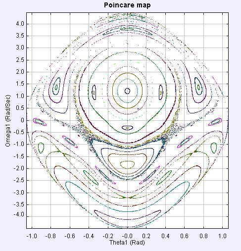
5 Left: The double pendulum near the Mode 1 initial condition. Middle: The phase space trajectory of pendulum bob 1 (θ 1 vs θ 1 = ω 1 ) in Mode 1. Right: The Poincaré section for small non-linearity. Each contour corresponds to the trajectory for one particular initial condition. The red fixed point at (0,0.5) is for Mode 1, and the green fixed point at (0, -1.15) is for Mode 2. Other in-between initial conditions give contours of varying size and distortion, but the trajectories remain on the tori; they remain roughly invariant. From When the angular displacements of the two coupled pendula θ 1, θ 2 are sufficiently large so that the linear approximation sin θ θ is no longer valid, the system can no longer be cast into actionangle coordinates; the motion is no longer solvable analytically; it is no longer integrable. The motion must be followed through numerical integration (simulation), and visualized with the twodimensional Poincaré section: we plot a point in θ 1 vs θ 1 thenever θ 2 passes through zero in the positive direction. When the non-linearity (eg, the total energy) is further increased, the tori begin to break up; chains of 2, 3, or more smaller tori appear. And, in some regions (growing ever larger as the energy is increased) there is simply a chaotic spray of points. If one follows the trajectory through these points, it is increasingly difficult to predict where it will land in the next iteration; even a tiny displacement from such a point will land the trajectory in a completely different region of the phase space slice. This is chaos. Poincaré sections for the higher energy cases are shown on the next page. You are strongly encouraged to download and play with this simulation yourself! (You will need at least version 1.5 of Java (JRE).) 5

6 Appendix 5 Joules. 8 Joules. 10 Joules. 25 Joules. 6

7 Periodically Kicked Rotor This is a very simple example of the second type. K (t-n) Consider a rigid pendulum but with no gravity. The dynamics is given by the angle θ and the conjugate momentum p = θ (taking the moment of inertia to be 1). The pendulum is given a periodic impulsive vertical kick of strength K with period 1 (i.e. a kick at times t = n with n an integer). The dynamics can be reduced to the discrete map for θ n, p n which are the angle and momentum just after the nth kick. At each kick the (angular) momentum changes by the impulsive moment, but the angle doesn t change. Between kicks the momentum is constant and angle increases at the constant rate θ = p. This gives the equations The equations are usually transformed by introducing to give the standard map p n+1 p n = K sin θ n+1, (9) θ n+1 θ n = p n. (10) x n = θ n mod 1, 2π (11) y n = p n, (12) x n+1 = x n + y n mod 1, 2π (13) y n+1 = y n + K sin(2πx n+1 ). (14) Liouville s theorems tells us the map is area preserving the key property of the map linked to the Hamiltonian nature of the dynamics 2. This also follows from direct calculation of the Jacobean ] J = det [ xn+1 x n x n+1 y n y n+1 y n+1 x n y n = 1 (15) 2 The two dimensional map given by the β, l β Poincaré section of the double pendulum considered by Hand and Finch is also area preserving, but this no longer can be deduced simply from Liouville s thoerem. Instead the symplectic property of Hamiltonian dynamics must be used. This is discussed in the appendix to Chapter 6 of Hand and Finch. Actually the form they discuss is not sufficient to prove the map is area conserving because the Poincaré section is not a fixed time slice. Instead the Poincaré-Cartan invariant (p dq Hdt) must be used. This reduces to p dq for a time independent H even when the integral is taken around a loop on the Poincaré section see Hand and Finch for the rest of the discussion. 7

8 Dynamics of the Standard Map For K = 0 (no drive) the system is integrable the rotor rotates at a constant rate determined by the initial conditions. In the iterated standard map this translates into a series of points at fixed y. The appearance after many iterations depends on the winding number Ω which is defined as the average (here constant) advance in x per iteration (or the ratio of the average rotor frequency to the frequency of the periodic kicks). For a rational winding number Ω = p/q, with p, q integers, we see a discrete set of p points. For irrational winding numbers (cannot be expressed in this form) the points will eventually fill in the line 0 x 1. The winding number for K = 0 is just the value of y, so that almost all 3 initial conditions will give an irrational winding number. Even for rational y = y r giving rational winding numbers the line 0 x 1, y = y r is invariant under the dynamics (any point on the line is mapped into another point on the line.) Since x is a periodic variable the lines correspond to closed circles, or one dimensional tori. These are analogous to the circles in phase space describing the normal modes of simple harmonic oscillators and other integrable systems. The study of Hamiltonian chaos begins by seeing how these tori break down on adding the periodic kicks. See the numerical demonstrations to illustrate the result that tori with irrational winding numbers survive adding small kicks, whereas those with rational winding numbers break down to a set of elliptical and hyperbolic fixed points, with chaotic motion in regions surrounding the hyperbolic fixed points. The break down occurs because the rotor motion is resonant with the drive for rational winding numbers. Since the system is periodically driven, an interesting question is whether the kinetic energy (p 2 /2 y 2 ) of the rotor continuously grows. Because the map is area preserving, the initial tori spanning the whole range of x act as barriers to the growth of energy. Thus the break down of the last surviving of these tori is an important event. It happens at K = 1 for the standard map. For larger values of K the energy can increase to large values. It does so diffusively (i.e. the mean over a long time t remains zero, but the variance grows as t. This is known as Arnold diffusion. 3 Almost all is used as a precise term to mean all except a set of measure zero. 8