TIME REVERSAL COMPRESSIVE SENSING MIMO RADAR SYSTEMS NICK SAJADI

Transcription

1 TIME REVERSAL COMPRESSIVE SENSING MIMO RADAR SYSTEMS NICK SAJADI A DISSERTATION SUBMITTED TO THE FACULTY OF GRADUATE STUDIES IN PARTIAL FULFILMENT OF THE REQUIREMENTS FOR THE DEGREE OF DOCTOR OF PHILOSOPHY GRADUATE PROGRAM IN ELECTRICAL ENGINEERING AND COMPUTER SCIENCE YORK UNIVERSITY TORONTO, ONTARIO DECEMBER 2016 c NICK SAJADI 2016

2 Abstract Active radar systems transmit a probing signal and use the return backscatters received from the channel to determine properties of the channel. After detecting the presence of targets, the localization of targets is achieved by estimating relevant target parameters, including the range, Doppler s frequency, and azimuth associated with the targets. A major source of error in parameter estimation is the presence of clutter (undesired targets) that also reflects the probing signal back to the radar. To eliminate the fading effect introduced by backscatters originating from the clutter, the multiple input multiple output (MIMO) radar transmits a set of simultaneous uncorrelated probing signals from the transmit elements comprising the transmit array. A major problem with MIMO radars is the large amount of data generated when the recorded backscatters are discretized at the Nyquist sampling rate. This in turn necessitates the need of expensive, high speed analog-to-digital converter circuits. Compressive sensing (CS) has emerged as a new sampling paradigm for reconstructii

3 ing sparse signals with relatively few observations and at a lower computational cost compared to other sparsity promoting approaching. Although compressive beamforming has the potential of high resolution estimates, the approach has several limitations arising mainly due to the difficulty in achieving complete incoherency and sparsity in the CS dictionary. This PhD thesis will apply the principle of time reversal (TR) to MIMO radars to improve the incoherency and sparsity of the compressive beamforming dictionary. The resulting CS TR MIMO radar is analytically studied and assessed for performance gains as compared to the conventional MIMO systems. iii

4 This thesis is dedicated to my beautiful wife Razieh Niazi, who always supported and encouraged me and two lovely and beautiful daughters Elaheh and Ava who are always my angels. iv

5 Table of Contents Abstract ii Table of Contents v List of Tables x List of Figures xi 1 Introduction 1 2 Estimation in SISO, SIMO, and MIMO Radar Systems SISO Target Parameter Estimation The matched filter - Joint Estimation of Doppler-Range Pulse-Doppler Radar - Joint Estimation of Doppler-Range SIMO Target Parameter Estimation Estimation of the Direction of Arrival (DOA) Estimating DOA using a beamforming algorithm v

6 2.2.3 Joint Estimation of Azimuth and Elevation Uniform Rectangular Time Reversal Arrays: Joint Azimuth and Elevation Estimation Introduction System Formulation Time Reversal Estimating Azimuth and Elevation Cramér-Rao Lower Bounds Simulations and Results Summary Estimation in MIMO Radar Systems MIMO Radar with Collocated Antennas Time Reversal MIMO Radar Systems Compressive Radar Parameter Estimation Fundamentals of Compressive Sensing Sparsity Incoherence Sampling Sparse signal recovery for a noise free sensed signal vi

7 3.1.4 Sparse signal recovery in the presence of additive observation noise Compressive Sensing Single Input Single Output Radar Systems Formulation for the CS/SISO radar system The upper bound in the sparsity of CS/SISO approach Resolution limits Compressive Sensing Multiple Input Multiple Output Radar Systems for Clutter Free Channels System formulation Compressive sensing for MIMO radar Resolution limits Compressive Sensing Time Reversal Radar Systems Compressive sensing for MIMO radar system MIMO system formulation in multipath channels The compressive sensing for the multiple input multiple output (CS/MIMO) radar The compressive sensing for time reversal MIMO radar system TR MIMO Formulation in Multipath radar vii

8 4.2.2 The compressive sensing time reversal multiple input multiple output (CSTR/MIMO) radar Complexity analysis Numerical simulations Performance Bounds for the CSTR/SIMO and CSTR/MIMO Radar Systems Compressive sensing limitation measures The coherence analysis of the CS/SIMO and CSTR/SIMO radar systems The CS/SIMO sensing matrix The CSTR/SIMO sensing matrix Coherency analysis for the CS/SIMO and the CSTR/SIMO sensing matrices CS/SIMO Radar CSTR/SIMO Radar Numerical simulations for the CS/SIMO and the CSTR/SIMO sensing matrices The coherence analysis of the CS/MIMO and CSTR/MIMO radar systems viii

9 5.3.1 Coherence in the CS/MIMO sensing matrix Coherence in the CSTR/MIMO sensing matrix Numerical simulations for the CS/MIMO and the CSTR/MIMO sensing matrices Conclusion and Future Work 167 A Unsupervised Time Reversal based Microwave Imaging for Breast Cancer Detection 171 A.1 Introduction A.2 The Data Adaptive Filter Algorithm A.3 The DAF/EDF Algorithm A.4 Simulations and Results A.5 Summary B List of symbols used in the thesis 191 Bibliography 194 ix

10 List of Tables 1.1 Symbols used for the radar equation The Joint range and Doppler frequency estimation based on the ambiguity function The Capon DOA estimation algorithm Parameters in the simulation shown in Fig The MIMO/CBA plus LSA to estimate the DOA and RCS Symbols used for the forward probing derivation Parameters used in the Monte Carlo simulations Parameters used in the simulations for Figs. 5.1 and Parameters used in the simulations for Figs x

11 List of Figures 1.1 Block diagram of a typical radar A matched filter implementation for estimating range τ 0 and the Doppler shift f d associated with the target using predetermined bins for range τ (i) 0 and the Doppler shift f (j) d. The output of the matched filter contains f(t) delayed by τ (k) 0 = τ 0 τ (i) 0 and frequency shifted by f (l) d = f d f (j) d (a) Mesh plot for the ambiguity function and (b) the corresponding contour plot for a single rectangular pulse (a) Zero Doppler shift cut along the Doppler frequency axis representing the range ambiguity function (b) Zero delay cut along the delay axis representing the Doppler shift ambiguity for a rectangular pulse with W = 4 seconds A coherent pulse train f(t) with N p pulses of duration T (a) Mesh plot for the AF output. (b) Corresponding contour plot for a train of rectangular pulses with W = 0.2 s, N p = 5 pulse/s, and T = 1 s xi

12 2.6 (a) Zero Doppler shift in one dimension obtained from Fig. 2.5 by taking a splice along the Doppler frequency axis representing the range ambiguity function. (b) Zero delay in one dimension obtained from Fig. 2.5 by taking a splice along the delay axis representing the Doppler shift ambiguity function for a train of rectangular pulses with W = 0.2 s, N p = 5 pulse/s, and T = 1 s Delay propagation ras a function of the direction of arrival (DOA) in a uniform linear array (ULA) The Capon array power output P (θ) for a simulation with parameters defined in Table An URA used for joint azimuth φ and elevation θ estimation angles Estimated azimuth and elevation using: (a) TR Capon, and; (b) Conventional Capon for a 2D URA system with one target at a SNR of 10dB RMSE plots and corresponding CRLBs for: (a) Azimuth, and; (b) Elevation obtained from the conventional and TR URA systems (a) A MIMO radar system N t collocated transmit elements and N r collocated receive elements. (b) A MIMO radar system with widely separated transmit and receive elements A MIMO radar system with collocated antennas probing a highly cluttered channel xii

13 4.1 Comparison between the CS/MIMO and CSTR/MIMO radars: (a)-(c) RMSE plots for the DOD (subplot (a)), DOA (subplot (b)), and Doppler shift (subplot (c)). The CSTR/MIMO outperforms CS/MIMO radar for the DOD, DOA, and Doppler shift estimations Error distribution comparison between the CS/MIMO and CSTR/MIMO radars at 5dB SNR: (a)-(c) for the DOD (subplot (a)), DOA (subplot (b)), and Doppler shift (subplot (c)). The CS/MIMO error spreads are wider in the DOD, DOA, and Doppler shift estimates Normalized Gram matrices for the: (a) CS/SIMO radar; (b) CSTR/SIMO radar with N r = 16. Suplots (c) and (d) are the same as (a) and (b), respectively, except for N r = Comparison of the mutual coherence for CSTR/SIMO systems for different array setups Comparing G (CS/MIMO) and G (CSTR/MIMO) using 2D plots for Case I Comparing G (CS/MIMO) and G (CSTR/MIMO) using 3D plots for Case I Comparing G (CS/MIMO) and G (CSTR/MIMO) using 2D plots for Case II with 80% compression ratio Comparing G (CS/MIMO) and G (CSTR/MIMO) in 3D plots for Case II with 80% compression ratio Comparing G (CS/MIMO) and G (CSTR/MIMO) for the ULA setup xiii

14 5.8 Comparing G (CS/MIMO) and G (CSTR/MIMO) for the WR/RLA setup Comparing G (CS/MIMO) and G (CSTR/MIMO) for the NR/RLA setup A.1 The EM breast model derived from the MRI of a patient with the proposed antenna geometry (Arrays A and B) parallel to the chest walls. Normally, the antenna arrays are placed well above the breast with the arrays parallel to the chest wall A.2 The DAF/EDF algorithm A.3 The output of the low pass filter on the mixed response to determine n 0 and m parameters A.4 Estimated target response obtained from the DAF/EDF approach for tumour in the middle of the breast tissue A.5 A spherical 2mm cancerous tumour is introduced at eleven different locations marked as 1 to 11 in the figure A.6 Array imaging pseudospectrum for location 1 and SNR = 30dB obtained from 2 TR array imaging algorithms when tumour response obtained by DAF/EDF algorithm. The tumour location is represented by, while the estimated location is given by A.7 Range of absolute errors (mean ± standard deviation) in estimating the location tumour derived by running a Monte-Carlo simulation at location 1 for the four array imaging algorithms for a SNR of 30dB xiv

15 A.8 Same as Fig. A.7 except for a SNR of 15 db xv

16 1 Introduction Originated before World War II, RAdio Detection And Ranging (radar) is used for detection and and tracking targets. Two types of radar systems are common: active and passive radars. The active radar system illuminates the medium by transmitting a probing signal into the medium, usually called the channel, being investigated. The passive radar system, on the other hand, observes the signal received from active targets and use it for detection. Regardless of their nature, all radar systems are equipped with at least one receiver for capturing backscatters of the probing signal in the case of the active radars. For the passive radar system, the receiver records the signal emitted from targets embedded in the channel. As an example of an active radar system, the airport surveillance radar (ASR) is used to monitor approaching and departing airplanes by consistently transmitting a probing signal and recording backscatters from the airplanes in the proximity of an airport. Astronomers, on the hand, use radio telescopes configured as passive radar systems to capture energy emitted from celestial objects in the cosmos. For an active radar 1

17 Parameter P t G t A r λ G r σ F Definition Transmitter power Gain of the transmitting antenna Effective aperture (area) of the receive antenna Wavelength of t he transmitted signal Gain of the receive antenna Scattering coefficient of the target that is related to the radio/radar cross section (RCS) Pattern propagation factor (PPF), that accounts for the situation when the free space conditions are not met. The PPF is different for the wave propagation path to and from targets. In a vacuum without interference F = 1. R t R r Distance from the transmitter to the target Distance from the target to the receiver Table 1.1: Symbols used for the radar equation. system, the power received by receiver is described by the radar equation, [1], P r = P tg t A r σf 4. (1.1) (4π) 2 Rt 2 Rr 2 with the notation used is defined in Table 1.1. The received power is often represented as a summation of returns (backscatters) reflected from targets and clutters. In the design of radars, the goal is to maximize the power of backscatters reflected from the target, while eliminating unwanted backscatter reflections of the probing signal from clutters. Sources of backscatters are reflection from ground, sea, rain, bird, buildings, and chaff. For example, the ground backscatters may have a power of 50 to 60 db greater than direct reflections from the targets [1]. Because most 2

18 Transmitter Propagation Medium Power Amplifier Waveform Generation Target Radar Cross Section Antenna T / R Switch Signal Processor Computer Receiver A / D Converter Pulse Compression Clutter Rejection (Doppler Filtering) General Purpose Computer User Displays and Radar Control Data Recoding Tracking Parameter Estimation Thresholding Detection Figure 1.1: Block diagram of a typical radar. clutters are relatively stationary as compared to targets, the Doppler shifts associated with clutter backscatters are relatively small. Using the clutter Doppler shift, clutter backscatters may potentially be removed by filtering the received power for the low Doppler shift backscatters. After analog to digital conversion (ADC) and removing the clutter effect from received backscatters, there are three main steps taken in any radar system: (a) Detecting the presence and absence of targets; (b) Estimating the parameter associated with the targets and; (c) Tracking the target (Fig. 1.1). The outcome of the detection process is to verify the presence of the 3

19 target in the channel under investigation. The estimation process determines the parameters (range, velocity, and direction) associated with the target while the tracking process tries to minimize the error associated with the estimation process. In this document, we focus on the estimation process for radar systems. We are interested in estimating the target parameters used for target localization including range, velocity, and directional angle. Note that, not all parameters can be estimated by all radar types. For example, a stationary single input single output (SISO) radar is able to estimate the range and velocity of the target. A rotatory SISO radar is able to detect the angle by reducing the range and use of a sophisticated beam pattern. For estimating the angle in a stationary long range radar, the single input multiple output (SIMO) or the multiple input multiple output (MIMO) setup is required. (1) Range: The emitted energy from the transmitter to scatters (targets and clutters) and from scatters back to the receiver has a flight time based on the wave propagation speed c. The flight time is captured as a round-trip time delay τ 0 representing the range of each scatterer. Once the round-trip time delay τ 0 is estimated, the range is estimated simply by using c τ 0 2. Because of the simple and tight relationship between the range and time delay, the two terms are used interchangeably in this document. Conventionally, the time delay τ 0 in radar systems is estimated using the matched filter. The resolution (resolving two or more scatterers 4

20 from each other) of the matched filter depends on the shape of the a well as inter probing delay time. (2) Velocity: While clutters are mostly stationary, targets are usually dynamic. The motion of a target shifts the frequency contents of probing signal. An approaching targets shifts the signal toward higher frequencies. A bandwidth shift toward a lower frequency represents a target moving away from the radar platform. The shift in the bandwidth of the probing signal is referred to as the Doppler shift. The sign and magnitude of the Doppler shift corresponds to the target velocity vector. For a narrowband probing signal, the frequency shift (Doppler shift) of the carrier frequency f c = c λ c is given by 2vt λ c for a target moving toward a stationary receiver with velocity v. For a slow moving target, i.e., 2v λ c 1 W with W the probing signal time width, the Doppler shift is insignificant. Conventionally radar systems use a two dimensional matched filter for jointly estimating the range and Doppler shift. The resolution quality of the matched filter is often studied using the ambiguity function. To improve the resolution of the matched filter for the Doppler shift, several pulses are transmitted with the pulse repetition interval (PRI) T during the transmitting stage. (3) Angle: Target localization without estimating the angle is incomplete. Given the range of a target is known, the location of the target can be anywhere on the surface of a hemisphere with a radius equal to the range of the target. To esti- 5

21 mate the angle of the received power P r for a scatterer, radar systems are equipped with more than one receiver. Assuming an array, the interelement (inter receiver) spacing generates a spatial delay corresponding to the angle θ and the distance of each receiver to the radar platform reference element. To estimate the target angle θ, the output of all receivers are processed with spacial algorithms known as beamformers. Beamformer algorithms typically use a matrix known as steering matrix or calibration matrix for the array setup. To estimate the directional angle associated with the target the output of receiver elements are correlated. The estimated target angle θ corresponds to either the azimuth or elevation angle. To estimate both azimuth and elevation angles simultaneously, the receiver elements are scattered over a plane. The corresponding steering matrix is formed for both the azimuth and elevation angles such that the beamformer algorithm is able to estimate both angles simultaneously. The clutter rejection process in the radar block diagram is depicted in Fig It removes static clutters with low Doppler shifts from received backscatters. However, when targets are close to clutters, they have the same Doppler shifts due to the secondary reflections between targets and clutters. In a cluttered channel where targets are close to clutters (as is the case for a low altitude airplane), secondary reflections between targets and clutters cause a fading effect on target backscatters. Fading is undesired because it degrades both target detection and estimation pro- 6

22 cesses [2,3]. One way to cope with the fading effect is to use multiple input multiple output (MIMO) radar systems [2, 4]. In the MIMO radar system, several transmitters probe the channel simultaneously with uncorrelated probing signals. Because of uncorrelated probing signals, the fading effect diminishes in the MIMO radar systems. In a highly cluttered channel with close proximity between targets and clutters, however even the detection and estimation performances of MIMO radar systems are degraded. To improve the performance of radar systems in a highly cluttered channel, the time reversal (TR) radar is coupled with the MIMO radar. In the TR radar, the channel under investigation is probed a second time with the normalized and time reversed version of the signal received in the first transmission. While the second probing stage, known as TR probing stage, highlights the backscatters from targets, clutter backscatters due to the secondary reflections are diminished. The highlighting target backscatters and diminishing clutter backscatters effect is known as the TR superresolution focusing [5, 6], which has proven to enhance the radar detection and estimation processes [7, 8]. In order to apply the clutter rejection, detection, and parameter estimation processes in radar systems, the analog to digital converter (ADC) unit should at least sample received backscatters at the Nyquist sampling rate of twice the highest frequency present in the received backscatters. The ADC unit consumes a high amount of energy to produce samples at the Nyquist rate. Sampling at the Nyquist 7

23 rate produces a large amount of data which in turns needs a huge amount of space and energy to record data. If the ADC samples less than the Nyquist rate, the sampled received backscatters has aliases which degrades the performance of all radar processes dramatically. Recently, the compressive sampling (CS) approach has been introduced to sample the backscatters recorded at the receive elements at rates much below the Nyquist sampling rate under the coherence and sparsity conditions [9 11]. The coherence is related to a space which models under sampled received backscatters known as compressed received backscatters. The space is usually represented as a matrix known as the sensing matrix Θ and coherence is referred to the maximum correlation of columns of the sensing matrix Θ. If the number of scatterers in the channel are considerably less than the columns of the sensing matrix, the received backscatters may be modeled as a sparse signal. Given such a sparse signal, the original received backscatters can be recovered by applying a convex minimization algorithm [9 12]. Lower the coherence, higher is the probability that the CS approach will recover the original sparse signal with accuracy [11, 12]. While the CS approach was originally introduced allow for signal reconstruction from it samples obtained at rate lower than the Nyquist rate, the CS approach may alternatively be extended for target parameter estimation if the signals are sampled at the Nyquist rate [13 22]. For the target parameter estimation, the sensing 8

24 matrix columns represent different possible values of target parameters. Given the coherence of the sensing matrix Θ and sparsity of received backscatters, one can sample received backscatters at much less than the Nyquist sampling rate and estimate target parameters from compressed received backscatters using a convex minimization algorithm. The output of the convex minimization algorithm is a vector in which nonzero elements determines the target parameters corresponding to columns of the sensing matrix Θ. Although the applicability of the CS approach for estimating target parameters is shown in References [13 22], the coherence and sparsity conditions can be easily violated especially for a highly cluttered channel. As a result, the applicability of the formulated CS approach for radar applications is limited for real life scenarios with clutter. Based on the time reversal (TR) superresolution focusing, we propose coupling time reversal with compressive sensing to satisfy both incoherence and sparsity conditions. The coupling of TR and CS approaches provides higher chance of applicability of the CS approach to real life scenarios for target parameter estimation. The contributions of my thesis are summarized as follows. Contributions 1. Application of Time Reversal to 2D arrays: As a first contribution of the thesis, I propose a time reversal based uniform rectangular array (TR/URA) 9

25 system for joint estimation of azimuth and elevation of a stationary target. I derived closed-form, analytical expressions for Cramer Rao lower bounds (CRLB) for both conventional and TR/URA systems configured as two dimensional (2D) arrays and performed Monte Carlo simulations to illustrate the superior performance of the TR/URA system over its counterparts without TR. Since the thesis is primarily focused on one dimensional, linear arrays, these results are included in Appendix 2.3 to maintain the flow of the thesis. This work has appeared previously in [23]. 2. Compressive Sensing Time Reversal Radar: The thesis applies compressive sensing (CS) and time reversal (TR) to linear arrays. A novel algorithm for joint estimation of the direction of arrival, direction of departure, and Doppler information is derived on potential targets embedded in an environment with rich clutter. The CSTR radar uses multipath constructively and offers significant performance gains over its CS counterpart without TR in our Monte Carlo simulations. To the best of my knowledge, this is the first application of CS to time reversal MIMO radars. This work was published partly in [24]. 3. Extension of CSTR theory to MIMO radars: The CSTR algorithm listed under item 2 is extended to MIMO radars. The CSTR/MIMO radar is not a straightforward extension of the single-input, multiple-output (SIMO) system 10

26 since the final observation recorded in TR has a correlated noise component. Using the results in [25], which shows that the noise component in the TR observation can be modelled as white noise, we derive joint estimation algorithms for direction of arrival, direction of departure, and Doppler information for the CSTR/MIMO system. Time reversal converges the TR probing signal on the target leading to a stronger backscatter from the target as compared to the ones received from surrounding clutter. This super-resolution focusing results in significant improvement in the estimation performance of the CSTR/MIMO radar. Monte Carlo simulations verify the superiority of the CSTR/MIMO radar over its CS/MIMO version without TR. Selected sections of this work has appeared in [26]. 4. Performance Analysis of SIMO Compressive Sensing Time Reversal Radars: To verify the improvement offered by the CSTR/SIMO systems, an analytical expression for the mutual coherence of the CS dictionary is derived. In compressive sensing literature, incoherency is often used as a defining parameter for verifying potential gains with CS. In this thesis, I have verified the increase in the incoherency of the CS dictionary with time reversal in CSTR/SIMO systems versus CS/SIMO systems both analytically and through Monte Carlo simulations. This work has appeared recently in [27]. 11

27 5. Extension to MIMO Compressive Sensing Time Reversal Radars: In addition the coherency comparison for the CS/SIMO systems with and without TR, coherency analysis is completed for both CS/MIMO and CSTR/MIMO radars in the second half of Section 6. Through analytical derivations, I show that dictionary for the CSTR/MIMO radars is more incoherent than the corresponding dictionary for the CS/MIMO systems that results in CSTR/MIMO radar outperforming CS/MIMO radar without TR. Monte Carlo simulations corroborate the results obtained from the analytical derivations. 6. Application of TR Array Processing in Breast Cancer Detection: As an exploratory application of TR to magnetic resonance imaging (MRI), Reference [28] derives an algorithm for breast cancer detection based on TR. To remove the effects of clutter (skin, bones, and rip cage in the case of humans), I use the background subtraction step in [28] that eliminates the reflections arising from the clutter. Recall that background subtraction makes an additional measurement of the medium in the absence of the target and subtracts the recorded data from the actual observation when the target is present. In military applications, the background subtraction step is fairly common. It can not be utilized in medical applications since access to a tumour-free medium for a sick patient is not available. In [29], I proposed a new clutter suppression algorithm that successfully isolates the tumour response from the 12

28 overall (tumour and clutter) response. The proposed approach is based on a combination of the data adaptive filter (DAF) and the envelope detection filter (EDF), and does not require the background subtraction step nor any other form of prior training. The breast cancer application is included in Appendix A at the end of the thesis. The PhD thesis is organized as follows. Chapter 2 covers parameter estimation using Nyquist sampling rate for a single input single output (SISO) and single output, multiple output (SIMO), and multiple input multiple output (MIMO) radar systems. Application of Time Reversal to 2D arrays for SIMO radar systems is also presented in Chapter 2. The fundamental concept of the compressive sensing (CS) approach and target parameter estimation using the CS approach are covered in Chapter 3. Compressive Sensing Time reversal MIMO (CSTR/MIMO) radar systems are formulated in Chapter 4. Chapter 5 studies the coherency analysis of Compressive sensing time reversal for SIMO (CSTR/SIMO) and CSTR/MIMO radar systems. Finally, Chapter 6 concludes the PhD thesis. 13

29 2 Estimation in SISO, SIMO, and MIMO Radar Systems There are many ways to classify radar systems. Depending on the technologies used, a radar system can be classified in eight categories: primary radar, secondary radar, continuous-wave radar, frequency modulated continuous-wave radar, frequency-modulated interrupted pulse radar, and bistatic radar continuous-wave radar [1]. Based on the configuration of transmitters and receivers, radar systems are categorized as well. In an active radar system, one or more transmitters probe/illuminate a channel for estimating target parameters. Reflections from the targets are recorded by one or more receiver(s). A radar system with a single transmitter but a single receiver is called a single input single output (SISO) radar system. A radar system using a single but more than one receiver is referred to as the single input multiple output (SIMO) radar system. A radar system with multiple transmitters and multiple receivers is called a multiple input multiple output (MIMO) system. In the target localization problem, the parameters to be esti- 14

30 mated include the range, direction of arrival (DOA), direction of departure (DOD), and Doppler shift associated with the target. The range of a target is the distance of target from a reference point of the overall system. The range is measured by estimating the propagation time, referred to as the propagation delay, of the probing signal from the location of the transmitter element to the target. The DOA, the target s azimuth or elevation, is the angle between the reference point of the radar system and the target. Estimation of the DOA requires a radar system with multiple receivers. Consequently, a SIMO or MIMO radar system is required to estimate the DOA. The DOA is measured simultaneously for azimuth and elevation if receivers are distributed on a plane. For multistatic radar system where transmitters and receivers are spatially separated, the DOD and DOA are different and estimated separately. In such a case, the MIMO radar systems use multiple transmitters for estimating the DOD. Both the DOD and DOA are estimated based on the propagation delays associated between the target and receiver elements. The Doppler shift is the result of the target moving toward or away from the radar system. One way to measure the Doppler shift is to transmit multiple pulses in a short period of time and measure the frequency shift of the received backscatters. Applying a matched filter on backscatters received from the target is another approach to estimate the Doppler shift. In this chapter, we introduce the system formulation for the SISO, SIMO, and 15

31 MIMO radar systems. In Section 2.1, the SISO system formulation for estimating the range and Doppler shift of moving targets is introduced. In Section 2.2, we develop the SIMO radar system for estimating the DOA associated with a target. Application of Time Reversal to 2D arrays for a SIMO radar system is covered in Section 2.3. MIMO parameter estimations is explained in Section SISO Target Parameter Estimation In the SISO radar systems, a transmitter illuminates the channel (medium) containing possible targets. Backscatters from the target as well as undesired clutters are sensed and recorded by a receiver. To estimate the target parameters, an estimation algorithm is applied to the sensed backscatters. The goal of the estimation algorithm in the SISO radar systems is to estimate the Doppler shift and range. One of the earliest algorithms for the joint estimation of the Doppler shift and range associated with a target is the two dimensional (2D) match filter. The matched filter maps the received signal from all backscatters, i.e., targets plus clutters, into predefined 2D range and Doppler bins. Bins with a value higher than a predefined threshold represent the estimation of the range and Doppler shift of backscatters in the channel under investigation. Because clutters have zero Doppler shifts, moving targets can be distinguished from clutters. The magnitude of the Doppler shift for moving targets is typically very small when a radar system uses a single continuous 16

32 pulse. To improve the performance of the matched filter in estimating the Doppler shift, a pulse-doppler radar system is used. The Pulse-Doppler radar employs a train of short pulses to improve the resolution of the Doppler-range plane. The system formulation and properties of the matched filter are presented in Subsection The derivation and properties of the pulse-doppler radar derivation and properties are covered in Subsection The matched filter - Joint Estimation of Doppler-Range Consider a SISO radar system transmitting a single narrow band probing signal f(t) modulated with the carrier e j2πfct, where f c is the carrier frequency, in a channel with a moving target. The backscatters from a target recorded at the receiver is given by r (t) = αf(t τ(t))e j2πfc(t τ(t)) + n (t), (2.1) where α is the complex attenuation factor due to the radio/radar cross section (RCS) and the channel absorption factor. The target range and velocity results in the delay τ(t) = τ 0 + v c t, where τ 0 is the back and forth time delay incurred by the probing signal f(t) to/from the target to the receiver. Term vt c is the additive delay incurred due to the target moving with velocity v. The wave propagation speed at time t is denoted by c. The observation noise n (t) in Eq. (2.1) is considered white. Assuming f(t) to be a narrow band signal and demodulating Eq. (2.1) by e j2πfct 17

33 Figure 2.1: A matched filter implementation for estimating range τ 0 and the Doppler shift f d associated with the target using predetermined bins for range τ (i) 0 and the Doppler shift f (j). The output of the matched filter contains f(t) delayed by τ (k) 0 = τ 0 τ (i) 0 and frequency shifted by f (l) d = f d f (j) d. d yields r(t) αf(t τ 0 )e j2πfcτ 0 e j2πf dt + n(t), (2.2) where n(t) = n (t)e j2πfct is considered as white noise. Note that the probing signal is shifted by the Doppler shift f d = f c v/c. After the detection step in a radar system, which depends mainly on α, the goal of the estimation stage is to recover the target parameters, i.e., the range τ 0 and Doppler shift f d based on Eq. (2.2). One of the earliest method for estimating range τ 0 and velocity is based on the matched filter [30 32]. The matched filter inputs are the known probing signal f(t) and the predetermined bins for the Doppler shift f (j) d = fcv j, (1 j N c f d ), and range τ (j) 0, (1 i N τ ) (Fig. 2.1). The output of (k) j2πfcτ the matched filter is h(t) f(t τ 0 )e 0 e (l) j2πf d t + n 0 (t) where τ (k) 0 = τ 0 τ (i) 0 and f (l) d = f d f (j). The matched filter with impulse response h(t) in the time d 18

34 domain (or, equivalently, H(ω) in the frequency domain) maximizes the signal to noise ratio (SNR) given by max ( ) S N out = u(τ 0, f d ) n 2 0(t) 2, (2.3) where u(τ 0, f d ) = f(t τ 0 )e j2πfcτ 0 e j2πf dt h(t) and symbol is the convolution operator. Symbol n 2 0(t) is the mean square of the filtered white noise, i.e., n 0 (t) = n(t) h(t), with n 0 (t) given by [32] n 0 (t) = N 0 H(ω) 2 dω, (2.4) 4π and N 0 the noise power. Given the Fourier transform F (ω) of f(t), the inverse Fourier transform u(τ 0, f d ) of the output of the matched filter is given by u(τ 0, f d ) = 1 H(ω)F (ω ω v )e jωτ 0 dω, (2.5) 2π where ω v = 2πf d. Substituting (2.4) and (2.5) in (2.3) yields ( ) S max N out = H(ω)F (ω ω v)e jωτ 0 dω 2. (2.6) πn 0 H(ω) 2 dω Based on the Cauchy-Schwarz inequality, the nominator of Eq. (2.6) is given by H(ω)F (ω ω v )e jωτ 0 dω The equality holds if 2 H(ω) 2 dω F (ω ω v )e jωτ 0 2 dω. (2.7) H(ω) = kf (ω ω v )e jωτ 0, (2.8) 19

35 where k is a normalization constant and symbol * is the complex conjugate operator. Substituting (2.8) in (2.6), yields max ( ) S N out = 1 F (ω ω v ) 2 dω. (2.9) πn 0 Applying the Parseval theorem and describing the signal energy E = 1 F 2π (ω)2 dω, Eq. (2.9) yields max ( ) S N out = 2E. (2.10) N 0 As given by Eq. (2.10), the SNR of the matched filter is interestingly not dependent on the shape of the probing signal. The Ambiguity Function (AF): The output of the matched filter depicted in Fig. 2.1 is described in the time domain by the ambiguity function (AF), i.e., the numerator of Eq. (2.6). Using Eq. (2.6) and Eq. (2.8), the AF is given by [32] χ(τ (i) 0, f (j) ) = d f(t)f (t + τ (k) (l) j2πf 0 )e d dt, (2.11) where (τ (i) 0, f (j) (l) ) are matched filter inputs, f = f d f (j) (k), and τ 0 = τ 0 τ (i) 0. The d d d quality of the matched filter output is described by the properties of the AF, which are listed below. Property 1: The maximum value of the AF occurs at τ (k) 0 = 0 and v k = 0. Based on the definitions of τ (k) 0 = τ 0 τ (i) 0 and v k = v v j, the AF value is maximum at 20

36 the target range τ 0 = τ (i) 0 and velocity v = v j with the maximum value given by χ(τ (i) 0, f (j) d ) χ(τ0, f d ) = 1. (2.12) Property 2: The AF has a constant volume, i.e., χ(τ, f d ) dτdf d = 1. (2.13) Property 3: The AF is symmetric for any set of input parameters (τ (i) 0, f (j) ), i.e., d χ(τ (i) 0, f (j) χ( τ d ) (i) = 0, f (j) d ). (2.14) Properties 1 and 2 imply that the peak appears at the location of the target parameters (τ 0, f d ) for any normalized probing signal f(t). If we try to narrow the peak width to improve the resolution, the peak cannot exceed a value of 1 and the volume moved out of the peak must appear in other areas of the AF. Property 3 implies that the AF peak is around the target parameters (τ 0, f d ) and is symmetric, as shown in Fig The most famous probing signal is the normalized rectangular pulse u(t) = 1 ( ) t Rect, (2.15) W W where W is the pulse length. The AF for u(t) is derived in [32] and is given by χ u (τ (i) 0, f (j) d ) = ( 1 τ k W 21 ) sin(πf (l) d πf (l) d (W τ k )) (W τ k ), (2.16)

37 where τ k W. The plots of the 3D AF (Fig. 2.2(a)) and contour AF (Fig. 2.2(b)) illustrates the properties of the AF for the rectangular probing signal u(t). Based on the properties of AF (presented in Eqs. ( )), the estimation resolution for the Doppler shift and the range of the AF depends on the zero Doppler shift and zero range shift cuts. The zero Doppler shift along the range axis for the rectangular probing signal u(t) (Fig. 2.3(a)) is given by χ u (τ (i) 0, 0) = ( 1 τ k W ). (2.17) Eq. (2.17) represents the range resolution. On the other hand, the Doppler shift resolution is defined by the zero range intercept along the Doppler shift axis (Fig. 2.3(b)) and is given by χ u (0, f (j) d ) 2 sin(πw f (l) = d ) πw f (l) d 2, (2.18) Using the maximum output of the matched filter (as described by properties of the AF presented in Eqs. ( )), the estimation algorithm for the target range τ 0 and velocity v is presented in Table 2.1. The resolution performance of the estimation algorithm is its ability to distinguish between targets in close proximity of each other. Reference [33] shows that the range and Doppler shift resolutions are limited by the pulse length W (Eq. (2.17)) for a single target. A very fine resolution is achieved by a very short pulse. However, a very short pulse requires very large operating bandwidths and limits the radar 22

38 Doppler - Hz Uncertainty function Doppler - Hz Delay - seconds 5 (a) Delay - seconds (b) Figure 2.2: (a) Mesh plot for the ambiguity function and (b) the corresponding contour plot for a single rectangular pulse. 23

39 Ambiguity - Volts Ambiguity - Volts Range Ambiguity Delay - seconds (a) Doppler Ambiguity at Doppler Ambiguity at Frequency - Hz (b) Figure 2.3: (a) Zero Doppler shift cut along the Doppler frequency axis representing the range ambiguity function (b) Zero delay cut along the delay axis representing the Doppler shift ambiguity for a rectangular pulse with W = 4 seconds. 24

40 The Delay (Range) and Doppler shift (Velocity) Estimation Algorithmusing the ambiguity function χ(τ 0, f d ) Initialization: Form a two dimensional plane P with predefined N fd Doppler shifts and N τ delays bins Initialize P (i, j) = 0, for 1 i N τ and 1 j N fd For all 1 i N τ and 1 j N fd : P (i, j) = χ(τ (i) 0, f (j) ) End For d If P (i, j) Threshold for any bin (i, j), the pair (τ (i) 0, f (j) ) represents the estimated values of the range τ 0 and the Doppler shift f d associated with the target. d Table 2.1: The Joint range and Doppler frequency estimation based on the ambiguity function. 25

41 average transmitted power to impractical values. Many practical techniques have been used in the literature to improve the resolution of the AF. These methods are pulse compression and pulse-doppler techniques. In the pulse compression technique, the probing pulse is configured to have sufficient energy based on the radar design and at the same time produce smallest possible autocorrelation at the output of the matched filter. In radar systems, two commonly used probing signals are, namely: (1) linear frequency modulation (LFM) known as chirp,and; (2) phase modulation (PM) [32]. During the pulse length of LFM probing signals, the frequency is swiped linearly. The resulting probing signal with bandwidth B has a range resolution of 1/B which is narrower than a single unmodulated pulse. The Doppler shift resolution is about the same. In the PM probing signals, the phase of the signal varies during the pulse length. Depending on the radar design, several PM probing signals have been designed. Unfortunately, deriving the ambiguity function for the PM probing signals to determine the radar resolution is considered very challenging. Instead of deriving the AF, engineers try to design a PM probing signal with a favorable autocorrelation function. In this report, we focus on the pulse-doppler radar which is described next. 26

42 Figure 2.4: A coherent pulse train f(t) with N p pulses of duration T Pulse-Doppler Radar - Joint Estimation of Doppler-Range To improve the resolution of the Doppler shift and range, the pulse-doppler radar transmits a train of N p short rectangle pulse (Eq. (2.15)) as probing signals into the channel. The train of N p pulses is given by f(t) = 1 Np N p 1 u (t it ), (2.19) i=0 where T is the pulse repetition interval (PRI). The pulse train f(t) is plotted in Fig The output of the matched filter for the pulse train f(t) is given by χ pt (τ (i) 0, f (j) ) = d Substitution of Eq. (2.19) in Eq. (2.20) gives χ pt (τ (i) 0, f (j) d ) = 1 Np N p 1 i=0 N p 1 j=0 f(t)f (l) j2πf (t + τ k )e d t dt. (2.20) u(t it )u (l) j2πf (t jt τ k )e d t dt. (2.21) 27

43 By changing the order of variables, Reference [33] derives the magnitude of the AF for a train of N p rectangular pulses as χ pt (τ (j) 0, f (i) d ) = 1 N p N p 1 q= (N p 1) χ(τ (j) 0 qt, f (i) d ) sin(πf (l) d (N p q T )) sin(πf (l) d T ). (2.22) Eq. (2.22) shows that the ambiguity function for a N p coherent pulse train is the superposition of the individual pulse s ambiguity functions. Fig. 2.5 depicts the AF for a train of rectangular pulses using W = 0.2 s, N p = 5 pulse/s, and T = 1 s. Using Eq. (2.22), the zero delay and the Doppler shift cuts are, respectively, given by and χ pt (τ (i) 0, 0) = χ pt (0, f (j) d ) = N p 1 q= (N p 1) ( 1 q ) ( 1 N p ) 0 qt, (2.23) W τ (k) 1 sin(πf (l) d W ) (l) sin(πfd N pt ) N p πf (l) d W sin(πf (l) d T ). (2.24) The advantage of using a train of rectangular pulses is the improvement achieved in the resolution of the Doppler shift. As indicated in Eq. (2.24) and depicted in Fig. 2.6(b), the resolution of the Doppler shift improves with an increase in the number N p of transmitted pulses and is independent of the pulse width W of the rectangular pulse. While the Doppler shift resolution is improved by the number of transmitted pulses N p, the delay resolution, given in Eq. (2.24) and shown in Fig. 2.6(a), is dependent on the pulse width W of the rectangular pulse. 28

44 Doppler - Hz (a) Delay - seconds (b) Figure 2.5: (a) Mesh plot for the AF output. (b) Corresponding contour plot for a train of rectangular pulses with W = 0.2 s, N p = 5 pulse/s, and T = 1 s. 29

45 Ambiguity - volts Ambiguity - volts $ W $ W Delay - seconds (a) N p Doppler - Hz (b) Figure 2.6: (a) Zero Doppler shift in one dimension obtained from Fig. 2.5 by taking a splice along the Doppler frequency axis representing the range ambiguity function. (b) Zero delay in one dimension obtained from Fig. 2.5 by taking a splice along the delay axis representing the Doppler shift ambiguity function for a train of rectangular pulses with W = 0.2 s, N p = 5 pulse/s, and T = 1 s. 30

46 2.2 SIMO Target Parameter Estimation In addition to the range (delay) and speed (Doppler shift) of targets in radar systems, the direction of arrival associated with the targets with respect to a reference point of the radar platform is also of interest in radar systems. The angel of arrival (DOA) is used to estimate the bearing and radial velocity of targets. In multiple platform radar systems, the DOA is also used to estimate the ranges associated with the targets in order to minimize the range estimation error obtaining from the ambiguity function. In order to estimate the DOA, a radar platform should have more than one receiving element. Essentially, the DOA estimation is based on the propagation delay of the target backscatterers among receivers. The propagation delay depends on the interelement spacing. The number of receiver elements and their configuration within the array have a direct effect on the DOA estimation algorithm. If receivers are configured as a linear array, the radar system is able to estimate either the azimuth or the elevation angle. The most famous linear array formation is the uniform linear array (ULA). In the ULA, the interelement spacing is the same across the array. If receive elements are configured on a plane, the radar system is capable of estimating both azimuth and elevation, simultaneously. If the receive elements are configured in a rectangle with equal interelement spacing, the configuration is called the uniform rectangular array (ULA). In modern receivers, 31

47 interelement spacing is drawn randomly according to a specific distribution. The formation and interelement spacing depend on the radar application and design. This section is organized as follows. In Subsection 2.2.1, the system formulation for estimating the DOA using the ULA configuration is developed. The effect of the interelement spacing in estimating the DOA is described in Subsection Planar arrays for joint estimation of azimuth and elevation are introduced in Subsection Estimation of the Direction of Arrival (DOA) Consider a SIMO radar platform with a single transmitter and a ULA with N r receive elements (Fig. 2.7). The transmitter illuminates a channel with a narrow band probing signal f(t) modulated with the carrier e j2πfct, where f c is the carrier frequency. In a channel with P targets, the demodulated backscatters at receiver j, (1 j N r ), after frequency down-conversion, is given by r j (t) = P p=1 (p) j2πfcτ α p f(t)e j (t) + n j (t), (2.25) where n j (t) is the observation noise at receiver j. Symbol α p is the complex attenuation factor due to the radio/radar cross section (RCS) and the channel absorption factor. Here, we assume that the complex attenuation factor α p is constant during the probing duration. Backscatters from target p at receiver j include the time delay, given by τ (p) j (t) = τ p (0) + vp t + τ c j(θ p ), where τ p (0) denotes the range and 32

48 Target p (N r 1)d sin(θ p ) 2d sin(θ p ) d sin(θ p ) θ p Plane Waves τ p (0) 2D2 λ d Radar Platform D = (N r 1)d 2d Array Reference Element Figure 2.7: Delay propagation ras a function of the direction of arrival (DOA) in a uniform linear array (ULA). v p the velocity of target p. Consider that the target is at angle θ p with respect to the array reference element. For target p, the delay τ j (θ p ) is incurred due to the propagation delay between the reference element and receiver j (Fig. 2.7) and is given by τ j (θ p ) = (j 1) d sin(θ p ), (2.26) c where d is the interelement spacing and c is the wave propagation speed. Note that 33

49 Eq. (2.26) is valid for plane wave propagation. In other words, target p should be at far field, i.e. τ p (0) 2D2, where D = (N λ r 1)d is the array aperture and λ is the carrier frequency wavelength. In our derivations, we assume that the target range and velocity are known. Eq. (2.25) is simplified to r j (t) = P p=1 2πfc j (j 1)d sin(θ α p f(t)e p) c + n j (t). (2.27) Using Eq. (2.27), the spatial frequency of target p between two adjacent antenna elements is defined by µ(θ p ) = 2πf c d sin(θ p ) = 2π c λ d sin(θ p). (2.28) Estimating DOA using a beamforming algorithm The DOA estimation algorithms are called beamforming algorithms. The goal of all beamforming algorithms is to estimate the target angle θ p using the spatial frequency µ(θ p ) for every target p. In order for a beamforming algorithm to estimate the DOA unambiguously (uniquely), the spatial frequency should be confined to the range ( π µ(θ p ) π) or ( 90 θ p 90 ). The spatial frequency range limitation implies that d λ. In other words, if the interelement spacing is grater 2 than λ 2 in a ULA, there will be at least two solutions for a target located at angle θ p. The spatial frequency limitation is analogous to the Nyquist sampling rate for the frequency domain analysis of a signal [34, 35]. 34

50 All beamforming algorithms are based on the array steering matrix and array response covariance matrix. To define the array steering and covariance matrices for the ULA, consider Eq. (2.27). The output of the receiver array, i.e., Eq. (2.27), in the vector-matrix format is given by r(t) = AXf(t) + n(t), (2.29) where X is a diagonal matrix, defined as X = diag([α 1,, α P ]) (P P ). Symbols f(t) and n(t) are vector versions of the probing signal f(t) and observation noise n j (t), (1 j N r ), respectively. Array steering matrix A (N r P ) is given by A = e jµ(θ 1) e jµ(θ 2) e jµ(θ P ) e j2µ(θ 1) e j2µ(θ 2) e j2µ(θ P ) e j(nr 1)µ(θ 1) e j(nr 1)µ(θ 2) e j(nr 1)µ(θ P ) e j(nr 1)µ(θ 1) e j(nr 1)µ(θ 2) e j(nr 1)µ(θ P ). (2.30) Note that the columns of the steering matrix represent the array response to direction θ p. Thus, the array response for direction θ p is given by a(θ p ) = [1, e jµ(θp), e j2µ(θp),, e j(nr 1)µ(θp) ] T. (2.31) 35

51 Using Eq. (2.31), the steering matrix A is represented as a function of the array response vectors as A = [a(θ 1 ),, a(θ P )]. (2.32) To reduce the effect of the observation noise n(t), the covariance matrix of the output of the receiver array is calculated. Since output of the antenna array consists of a limited number N s samples at the minimum sampling rate, known as the Nyquist sampling rate, the approximation of the covariance matrix is given by R rr 1 N s N s n=1 where R ff is the covariance matrix of the probing signal r(t n )r H (t n ) = AR ff A H + σ 2 I Nr, (2.33) R ff = 1 N s f(t)f H (t). (2.34) The approximation in Eq. (2.33) is based on an white noise model for the observation noise with average power σ 2 at all receivers. Almost all conventional beamforming algorithms, one way or another, use the steering vectors a(θ p ) and observation covariance matrix R rr. Many beamforming algorithms with different resolution capabilities and complexities have been introduced in the literature [34 36]. In this thesis, we focus on the Capon beamforming algorithm which is a common benchmark used for performance comparison for all other algorithms. The Capon Beamforming Algorithm (CBA): Consider the output of the 36

52 receiver array r(t) given by Eq. (2.29). The purpose of beamforming algorithm is to steer the array output r(t) toward a predefined direction by applying a weight vector w. For every time snapshot t, the array output after applying the weight vector w is given by y(t) = w H r(t). (2.35) The total array power is then given by P (w) = 1 N s N s n=1 y(t n ) 2 = 1 N s N s n=1 w H r(t n )r H (t n )w = w H R rr w. (2.36) The weight vector w for the CBA is based on maximizing the array output power P (w) along a specific direction θ p while nullifying the array power output in other directions. To keep the array output power finite for a given direction represented by a(θ p ), the CBA solves the optimization problem min w P (w) subject to w H a(θ p ) = 1. (2.37) Reference [37] presents the analytical solution to the optimization problem as w = R 1 rr a(θ p ) a H (θ p )R 1 rr a(θ p ). (2.38) By substituting the weight vector Eq. (2.38) into Eq. (2.36), the CBA total array power in direction θ p is given by P (θ p ) = 1 a H (θ p )R 1 rr a(θ p ). (2.39) 37

53 The CBA for the DOA estimation is presented in Table 2.2. Fig. 2.8 shows the result of a simulation for the CBA performance using parameters defined in Table 4.1. For this simulation, we consider four distinct targets located at -24, 16, 21, and 35 degree with corresponding attenuation factors in a channel. A transmitter illuminates the channel with a narrow band signal modulated with carrier frequency f c. Backscatters from targets are received by 16 receivers with the signal to noise ratio (SNR) of 10 db. Presented in Fig. 2.8, the Capon array power output P (θ) estimates all target angels distinctively (Fig. 2.8). In the literature, algorithms with higher performance resolution such as maximum likelihood (ML), multiple signal classification (MUSIC), and estimation of signal parameters via rotational invariance techniques (ESPRIT) are introduced. As we stated before, all of these algorithms rely on the covariance matrix R rr of the array output and the array steering matrix A. 38

54 The Capon Beamforming Algorithm (CBA) for DOA Estimation Initialization: P (θ i ) = 0 for π i π Calculate R rr using Eq. (2.33) For all π i π: End For Calculate a(θ i ) using Eq. (2.31) P (θ i ) = 1 a H (θ i )R 1 rr a(θ i ). If P (θ i ) Threshold for any bin θ i, angle θ i represents the estimates DOA for the target. Table 2.2: The Capon DOA estimation algorithm. 39

55 P(3 i ) (db) Angle in ( ) Figure 2.8: The Capon array power output P (θ) for a simulation with parameters defined in Table 4.1. Parameter Value Comments N r 16 Number of receive elements P 4 Number of targets P (θ) [-24, 16, 21, 35] degree Target angles P (α) [ j, j, j, j] Target attenuation factor N s 1024 Number of samples f c Hz Carrier frequency SNR 10 db Signal to noise ratio (db) Table 2.3: Parameters in the simulation shown in Fig

56 z x Target x θ Range x x Clutter dy ϕ x y dx Figure 2.9: An URA used for joint azimuth φ and elevation θ estimation angles Joint Estimation of Azimuth and Elevation Consider a SIMO radar system in which receivers are spread over a two dimensional plane (Fig. 2.9). Consequently, the two dimensional array setup can estimate the angular target backscatter delays for the azimuth φ and elevation θ simultaneously. For a uniform rectangular array (URA) shown in Fig. 2.9, the demodulated recorded backscatters from P static targets with known ranges at receiver (n x, n y ), for (1 n x N x ), (1 n y N y ), is given by r (nx,n y)(t) = P α p e j 2π λ (µnx(θp)+µny (Θp)) f(t) + n (nx,ny)(t), (2.40) p=1 41

57 where µ x (Θ p ) and µ y (Θ p ) are spatial frequencies along the x and y directions. Spatial frequencies are dependent on azimuth φ p and elevation θ p angels for target p defined in vector Θ p = (φ p, θ p ). Using triangulation, the spatial frequencies for the ULA are given by µ (x) n x (Θ p ) = (n x 1)d x cos(φ p ) sin(θ p ), (2.41) µ (y) n y (Θ p ) = (n y 1)d y sin(φ p ) sin(θ p ), (2.42) where d x and d y are the interelement spaces along the x and y directions, respectively. Using Eq. (2.40), the ULA output in the vector-matrix format is given by r(t) = A(Θ)Xf(t) + n(t). (2.43) The form of Eq. (2.43) allows us to calculate the covariance matrix for the two dimensional array in the same way as was the case for the one direction linear array. The ULA steering matrix is given by Eq. (2.44). Note that every column of the ULA steering matrix A(Θ) constructs the ULA steering vector for specific values of azimuth φ p and elevation θ p. Thus, using the covariance matrix, we can use one dimensional beamforming algorithms such as the CBA for finding the azimuth and elevation of targets simultaneously. Parameter estimation for the SISO and SIMO radar systems was explained in this chapter. We have shown that the performance of the target parameter estimation 42

58 A(Θ) = (2.44) e j 2π λ (µ(y) 1 (Θ 1 )) e j 2π λ (µ(y) 1 (Θ 2 )) e j 2π λ (µ(y) 1 (Θ P )). e j 2π λ (µ(y) (Ny 1) (Θ 1 )) e j 2π λ (µ(y) (Ny 1) (Θ 2 )) e j 2π λ (µ(y) (Ny 1) (Θ P )) e j 2π λ (µ(x) 1 (Θ 1 )) e j 2π λ (µ(x) 1 (Θ 2 )) e j 2π λ (µ(x) 1 (Θ P )) e j 2π λ (µ(x) 1 (Θ 1 )+µ(y) 1 (Θ 1 )) e j 2π λ (µ(x) 1 (Θ 2 )+µ(y) 1 (Θ 2 )) e j 2π λ (µ(x) 1 (Θ P )+µ(y) 1 (Θ P )). e j 2π λ (µ(x) 1 (Θ 1 )+µ(y) (Ny 1) (Θ 1 )) e j 2π λ (µ(x) 1 (Θ 2 )+µ(y) (Ny 1) (Θ 2 )) e j 2π λ (µ(x) 1 (Θ P )+µ(y) (Ny 1) (Θ P )) e j 2π λ (µ(x) (Nx 1) (Θ 1 )) e j 2π λ (µ(x) (Nx 1) (Θ 2 )) e j 2π λ (µ(x) (Nx 1) (Θ P )) e j 2π λ (µ(x) (Nx 1) (Θ 1 )+µ(y) 1 (Θ 1 )) e j 2π λ (µ(x) (Nx 1) (Θ 2 )+µ(y) 1 (Θ 2 )) e j 2π λ (µ(x) (Nx 1) (Θ P )+µ(y) 1 (Θ P )). e j 2π λ (µ(x) (Nx 1) (Θ 1 )+µ(y) (Ny 1) (Θ 1 )) e j 2π λ (µ(x) (Nx 1) (Θ 2 )+µ(y) (Ny 1) (Θ 2 )) e j 2π λ (µ(x) (Nx 1) (Θ P )+µ(y) (Ny 1) (Θ P )) of the SISO radar is quantified by the ambiguity function (AF). The AF for the pulse Doppler radar is used to illustrate the improvement for the Doppler shift resolution in different setups. Using an array of receivers in the SIMO radar, the angle associated with the target is estimated. In the SIMO radar with receivers distributed over a plane, beamforming algorithm can jointly estimate the azimuth and elevation angles. In the next chapter, we explain the target parameter estimation in the MIMO radar systems. 43

59 2.3 Uniform Rectangular Time Reversal Arrays: Joint Azimuth and Elevation Estimation In this section, a time reversal based uniform rectangular array (TR/URA) system for joint estimation of azimuth and elevation of a stationary target is studied. For target localization in a rich scattering environment, conventional radars fail due to interference from multipath signal reflections. The TR/URA system uses multipath to its advantage by utilizing the energy constructively from all paths. To quantify its performance, we derive the Cramér-Rao lower bounds (CRLB) for both the conventional and TR/URA systems. In both our analytical comparisons based on the CRLBs and Monte Carlo simulations, the TR/URA system outperforms its conventional counterpart by a factor of up to 10dB in SNRs ranging from 25dB to 0dB. The work presented here has appeared in [23] Introduction Operating in a high clutter environment, most radar systems fail due to interference from multiple path (multipath) signal reflections. Consequently, conventional radars treat multipath as interference and attempt to mitigate its effect [38]. Recently, researchers [6] have been studying multipath propagation realizing the potential benefits of using multiple returns constructively to enhance the localization 44

60 performance of the radar. In our previous work [39], we applied the principle of time reversal (TR) to uniform linear arrays (ULA) to resolve the azimuthal angle of the impinging waves. The appendix proposes a TR based uniform rectangular array (TR/URA) system that in addition to the azimuthal angle jointly resolves the elevation. The TR/URA system is based on the TR setup shown in Fig and does not assume any particular multipath model. An active uniform rectangular array (URA) receives the superposition of several attenuated and multipath delayed replicas of the backscattered field from a passive target. We assume that the target and sensor arrays are far apart such that the far-field approximation is applicable and have no relative motion. The conventional array processing algorithms use this set of observations to localize the target. In the proposed TR/URA setup, the backscatter observations made by the array are energy normalized, time-reversed, and retransmitted to probe the channel a second time. The backscatters of the time-reversed signals are used by the TR/URA localization algorithms. Because the Capon algorithm is considered as the benchmark for the conventional localization algorithms, in this appendix we try to elevate the performance of 2D Capon algorithm [37] by incorporating TR in its design to derive the joint azimuth and elevation estimation algorithms for the TR/URA system. A second contribution of this work is the derivation of analytical Cramér-Rao lower bound (CRLB) expres- 45

61 sions for both two dimensional (2D) conventional and TR/URA Capon for joint azimuthal and elevation estimation. In our comparisons based on both the CRLB and Monte Carlo simulations, the TR/URA system outperforms its conventional counterpart by a factor of up to 10dB in environments with SNRs ranging from 25dB to 0dB. The appendix is organized as follows. Sections and formulate the joint estimation problem. Section 4 describes the localization algorithms for conventional and TR/URA systems. The CRLBs are derived in Section 2.3.5, while Section presents Monte Carlo simulations to compare the performance of TR/URA with the conventional Capon. Finally, Section concludes the appendix System Formulation Fig shows the (N x N y ) URA system in the beamforming mode involving azimuth φ (p,i) and elevation θ (p,i) associated with a stationary target p, (1 p P ), and multipath i, (1 i M p ). A single transmit element (k x, k y ) probes the channel. After frequency down-conversion, the demodulated backscatter at receive element (n x, n y ), (1 n x N x ) and (1 n y N y )), is given by r (kx,k y,n x,n y)(t) = f M P (p) p=1 i=1 ( ) t τ (p,i) (p,i) (k x,k y,1,1) τ (n x,n y) X (p,i) (k x,k y,n x,n y) (2.45) + v (kx,k y,n x,n y)(t). 46

62 combined from all P targets and multipath (1 i M (p) ). In the frequency domain, Eq. (2.45) is represented as R (kx,k y,n x,n y)(eĵω ) = M P (p) p=1 i=1 (p,i) ĵωτ (kx,ky,1,1) e (2.46) X (p,i) (p,i) (nx,ny) (k e ĵω τ x,k y,n x,n y) F (eĵω ) + V (kx,ky,n x,n y)(eĵω ), where {F ( ), V ( )} are the Fourier transforms of {f(t), v(t)} and ĵ = 1. The remaining notation used in (2.45), (2.46), and rest of the section is defined below. Symbol f(t) ω(ω q ) Notation Probing signal. Frequency (and its discretized version). X (p,i) (k x,k y,n y,n x) Attenuation for path i, target p, tx. element (k x, k y ), and rx. element (n x, n y ). τ (p,i) (k x,k y,1,1) Time delay for path i, tx. element, (k x, k y ), reference element (1, 1), and target p. τ (p,i) (n x,n y) Interelement delay between the reference element (1, 1) and array element (n x, n y ). v (kx,k y,n x,n y)(t) Additive circular, symmetric, Gaussian complex process, i.e., N (0, σ 2 v). Using the column ordering vector format, i.e., r (kx,k y) =[R (kx,k y,1,1),, R (kx,k y,n x,n y)] T, 47

63 A(Θ) = τ (1,1) y (1) τ (1,2) y (1) τ (P,M) y (1) τ (1,1) y (NY 1) τ (1,2) y (NY 1) τ (P,M) y (NY 1) τ (1,1) x (1) τ (1,2) x (1) τ (P,M) x (1) τ x (1,1) (1) τ y (1,1) (1) τ x (1,2) (1) τ y (1,2) (1) τ (P,M)..... x (1) τ x (1,1) (1) τ y (1,1) (NY 1) τ x (1,2) (1) τ (1,2) y(n Y 1) τ x (P,M) (1) τ y (p,m) (1). τ y (P,M) (NY 1) τ (1,1) x (NX 1) τ (1,2) x (NX 1) τ (P,M) x (NX 1) τ (1,1) x (NX 1) τ (1,1) y (1) τ (1,2) x (NX 1) τ (1,2) y (1) τ (P,M) x (NX 1) τ (P,M) y (1) τ x (1,1) (NX 1) τ y (1,1) (NY 1) τ x (1,2) (NX 1) τ y (1,2) (NY 1) τ x (P,M) (NX 1) τ y (P,M) (NY 1) (2.47) 48

64 and similarly for v(eĵω ), Eq. (2.46) reduces to r (kx,k y)(eĵω ) = A(Θ)XΓ (kx,k y)(eĵω )F (eĵω ) + v (kx,k y)(eĵω ), (2.48) where c is the wave propagation speed, A(Θ) is an ((N x N y ) M) matrix defined in Eq. (2.47) with M = P p=1 M (p) equaling the total number of paths for all targets, and X is a (M M) diagonal matrix with attenuation factors along its diagonal. The delay τ (p,i) (n x,n y) in Eq. (2.47) is expressed in terms of its two components and ( ĵ2πω ) τ x (p,i) (nx) (Θ) = exp n x d x cos φ (p,i) sin θ (p,i) (2.49) c ( ĵ2πω τ y (p,i) (ny) (Θ) = exp n y d y sin φ (p,i) sin θ ), (p,i) (2.50) c which are functions of inter-element spacing {d x, d y }. Finally, Γ (kx,k y)(eĵω ) is a (M 1) column vector corresponding to all target-path delays with M elements given by Γ (kx,k y)(eĵω ) = [ (1,1) (1,Mp) jωτ jωτ (kx,ky,1,1) (kx,ky,1,1) e,, e, (2.51) (2,1) (P,Mp) T jωτ jωτ (kx,ky,1,1) e,, e (kx,ky,1,1)]. Eq. (2.48) models the backscatter observations made by the 2D conventional array and is used to derive its CRLB. Finally, we note that the channel response vector for the 2D conventional radar is given by h (kx,k y)(eĵω ) = A(Θ)XΓ (kx,k y)(eĵω ). (2.52) 49

65 2.3.3 Time Reversal In the TR/URA system, the received signal vector r (kx,k y)(eĵω ) is phase conjugated (denoted by r (k x,k y) (eĵω )) in the frequency domain, energy normalized, and retransmitted simultaneously from all transceiver elements to probe the environment a second time. Following the procedure used to derive Eq. (2.48) for the conventional array, the TR observation vector is given by [ ] z (kx,k y)(eĵω ) = A(Θ)XΓ(eĵω ) gr (k x,k y)(eĵω ) + w (kx,k y)(eĵω ), (2.53) where w (kx,k y)(eĵω ) is modeled as accumulative additive Gaussian complex white noise, N (0, σwi 2 Nx Ny ), which also accounts for the forward backscatter observation noise v(eĵω ). The energy normalization factor g = F (eĵω ) 2 / r (kx,k y)(eĵω ) 2 and Γ(eĵω ) is a (M N x N y ) matrix representing time delays between all transmitter elements and receiver elements, i.e., Γ(eĵω ) = [.Γ (1,1) (eĵω ) Γ (1,Ny)(eĵω ).. (2.54).Γ (Nx,1)(eĵω ) Γ (Nx,N y)(eĵω ). ]. The (N x N y 1) TR response vector for the TR/URA system modeled with F (eĵω ) as the applied input is given by t (kx,k y)(eĵω ) = H(eĵω )h (k x,k y)(eĵω ), (2.55) 50

66 where H(eĵω ) = [.h (1,1) (eĵω ) h (1,Ny)(eĵω ).. (2.56) ].h (Nx,1)(eĵω ) h (Nx,N y)(eĵω ).. We observe that the spatial and temporal super-resolution focusing associated with TR occurs in every element of the vector t (kx,k y)(eĵω ), [6], at the locations of the targets Estimating Azimuth and Elevation The wideband Capon algorithm divides the frequency spectrum into (1 q Q) bins and repeats Steps 1 and 2 (listed below) for each bin. Step 3 combines the pseudospectrum obtained from different bins. The Capon algorithm is being used as a proof of concept. More sophisticated direction finding algorithms [40 42] can alternatively be used with the TR/URA system to compute Θ {φ (m), φ(n)}. 2D standard Capon: is summarized using the following steps: 1. Given discretized observation r (kx,k y)(e jωq ) for bin q, compute Σ r(kx,k y)(ω q ) 1 N N {r (kx,ky)(e jωq )} m {r H (k x,k y)(e jωq )} m, m=1 where { } m refers to the m th snapshot with N total snapshots in each frequency bin. 2. Repeat for ( π 2 φ(m), θ (n) π 2 ), encompassing possible values for azimuth and 51

67 elevation, the formation of the steering vector a (e jωq, Θ) = vec { v(θ) u T (Θ) }, (2.57) [ ĵ2πc where u(θ) = d x cos φ (m) sin θ (n),, (2.58) ω q ] T ĵ2πc N x d x cos φ (m) sin θ (n), ω [ q ĵ2πc and v(θ) = d y sin φ (m) sin θ (n),, (2.59) ω q ] T ĵ2πc N y d y sin φ (m) sin θ (n). ω q Symbol is the Kronecker product and vec{.} denotes the column vectorization operator. For bin q, compute the 2D spectrum 1/[a H 1 Σ r (k x,k y) a] across the range ( π 2 φ(m), θ (n) π 2 ). 3. Combine the results from all Q frequency bins as Q CAP (Θ) = Q q=1 1 a H (eĵωq, Θ) Σ r 1 (k x,k y) a (eĵωq, Θ). (2.60) The highest peaks in pseudospectrum Q CAP (Θ) correspond to the azimuths and elevations of the embedded targets. We assume that the backscatters from the targets are stronger than multipath reflections. 2D TR Capon: is similar to standard Capon except for the TR observations z (kx,k y)(eĵωq ) replacing r (kx,k y)(eĵωq ) as listed below. 52

68 1. Based on the TR observation, compute covariance Σ z(kx,k y)(ω q ) 1 N N {z (kx,ky)(e jωq )} m {z H (k x,k y)(e jωq )} m, m=1 where { } m refers to the m th snapshot among N total snapshots. 2. Compute the steering vector and 2D spectrum using the procedure specified in Step 2 of the standard Capon algorithm. 3. Compute and plot the 2D pseudospectrum Q TR (Θ) = Q q=1 1 a H (eĵωq, Θ) Σ z 1 (k x,k y) a (eĵωq, Θ), (2.61) where the highest P peaks correspond to the unknown azimuth and elevation. Because TR observations z (kx,k y)(eĵωq ) exploit multipath to achieve super-resolution focusing at the locations of the targets, we expect Q TR (Θ) to perform better than the standard Capon Cramér-Rao Lower Bounds Previously, we derived the CRLBs [39] for a linear array for both conventional and TR systems. Here, the results are extended to: (i) the 2D (N X N Y ) URA system, and; (ii) joint azimuth φ and elevation θ estimation. Theorem 1: For a 2D conventional array, the square of FIM for the range, 53

69 azimuth, and elevation of a target is given by I(α) (CAP) = N { F R (e ĵω q ) } 2 D H Ddω, (2.62) πσv 2 where α = [R 1, φ 1, θ 1,, R P, φ P, θ P ] represents the vector of unknowns among N observations and the (N x N y 3P ) derivative matrix D is D = [ h(kx,k y)(eĵωq ) R 1 h (kx,k y)(eĵωq ) φ 1 h (kx,k y)(eĵωq ) h (kx,k y)(eĵωq ) R P h (kx,k y)(eĵωq ) φ P h (kx,k y)(eĵωq ) θ P (2.63) θ 1 ]. Proof: Based on a complex Gaussian observation model (Eq. (2.48)), the asymptotic values for the entries of the square FIM are given by [43] [ ] I(α) (CAP) N { } ij π R d H i (eĵωq, α)c 1 r (eĵωq )d H j (eĵωq, α)dω + N { Cr ) tr (eĵωq C 1 r 2π α (eĵωq ) C } ) r(eĵωq dω, i α }{{ j } Term A (2.64) where C r (eĵωq ) is the power spectral density (PSD) matrix of the observations r (kx,k y)(eĵω ). Entries of the vector d (r) i (eĵω ) are the discrete Fourier transform (DTFT) of the partial derivative of the unknown mean vector µ (r) (α). conventional estimator [39], { } d (r) µ (r) (α) i (eĵω ) =DTFT α i = ( DTFT { µ (r) (α) }) α i =F (eĵωq ) h(k x, k y )(eĵωq ) α i. For the (2.65) 54

70 For the active radar with deterministic targets in the multipath channel, the PSD C r (eĵωq ) = σ 2 vi NxN y and is independent of the unknown mean vector µ (r) (α). Consequently, Term A in Eq. (2.64) is reduced to zero. Inserting Eq. (2.65) into Eq. (2.64) and considering Term A is equal to zero yields [ I(α) (CAP) ] ij N π R { F (e ĵω q ) 2 hh (k x, k y )(eĵωq ) α i h(k x, k y )(eĵωq ) α j } dω. (2.66) Grouping all derivatives of vector h(k x, k y )(eĵωq ) with respect to the source location parameters, (R i, φ i, θ i ) in a (N x N y 3P ) matrix D (as given in Eq. (2.63)), proves Theorem 1. In this work, our focus is on the estimation of the azimuth and elevation angles of far field targets. Matrix D T D is a (3P 3P ) matrix involving partial derivatives with respect to the unknown parameters. The diagonal entry of D H D corresponding to φ 1, for example, is {D H D} φ1 φ 1 = N xn y i=1 h (i) (eĵωq ) φ 1 where h (i) (eĵωq ) is element i of the channel response h (kx,k y)(eĵωq ). 2. (2.67) Theorem 2: For a 2D TR/URA system, the FIM for the range, azimuth, and elevation of a target is given by { F I(α) (TR) = Ng2 R (e ĵω q ) } 2 E H Edω, (2.68) πσw 2 55

71 where the (N x N y 3P ) derivative matrix E is E = [ t(kx,ky) (eĵωq ) R 1 t (kx,ky) (eĵωq ) φ 1 t (kx,ky) (eĵωq ) θ 1 (2.69) ] t (kx,ky) (eĵωq ) t (kx,ky) (eĵωq ) t (kx,ky) (eĵωq ) R P φ P θ P. Matrix E T E is a (3P 3P ) square matrix involving partial derivatives with respect to the unknown parameters. For example, the diagonal entry of E H E corresponding to azimuth φ 1 is given by {E H E} φ1 φ 1 = N xn y i=1 t (i) (eĵωq ) φ 1 where t (i) (eĵωq ) is the i th element of the TR vector t (kx,k y)(eĵωq ). 2, (2.70) Proof: Considering the TR observations are represented in Eq. (2.53). The PSD of matrix of the TR observations C z (eĵω ) = σwi 2 NxNy and { } d (z) µ (z) (α) i (eĵω ) =DTFT α i = ( DTFT { µ (z) (α) }) α i =gf (eĵωq ) t(k x, k y )(eĵωq ) α i. (2.71) Inserting Eq. (2.71) into Eq. (2.64) and considering Term A is equal to zero yields [ ] { I(α) (TR) F ij Ng2 R (e ĵω q ) } 2 th (k x, k y )(eĵωq ) t(k x, k y )(eĵωq ) dω. (2.72) πσw 2 α i α j Grouping all derivatives of vector t(k x, k y )(eĵωq ) with respect to the source location parameters, (R i, φ i, θ i ) in a (N x N y 3P ) matrix E (as given in Eq. (2.69)), proves Theorem 2. 56

72 2.3.6 Simulations and Results In our simulations, an URA system with N x = 8, N y = 5, and dx = dy = λ min is considered. The probe signal is a time-domain sinc function with the center frequency of 5GHz, bandwidth of 2GHz, and 16 frequency bins, which implies λ min of 5cm. Our setup consists of a single target and six clutter scatterers distributed at random. One sample realization with the results of the conventional and TR/URA systems is shown in Fig with the target located at the elevation of 34 and azimuth of 48 and shown as. The clutter elements distributed throughout the medium are also shown as. The estimated locations are shown as. As illustrated in Fig. 2.10, the TR algorithm accurately estimates the azimuth and elevation of the target, while the Capon algorithm fails badly due to the presence of clutter. To quantify the performance of both estimators, we ran 1000 Monte Carlo simulations at each SNR ranging from 25dB to 0dB. The root mean square errors (RMSE) for the conventional and TR/URA systems are plotted in Fig along with the corresponding CRLBs derived from the discretized versions of Theorems 1 and 2. Fig shows the superior performance of the TR/URA system across all SNRs that we tested. The CRLBs further corroborates our intuition illustrating the potential of superior performance of the TR/URA system over its conventional counterpart. 57

73 Azimuth (Degree) Elevation (Degree) (a) (b) Figure 2.10: Estimated azimuth and elevation using: (a) TR Capon, and; (b) Conventional Capon for a 2D URA system with one target at a SNR of 10dB. 58

74 TR Capon Conventional Capon TR CRLB Conventional Capon CRLB RMSE (degree) SNR (db) (a) TR Capon Conventional Capon TR CRLB Conventional Capon CRLB RMSE (degree) SNR (db) (b) Figure 2.11: RMSE plots and corresponding CRLBs for: (a) Azimuth, and; (b) Elevation obtained from the conventional and TR URA systems. 59

75 2.3.7 Summary In this section, I applied the principle of TR to uniform rectangular arrays (URA) for joint azimuth and elevation estimation. The corresponding conventional and TR/URA CRLBs are derived. The proposed TR/URA system outperforms its conventional counterpart in both our Monte Carlo simulations and analytical CRLB comparisons at SNRs ranging from 25dB to 0dB which we tested. Compared to conventional approaches, the TR/URA probes the channel twice as is standard for all TR systems. 2.4 Estimation in MIMO Radar Systems In wireless communication systems, multiple paths between the transmitter and receiver(s) cause fading that degrades the performance of the communication system. The fading effect leads to unwanted and unpredictable power fluctuation at the receiver(s) degrading the overall performance of the wireless communication system. The intensity of fading effect depends on the number of paths, attenuation coefficient associated with the paths, and how rapidly paths between the transmitter and receiver(s) are changing. To overcome fading effect in a multipath channel, wireless communication systems use the multiple input multiple output (MIMO) configuration where more than one transmitter element probes the channel simultaneously. 60

76 The transmitted signals are orthogonal, which allows the separation of signals arriving from different paths at the receiver and enhances the performance of the communication system. Following the design of the MIMO communication system, the MIMO radar system uses multiple probing signals that may be correlated or uncorrelated with respect of each other. Among other enhancements, the MIMO radar system significantly improves parameter identifiability [44]. Parameter identifiability refers to the maximum number of targets that can be uniquely identified by the radar. In the case of uncorrelated probing signals, redundant backscatters of the probing signals are linearly independent of each other. Adaptive algorithms can then discriminate targets in adjacent range bins [45]. In addition, MIMO radar systems have the ability to optimize their transmit beam pattern to maximize power focused on targets while minimizing the cross-correlation between backscatters. Based on the array configuration, MIMO radar systems are broadly divided into two categories: (a) MIMO radar systems with collocated antennas, and (b) MIMO radar systems with widely separated antennas. In MIMO radar systems with collocated antennas, the transmitter and receiver arrays are close to each other and the entire radar platform has a unique reference for estimating spatial frequencies Fig. 2.12(a). Note that the MIMO collocated radar systems can be designed as a mono or bi static radar system. Collocated antennas are suitable for point targets without much spatial fluctuation. For large targets, MIMO radar systems with 61

77 P Point Targets N r Receivers N t Transmiters The Radar Platform Reference (a) Target with Multiple Scatterers N r Receivers N t Transmiters (b) Figure 2.12: (a) A MIMO radar system N t collocated transmit elements and N r collocated receive elements. (b) A MIMO radar system with widely separated transmit and receive elements. 62

78 widely separated antennas are often used Fig. 2.12(b). In such case, a single target is treated as comprising of several point scatterers leading to multipath and channel fading [46]. To reduce the fading effect, MIMO radar systems, like MIMO wireless communication systems, transmit uncorrelated probing signals. In this thesis, all targets are assumed to be point scatterers, with a focus on MIMO radar systems with collocated antennas. While uncorrelated probing signals help to reduce fading, in a cluttered channel, backscatters due to line of sight reflections and secondary reflections between clutters and targets reduce the MIMO radar detection and estimation capabilities. Time reversal (TR) MIMO radar systems use the cluttered environment to its advantage. The TR probing technique uses the TR mirroring phenomenon to highlight target backscatters while diminishing the clutter backscatters [5 8, 23, 39, 47 51]. The system formulation for the collocated MIMO radar system along with parameter estimation algorithms are covered in Subsection followed by extension of these approaches to the TR MIMO radar system in Subsection MIMO Radar with Collocated Antennas Consider a MIMO collocated radar system with N t transmitters and N r receivers Fig. (2.12)(a). Every transmitter probes the channel with narrow band signal f nt (t) modulated with carrier frequency f c (t). At moving target p located at angle 63

79 θ p moving at radial velocity v p and located at range τ p (0) with respect to the radar platform reference, the incident signal is given by and x(t) = N t n t=1 f nt (t τ n (p) (p) j2πfc(t τ n t (t))e (t)) t, (2.73) τ n (p) t (t) = τ p (0) + v pt c + τ n t (θ p ), (1 n t N t ), (2.74) where c is the wave propagation speed. Symbol τ nt (θ p ) represents the transmitting delay with respect to the reference of the radar platform for target p. At receiver j, the backscatter from P point targets at far field is given by r j (t) = P N t p=1 n t=1 ˆα (p) f nt (t τ (p) j (t) τ n (p) t (t))e (p) j2πfc(t τ j (t) τ (p) n t (t)) + n j (t), (2.75) where τ (p) j (t) = τ p (0) + v pt c + τ j(θ p ), (1 j N r ), (2.76) and τ (θ p ) is the propagation delay recorded at the receiver array for target p. The path loss inclusive of the target reflection coefficient is represented with ˆα (p). Symbol n j (t) denotes the accumulative observation noise, effect of the intentional and unintentional interferences, and jamming signals. Assume that the probing signals f nt (t) are narrow band signals, i.e., T 0 W τ(θ p ) 1, T 0 W τ (θ p ) 1, and T 0 W vp c 1, where symbols T 0 and W are the observation time and probing signal 64

80 bandwidth, respectively. In such a case, delays incurred by angles and velocity of targets are ignored in the f nt (t) term. With the narrow band assumption, Eq. (2.75) simplifies to r j (t) = P N t p=1 n t=1 ˆα p f nt (t τ p (0))e (p) (p) j2πfc(t τ nr (t) τ n t (t)) + n j (t). (2.77) In the vector-matrix format and after carrier frequency demodulation, the output of receivers is given by r(t) = P p=1 α (p) (p) j2πf e d t a r (θ p )a T t (θ p )f(t τ p (0)) + n(t), (2.78) where vector f(t) = [f 1 (t),, f Nt (t)] T and n(t) = [n 1 (1),, n Nr (t)] T representing the probing signal vector and observation noise vector, respectively. The target speed causes the Doppler shift which is defined by f (p) d = 2fcvp c. Symbol α (p) = ˆα p e j2πfc2τp(0) represents the path loss and RCS for target p. The receive steering and transmit steering vectors are respectively given by a r (θ p ) = [e j2πfcτ 1 (θp) e j2πfcτ 2 (θp) e j2πfcτ Nr (θp) ] T, (2.79) and a t (θ p ) = [e j2πfcτ 1(θ p) e j2πfcτ 2(θ p) e j2πfcτ N t (θ p) ] T. (2.80) To estimate the unknown target parameters, i.e., radio cross section (RCS) ˆα p, range τ (p) 0, the Doppler shift f (p), and angle θ p, from the received data model d presented in Eq. (2.78), we introduce the MIMO Capon beamforming algorithm (MIMO/CBA) and MIMO space time adaptive processing (MIMO/STAP) in the below. 65

81 MIMO Capon Beamforming algorithm (MIMO/CBA): Assume that the range and Doppler shift of the targets are known either by applying the matched filter or by defining range-doppler bins as inputs of the MIMO/CBA. Consequently, the received signal r(t) in (Eq. (2.78)) simplifies to r(t) = P ˆα p A(θ p )f(t) + n(t), (2.81) p=1 where A(θ p ) = a r (θ p )a T t (θ p ) (2.82) is the MIMO transmit/receive steering matrix. We can use the least square algorithm (LSA) [52] to estimate the target RCS ˆα p. However, the LSA resolution performance is very poor in the presence of the strong interference and jamming. Thus, we first estimate the angle associated with target θ p. As a result, the estimation space for the LSA is concentrated on the estimated target angles and the LSA has higher resolution for the target RCS estimation. Here, we use Capon beamforming algorithm (CBA). Table 2.2 presents the algorithm for estimating the target angle θ p in the MIMO radar system. As mentioned previously, inputs to the CBA are the receiver steering vectors corresponding to the angle search space given in Eq. (2.79) and the covariance matrix of receiver outputs given in Eq. (2.75). If the receiver array is calibrated, calculating the steering vectors without error is straightforward. On the other hand, the 66

82 covariance matrix for the MIMO receiver outputs is given by R rr = 1 N s N r j=1 r j (t)r H j (t) = 1 N s RR H, (2.83) where N s is the total number of observation samples captured at the Nyquist sampling rate and R = [r 1 (t),, r Nr (t)]. (2.84) The MIMO/CBA design is based on the minimization problem given by min w w H R rr w subject to w H a r (θ) = 1, (2.85) which result in is the weight vector given by [52] w = R 1 rr a r (θ) a H r (θ)r 1 rr a r (θ). (2.86) Note that the performance of the MIMO/CBA is better than the SIMO/CBA. The reason for the improvement is the MIMO transmit/receive steering matrix A(θ p ) (N r N t ), as is explained next. For N t orthogonal probing signals and N r receive elements, the MIMO radar system has a virtual aperture within the range N t (N r +1)/2 to (N r N t ) elements. This range depends on the interelement spacing in transmitter and receiver arrays. Because the virtual aperture of the MIMO radar system is bigger than the SIMO radar system, the MIMO/CBA angle resolution is higher than the SIMO/CBA angle resolution. 67

83 Substituting Eq. (2.86) in Eq. (2.85) gives the MIMO/CBA power output as P (θ) = ah r (θ)r 1 rr R a H r (θ)r 1 rr a r (θ). (2.87) Using the MIMO/CBA output given in Eq. (2.87) for angle θ and applying the LSA, the RCS estimation for angle θ is given by [52] α(θ) = a H r (θ)r 1 rr RF H a t (θ) N s [a H r (θ)r 1 rr a r (θ)] [a T t (θ)r ff a t (θ)], (2.88) where R ff = 1 N s Ns n s=1 f(t n s )f H (t ns ) is the covariance matrix of the probing signals. Matrix F = [f(t 1 ),, f(t Ns )] contains all samples of the probing signals. The stepwise implementation of the MIMO/CBA to estimate the target RCS ˆα p is presented in Table 2.4. Note that MIMO/CBA presented in Eq. (2.87) is based on the target backscatters known as downward backscatters. To get a better estimation performance, References [53] and [54] propose different algorithms which account upward probing, i.e. transmitting beam patterns toward targets, and accounting downward backscatters at same time Time Reversal MIMO Radar Systems As previously mentioned, the non line-of-sight backscatters (Fig. 2.13) degrade the performance of the MIMO radar [7,8,47,50]. To improve the MIMO detection and estimation performances, the recorded backscatters in the time reversal radar are 68

84 The MIMO Capon Beamforming Algorithm (MIMO/CBA) plus least square algorithm (LSA) for the DOA and RCS Estimation Initialization: Define the range τ (p) 0 and Doppler bin f (p) 0 P (θ i ) = 0 where π i π Calculate R based on Eq Based on Eq. (2.81) calculate R rr using Eq. (2.83) For all π i π: Calculate a r (θ i ) using Eq. (2.79) P (θ i ) = End For ah r (θ i)r 1 rr R. a H r (θ i )R 1 rr a r(θ i ) If P (θ i ) Threshold for any bin θ i, angle θ i represents the DOA estimation of the target. For the estimated angle θ i, estimate the RCS using Eq. (2.88) Table 2.4: The MIMO/CBA plus LSA to estimate the DOA and RCS. 69

85 Array Reference d 1 (r ) 7.27 cm 4.27 cm (t) d N t 1.87 cm d 1 (t) N 1 N 2 Transmitter LOS Target cm (r) d N r N t Receiver LOS N 1 N 2 Clutter N r Receiver NLOS Figure 2.13: A MIMO radar system with collocated antennas probing a highly cluttered channel. 70

86 energy normalized, time reversed, and retransmitted back into the channel. The first probing stage is referred to the forward probing and the second probing stage is referred to the time reversal (TR) probing. The TR probing takes advantage of time reversal mirroring [5] to focus the transmitted energy on the embedded targets. This magnify the line of sight backscatters from targets and weaken non line of sight backscatters. The recorded backscatters from the TR stage are used to detect and estimate targets. In the following subsections, we first derive the system formulation for the recorded MIMO backscatters in the froward probing stage. The recorded backscatters for a multipath environment is covered next. Froward probing stage: Assume N t transmitters are probing a highly cluttered channel with a single target (Fig. 2.13). The probing narrow band signals f(t) = [f 1 (t),, f Nt (t)] T propagate through M f forward paths to reach the target and clutters. Backscatters from the target and clutters travel through M b paths to reach receivers. According to the forward and backward paths, the output of receiver j is given by r j (t) = M b M f N t m b =1 m f =1 n t=1 ˆα mf ˆα mb f nt (t τ (m f ) n t (t) τ (m b) (t)) e j2πfc(t τ (m f ) nr (t) τ (m b ) n t (t)) + n j (t), (2.89) n r 71

87 Parameter f(t) N t N r M f M b ˆα mf ˆα mb f c Definition = [f 1 (t),, f Nt (t)] T probing signals at time t Number of transmitter elements Number of receiver elements Number of forward paths Number of backward paths Forward attenuation factor Backward attenuation factor Carrier frequency τ (mf )(0) Range of forward path (m f ) τ (mb )(0) Range of backward path (m b ) v mf Velocity of forward path (m f ) v mb Velocity of backward path (m b ) τ nt (θ mf ) Interelement delay of forward path with angle θ mf to the radar platform reference point τ n r (θ mb ) Interelement delay of backward path with angle θ mb to the radar platform reference point n j (t) n(t) c Observation noise at receiver j = [n 1 (t),, n Nr (t)] T Wave propagation speed α (l) = ˆα mb ˆα mf e j2πfc(τ (m f )(0)+τ (mb )(0)) f (l) d = f c v mf +v mb c is the Doppler shift of path l a t (θ mf ) a r (θ mb ) = [e j2πfcτ1(θm f ) e j2πfcτ2(θm f ) e j2πfcτ N t (θ mf ) ] T = [e j2πfcτ 1 (θm b ) e j2πfcτ 2 (θm b ) e j2πfcτ nr (θm b ) ] T θ l = (θ mf, θ mb ) A(θ l ) = a r (θ mb )a T t (θ mf ) (N r N t )), the radar steering matrix Table 2.5: Symbols used for the forward probing derivation. 72

88 Every forward and backward path incorporate a delay which is given by τ (m f ) n t (t) = τ (mf )(0) + v m f t + τ nt (θ mf ), (1 n t N t ), c (2.90) and τ (m b) n r (t) = τ (mb )(0) + v m b t + τ n c r (θ mb ), (1 n r N r ). (2.91) All symbols corresponding to the forward probing are defined in Table 2.5. With the narrow band assumption and after the frequency down conversion, Eq. (2.89) is given by r j (t) = M b M f N t m b =1 m f =1 n t=1 ˆα mb ˆα mf e j2πfc(τ (m f )(0)+τ (mb )(0)) e j2πfc(τ nr (θm f )+τn t (θm b )) e j2πfc vm f +vm b c t f nt (t (τ (mf )(0) + τ (mb )(0))) + n j (t). (2.92) The transmitted probing signals travel through an overall path l defined by the combining the forward and backward paths (m f, m b ). Using the definition of path l, Eq. (2.92) in the vector matrix format is given by r(t) = L α (l) e l=1 (l) j2πf d ( t) A(θ l )f(t τ (l) 0 ) + n(t). (2.93) For a probing signal f(t) with N p pulses and slow moving targets, Eq. (2.93) for multipath channels is given by, i.e., R np (t) = L α (l) e l=1 (l) j2πf d ((np 1)Tp) A(θ l )F np (t ((n p 1)T p ) τ (l) 0 ) + N np (t). (2.94) 73

89 Note that for the multipath channel, the radar steering matrix A(θ l ) is dependent on two angles, i.e., direction of departure (DOD) m f and direction of arrival (DOA) m b. Based on the definition of the radar steering matrix A(θ l ) = a r (θ (i) )a T t (θ (j) ) in Table 2.5, steering vectors for transmitters a t (θ (i) ) and receivers a r (θ (j) ) can be easily calculated. Time reversal (TR) probing: To mitigate the backscatters from clutters, received backscatters presented in Eq. (2.94) are energy normalized, time reversed, and retransmitted back into the channel. In order for a radar platform be able to perform TR probing, all antennas should be transceivers. Also, the channel under investigation is considered to be reciprocal. In other words, if the channel response between transmitters and receivers for pulse n p represented as matrix H np (N t N r ), the channel between receivers and transmitters for pulse n p is matrix H T n p (N r N t ). Consider N r transceivers transmit the time reversal version of the received backscatters into the channel and N t transceivers receive the backscatters from the channel. After frequency down conversion the receive 74

90 backscatters at transceiver i, (1 i N t ) is given by N r z i (t) = n r g nr N t M b n t e j2πfc( τ (m f ) e j2πfc( M b m b M f m f B {}}{ 0 + τ (m b ) m b M f m f ( 0 +τ (m f ) 0 +τ (m b ) A {}}{ α (m f ) α (m b ) α (m f ) α (mb) ) (2.95) 0 ) e j2π( D {}}{ τ nt (θ (m f ) ) + τ n r (θ (m b ) ) +τ nt (θ mf )+τ nr (θm b )) C {}}{ f (m f ) d + f (m b ) d f nt ( t + τ (m f ) n r (t) + τ (m b ) n t (t) + τ (m f ) n r (t) + τ (m b) (t)) +A e j2πfcb e j2πc( t) e j2πfcd n j ( t) + w i ( t), n t +f (m f ) d +f (m b ) d )( t) where {m f, m b } are, respectively, the forward and backward paths for the TR probing step, terms {A, B, C, D} are attenuation, range, Doppler shift, and DOD/DOA expressions for TR (which are similar in nature to their forwarding probing counterparts), and w i (t) is additive noise. Reference [55] shows that the term e k ( t) defined as e i ( t) = A exp( j2πf c B) exp( j2πc( t)) exp( j2πf c D)n j ( t) +w i ( t) closely models white Gaussian noise under minor constraints. Further, the summation term in Eq. (2.95) can be reorganized as a combination of two components. For the first component, m f = m f and m b = m b, with the forward and TR probings propagate using the same path. For the second component, m f m f or/and m b m b, with the forward and TR probings propagate via different paths. By exploiting the super-resolution focusing of TR, Reference [55] shows that the first component (m f = m f and m b = m b), is dominant over the second component. 75

91 Ignoring the second component, Eq. (2.95) simplifies to N r z i (t) = n r g nr N t n t L l α (TR) (l) j2π2f l e d ( t) (2.96) e j2πfc(τ i(θ l )+2τ nr (θ l)+τ nt (θ l )) f nt ( t + 2τ (l) 0 ) + w i ( t), where α (TR) l ( ) = α (m f ) 2 α (mb) 2 e j2πfc2 τ (m f ) 0 +τ (m b ) 0. Eq. (4.15) in the vector-matrix format is given by z(t) = L l α (TR) l e (l) j2π2f d ( t) A (TR) (θ l )f( t + 2τ (l) 0 ) + e( t), (2.97) where A (TR) (θ l ) (N t N t ) TR radar steering matrix and is defined by A (TR) (θ l ) = A T (θ l )GA(θ l ), (2.98) where matrix G = diag[g 1,, g Nr ] (N r N r ) The Time Reversal MIMO Capon Beamforming algorithm (TR/MIMO/CBA): The CBA can be applied directly on the TR received backscatters z(t). The first step is to calculate the covariance matrix R zz = 1 N s N s n s=1 z(t)z H (t) = 1 N s ZZ H, (2.99) 76

92 where N s is the total number of observation samples captured at the Nyquist rate and Z = [z 1 (t),, z Nt ]. (2.100) The weighting vector is based on the minimization problem min w w H R zz w subject to w H a t (θ mf ) = 1. (2.101) Using the result for MIMO/CBA as given in Eq. (2.87) gives w = R 1 z a t (θ mf ) a H t (θ mf )R 1 zz a t (θ mf ). (2.102) Substituting Eq. (2.102) in Eq. (2.101) yields the MIMO/CBA power output as P (TR) (θ) = ah t (θ mf )R 1 zz R a H t (θ mf )R 1 zz a t (θ mf ). (2.103) Using the TR covariance matrix R zz, the TR/MIMO/CBA power output P (TR) (θ) is calculated in a fashion similar to the MIMO/CBA technique as presented in Table 2.4. The target parameter estimation for the SISO, SIMO, TR/SIMO, MIMO, and TR/MIMO radars are discussed in this chapter. We have shown that the TR/SIMO and TR/MIMO enhance the parameter estimation performance using the time reversal superresolution phenomenon. However, all mentioned algorithms are required received backscatters sampled at least with the Nyquist sampling rate. 77

93 Considering channels often contains a few targets, the compressive sensing (CS) paradigm reveals a new approach to break the Nyquist sampling rate. The CS paradigm also provides a new framework for the target parameter estimation fundamentally different than all aforementioned algorithms. Chapter 3 covers the compressive sensing radar parameter estimation algorithms. 78

94 3 Compressive Radar Parameter Estimation In previous chapter, we introduced several radar parameter estimation techniques for single-input, multiple output (SIMO) and multiple-input multiple output (MIMO) radars. To preserve the data digitally, the recorded observations are sampled typically using a uniform sampling procedure. The sampling rate, known as the Nyquist rate, is constrained by the well known Shannon-Nyquist theorem. In order for perfect reconstruction without aliasing, the Shannon-Nyquist theorem states that the sampling rate must be at least twice the maximum frequency present in the analog signal. All analog to digital converters (ADC) generate samples on the basis of the Shannon-Nyquist theory. The consequence of the Nyquist rate limit are two folds: (a) Presence of high frequencies in the signal requires sampling rates in the range of GHz. Consequently, the ADC is complex and consumes more energy for sampling the input signal [56 58]. (b) The large number of samples produced by the ADC requires more memory to store the sample data. Compressive sensing (CS) provides an alternate paradigm for efficiently representing an analog signal with a reduced 79

95 number of samples under two conditions: (a) sparsity implying that the signal is sparse in some domain with the basis Ψ (b) Incoherence implies that unlike the signal of interest, the sampling/sensing waveforms (basis) have an extremely dense representation in a space represented by the basis Ψ [11]. Since the emerge of the CS theory [9,10], CS has been applied to many engineering applications, such as wireless communication, image processing, audio/video processing, and radar systems to name a few examples. Particularly, in radar systems, the channel under observation contains a few targets. While number of samples generated by the ADC correspond to the probing signal bandwidth and carrier frequency, most of generated samples do not corresponded to the targets. In other words, the ADC generates redundant, not target related information which can be ignored. Based on the CS theory, if the receiver antenna receive backscatters from a few targets and the potential target parameters are presented in an incoherent dictionary Ψ, the received signal can be sampled randomly with much less samples than where obtained using the Nyquist rate. Parameter estimation is then modeled as an optimization problem in which target parameters are estimated based on the predefined incoherent target space defined by the basis Ψ. The rest of the chapter is organized as follows. Section 3.1 introduces and formulates the associated optimization approach conditions and bounds. The CS application for the target parameter estimation for for the SISO radar is presented in Section 80

96 3.2. Section 3.3 formulates the CS target parameter estimation for the MIMO radar for a clutter free channel. 3.1 Fundamentals of Compressive Sensing Consider the output of a sensor/antenna x to be sampled at Nyquist sampling in N s samples. Based on the CS approach signal x is represented with N c N s samples obtained by random selection from the original N s samples. The CS sampling approach is formulated as x c = Φx, (3.1) where measurement matrix Φ (N c N s ) with N c N s. In CS, the ADC samples the analog output of a sensor directly at the CS rate N c and there is no need to obtain N s samples. The CS formulation given in Eq. (3.1) is commonly used in literature to derive the CS properties. The CS theory is rooted on two fundamental concepts: (a) Sparsity, and; (b) Incoherence Sampling. 81

97 3.1.1 Sparsity In many real world scenarios, the sensed signal x can be represented by a linear combination of some vectors known as basis/atoms. For example, image pixels can be represented in the orthonormal wavelet basis [59]. Assume a signal x can be modeled by N a column vector atoms forming a dictionary matrix Ψ = [Ψ 1, Ψ 2,, Ψ Na ] (N s N a ). Given dictionary Ψ, the signal x is represented as a linear combination of the dictionary atoms N a x = s i Ψ i, (3.2) i=1 where s i represents the coefficient of the vector atom Ψ i used for constructing signal x. In the vector-matrix format, Eq. (3.2) is represented as x = Ψs, (3.3) where the coefficient vector s = [s 1, s 2,, s Na ] T. Note that a signal need to be represented by all dictionary atoms. In fact, many signals can be constructed by a few atoms implying that some entries of the coefficient vector s are nonzero. Given the formation of the signal of interest x as presented by Eq. (3.3), if only K, (K N a ), entries of the coefficient vector s are nonzero, the signal x is referred to as K-sparse signal. Note that the remaining (N a K) coefficients may not be strictly zero but their magnitudes compared to K coefficients are relatively small. 82

98 Mathematically, if only the nonzero coefficients vector s K are used to construct the signal x k then x x K 2 < ɛ. If indices of nonzero entries are known, one can compress signal x easily without loosing much information by returning the nonzero entries and ignoring the rest. Using dictionary Ψ, the reconstruction of the original signal is trivial. Substituting the Eq. (3.3) into Eq. (3.1) yields x c = ΦΨs. (3.4) Note that the measurement matrix Φ (N c N s ), where (N c N s ), is ill-posed. Consequently, Eq. (3.4) has infinitely many solutions for the unknown coefficient vector s. Thus, we need a different robust platform to uniquely retrieve the unknown vector s Incoherence Sampling The coherence µ(θ) of the sensing matrix Θ = ΦΨ is the largest absolute inner product between two columns of the sensing matrix Θ. It is given by [60, 61] µ(θ) = θ i, θ j max, (3.5) 1 i j N a θ i 2 θ j 2 where a, b is the inner product of two vectors a and b and. 2 denotes the 2nd [ N order norm of the enclosed vector. It can be shown that µ(θ) s N c, 1 N c(n s 1) ]. 83

99 When N c N s, the lower bound of µ(θ) can be approximated as µ(θ) 1/ N c, which is referred to the Welsh bound [62]. Theorem 1. [60, 61, 63]: If K < 1 2 ( ) 1 + 1, then for each randomly selected µ(θ) instance vector x c (N c 1) there exists at most one (unique) signal x (N s 1) such that x c = Φx. Theorem 1 with the Welch bound, provides an upper bound on the level of sparsity given by K = O( N c ) that guarantees uniqueness. Remark: The measurement matrix Φ (N c N s ), where (N c N s ), represents a nonuniform random sampling scheme. Here is an example for how to setup the ADC to sample the observation made by a sensor. The ADC clock is set up such that within a period T, the ADC produces N c nonuniform samples randomly. The number of clock ticks is set to N s. At any given time t, ADC either samples or does not sample based on a probability distribution function (PDF). As a result, within period T, the ADC generates N s samples of which N c entries are only drawn. The actual measurement matrix is created by setting a diagonal sampling matrix Φ (N s N s ) in which all entries are zero except for N c entries which are one. Time correspond to the time slots where the ADC samples the sensed signal. In fact, the compressive sensing process presented in Eq. (3.4) is done in two stages. At the first stage, the diagonal sampling matrix Φ (N s N s ) is applied instead of the measurement matrix Φ (N c N s ). 84 At the second stage, only entries

100 of the compressed signal x c corresponding to N c nonzero entries of the diagonal measurement matrix Φ are kept. Then, the compressed vector x c has N c entries resulted from nonuniform random sampling. Note that the columns of the diagonal sampling matrix form an orthonormal space. For an orthonormal dictionary Ψ, the overall sensing matrix Θ = ΦΨ reaches the Welsh bound,i.e., µ( Θ) = 1 Nc. In other words, the level of sparsity reaches its maximum value, i.e., K = O( N c ) Sparse signal recovery for a noise free sensed signal Assume a noise free K-sparse sensed signal x (K) is compressed with a measurement matrix Φ. The compressed K-sparse signal is given by x (K) c = Φx (K) = ΦΨs (K). (3.6) The vector of unknown s (K) contains K nonzero entries. Thus, the goal of the sparse signal recovery approach is to find s (K) l0. The l 0 norm is defined as the number of nonzero entries of a vector [12]. The recovery algorithm can be formulated as the following minimization problem s (K) = arg min s (K) l0 subject to x (K) s (K) R Na c ΦΨs (K) 2 = 0. (3.7) If N c 2K, the minimization presented in Eq. (3.7) has no efficient solution [12]. Symbol s (K) n represents nth element of the K-sparse vector s (K). The minimization 85

101 problem in Eq. (3.7) using l 1 norm is given by s (K) = arg min s (K) l1 subject to x (K) s (K) R Ns c ΦΨs (K) 2 = 0. (3.8) The solution to the l 1 minimization problem is convex and has a polynomial computational complexity respect to the signal length [64]. The orthogonal matching pursuit (OMP) [65, 66] and greedy [67] algorithms have been proposed to solve the l 1 minimization problem. Theorem 2. [68]: Lets redefine the coherence of the sensing matrix for the orthonormal sensing matrix Θ by µ(θ) = N s max Φ i, Ψ j [1, N a ]. 1 i j N s Assume f N s and s is K-sparse. Select N c measurements of the measurement matrix Φ. Then if N c C µ 2 (Θ) K log N s for some positive constant C, the solution to Eq. (3.8) is exact with an overwhelming probability. Based on Theorem 2, the lower is the coherence of the sensing matrix µ(θ), the fewer is the number N c of samples needed [11]. Given a constant C and the coherence µ(θ) (defined in Theorem 2) set to the lower bound, only K log N s samples are required to retrieve a K-sparse signal. 86

102 3.1.4 Sparse signal recovery in the presence of additive observation noise The compressed sensed signal x c given in Eq. (3.4) has two unrealistic assumptions: (a) the sensing process in sensors is noise free; and (b) the ADC has infinite precision. Common signals of interest x are not strictly sparse and the framework is needed to be modified for such conditions. Realistically, the compressed sensed signal can be modeled by x c = Θx + e, (3.9) where e accounts for the stochastic or deterministic unknown error term [11]. The sensed signal x c = Θs (K) is assumed to be a K-sparse signal. To find the vector of unknowns s (K), the minimization problem (3.8) is transformed to s (K) = arg min s (K) l1 subject to x (K) s (K) R Na c ΦΨs (K) 2 ɛ, (3.10) where ɛ e 2 when e is deterministic. The solution to the minimization problem (3.10) is derived using basis pursuit with inequality constraints (BPIC), with polynomial complexity [64]. When the source of error is white Gaussian noise e N (0, σ 2 I), the minimization problem suggested by Reference [69] is given by s (K) = arg min s (K) l1 s.t. Θ T (x (K) s (K) R Na c Θs (K) ) λ log N s σ, (3.11) 87

103 where denotes the l -norm which provides the largest magnitude entry in a vector and λ is a constant parameter that controls the probability of successful recovery. The solution of the minimization problem is known as the Dantzig selector [69]. The error bound of the Dantzig selector is based on the restricted isometry property (RIP) [70] of the sensing matrix Θ. When the RIP holds, all K subset columns of the sensing matrix Θ are nearly orthonormal. For such a sensing matrix Θ used to represent a K-sparse signal, the compressed observation bound N c C K(log N s ) 4 [11]. Theorem 3. [69]: Consider a noisy observation where the additive noise is white Gaussian e N (0, σ 2 I). If the RIP holds true for the sensing matrix Θ with unit norm column vectors and if the coefficient vector s is sparse enough then with very large probability the error bound is given by ( ) N s s (K) s (K) C 2 2 log N s σ 2 + min(s i, σ 2 ), where C is a small positive constant. i 3.2 Compressive Sensing Single Input Single Output Radar Systems Presented in Section 3.1, the CS theory explains how to represent a K-sparse signal in terms of the dictionary space Ψ and sensing matrix Θ = ΦΨ. Application of the 88

104 CS theory in the radar parameter estimation requires us to define the dictionary Ψ and measurement matrix Φ to estimate the the K-sparse parameter s (K) from an optimization problem. In the CS radar application the atoms of the dictionary typically represent target parameters. By estimating the nonzero entries of the K-sparse parameter s (K), dictionary atoms corresponding to the nonzero entries are estimated as the unknowns target parameters. In this section, the compressive sensing, single-input single-output (CS/SISO) radar system for estimating range and the Doppler shift is introduced Formulation for the CS/SISO radar system While the CS approach is introduced for reducing the number of samples for a sparse signal, Reference [13] used the CS approach to increase the resolution of the range and Doppler shift estimation algorithms. Conventional SISO radar systems use matched filter for estimating the range and Doppler shift. The resolution depends to the ambiguity function. In contrast, the CS/SISO radar system uses the Nyquist rate for sampling the observations. The CS theory then improves the systems performance. Given a transmitter probes a channel with a wide band probing signal f(t). The accumulative noiseless backscatter from M moving targets at the 89

105 receiver is given by r(t) = M 1 m=0 s (m) f(t τ (m) (m) j2πf )e d t, (3.12) where s (m), τ (m), and f (m) d are the target reflectivity coefficient, the delay incurred by the range, and the Doppler shift of target m, respectively. Uniformly sampling r(t) at the Nyquist rate with f s = 1 T s (where T s is the sampling period) yields M 1 r(t) = δ(t nt s ) s (m) f(t τ (m) (m) j2πf )e d t. (3.13) m=0 In discrete-times, Eq. (3.13) is given by r[n] = M 1 m=0 s (m) f[n η (m) ]e j2πν(m) n Ns, (0 n N s 1), (3.14) where η (m) and ν (m) = f (m) d fs are the discretized versions of the range τ (m) and the Doppler shift f (m) d of target m, respectively. Taking the discrete Fourier transform (DFT) of Eq. (3.14) gives N s 1 r[k] = n=0 = N s 1 n=0 r[n]e j2πk n Ns M 1 m=0 s (m) f[n η (m) ]e j2πν(m) n Ns e j2πk n Ns, (0 k N s 1). (3.15) By changing the order of summation terms, Eq. (3.15) is rewritten as M 1 r[k] = s (m) e j2πη(m) m=0 M 1 = k Ns N s 1 n=0 f[n]e j2πν(m) n Ns e j2πk n Ns s (m) e j2πη(m) k Ns f[k ν (m) ], (3.16) m=0 90

106 where f[k ν (m) ] = N s 1 n=0 f[n]ej2πν(m) n Ns e j2πk n Ns is the DFT of f[n]e j2πν(m) n Ns. Consider the term e j2πη(m) k Ns in Eq. (3.16) where (0 η (m), k N s 1). If we fix η (m) and ν (m) to some values (bins) then Eq. (3.16) in vector-matrix form is given by r[k] = M 1 m=0 s (m) M η(m) f[k ν (m) ], (3.17) where M = e j2π 1 Ns Ns 1 j2π e Ns (N s N s ). (3.18) Now consider term f[k ν (m) ], (0 ν (m) N s 1). Since f[k] is circular symmetric, then f[k 0] = [f[0], f[1], f[2],, f[n s 1]] T f[k 1] = [f[n s 1], f[0], f[1],, f[n s 2]] T. f[k N s 1] = [f[1], f[2],, f[k N s 1], f[0]] T. 91

107 Circulating f[k] is possible by the shifting matrix given by [71] T = 0. (N s N s ). (3.19) Given the definition of the shifting matrix T, Eq. (3.17) simplifies to r[k] = M 1 m=0 s (m) M η(m) T ν(m) f[k]. (3.20) Based on Eq. (3.20), the channel under investigation can be modeled as a plane with (N s N s ) cells/bins. Assume the plane rows are related to the Doppler shift (velocity) with ν (m) bins and the plane columns are related to delay (range) with η (m) bins. Given the (N s N s ) plane for corresponding (ν (m) η (m) ), Eq. (3.20) is expressed as r[k] = N s 2 1 n s=0 s (ns) M (ns mod Ns) T ns/ns f[k], (3.21) where mod and. are the modulus and floor operators, respectively. For every bin an atom of the CS/SISO radar dictionary is given by Ψ(p, q) = M p T q f[k], (N s 1). (3.22) 92

108 where p = (n s mod N s ) and q = n s /N s with 0 p, q N s 1. Concatenating all atoms, the CS/SISO radar dictionary is constructed as Ψ = [Ψ(0, 0) Ψ(1, 0) Ψ(N s 1, 0), Ψ(0, 1) Ψ(1, 1) Ψ(N s 1, 1) Ψ(0, 2) Ψ(N s 1, N s 1)] (N s, N 2 s ). (3.23) Defining the vector of unknowns s = [s (0),, s (N 2 s 1) ] T, the received noiseless backscatters r[k] presented in Eq. (3.21) is given by r[k] = Ψs. (3.24) Note that the received backscatters r[k] is sampled at the Nyquist rate or higher and is not compressed. However, the CS approach can be used to estimate the nonzero entries of the unknown vector s provided s is a K-sparse signal using the minimization problem given by s (K) = arg min s (K) R N2 s s (K) l1 subject to r[k] Ψs (K) 2 = 0. (3.25) The orthogonal matching pursuit (OMP) [65, 66] and greedy [67] algorithms are proposed to estimate the nonzero entries of the K-sparse signal denoted by s (K). Estimated nonzero entries of the K-sparse signal denoted by s (K) correspond to atoms of the CS/SISO radar dictionary Ψ. Based on the definition of each atom Ψ(p, q) as given in Eq. (3.22), p and q correspond to the discrete definition of the range (delay) η (m) and velocity (Doppler shift) ν (m) of targets. Naturally, two questions should be addressed here: (a) What are the upper bounds on the sparsity K 93

109 and estimation error? and (b) What is the resolution performance of the CS/SISO radar system? Below, we answer these questions The upper bound in the sparsity of CS/SISO approach Theorem 1 proves that the upper bound for K-sparse signal for noiseless observations is given by K < 1 2 ( ). (3.26) µ(θ) The theorem guarantees that the estimated K-sparse signal s (K) is unique. Since the CS/SISO radar does not compress the observation r[k], the sensing matrix Θ = Ψ. Consequently, the coherence of the sensing matrix for the CS/SISO radar is dependent on the CS/SISO dictionary Ψ and is given by µ(ψ) = Ψ i, Ψ j max. (3.27) 1 i j N s Ψ i 2 Ψ j 2 If the probing signal is the Alltop sequence f A [k] defined as [72] f A [k] = 1 k3 j2π e Ns, (3.28) N s the CS/SISO dictionary Ψ is orthonormal, for some prime number N s 5 [13]. According to Theorem 1, the coherence µ(ψ) = 1 Ns [62]. Using Eq. (3.26), the sparsity bound for the uncompressed CS/SISO radar for a uniquely identifying 94

110 K-sparse signal s (K) is given by K < ( N s + 1)/2 or K = O( N s ). Theorem 4. [13]: Suppose the received signal r[k] has a K-sparse representation in terms of the CS/SISO dictionary Ψ with K < ( N s + 1)/(2 + 4ɛN s /ς). If the received signal is observed with an additive noise e[k] ɛ, the solution s (K) of the minimization problem based on the basis pursuit (BP) solver [73] exhibits stability s (K) s (K) ς, where ς is the constant error threshold Resolution limits Assume the transmitted probing signal f is bandlimited to the range [ f s /2, f s /2]. The backscatters from targets are observed over period T. In other words, the number of samples N s at the Nyquist rate is given by N s = f s T. It is well known that the Doppler shift (frequency resolution) of a radar system is given by 1/T. The time resolution is then limited to 1/f s. If N s 5 is a prime number, then the CS/SISO radar dictionary Ψ is incoherent enough to provide a resolution of up to 1/N s for the Doppler shift space. Thus, the smallest bin in the time-frequency plane which can be resolved with CS/SISO radar has a size of 1/T 1/f s = 1/N s. In the classical radar, the matched filter is used for estimating the range and Doppler shift. The output of the matched filter is quantized with the ambiguity function (AF). Based on Property 1 of the AF, the area of AF around a single target is limited to 95

111 one. In other words, there is a continuous region around the target with a peak at the center (see Section in Chapter 2 for more details). The area around the target can be narrower by increasing the sampling rate f s and observation period T. However, for practical reasons, improving the sampling rate f s and observation period T is not possible to make a very sharp humpback function around the target parameters. As a result, since the CS/SISO estimation paradigm is defined by a discrete plane in its nature, the resolution limit practically is at the maximum achievable value. However, the resolution of the classical radar system using the matched filter is practically limited to the sampling rate f s and observation period T because of its continuous nature. 3.3 Compressive Sensing Multiple Input Multiple Output Radar Systems for Clutter Free Channels This section extends the compressive sensing estimation approach to the multiple input multiple output (MIMO) radar systems assuming K targets exit in a clutter free channel [74]. The goal of the following compressive sampling MIMO radar is to estimate angle (azimuth) and Doppler shift of corresponding targets. 96

112 3.3.1 System formulation The setup for the MIMO radar is a collocated monostatic where all N t transmitters probe the channel simultaneously with the probing signal f nt (t)e jωct, where f nt (t) is periodic narrowband waveform associated with transmit element n t, (1 n t N t ), with period T p and ω c = 2πf c is the carrier frequency. If targets are moving slowly with velocity v k, i.e., v k f c T p / 1, the received signal at slowly moving target k, (1 k K), is given by s k (t) = N t n t=1 α k f nt ( t τ(nt,k)(t) ) e jωc(t τ (n t,k)(t)), (3.29) where α k and τ (nt,k) are, respectively, the attenuation and delay associated with the target k. Expressed in terms of the reference delay τ k (0) between the reference transmit element and target k, delay τ (nt,k) for transmit element n t is expressed as τ (nt,k)(t) = τ k (0) + v k c t + τ n t (θ k ), (3.30) where c is the wave propagation speed, and τ nt (θ k ) = d nt sin(θ k )/c is the delay associated with the azimuth angle target θ k in addition to τ k (0), which depends upon interelement spacing d nt between transmit element n t and the reference point of the radar platform. Assuming targets are at far field, the observations at receive element n r, (1 n r N r ) after frequency down conversion is approximated by r nr (t) K k=1 α Nt k n s ( ) t=1 k t τ(nr,k)(t) + n nr (t) (3.31) = N t n t K k=1 α kf nt (t)e jω c(τ (nt,k)(t)+τ (nr,k) (t)) + nnr (t), 97

113 where n nr (t) is an additive white Gaussian noise with the PSD of σ 2 n r. Notation τ (nr,k)(t) is the delay incurred by reflection of probing signals from slow moving target k recorded at receiver n r given by τ (nr,k)(t) = τ k (0) + v k c t + τ n r (θ k ), (3.32) where τ nr (θ k ) is the delay due to interelement spacing at the receiver array. Inserting Eq. (3.30) and Eq. (3.32) into Eq. (3.31) yields r nr (t) = N t n t=1 k=1 K α k e jωc2τk(0) e jωcβkt e jωc(τn t (θ k)+τ nr (θ k )) fnt (t) + n nr (t), (3.33) where β k = 2v k /c the Doppler shift. Eq. (3.33) in the vector-matrix format is given by r nr (t) = K α k e jωc2τk(0) e jωcτnr (θk) e jωcβkt f T (t)v(n r, τ(θ k )) + n nr (t), (3.34) k=1 where and v(n r, τ(θ k )) = f(t) = [f 1 (t),, f Nt (t)] T, [ e jωc(τ 1(θ k )+τ nr (θ k )),, e jωc(τ N t (θ k )+τ nr (θ k )) ] T. For improving the Doppler resolution, the probing signals {f nt (t)} typically consist of a sequence of pulses with a constant pulse repetition interval (PRI). For a total of N p pulses with the PRI of T p, sampling period denoted by T s, and number of samples in each pulse, (1 p N p ), given by N s, the response to pulse p in Eq. 98

114 (3.34) is discretized and given by r (nr,p) = [r nr ((p 1)T p + 0T s ),, r nr ((p 1)T p + (N s 1)T s )] T (3.35) = K γ k e jωcτnr (θ k ) e jωcβ k(p 1)T p D(β k )F(t)v(n r, τ(θ k )) + n (nr,p), k=1 where γ k = α k e jωc2τk(0), (3.36) D(β k ) = diag {[ e jωcβ k(0)t s,, e jωcβ k(n s 1)T s ]}, F(t) = [f(0t s ),, f((n s 1)T s )] T, and n (nr,p) = [n nr ((p 1)T p + (0)T s ),, n nr ((p 1)T p + (N s 1)T s )] T Compressive sensing for MIMO radar Given the angle-doppler plane is discretized to L fine cells by a = [(a 1, b 1 ),, (a L, b L )]. Rewriting Eq. (3.35) in terms of a yields r (nr,p) = K s n e jωcτnr (a n) e jωcbn(p 1)Tp D(b n )F(t)v(n r, τ(a n )) + n (nr,p), (3.37) k=1 where γ k, if the k-th target is at (a n, b n ) s n = 0, otherwise. (3.38) In matrix form, Eq. (3.37) is reduced to r (nr,p) = Ψ (nr,p)s + n (nr,p), (3.39) 99

115 where s = [s 1,, s L ] T and Ψ (nr,p) = [e jωcτnr (a 1 ) e jωcb 1(p 1)T p D(b 1 )F(t)v(n r, τ(a 1 )),, (3.40) e jωcτnr (a L ) e jωcb L (p 1)Tp D(b L )F(t)v(n r, τ(a L ))]. Eq. (3.39), representing the output of a single receiver, is compressed by measurement matrix Φ (nr,p), (N c N s ), with (N c < N s ). The compressed output of a single receiver n r and pulse p is given by r c(nr,p) = Φ (nr,p)ψ (nr,p)s + ˆn (nr,p), (3.41) where ˆn (nr,p) = Φ (nr,p)n (nr,p) is the downsampled version of noise n (nr,p). At the fusion center, combining all pulses from all N r receive elements gives r c = [ r T c(1,1),, r T c(1,n p),, r T c(n r,1),, r T c(n r,n p)] T = Θs + ˆn, (3.42) where Θ = [ (Φ(1,1) Ψ (1,1) ) T,, ( Φ(1,Np)Ψ (1,Np)) T,, ( T ( ) ] T T Φ (Nr,1)Ψ (Nr,1)),, Φ(Nr,N p)ψ (Nr,Np) and ˆn = [ (Φ(1,1) n (1,1) ) T,, ( Φ(1,Np)n (1,Np)) T,, ( Φ (Nr,1)n (Nr,1)) T,, ( Φ(Nr,N p)n (N r,n p)) T ] T. The fusion center recovers s in Eq. (3.42) using the Dantzig selector [69] given below ŝ = min s l1 s.t. (Θ H (r c Θs) < ξ. (3.43) 100

116 The nonzero elements in the estimated unknown vector ŝ corresponding to target angle-doppler shift. Further, the value of ξ depends on the maximum norm for the columns of the sensing matrix Θ and variance of noise ˆn. In [74], authors suggest ξ < (Θ) H r c Resolution limits To recover nonzero elements of unknown vector s, the sensing matrix Θ should obey the uniform uncertainty principal (UUP) [11,68]. UUP indicates that if every set of columns of the sensing matrix Θ with cardinality less than the sparsity of the signal of interest are approximately orthogonal, then the sparse signal can be recovered with high probability. Considering the compressive ratio N c /N s is fixed, the correlation of sensing matrix Θ can be reduced by increasing number of transmitters N t, receivers N r, and pulses N p due to increase of diversities for every column in sensing matrix Θ. To achieve high resolution a fine grid for the angle-doppler plane is required. Increasing the number of grid points in the angle-doppler plane represented by a for fixed (N t, N r, N p ) would result of decreasing the distance between grid points and consequently more correlated sensing matrix Θ. In order the Dantzig selector, Eq. (3.43), estimates nonzero elements in unknown vector s when the sensing matrix has high correlated columns for fixed (N t, N r, N p ) with high probability, the number of compressed observation N c should be increased. 101

117 However, Ref. [68] shows that N c should satisfy N c Kµ 2 (Θ)(log N s ) 4 /C, where C is constant defining the probability of success. That means there is a tradeoff between having a high resolution angle-doppler plane a and compressed observations N c. In this chapter, we have introduced the compressive sensing (CS) theory and its application for estimating target parameter for the SISO and MIMO radar systems. The CS theory has been extended to the SIMO [21] (CS/SIMO) to enjoy the CS high resolution property for the DOA estimation. We have shown that the application of the CS theory for the radar target parameter estimation is directly dependent on the sparsity of received signals and the coherence µ(ψ) of radar dictionary Ψ. Given in a practical radar application for a rich clutter channel, the CS sparsity requirement can be easily violated. On the other hand, the CS/SIMO and CS/MIMO radar resolution performance, error range, and compressibility depends on a not orthogonal dictionary. In the next chapter, we propose to couple time reversal (TR) probing technique for improving the sparsity of received signal and the coherence of the radar dictionary Ψ for both CS/SIMO and CS/MIMO radars. 102

118 4 Compressive Sensing Time Reversal Radar Systems Compressive sensing (CS) provides a new paradigm [13 22] for parameter estimation in radars with a reduced number of samples. The applicability of CS is directly related to the sparsity and coherence of the sensing matrix, which are both application dependent. The sparsity in the CS radar application is expressed in terms of the number of backscatters in the channel. Backscatters originate from objects with the ability of scattering or reflecting whole or part of incident signal. Other than targets, backscatters include undesired clutters such as trees, mountains, buildings, soil, rain, and sea. A necessary condition for CS is channel sparsity, which is automatically satisfied when the number of targets, relative to the number of available snapshots, is small. Natural mechanisms such as the presence of a large number of scatterers in the vicinity of targets of interest cause multipath. Each multipath introduces its own set of unknown localization parameters increasing the number K of nonzero elements in the vector of unknowns s. Multipath, therefore, has a 103

119 detrimental effect on the performance of the CS radars. In the worst case, there is the potential for the sparsity condition to be violated even with a few targets present. The principle of time-reversal (TR) [5 8, 23, 39, 47 51] has been applied to multiple scattering media, where explicit modeling of such media is difficult due to random perturbations. In this thesis, we couple TR to the CS/MIMO radar to propose the compressive sensing, TR MIMO (CSTR/MIMO) radar that introduces an additional TR stage. The previously recorded CS/MIMO observation is time reversed, energy normalized, and retransmitted into the medium producing stronger backscatter reflections from the targets as compared to those from the clutter. The energy in the recorded observations in the CSTR/MIMO radar is redistributed in favor of reflections from the targets. The magnitudes of non-zero elements in s corresponding to the real targets are enhanced, while its non-zero elements corresponding to clutter are suppressed. The additional TR stage, therefore, increases the sparsity of s. The proposed research direction will couple TR to the CS radar systems. As suggested previously, the proposed compressive sensing time reversal CS/TR radar system has a potential of improving both the sparsity and coherence of the overall system. As a result in the CS/TR radar systems, the unknown parameter space will be more sparse than use for the CS radar systems. In the presence of clutters, the parameter space of the CS radar systems contain unknown parameters associated with targets and clutters. Since TR tends to redistribute the 104

120 energy onto the targets, the magnitude of non-zero entries in the observed signal corresponding to the targets will increase, while its non-zero entries corresponding to clutters will be suppressed. The organization of the chapter is as follows. Section 4.1 formulates the signal model for the MIMO radar operating in a strong multipath channel. Subsection highlights the contribution of direction of departure (DOD), direction of arrival (DOA), and the Doppler shift on the signal model. Section derives the CS/MIMO dictionary and extends the Dantzig selector for estimating the DOD, DOA, and Doppler shift for a multipath channel [24, 26]. To enhance the target parameter estimation performance of the CS/MIMO radar for multipath channels, the CSTR/MIMO dictionary and the corresponding Dantzig selector is derived in Section 4.2. Section 4.3 studies the complexity analysis of the CSTR/MIMO radar. Finally to compare the target parameter estimation performance of the CS/MIMO and CSTR/MIMO radar systems, Section 4.4 presents results from Monte Carlo numerical simulations. 4.1 Compressive sensing for MIMO radar system To apply the compressive sensing approach to MIMO radar systems, multipath reflections from scatters, namely backscatters, are modeled next. We consider backscatters containing the DOD, DOA, and Doppler shift. 105

121 4.1.1 MIMO system formulation in multipath channels Consider the MIMO radar with two sets of transceivers A and B. A set of N t transmit elements in transceiver A is used to probe the channel, while a second set of N r receive elements in transceiver B records the backscatter. All N t transmit elements simultaneously probe the channel with the probing signal f nt (t)e jωct, where f nt (t) is the baseband waveform associated with transmit element n t, (1 n t N t ), and ω c is the carrier frequency. The signal recorded at the receive elements is the accumulative backscatter from L targets and (M f L) scatterers representing clutter. In the forward direction, the signal incident on scatterer m f, (1 m f M f ), is given by s mf (t) = N t n t=1 ( α mf f nt t τ(nt,m f )(t) ) ( ) e jωc t τ (nt,m f )(t), (4.1) where α mf, τ (nt,m f ) and θ mf are, respectively, the attenuation, delay, and DOD associated with the forward path to scatterer m f. Expressed in terms of the reference delay τ mf (0) between the reference transmit element and scatterer m f, delay τ (nt,m f ) for transmit element n t is expressed as τ (nt,m f )(t) = τ mf (0) + v m f c t + τ n t (θ mf ), (4.2) where v mf is the relative velocity of scatterer m f, c is the wave propagation speed, and τ nt (θ mf ) = d nt sin(θ mf )/c is the delay associated with scatterer m f in addition 106

122 to τ mf (0), which depends upon interelement spacing d nt between transmit element n t and reference element. The observation at receive element n r, (1 n r N r ), is the accumulation of the line-of-sight backscatters from all scatterers as well as the backscatters reaching the receive element after multiple reflections between different scatterers. With a total of M b paths in the back propagation model, the observation at receive element j is given by r nr (t) = M b m b =1 α mb M f m f =1 s mf ( t τ(nr,m b )(t) ) + n n r (t), (4.3) where n n r (t) is the observation noise, α mb is the attenuation for backward path m b. As for the forward path, the delay τ (nr,m b )(t) for backward path m b is given by τ (nr,m b )(t) = τ mb (0) + v m b c t + τ n r (θ mb ), (4.4) where τ mb (0), v mb, and τ nt (θ mb ) are range delay, velocity, and direction DOA for backward path m b with respect to the reference element in the receive array. The DOA τ nr (θ mb ) = d nr sin(θ mb )/c, where d nr the distance between receive element n r and reference element in array B. Substituting s mf (t) from Eq. (4.1) in Eq. (4.3) yields M f N t M b ( ( )) r nr (t) = α mf α mb e jωc t τ (nt,m f )(t)+τ (nr,mb )(t) (4.5) n t m b m f f nt ( t ( τ(nt,m f )(t) + τ (nr,m b )(t) )) + n n r (t). 107

123 Demodulating (4.5) and considering f nt (t) as a narrowband probe gives r nr (t) = N t M b M f ( ) α mf α mb f nt (t)e jωc τ (nt,m f )(t)+τ (nr,mb )(t) + n n r (t), n t m b m f where n n r (t) is an additive white Gaussian noise with the PSD of σ 2 n r. Inserting Eq. (4.2) and Eq. (4.4) into Eq. (4.6) yields N t M b M f ( r nr (t) = α mf α mb e (0))) jωc(τm f (0)+τm b (4.6) n t m b m f e jω c(β mf +β mb )t e jωc(τn t (θm f )+τnr (θ mb )) fnt (t) + n n r (t), where β mf = v mf /c and β mb = v mb /c are forward and backward Doppler shifts, respectively. By combining the forward and backward propagation paths into (1 l = (m f, m b ) L) complete paths between the transmit and receive elements, Eq. (4.6) is expressed in the vector-matrix format as r nr (t) = L α l d(t, β l )f T (t)v(n r, τ(θ l )) + n n r (t), (4.7) l=1 where and v(n r, τ(θ l )) = α l = α mf α mb e jωc(τm f (0)+τm b (0)), d(t, β l ) = e jωc(βm f +βm b )t, θ l = ( θ mf, θ mb ), βl = β mf + β mb, f(t) = [f 1 (t),, f Nt (t)] T, [ e jωc(τ 1(θ mf )+τ nr (θ mb )),, e jω c(τ Nt (θ mf )+τ nr (θ mb )) ] T. In MIMO radars, the probing signals {f nt (t)} typically consist of a sequence of pulses with a constant pulse repetition interval (PRI). For a total of N p pulses with 108

124 the PRI of T p, sampling period denoted by T s, and number of samples in each pulse, (1 p N p ), given by N s, the response to pulse p in Eq. (4.7) is discretized and given by r (nr,p) = [r nr ((p 1)T p + 0T s ),, r nr ((p 1)T p + (N s 1)T s )] T (4.8) = L α l d((p 1)T p, β l )D(β l )F(t)v(n r, τ(θ l )) + n (n r,p), l=1 where D(β l ) = diag {[ e jωcβ l(0)t s,, e jωcβ l(n s 1)T s ]}, F(t) = [f(0t s ),, f((n s 1)T s )] T, and n (n r,p) = [ n n r ((p 1)T p + (0)T s ),, n n r ((p 1)T p + (N s 1)T s ) ] T. In the following derivation, the DOD and DOA are treated separately as given by θ l = (θ mf, θ mb ), while the Doppler shifts associated with the forward and backward signal propagations {β mf, β mb } for the same target are added together and treated as one variable β l as is customary in array processing The compressive sensing for the multiple input multiple output (CS/MIMO) radar Following [74], we discretize the channel into an angle-doppler plane with L cells as a = [(θ 1, β 1 ),, (θ L, β L )] and define a dictionary for transceiver n r and pulse 109

125 p as Ψ (C) (j,p) (a) [d((p 1)T p, β 1 )D(β 1 )F(t)v(n r, τ(θ 1 )),, (4.9) d((p 1)T p, β L )D(β L )F(t)v(n r, τ(θ L ))]. Considering the received signal at the jth transceiver in Eq. (4.8) and the dictionary defined in Eq. (4.9), we construct a vector of unknowns s (C) = [α 1,, α L ]. In terms of s (C), Eq. (4.8) is expressed in the matrix-vector format as r (nr,p) = Ψ (C) (n r,p) (a)s(c) + n (n r,p). (4.10) The compressed version of r (nr,p) is produced by multiplying it with a (N c N s ) zero-mean Gaussian matrix Φ (C) (n r,p), with (N c < N s ), and is given by r c(nr,p) = Φ (C) (n r,p) Ψ(C) (n r,p) (a)s(c) + n (nr,p), (4.11) with n (nr,p) the downsampled version of noise n (n r,p) to keep it consistent in dimensions with r c(nr,p). At the fusion center, combining all pulses from all N r receive elements gives r c = [ ] T r T c(1,1),, r T c(1,n p),, r T c(n r,1),, r T c(n r,n p) = Θ (C) r c s (C) + ˆn, (4.12) 110

126 where [ ( ) T ( T Θ (C) r c = Φ (C) (1,1) Ψ(C) (1,1),, Φ (C) (1,N p) Ψ(C) (1,N p)), ( ) T ( ) ] T T, Φ (C) (N r,1) Ψ(C) (N r,1),, Φ (C) (N r,n p) Ψ(C) (N r,n p) [ ( ) T ( T and ˆn = Φ (C) (1,1) n (1,1),, Φ (C) (1,N p) n (1,N p)),, ( ) T ( ] T T Φ (C) (N r,1) n (N r,1),, Φ (C) (N r,n p) n (N r,n p)). The fusion center recovers s (C) in Eq. (4.12) using the Dantzig selector [69] given below ŝ (C) = min s (C) l1 s.t. (Θ (C) r c ) H (r c Θ (C) r c s (C) ) < ξ (C). (4.13) To ensure that the columns of the sensing matrix Θ rc are approximately orthogonal, a high number {N t, N r } of transceiver elements and a high number of pulses N p are needed. Further, the value of ξ (C) depends on the maximum norm for the columns of the sensing matrix Θ (C) r c ξ (C) < (Θ (C) r c ) H r c. and variance of noise ˆn. In [74], authors suggest 4.2 The compressive sensing for time reversal MIMO radar system It has been shown that time reversal (TR) improves both the detection and estimation stage of MIMO radar systems due to the TR super resolution phenomenon 111

127 [5 8,23,25,39,48 51]. Next we model the TR MIMO system for multipath channels for estimating the DOD, DOA, and the Doppler shift TR MIMO Formulation in Multipath radar In TR, all receive elements time reverse, normalize their observations by factor g nr = F 2 / r nr 2 and retransmit the resulting signals into the channel. The TR observation [25] made at transmit element n t, (1 n t N t ), is given by N r z n t (t) = n r e jωc( e jωc( e jωc( g nr N t M b n t M b m b M f m f m b M f m f ( B {}}{ τ m f (0) + τ m b (0) +τ mf (0)+τ mb (0)) C {}}{ β m f + β m +β mf +β mb )( t) b A {}}{ α m f α m b α mf α mb ) (4.14) D {}}{ τ k (θ m f ) + τ nr (θ m b ) +τ nt (θ mf )+τ nr (θ mb )) fnt ( t) +A e jωcb e jωcc( t) e jωcd n n r ( t) + e n t ( t), where {m f, m b } are, respectively, the forward and backward paths for the TR step, terms {A, B, C, D} are attenuation, range, Doppler shift, and DOD/DOA expressions for TR (which are similar in nature to their conventional MIMO counterparts), and e n t(t) is additive noise. Reference [25] shows that the term e n t ( t) defined as e n t ( t) = A exp( jω c B) exp( jω c C( t)) exp( jω c D)n n r ( t) +e n t( t) closely models white Gaussian noise under minor constraints. 112 Further, the summation

128 term in Eq. (4.14) can be reorganized as a combination of two components. For the first component, m f = m f and m b = m b, where the conventional MIMO signal and TR signal propagate using the same path. For the second component, m f m f or/and m b m b, where the TR and conventional MIMO signals propagate via different paths. By exploiting the super-resolution focusing of TR, Reference [55] shows that the first component (m f = m f and m b = m b), is predominant over the second component. Ignoring the second component, (4.14) simplifies to N r z n r (t) = n r g nr N t n t L l α (TR) l e jωc2β l( t) (4.15) e jωc(τ n t (θ l)+2τ nr (θ l )+τ nt (θ l )) f nt ( t) + e n t ( t), where α (TR) l = α mf 2 α mb 2 e jωc2(τm f (0)+τm b (0)). As for the conventional MIMO radar, the TR observation (4.15) is discretized and expressed in terms of pulses p, (1 p N p ), constituting f nt (t) in the vector-matrix format as z (n t,p) = [ z n t ((p 1)T p + 0T s ),, z n t ((p 1)T p + (N s 1)T s ) ] T (4.16) = L l α (TR) l d((p 1)T p, 2β l )D(2β l )F( t)a(n t, θ l )g + e (n t,p) ( t), e jωcτ(n t,1,1,θ l) e jωcτ(n t,1,nr,θ l) where A(n t, θ l ) =....., e jωcτ(n t,nt,1,θ l) e jωcτ(n t,nt,nr,θ l) τ(n t, n t, n r, θ l ) = τ n t (θ mf ) + 2τ nr (θ mb ) + τ nt (θ mf ), and g = [g 1,, g Nr ] T. 113

129 Noise vector e (n t,p) ( t) collects noise samples e (n t )( t) for pulse p as was the case for the MIMO radar in Eq. (4.8) The compressive sensing time reversal multiple input multiple output (CSTR/MIMO) radar The derivation of the Dantzig selector for the CSTR/MIMO radar follows the steps used for the CS/MIMO radar. Discretizing the channel into L cells, the TR dictionary is given by Ψ (TR) (n t,p)(a) [d((p 1)T p, 2β 1 )D(2β 1 )F( t)a(θ 1 )g, (4.17), d((p 1)T p, 2β L )D(2β L )F( t)a(θ L )g]. Using the dictionary Ψ (TR) (n t,p)(a) and the vector of unknowns s(tr) = [α (TR) 1,, α (TR) L ], Eq. (4.16) is given by z (n t,p) = Ψ (TR) (n t,p)(a)s(tr) + e (n t,p) (4.18) Compressing with the (N c N s ) Gaussian matrix Φ (TR) (n t,p) gives z c(n t,p) = Φ (TR) (n t,p)ψ(tr) (n t,p)(a)s(tr) + e (n t,p), (4.19) where e (n t,p) is the compressed version of e (n t,p). Organizing all TR signals in the fusion center, we get z c = [ ] T z T c(1,1),, z T c(1,n p),, z T c(n t,1),, z T c(n t,n p) = Θ (TR) z c s (T R) + ê, (4.20) 114

130 where [ (Φ Θ (TR) (TR) ) T ( z c = (1,1) Ψ(TR) (TR) T (1,1), Φ (1,N p) Ψ(TR) (1,N p)),, ( (TR) ) T ( ] Φ (N t,1) Ψ(TR) (TR) T T (N t,1),, Φ (N t,n p) Ψ(TR) (N t,n p)), [ (Φ (TR) and ê = (1,1) e ) T ( (TR) (1,1),, Φ (1,N e T p) (1,N p)),, ( (TR) Φ (N e ) T ( ] (TR) t,1) (N t,1),, Φ (N e T T t,n p) (N t,n p)). As for the TR/MIMO radar, the fusion center in the CSTR/ MIMO radar recovers s (TR) in (4.20) using the Dantzig selector ŝ (TR) = min s (TR) 1 s.t. (Θ (TR) z c ) H (z c Θ (TR) z c s (TR) ) < ξ (TR), (4.21) with ξ (TR) < (Θ (TR) z c ) H z c. The selector recovers s (TR) with high probability if N c Lµ(Θ (TR) z c ) 2 (log L ) 4 /C, where µ(θ (TR) z c ) is the maximum mutual coherence between two columns of Θ (TR) z c and C is a constant. Remarks: The chapter focuses on the potential of applying TR to the CS/MIMO radar in rich multipath environments, therefore, the CSTR/MIMO vector z (n t,p) and its CS/MIMO counterpart r (n t,p) are each compressed by 12.5%. In other words, the length of z c(n t,p) (and r c(k,p) ) is one eighth (1/8) the length of z (n t,p) (and r (n t,p)), respectively. The refocusing of the signal on the targets attributed to the TR superresolution focusing phenomena leads us to the belief that the CSTR/MIMO radar will fare better than the TR/MIMO radar in multipath environments. Next, we 115

131 demonstrate the improved performance of the CSTR/MIMO radar using Monte Carlo simulations. 4.3 Complexity analysis Generally, complexity of the target parameter estimation using compressive sensing method depends on the defining the dictionary and minimization method used for finding nonzero elements in the vector of unknown. Usually, the CS/MIMO dictionary is built offline. The complexity of building the CS/MIMO dictionary increases linearly as function of the number of atoms in the dictionary. The complexity of calculating every atom of the CS/MIMO dictionary based on Eq. (4.9) is Θ(N r N t N p N s ) and for the entire dictionary is Θ (C) (N r N t N p N s L). For the CSTR/MIMO radar, building the dictionary is done both offline and online. Fixed elements, i.e., {d(t, β), F( t), A(θ)}, which are common for both the CS/MIMO and CSTR/MIMO dictionaries are build offline and the calculation complexity is increased linearly based on the number of atoms. The online parameters are the energy normalized vector g and a set of multiplication to build L atoms of the CSTR/MIMO dictionary. The complexity of building the online part of CSTR/MIMO dictionary based on Eq. (4.17) is Θ (T R) (Nr 2 N t N p N s L). Since the unknown vector s is complex, the convex minimizations for both CS/MIMO, Eq. (4.13), and CSTR/MIMO, Eq. (4.21), can be recast as a second-order cone 116

132 problem (SOCP) [75] which has polynomial complexity as a function of number of atoms,i.e. L, of the radar dictionary. Since the CSTR/MIMO minimization for the Dantzig selector is the same as the CS/MIMO minimization, the CSTR/MIMO estimation complexity is the same as CS/MIMO estimation complexity. 4.4 Numerical simulations Table 4.1 lists the values of parameters used in our simulations. The inter-element spacing in the two transducer arrays {A, B} of transducers is non-uniform to minimize the mutual coherence between the two columns of the sensing matrices Θ rc and Θ zc [76]. For the same reason, the probing signal F is chosen to be a random BPSK matrix with orthogonal columns. Our setup consists of a single target and six clutter scatterers distributed at random, i.e, L = 7. To quantify the performance of both the CS/MIMO and CSTR/MIMO radars, we ran Monte Carlo (MC) simulations for different SNRs ranging from 10dB to 10dB. Each MC simulation comprised 400 runs. The root mean square error (RMSE) plots for the CS/MIMO and CSTR/MIMO radars are plotted in Fig. 4.1(a), (b), and (c), respectively, for the DOA, DOD, and Doppler shift. In all three RMSE plots, the CS/MIMO radar has lower errors. Figs. 4.2(d), (e), and (f), respectively, plot the error histograms for the DOA, DOD, and Doppler shift resulting from the CSTR/MIMO radar (top subplots) and CS/MIMO radar (bottom subplots). The error spreads 117

133 Parameter Value Comment N t, N r 24 Number of transmit/receive elements N s 512 Number of samples N c 64 Number of compressed samples N p 20 Number of pulses/sec ω c 2π rad/s Carrier frequency F (N s N t ) Random BPSK probing signal v mf = v mb (300,, 400)m/s Velocity of forward/backwards paths with 10m/s resolution θ mf = θ mb ( 7,, 7 ) DOD & DOA with 0.5 resolution L 9251 Number of dictionary atoms L 7 Number of scatterers Table 4.1: Parameters used in the Monte Carlo simulations. for the CS/MIMO radar are wider than those for the CSTR/MIMO radar verifying the superiority of the CSTR/MIMO radar. The chapter incorporates the TR principle in the CS/MIMO radar, introduced previously in [74], for joint estimation of the DOA, DOD, and Doppler information on potential targets embedded in highly cluttered environments. The proposed CSTR/MIMO radar uses multipath constructively to focus the TR probing signals on to the targets. The CSTR/MIMO system outperforms the CS/MIMO system in our Monte Carlo simulations of a surveillance environment with a single airborne target and six scatterers introducing multipath at SNRs ranging from 10dB to 118

134 RMSE RMSE RMSE 8 CSTR/MIMO CS/MIMO SNR (a) RMSE for the DOD estimation. 9 CSTR/MIMO CS/MIMO SNR # (b) RMSE for the DOA estimation. 2.2 CSTR/MIMO CS/MIMO SNR (c) RMSE for the Doppler shift estimation. Figure 4.1: Comparison between the CS/MIMO and CSTR/MIMO radars: (a)-(c) RMSE plots for the DOD (subplot (a)), DOA (subplot (b)), and Doppler shift (subplot (c)). The CSTR/MIMO outperforms CS/MIMO radar for the DOD, DOA, and Doppler shift estimations. 119

135 CSTR/MIMO Error in degrees CS/MIMO Error in degrees (a) Error distribution for the DOD estimation at 5dB SNR CSTR/MIMO Error in degrees CS/MIMO Error in degrees (b) Error distribution for the DOA estimation at 5dB SNR. 200 CSTR/MIMO Error in Doppler Shift # CS/MIMO Error in Doppler Shift #10-7 (c) Error distribution for the Doppler shift estimation at 5dB SNR. Figure 4.2: Error distribution comparison between the CS/MIMO and CSTR/MIMO radars at 5dB SNR: (a)-(c) for the DOD (subplot (a)), DOA (subplot (b)), and Doppler shift (subplot (c)). The CS/MIMO error spreads are wider in the DOD, DOA, and Doppler shift estimates. 120

136 10dB. In the next chapter, we investigate performance bounds for the CSTR/SIMO and CSTR/MIMO Radar Systems. 121

137 5 Performance Bounds for the CSTR/SIMO and CSTR/MIMO Radar Systems In Chapters 2 and 2.4, we covered conventional target parameter estimations for SISO, SIMO, and MIMO radars that have certain resolution limitations. The compressive sensing (CS) estimation approach, introduced in Chapter 3, has its own inherent limitations. Recall that the CS estimation approach is based on defining a dictionary. The structure of the dictionary is usually modeled by a matrix Ψ in which the column space spans all expected target parameters as defined by the discrete target parameter space (DTPS). Note that the DTPS should be finely granulated such that backscatters from all targets are within the DTPS. Defining an inadequate DTPS adversely affects the sparseness of received backscatters and reduces the effectiveness of compressive sensing. On the other hand, a finely granulated DTPS increases the dimensions of the search space, which in turn increases the required memory and computational complexity. In many practical radar applications, it is common to have some prior knowledge about targets that makes 122

138 it feasible to define an adequate granulated dictionary such that the dimensions of the DTPS size are not overwhelmingly high. By narrowing down the search space in the DTPS using some prior information and having a well granulated DTPS, the sparsity requirement of the CS estimation approach is achieved in practice. On the other hand, a finely granulated DTPS for a limited target parameter searching space produces a highly correlated dictionary. In Chapter 3, we have shown that the CS estimation approach performance is fundamentally dependent on the coherence of the sensing matrix Θ = ΦΨ where Φ is the measurement matrix. The coherence of the sensing matrix in turn depends on the coherence of dictionary. Chapter 5 focuses on deriving expressions for the coherency of the CS dictionary for both CS/MIMO and CSTR/MIMO radars. In Chapter 4, the DTPS formation of the CS/MIMO, and CSTR/MIMO radar systems are introduced [24, 26]. We have verified the superiority of the CSTR/MIMO radar system over its counterpart CS/MIMO radar system in strong multipath environments. The superiority comes from amplifying target backscatters while suppressing clutter backscatters due to the time reversal super resolution phenomenon. While the time reversal super resolution phenomenon improves the CS sparsity requirement represented by K non-zero elements of the unknown vector s (K), we will show that the coherence of the sensing matrices for the CSTR/SIMO and CSTR/MIMO radar systems are respectively improved as compared to CS/SIMO 123

139 [27] and CS/MIMO [74] radar systems. The rest of the chapter is organized as follows. Section 5.1 introduces a measurement framework for the performance of the CS estimation approach based on the quality of the sensing matrix. Using the measurement framework, the performance of compressive sensing single input single output (CS/SIMO) and compressive sensing time reversal single input single output (CSTR/SIMO) radar systems are studied in Section 5.2. Finally, Section 5.3 covers the performance of compressive sensing multiple input multiple output (CS/MIMO) system with the compressive sensing time reversal multiple input multiple output (CSTR/MIMO) radar system. 5.1 Compressive sensing limitation measures Recall that the CS estimation approach for a K-sparse compressed noise free sensed signal x (K) c = Θs is given by s (K) = arg min s (K) l1 subject to x (K) s (K) R Ns c Θs (K) 2 = 0, (5.1) and for a K-sparse compressed noisy sensed signal x (K) cn = Θs + e is given by (see Chapter 3 for more details) s (K) = arg min s (K) l1 s.t. Θ T (x (K) s (K) R Ns cn Θs (K) ) λ log N s σ. (5.2) Recall that sensing matrix Θ is given by Θ = ΦΨ where Φ is the measurement matrix. For a nonuniform compressive sampling, measurement matrix Φ is a diagonal 124

140 matrix with N c sparse entries on the main diagonal. In fact, every main diagonal entry in Φ is one with probability of N c /N s. Thus, sensing matrix Θ is viewed as the compressed version of dictionary Ψ. In other words, columns of Θ represent the compressed version of the DTPS. Based on Theorem 1 introduced in Chapter 3 for a K-sparse compressed noise free sensed signal, for uniqueness recovery of unknown vector s (K) the sparsity bound is given by K < 1 2 ( ) µ(θ) (5.3) where µ(θ) is the coherence of sensing matrix given by µ(θ) = max i j θ i, θ j θ i 2 θ j 2, (5.4) and θ i is the compressed version of the i th atom of the DTPS, i.e., θ i = ΦΨ i. In addition based on Theorem 2 introduced in Chapter 3 for a K-sparse compressed noise free signal, the lower bound for the number of compressed samples is given by N c C µ 2 (Θ) K log N s, (5.5) for a high probable recovery of s (K). To recover a K-sparse compressed noisy signal x (K) cn, i.e., Eq. (5.2), the sparsity K should satisfy [77] K < (1 + 2)µ(Θ). (5.6) 125

141 Thus, clearly, the coherence of the sensing matrix µ(θ) plays a fundamental role for the CS estimation approach for both compressed sensed noise free and noisy signals. The coherence of sensing matrix µ(θ) is calculated using the Gram matrix given by [78] G = 1 N c Θ H Θ. (5.7) Given the definition of the Gram matrix, the coherence of the sensing matrix µ(θ) is given by µ(θ) = max G ij. (5.8) 1 i j N s We use the definition of the Gram matrix to analyze the coherence of sensing matrix µ(θ) for CS/SIMO, CSTR/SIMO, CS/MIMO, and CSTR/MIMO radar systems. 5.2 The coherence analysis of the CS/SIMO and CSTR/SIMO radar systems In the context of the single-input multiple output (SIMO) radars, finding DOA using a CS approach is referred to as compressive beamforming (CB) The compressed vectorized output r c of the CS/SIMO radar is modeled as [18, 74]. r c = Φx = ΦΨs, (5.9) 126

142 where s is a sparse vector in the domain of the CS dictionary Ψ and has K nonzero elements representing K sources. The non-compressed output x = Ψs of the SIMO sensor array is compressed with the compressive matrix Φ, which should have no correlation with the CS dictionary Ψ. To estimate vector s from the CS/SIMO observation r c, Eq. (5.9) is expressed as the convex optimization problem ŝ = min s 1 such that Θ H (r c Θs) < ξ, (5.10) where the sensing matrix Θ = ΦΨ and the value of ξ is based on the variance of the additive observation noise. The solution to Eq. (5.10) is often computed using the Dantzig selector, [69]. Although compressive beamforming provides high resolution DOA estimates, the approach has several limitations arising mainly due to the difficulty in achieving complete incoherency in the CS dictionary Ψ. In order the Dantzig selector (Eq. (5.10)) accurately retrieves the sparse vector s, the atoms (columns) of the CS dictionary Ψ need to be incoherent [78]. Next we derive the CS/SIMO sensing matrix Θ C The CS/SIMO sensing matrix Consider a sensor array comprising N r transceivers. A selected element probes the channel with the wideband signal f(t). Assuming L embedded targets, the 127

143 backscatter at element n r, (1 n r N r ), is r nr (t) = L α l f (t τ k (0) τ q (θ l )) + n n r (t), (5.11) l=1 where α l is the reflection coefficient associated with target l. Symbol τ nr (θ l ) is the propagation delay introduced in the backscatter reflected from target k in excess of the reference delay τ l (0) taken with respect to a selected site. Notation θ l represents the target azimuth and n n r (t) the white Gaussian observation noise. In the discrete Fourier domain with (1 n N s ) samples, Eq. (5.11) is r nr (jω n ) = L α l a nr (θ l )f(jω n ) + n n r (jω n ), (5.12) l=1 with delay τ l (0) is known by applying the matched filter and a nr (θ l ) = exp( j2πd q sin θ l /λ). In the matrix-vector format, Eq. (5.12) is represented as L r nr (jω) = f(jω) α l a nr (θ l ) + n n r (jω), (5.13) l=1 where j = 1 and r nr (jω), f(jω), and n n r (ω) C Ns are the column vectors for r nr (jω n ), f(jω n ), and n n r (jω n ) arranged in terms of discrete frequency ω n, (1 n N s ). The distance between transceiver n r and the reference element (used to measure the reference delay) is denoted by d nr. Symbol N s represents the number of observation snapshots in the discretized frequency domain. Using Eq. (5.13), the CS/SIMO dictionary for transceiver n r (in terms of L discretized values for DOA) 128

144 is given by Ψ C n r = f(jω) [a nr (θ 1 ),, a nr (θ L )], (5.14) where represents the Kronecker product. Considering all transceivers, the overall CS/SIMO dictionary for the sensor array is formulated as Ψ C = [ (Ψ C 1 ) T,, (Ψ C N t ) T ] T, (5.15) where T denotes the transpose operator. Based on the Dantzig selector and using (5.15), the CB problem for the CS/SIMO radar is ŝ C = min s C 1 s.t. (Θ C ) H (r C c Θ C s C ) < ξ C, (5.16) where 1 denotes the l 1 norm, the infinity norm, s C = [α 1,, α L ] T, ξ C < (Θ C ) H r C c, r C c = [ (Φr 1 (jω)) T,, (Φr Nt (jω)) T ] T, and Θ C = ΦΨ C. Note that Φ (N c, N s ) where (N c N s ) and c r = N c /N s is the compression ratio The CSTR/SIMO sensing matrix In time reversal (TR), the received backscatters r nr (jω) are energy normalized by g nr = f(jω) 2 / r nr (jω) 2, time reversed, and retransmitted back by the antenna 129

145 array into the medium. The backscatters of the TR signals form the second set of observations. In terms of r nr (t), the TR observations are z n r (t) = L N r l =1 n r=1 α l g n r r nr ( t + τ l (0) + τ n r (θ l )) + n n r (t), (5.17) where α l is the reflection coefficient for target l and and n n r (t) the noise from the TR stage. In the discrete Fourier domain z n r (jω n ) = L N r l =1 n r=1 α l a n r (θ l )g n r r n r (jω n ) + n n r (jω n ), (5.18) where α l = α l ejωτ l (0) and superscript * denotes conjugation. Substituting the value of r nr (jω) from (5.12) gives z n r (jω n ) = L L N r l =1 l=1 n r=1 Λ {}}{ α l a n r (θ l )g n r (5.19) ( α l a n r (θ l )f (jω n ) + n n r (jω n ) ) + n n r (jω n). Reference [79] shows that the term Λ n n r (jω) can be approximated as white Gaussian noise under minor constraints. Further, the summation terms involving {l, l } in (5.19) can be organized as a combination of two components: (i) (l = l ) with the received forward signal r nr (t) and TR received backward signal z nr (t) traversing the same propagation path, and; (ii) (l l ) with different targets traversing different paths. References [79], [48], [39], [7], [25], and [24] show that the first component (l = l ) is dominant due to the super-resolution focusing property attributed to TR, 130

146 which simplifies (5.19) to z n r (jω n ) = f (jω n ) L α l 2 a n (θ l) r l=1 N r n r=1 g nr a n r (θ l ) + e n r (jω n ), (5.20) where e n r (jω n ) = Λ n n r (jω n ) + n n r (jω n ). In the matrix-vector format, Eq. (5.20) is given by z n r (jω) = f (jω) L α l 2 a n (θ l) r l=1 N r n r=1 g nr a n r (θ l ) + e n r (jω), (5.21) where z n r (jω), f(jω), and e n r (ω) C Ns are, respectively, the column vector representations for z n r (jω n ), f(jω n ), and e n r (jω n ). Using Eq. (5.21), the CSTR/SIMO dictionary for transceiver p in terms of L discretized DOA values (bins) is given by Ψ TR n r = f (jω) [ a n r (θ 1),, a n r (θ L) ] D. (5.22) Substituting Eq. (5.14) in Eq. (5.22) yields Ψ TR n r = (Ψ C n r ) D, (5.23) where D = Nr 1 n r=0 g n r a n r (θ 1 ) Nr 1 n r=0 g n r a n r (θ 2 ) Nr 1 n r=0 g n r a n r (θ L ). (5.24) 131

147 As was the case for the CS/SIMO dictionary Ψ C defined in Eq. (5.15), the CSTR/SIMO dictionary is given by Ψ TR = [ (Ψ TR 1 ) T,, (Ψ TR N r ) T ] T. (5.25) The Dantzig selector for the time reversal compressive beamforming (TRCB) is then given by ŝ TR = min s TR 1 s.t. (Θ TR ) H (z TR c Θ TR s TR ) < ξ TR, where s TR = [ α 1 2,, α L 2] T, ξ TR < (Θ TR ) H z TR, Θ TR = ΦΨ TR, c and z TR c = [ (Φz 1 (jω)) T,, (Φz Nr (jω)) T ] T Coherency analysis for the CS/SIMO and the CSTR/SIMO sensing matrices The coherence of the sensing matrix for CS/SIMO and CSTR/SIMO radars is analyzed next. 132

148 5.2.4 CS/SIMO Radar Based on Eqs. (5.14)-(5.16), the absolute Gram matrix for Θ C in the CS/SIMO radar is given by G C = 1 N r (Θ C ) H Θ C = 1 N r (ΦΨ C ) H ΦΨ C. (5.26) Note that the (N c N s ) compressive matrix Φ has N c non-zero entries equal to 1 at random positions on the diagonal. Its remaining (N s N c ) diagonal entries are zero. Thus [ ] T Θ C = ΦΨ C = Φ (Ψ C 1 ) T,, (Ψ C )T (5.27) Nr = Φf(jω) [ (a 1 (θ)) T,, (a Nr (θ)) T ] T = fc (jω) A, where f c (jω) = Φf(jω) (N c 1) is the compressed version of f(jω). The row steering vector a nr (θ) = [a nr (θ 1 ),, a nr (θ L )] for transducer q. Matrix A = [(a 1 (θ)) T,, (a Nr (θ)) T ] T is given by A = a 1 (θ 1 ) a 1 (θ L )..... a Nr (θ 1 ) a Nr (θ L ). (5.28) 133

149 Using the definition of the Kronecker product, the compressed version of the CS/SIMO dictionary Θ C c is given by Θ C = f(jω 1 )a 1 (θ 1 ) f(jω 1 )a 1 (θ L )..... f(jω 1 )a Nr (θ 1 ) f(jω 1 )a Nr (θ L ). f(jω Nc )a 1 (θ 1 ) f(jω Nc )a 1 (θ L )..... f(jω Nc )a Nr (θ 1 ) f(jω Nc )a Nr (θ L ). (5.29) Substituting Eq. (5.29) in Eq. (5.26), the elements constituting G C are G C ij = 1 N c 1 N r 1 f(jω N nc ) 2 dnr j2π e λ (sin(θ i) sin(θ j )) r n c=0 n r=0 = c N f r 1 dnr j2π e λ (sin(θ i) sin(θ j )) N r. n r=0 (5.30) Denoting c f = N c 1 n c=0 f(jω nc ) 2, the absolute Gram matrix for the CS/SIMO radar is given by G C = c f N r N t 1 q=0 N t 1 q=0 N r a nr (θ 2 )a nr ( θ 1 ).. N t 1 q=0 N t 1 a nr (θ 1 )a nr ( θ L ) a nr (θ 2 )a nr ( θ L ) q=0 a nr (θ L )a nr ( θ 1 ) N r 134., (5.31)

150 which shows that the mutual coherence µ(a C ) depends on the operational frequency, geometry of the sensor array, the granularity of the discretized angular space, and the probing signal. To clarify this dependency, consider a uniform linear sensor array with N t transceiver and with uniform interelement spacing of d. Special case for G C : For a uniform linear sensor array, the columns and rows of the Gram matrix for the CS/SIMO radar sample the periodic sinc function g(x) given by such that g(x) = 1 N r 1 N r G C ij = c f N t q=0 e ±j2π d λ q x = 1 d sin(πn r x) λ N r sin(π dx), (5.32) λ d sin(πn r λ (sin(θ i) sin(θ j ))) sin(π d λ (sin(θ i) sin(θ j ))). (5.33) If θ l = sin 1 k[λ/(n r d)], the columns of the steering matrix A C samples the Fourier space and form an orthonormal steering matrix [78]. For any other value of θ l, A C is a coherent matrix. In a real compressed beamforming application with arbitrary discretization of the search space for the DOA, the steering matrix will contain redundant (correlated) columns adversely affecting the resolution of the CS/SIMO radar. From (5.33), it can also be seen that the off diagonal entries of matrix G C depend on two angles θ i and θ j. When angles are at their extremes, i.e., {θ i = 90, θ j = 90 }, or {θ i = 90, θ j = 90 }, the atoms of CS/SIMO dictionary Ψ C have the highest coherency. 135

151 5.2.5 CSTR/SIMO Radar Following the definition of the sensing matrix Θ TR, the CSTR/SIMO sensing matrix is given by [ ] T Θ TR = Φ (Ψ TR 1 ) T,, (Ψ TR )T (5.34) Nr = f c (jω) A D = Θ C D. The Gram matrix for the CSTR/SIMO radar is then given by G TR = 1 N r (Θ TR ) H Θ TR (5.35) = 1 N r D [ (Θ C ) H Θ C ] D = D (G C ) D. Compared to the Gram matrix for the CS/SIMO radar, the Gram matrix for the CSTR/SIMO radar has additional left and right multiplication matrices, which are both are complex valued diagonal. Because of matrix D, the columns of the sensing matrix Θ TR are biased in favour of certain angles. TR is exploiting the observation made in the initial transmission and using that information to adjust the atoms of the CS dictionary toward directions from which the target backscatters are received. We show this bias using two special cases of a linear sensor array. Special Case I for G TR : Assume a uniform linear sensor array. Further, the energy normalization terms g nr, (0 n r N r 1), are all set equal to the constant g, i.e., the signal received by all transceiver elements in the receive array prior to 136

152 the TR step has the same energy leading to the same normalization constant. The diagonal entries of matrix D sample the periodic sinc function N r 1 d D ii = g nr e j2π d λ nr sin(θ i) = g sin(πn r λ sin(θ i)) sin(π d sin(θ λ i)). (5.36) n r=0 Setting all g nr s to be equal, i.e., assuming that the energy in the observations made at different transducer elements is equal, may be an impractical assumption but is being used here to develop further insight about the Gram matrix. In such a case, G TR ij = 1 d g sin(πn r sin(θ λ i)) N t sin(π d sin(θ λ i)) d sin(πn r λ (sin(θ i) sin(θ j ))) sin(π d λ (sin(θ i) sin(θ j ))) (5.37) d g sin(πn r λ sin(θ j)) sin(π d sin(θ λ j)). The above expression shows that the entries in the CSTR/ SIMO Gram matrix G TR are maximized when left and right multiplications with matrix D are in phase (i.e., θ i = θ j ) leading to high values on the diagonal. Away from the main diagonal, the difference between θ i and θ j increases, which reduces the values of the constituent atoms of the Gram matrix. Special Case II for G TR : When g nr values are not equal, (0 n r N r 1), the diagonal entries are not sampling a periodic sinc function. As a result, the sensing matrix Θ TR has biased columns (i.e., they have higher norms) based on the magnitude of the corresponding entries of matrix D. 137

153 5.2.6 Numerical simulations for the CS/SIMO and the CSTR/SIMO sensing matrices Fig. 5.1 plots the Gram matrices for CS and CSTR/SIMO radars as a color image for a linear sensor array with d = λ/2 and c r = N c /N s = 20%. The values of the parameter used in the numerical simulation are listed in Table 1. Two different array dimensions with N r = 16 (Subplots (a) and (b)) and with N r = 64 (Subplots (c) and (d)) are considered. The result for the special case for G C and special case II for G TR are plotted with the g nr values picked at random. The dark blue colour represents low numeric values of the entries in the Gram matrices, while the red colour represent high values. These results show that the dictionary associated with CSTR/SIMO radar has higher incoherency. Having illustrated the higher incoherency in the dictionary associated with the CSTR/SIMO system, Fig. 5.2 plots the mutual coherence of the dictionaries associated with the CSTR/SIMO radars as a function of the number of transceiver elements. We consider three different linear sensor arrays: (a) Uniform linear array (ULA); (b) Wide range, random linear array (WR/RLA), and; (3) Narrow range, random linear array (NR/RLA). The inter-element spacing for the ULA is constant at d nr d nr 1 = λ/2. For the WR/RLA, the inter-element spacing varies within the range (λ/2, 3λ/2) across the array. The inter-element spacing in the 138

154 (a) G C for N t = 16 (Case I) (b) G TR for N t = 16 (Case II) (c) G C for N r = 64 (Case I) (d) G TR for N r = 64 (Case II) Figure 5.1: Normalized Gram matrices for the: (a) CS/SIMO radar; (b) CSTR/SIMO radar with N r = 16. Suplots (c) and (d) are the same as (a) and (b), respectively, except for N r = 64. NR/RLA is also drawn at random within the range (λ/8, λ/2). The distribution for the spacings is uniformly distributed in the specified ranges. Over 1000 Monte Carlo simulations, the mean inter- element spacing for the WR/RLA is 1.08λ with a variance of 0.1λ 2. For the NR/RLA, the mean spacing is 0.30λ with a variance 139

155 Parameter Value Comments N r (16, 32,, 128) Number of transceiver elements N s 1024 Number of samples N c 204 Number of compressed samples f (N s 1) Random BPSK probing signal θ i ( 90,, 90 ) DOA with 1 resolution L 181 Number of dictionary atoms g nr ( 2, 3,, 20) Randomly drawn from the set Table 5.1: Parameters used in the simulations for Figs. 5.1 and 5.2. of λ 2. Since the apertures of the three arrays are different, a comparison between their incoherences is not fair. Our prime purpose is to see the impact of the number of elements on the incoherencies of the dictionaries so certain aspects of array design are not being followed in our simulations. For example, antenna design, in practice, may restrict inter-element spacing to be within a certain factor of λ. In Fig. 5.2, increasing the number of elements decreases coherency, i.e., it makes the associated CS dictionaries more incoherent for all cases. The performance of CS component in the CSTR/MIMO radar should, therefore, improve with an increase in the number of elements. In addition, CS can be used with a variety of array configurations offering additional degrees of freedom in beamforming. 140

156 Mutual Coherence ULA WR/RLA NR/RLA Number of Transceivers Figure 5.2: Comparison of the mutual coherence for CSTR/SIMO systems for different array setups. In this section, analytical expressions for the mutual coherence of the CS dictionaries for a SIMO radar with and without time reversal (TR) are derived. We demonstrate that the CSTR/SIMO dictionary has higher incoherence than the one associated with the CS/SIMO system without TR. The enhanced incoherence in the CSTR/SIMO dictionary provides a potential rationale for the improved performance of the CSTR/SIMO system. 141

157 5.3 The coherence analysis of the CS/MIMO and CSTR/MIMO radar systems We have shown the superior estimation performance of the CSTR/MIMO radar system over the CS/MIMO radar system in Chapter 4 in a strong multipath enviornment. The enhanced performance is the result of improving sparsity of the unknown vector s (K) by enhansing target backscatters while suppressing clutter backscatters due to the time reversal super resolution phenomenon. The incoherency of the CSTR/MIMO sensing matrix is also improved as compared to the CS/MIMO sensing matrix which in turn improves sparsity and compressibility. The incoherency analysis of the sensing matrix for both CS/MIMO and CSTR/MIMO radar systems are presented next Coherence in the CS/MIMO sensing matrix Recall that the CS/MIMO dictionary for receiver n r and pulse p is given by Eq. (4.9) (see Chapter 4 Section 4.1 for more details). Because every receiver n r compresses received pulse p with Φ (C) (n r,p), it follows that the sensing matrix for the 142

158 CS/MIMO radar in the fusion center is given by [ ( ) T ( T Θ (C) r c = Φ (C) (1,1) Ψ(C) (1,1),, Φ (C) (1,N p) Ψ(C) (1,N p)), (5.38), ( ) T ( ] T T Φ (C) (N r,1) Ψ(C) (N r,1),, Φ (C) (N r,n p) Ψ(C) (N r,n p)) (N c N r N p L). Using Eq. (5.38), the column vector definition of the CS/MIMO dictionary Ψ C (l) for the l th path is given by Ψ (C) (l) = [ (d((0)t p, β l )D(β (l) )F(t)v(1, τ(θ l ))) T,, (5.39) (d((1)t p, β l )D(β (l) )F(t)v(2, τ(θ l ))) T,, (d((n p 1)T p, β l )D(β (l) )F(t)v(N r, τ(θ l ))) T ] T (Ns N r N p 1), which implies that the l th column of the CS/MIMO sensing matrix is given by Θ (C) r c (l) = Φ (C) Ψ (C) (l) (N c N r N p 1). (5.40) Consequently for all N r receivers and N p pulses, the measurement matrix is [ Φ (C) = (Φ (C) (1,1) )T,, (Φ (C) (1,N p) )T, (5.41) (Φ (C) (2,1) )T,, (Φ (C) (N r,n p) )T ] T (Nc N r N p N s N r N p ). 143

159 Inserting Eq. (5.39) and Eq. (5.41) into Eq. (5.40) yields [ Θ (C) r c (l) = (d((0)t p, β l )Φ (C) (1,1) D(β (l))f(t)v(1, τ(θ l ))) T,, (5.42) (d((n p 1)T p, β l )Φ (C) (1,N p) D(β (l))f(t)v(1, τ(θ l ))) T, (d((1)t p, β l )Φ (C) (2,1) D(β (l))f(t)v(2, τ(θ l ))) T,, (d((n p 1)T p, β l )Φ (C) (N r,n p) D(β (l))f(t)v(n r, τ(θ l ))) T ] T (Nc N r N p 1), Note that in Eq. (5.42), the output of receiver n r for path l is modeled as a vector given by γ (C) (l,n r,n p) (t) d((n p 1)T p, β l )Φ (C) (n r,n p) D(β (l))f(t)v(n r, τ(θ l )) (N c 1), (5.43) which is compressed by measurement matrix Φ (C) (n r,n p). Inserting Eq. (5.43) into Eq. (5.42) yields [ ( ) T ( ) T Θ (C) r c (l) = γ (C) (l,1,1) (t),, γ (C) (l,1,n (t) p), (5.44) ( γ (C) (l,2,1) (t) ) T,, ( γ (C) (l,n r,n p) (t) ) T ] T (N c N r N p 1). The CS/MIMO Gram matrix representing the coherency of the CS/MIMO sensing matrix is given by G (CS/MIMO) = 1 (Θ (C) r N c N t N r N c ) H Θ (C) r c (L L). (5.45) p 144

160 Using the definition of sensing matrix Θ (C) r c (l) given by Eq. (5.40), every (l, l ) element of the CS/MIMO Gram matrix is a scalar given by G (CS/MIMO) (l, l ) = 1 ( Θ (C) r N c N t N r N c (l) ) H Θ (C) r c (l ). (5.46) p Inserting Eq. (5.44) into Eq. (5.46) yields N G (CS/MIMO) (l, l 1 r N p ) = N c N t N r N p n r n p N 1 r N p ( N c N t N r N p Expanding Eq. (5.47) using Eq. (5.43) results in n r n p ( γ (C) (l,n r,n p) (t) ) H γ (C) γ (C) (l,n r,n p) (t) ) H γ (C) (l,n (t) r,n p) (5.47) (l,n r,n p) (t). G (CS/MIMO) (l, l ) N 1 r N p (5.48) N c N t N r N p n r n p ( ) H d((n p 1)T p, β l )Φ (C) (n D(β r,n p) (l))f(t)v(n r, τ(θ l )) d((n p 1)T p, β l )Φ (C) (n D(β r,n p) (l ))F(t)v(n r, τ(θ l )). Reordering terms in Eq. (5.48) gives G (CS/MIMO) (l, l ) 1 N r (v(n r, τ(θ l ))) H (5.49) N c N t N r N p n r N p (d((n p 1)T p, β l )) H d((n p 1)T p, β l ) n p Υ {}} (C) { ( (F(t))H D(β (l) ) ) ( ) H H Φ (C) (C) (n r,n p) Φ (n D(β r,n p) (l ))F(t) v(n r, τ(θ l )). 145

161 Going forward, I define the term Υ (C) (l, n r, n p ) = ( F (c) (t, l, n r, n p ) ) H F(c) (t, l, n r, n p ) (5.50) = ( (F(t))H D(β (l) ) ) ( ) H H Φ (C) (C) (n r,n p) Φ (n D(β r,n p) (l ))F(t), where F(c) (t, l, n r, n p ) Φ (C) = (n D(β r,n p) (l))f(t) = Φ (C) (n D(β r,n p) (l)) F(t). (5.51) Based on the definition of D(β l ) = diag {[ e jωcβ l(0)t s,, e jωcβ l(n s 1)T s ]} given in Chapter 4 Section 4.1, D(β l ) = I Ns. Thus, Eq. (5.51) is reduced to F(c) (t, l, n r, n p ) = F(c) (t, n r, n p ) (C) = Φ (n r,n p) F(t), (5.52) which is the compressed version of probing signals F(t) independent of path l. Special case I for G (CS/MIMO) : Assume that transmitter and receiver arrays of the MIMO radar system are uniform linear arrays (ULA) with d t and d r inter-element spaces for the transmit and receive arrays, respectively. Assuming further that probing signals F(t) is an orthogonal matrix, i.e., 1 N s (F(t)) H F(t) = I Nt, and there is no signal compression, i.e., N c = N s and Φ (C) (n r,n p) = I N s, Eq. (5.50) is reduced to Υ (C) (n r, n p ) = (F(c) (t, n r, n p )) H F (c) (t, n r, n p ) = (F(t)) H F(t) = INt. (5.53) 146

162 Inserting Eq. (5.53) into Eq. (5.49) yields G (CS/MIMO) (l, l ) 1 N t N r 1 N p N p n p N r n r (v(n r, τ(θ l ))) H v(n r, τ(θ l )) (5.54) (d((n p 1)T p, β l )) H d((n p 1)T p, β l ). Using definitions d(t, β l ) and v(n r, τ(θ l )) from Chapter 4 Section 4.1, Eq. (5.54) consists of three periodic sinc functions. For N p pulses, the periodic sinc function as a result of forward and backward Doppler shifts (β l, β l ) is given by g d (β l, β l ) = 1 N p N p n p (d((n p 1)T p, β l )) H d((n p 1)T p, β l ) (5.55) = 1 N p e jωcnp((βm f β m f )+(βm b β m b ))Tp N p n p ) = 1 sin (πf c n p ((β mf β m ) + (β mb β f m ))T b p N p ) sin (πf c ((β mf β m ) + (β mb β f m ))T b p. Term 1 Nr (v(nr N tn r n r, τ(θ l ))) H v(n r, τ(θ l )) in Eq. (5.54) consists of the receive g rc (τ(θ l ), τ(θ l )) and transmit g tr (τ(θ l ), τ(θ l )) periodic sinc functions given by g rc (τ(θ l ), τ(θ l ))g tr (τ(θ l ), τ(θ l )) (5.56) = 1 N t N r N r n r (v(n r, τ(θ l ))) H v(n r, τ(θ l )) = 1 N r e jωcτnr (θm b θ ) m 1 b N r n r N t N t n t e jωcτn t (θm f θ ) m f, 147

163 where g rc (τ(θ l ), τ(θ l )) = 1 N r e jωcτnr (θm b θ ) m b (5.57) N r n r = 1 sin ( d πf c N r r λ sin(θ mb θ m b ) ) N r sin ( d πf r c λ sin(θ mb θ m b ) ), g tr (τ(θ l ), τ(θ l )) = 1 N t e jωcτn t (θm f θ ) m f (5.58) N t n t ( ) = 1 d sin πf c N t t sin(θ λ m f θ m f ) N t ( ) d sin πf t c sin(θ λ m f θ m f ). Inserting Eq. (5.55), Eq. (5.57), and Eq. (5.58) into Eq. (5.54) yields G (CS/MIMO) (l, l ) g rc (τ(θ l ), τ(θ l ))g tr (τ(θ l ), τ(θ l ))g d (β l, β l ). (5.59) In other words, for special case I, the CS/MIMO Gram matrix which represents the coherency of the CS/MIMO sensing matrix is formed by modulation of receive g rc (τ(θ l ), τ(θ l )), transmit g tr (τ(θ l ), τ(θ l )), and Doppler shift g d (β l, β l ) periodic sinc functions. Clearly, for special case I, the off diagonal entries of the Gram matrix G (CS/MIMO) (l, l ) depend on the angle and Doppler shift differences of forward and backward paths represented in Eq. (5.55), Eq. (5.57), and Eq. (5.58) (Fig. 5.3a and Fig. 5.4a). In other words, having fine versus coarse angle and Doppler shift bins have a direct effect on the coherency of CS/MIMO sensing matrix µ(θ (C) r c ) = max 1 l l L G(CS/MIMO) (l, l ). Fine bins make a strong coherent sensing matrix where as coarse bins make a less coherent sensing matrix. 148

164 Special case II for G (CS/MIMO) : For this case, no assumption is made about interelement spacing of the transmit and receive arrays. Assuming probing signals F(t) is an orthogonal matrix, i.e., 1 N s (F(t)) H F(t) = I Nt, and received signals are compressed by the sensing matrix, i.e., Φ (C) (n r,n p) (N c N s ) where N c N s. Consequently, in Υ (C) (n r, n p ), the magnitude probability of diagonal entries is higher than the magnitude probability of non-diagonal entries in Υ (C) (n r, n p ). Thus, Eq. (5.49) is reduced to N r G (CS/MIMO) (l, l 1 ) = (5.60) N c N t N r N p n r (v(n r, τ(θ l ))) H N p (d((n p 1)T p, β l )) H d((n p 1)T p, β l ) Υ (C) (n r, n p v(n ) r, τ(θ l )) n p Given the definition of vector v(n r, τ(θ l )), Eq. (5.60) is expanded as G (CS/MIMO) (l, l ) N r n r e jωcτnr (θmb θm 1 ( a t (τ(θ mf )) ) H (5.61) N c N t N r N p N p ) b (d((n p 1)T p, β l )) H d((n p 1)T p, β l ) Υ (C) (n r, n p ) n p a t (τ(θ m f )). 149

165 Inserting Eq. (5.57) into Eq. (5.61) yields G (CS/MIMO) (l, l 1 ( ) at (τ(θ mf )) ) H (5.62) N c N t N r N p N p e jωcnp((βm f β m f )+(βm b β N r N m b ))Tp p e jωcτnr (θmb θm ) b Υ (C) (n r, n p ) = n p 1 N c N t N r N p N r N p n r n r a t (τ(θ m f )) N t N t e jωcτnr (θm b θ m ) b e jωcnp((βm f β m f )+(βm b β m b ))Tp n p n t n t e jωc(τn t (θm f ) τ n (θ t m )) f Υ (C) (n r, n p, n t, n t), n p where Υ (C) (n r, n p, n t, n t) is a scalar representing an element of matrix Υ (C) (n r, n p ) (N t N t ). According to Eq. (5.62), the main diagonal entries of G (CS/MIMO) (where l = l, which implies where θ mf = θ m f, θ mb = θ m b, β mf = β m f, and β mb = β m b and for the main diagonal entries of matrix Υ (C) (n r, n p ) where n t = n t) G (CS/MIMO) (l, l) is greater than G (CS/MIMO) (l, l ), (1 l, l L). The magnitude difference G (CS/MIMO) (l, l) G (CS/MIMO) (l, l ) is dependent on N t, N r, and N p. By increasing the number of transmitters N t, receivers N r, and pulses N p, the coherency of the CS/MIMO measurement matrix µ(θ (C) r c ) = max 1 l l L G(CS/MIMO) (l, l ) is improved (Fig. 5.5a and Fig. 5.6a). Reference [74] also proves less coherent sensing matrix for CS/MIMO by increasing N t, N r, and N p with a different approach. Next, we analyze the coherency of CSTR/MIMO measurement matrix µ(θ (TR) z c ) and compare it with the CS/MIMO measurement matrix µ(θ (C) r c ). 150

166 L' L (a) G(CS/MIMO) for Nt = 12, Nr = 4, Np = L' L (b) G(CSTR/MIMO) for Nt = 12, Nr = 4, Np = 8 Figure 5.3: Comparing G(CS/MIMO) and G(CSTR/MIMO) using 2D plots for Case I 151

167 (a) G(CS/MIMO) for Nt = 12, Nr = 4, Np = 8 (b) G(CSTR/MIMO) for Nt = 12, Nr = 4, Np = 8 Figure 5.4: Comparing G(CS/MIMO) and G(CSTR/MIMO) using 3D plots for Case I 152

168 L' L' L (a) G (CS/MIMO) for N t = 12, N r = 4, N p = L (b) G (CSTR/MIMO) for N t = 12, N r = 4, N p = 8 Figure 5.5: Comparing G (CS/MIMO) and G (CSTR/MIMO) using 2D plots for Case II with 80% compression ratio 153

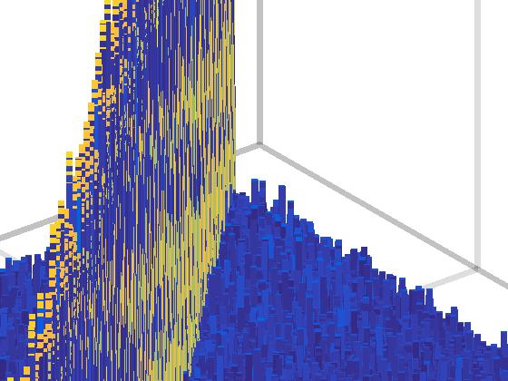
169 (a) G (CS/MIMO) for N t = 12, N r = 4, N p = 8 (b) G (CSTR/MIMO) for N t = 12, N r = 4, N p = 8 Figure 5.6: Comparing G (CS/MIMO) and G (CSTR/MIMO) in 3D plots for Case II with 80% compression ratio 154

170 5.3.2 Coherence in the CSTR/MIMO sensing matrix Recall that the CSTR/MIMO dictionary for transceiver n t and pulse p is given by Eq. (4.17) (see Chapter 4 Section 4.2 for more details). Because every transceiver n t compresses received pulse p with Φ (TR) (n t,p), it follows that the sensing matrix for the CS/MIMO radar in the fusion center is given by [ (Φ Θ (TR) (TR) ) T ( z c = (1,1) Ψ(TR) (TR) T (1,1), Φ (1,N p) Ψ(TR) (1,N p)),, (5.63) ( (TR) ) T ( (TR) ) ] T T Φ (N t,1)ψ(tr) (N,, Φ t,1) (N t,np)ψ(tr) (N, (5.64) t,np) Note that for batch of N p pulses, we assume that the energy normalizing vector g is constant. In other words, for all N p pulses the received energy at N r transceivers is constant. Consequently, the energy normalizing vector g is not dependent to any individual pulse n p. Using Eq. (5.63), the column vector definition of the CSTR/MIMO dictionary Ψ TR (l) for the l th path is given by Ψ (TR) (l) = [ (d((0)t p, 2β l )D(2β (l) )F( t)a(1, τ(θ l ))g) T,, (5.65) (d((1)t p, 2β l )D(2β (l) )F( t)a(2, τ(θ l ))g) T,, (d((n p 1)T p, 2β l )D(2β (l) )F( t)a(n t, τ(θ l ))g) T ] T (Ns N t N p 1). 155

171 Consequently,the measurement matrix for all N t transceivers and N p pulses is given by [ Φ (TR) = (Φ (TR) (1,1) )T,, (Φ (TR) (1,N p) )T, (5.66) (Φ (TR) (2,1) )T,, (Φ (TR) (N t,np))t ] T (Nc N t N p N s N t N p ), which implies the l th column of the CSTR/MIMO sensing matrix is Θ (TR) z c (l) = Φ (TR) Ψ (TR) (l) (N c N t N p 1). (5.67) Inserting Eq. (5.65) and Eq. (5.66) into Eq. (5.67) yields [ Θ (TR) z c (l) = (d((0)t p, 2β l )Φ (TR) (1,1) D(2β (l))f( t)a(1, τ(θ l ))g) T,, (5.68) (d((n p 1)T p, 2β l )Φ (TR) (1,N p) D(2β (l))f( t)a(1, τ(2θ l ))g) T, (d((1)t p, 2β l )Φ (TR) (2,1) D(2β (l))f( t)a(2, τ(2θ l ))g) T,, (d((n p 1)T p, β l )Φ (TR) (N t,np)d(β (l))f( t)a(n t, τ(θ l ))g) T ] T (Nc N t N p 1), Note that in Eq. (5.68), the output of transceiver n t for path l is modeled as a vector given by (T R) γ (l,n,np)(t) d((n p 1)T p, 2β l )Φ (TR) t (n,np)d(2β (l))f( t)a(n r t, τ(θ l ))g (N c 1), (5.69) 156

172 which is compressed by measurement matrix Φ (TR) (n t,np). Inserting Eq. (5.69) into Eq. (5.68) yields [ ( ) T ( ) T Θ (TR) z c (l) = γ (TR) (l,1,1) (t),, γ (TR) (l,1,n (t) p), (5.70) ( γ (TR) (l,2,1) (t) ) T,, ( γ (TR) (l,n t,np)(t) ) T ] T (N c N t N p 1). Note that the output energy of every transceiver n (T R) t for pulse n p, i.e. γ (l,n,np)(t), t depends on energy normalizer vector g which is dependent on the number, position, reflection coefficient, speed, etc. of backscatters situated at path l. Consequently, every column of sensing matrix Θ (TR) z c (l) has a different norm due to energy normalizer vector g. For the CSTR/MIMO gram matrix be comparable with the ( ( )) CS/MIMO gram matrix, we use κ = max diag (Θ (TR) z c ) H Θ (TR) z c to derive the CSTR/MIMO gram matrix G (CSTR/MIMO) = 1 κ (Θ (TR) z c ) H Θ (TR) z c (L L). (5.71) Using the definition of sensing matrix Θ (TR) z c (l) given in Eq. (5.67), every (l, l ) element of the CSTR/MIMO Gram matrix is a scalar given G (CSTR/MIMO) (l, l ) = 1 ( Θ (TR) z κ c (l) ) H Θ (TR) z c (l ). (5.72) 157

173 Inserting Eq. (5.70) into Eq. (5.72) results in G (CSTR/MIMO) (l, l ) = 1 N t N p ( ) H κ γ (TR) (l,n (t) (C) t,n p) γ (l,n,np)(t) n t n t p (5.73) N 1 t N p ( ) H κ γ (TR) (l,n,np)(t) (TR) γ t (l,n,np)(t). t Expanding Eq. (5.73) using Eq. (5.69) gives n t n p G (CSTR/MIMO) (l, l ) 1 N t N p (5.74) κ n n t p ( ) H d((n p 1)T p, 2β l )Φ (TR) (n,np)d(2β (l))f( t)a(n t, τ(θ l ))g t d((n p 1)T p, 2β l )Φ (TR) (n,np)d(2β (l ))F( t)a(n t, τ(θ l ))g. t Reordering terms in Eq. (5.74) yields G (CSTR/MIMO) (l, l ) 1 N t g T (A(n κ t, τ(θ l ))) H (5.75) n t N p (d((n p 1)T p, 2β l )) H d((n p 1)T p, 2β l ) n p Υ {}} (TR) { ( (F( t))h D(2β (l) ) ) ( ) H H Φ (TR) (TR) (n Φ t,np) (n,np)d(2β (l ))F( t) t A(n t, τ(θ l )g). Special case I for G (CSTR/MIMO) : The assumptions used for special case I for G (CSTR/MIMO) are the same as assumptions for for special case I for G (CS/MIMO), i.e., uniform linear array (ULA) with 158

174 d t and d r inter-element spaces for the transmit and receive arrays, respectively. The probing signals F(t) is an orthogonal matrix, i.e., 1 N s (F(t)) H F(t) = I Nt, and there is no signal compression, i.e., N c = N s and Φ (TR) (n t,np) = I N s, then Υ (TR) = I Nt. Expanding Eq. (5.75) using the definition of A(n t, τ(θ l )) yields 1 κ G (CSTR/MIMO) (l, l ) 1 κ N p n p N t n t e jωc(τ n (θ l) τ t n (θ l )) t (5.76) e jωcnp2((βm f β m f )+(βm b β m b ))Tp g T A H (θ l ) INt A H (θ l )g N t n t N r gn 2 r n r N t e jωc(τnt(θl) τnt(θl )) e jωc(τ n (θ l) τ t n (θ l )) t n t N p e jω c2(τ nr (θ l ) τ nr (θ l )) e jωcnp2((βm f β m f )+(βm b β m b ))Tp. n p Assuming g nr = 1, (1 n r N r ), Eq. (5.76) is reduced to G (CSTR/MIMO) (l, l ) g tr (τ(θ l ), τ(θ l ))g tr(τ(θ l ), τ(θ l )) (5.77) g rc (τ(θ l ), τ(θ l ))g d (τ(θ l ), τ(θ l )), where g tr(τ(θ l ), τ(θ l )) = Nt e jωc(τ n (θ l) τ t n (θ l )) t is a periodic sin function and κ = n t Nt 2 N r N p. Comparing Eq. (5.59) and Eq. (5.77) show that the CSTR/MIMO gram matrix derivation contains an extra periodic sinc function which makes off diagonal entries have lower absolute magnitude value as compared to the CS/MIMO gram matrix derivation. In other words in special case I, the CSTR/MIMO sensing matrix has less coherent columns than the CS/MIMO sensing matrix (Fig. 5.3b 159

175 and Fig. 5.4b). However for special case I, both the CS/MIMO gram matrix and the CSTR/MIMO gram matrix do not have a complete incoherent space as there are some off diagonal entries have absolute magnitudes compared to those for the diagonal entries. Special case II for G (CSTR/MIMO) : For special case II, assumptions are orthogonal probing signals, i.e., 1 N s (F(t)) H F(t) = I Nt, and received signals are compressed by sensing matrix, i.e., Φ (C) (n r,n p) (N c N s ) where N c N s. Expanding Eq. (5.75) from the vector-matrix format to the scalar format yields G (CSTR/MIMO) (l, l ) 1 κ N t N p n t N r gn 2 r n r e jω c2(τ nr (θ l ) τ nr (θ l )) (5.78) N t N t e jωc(τn t (θ l) τ nt (θ )) l e jωcnp2((βm f β m f )+(βm b β m b ))Tp e jωc(τ n (θ l) τ t n (θ l )) t n p n t n t e jωc(τ n t (θ l) τ n t (θ l )) Υ (TR) (n t, n p, n t, n t ), where Υ (TR) (n t, n p, n t, n t ) is a scalar representing an element of matrix Υ (TR) (n t, n p ) (N t N t ). To compare the CS/MIMO and CSTR/MIMO sensing matrix coherency, Eq. (5.62) and Eq. (5.78) are used. First, we notice that Υ (TR) (n t, n p ) = Υ (C) (n r, n p ) since both matrices are compressed versions of probing signals F(t) provided the same compression ratio is used. As a result, the magnitude difference between diagonal and non-diagonal entries for both CS/MIMO and CSTR/MIMO gram 160

176 matrices depends on the number of summation terms for Υ (C) (n r, n p, n t, n t ) and Υ (TR) (n t, n p, n t, n t ) where (n t n t ). While for the CS/MIMO gram matrix has N r N p summations Υ (C) (n r, n p, n t, n t ), the CSTR/MIMO gram matrix has N t N p summations for Υ (TR) (n t, n p, n t, n t ). As a result for a fixed number of pulses N p, the coherency of the CS/MIMO and CSTR/MIMO sensing matrices are improved by increasing the number of transceivers on Array B, i.e., N r and Array A,i.e., N t, respectively. The other difference between the CS/MIMO and CSTR/MIMO gram matrix deriva- tions is the extra term Nr n r g 2 n r e jωc2(τnr (θ l ) τ nr (θ l )) which appears in the CSTR/MIMO gram matrix derivation (Eq. (5.78)). Note that (l, l ) pairs are not dependent on gn 2 r which are normalized by applying κ. On the other hand, Nr n r N r n r e jω c2(τ nr (θ l) τ nr (θ l )) amplifies diagonal entries, i.e., l = l and diminishes non-diagonal entries. amplifying and diminishing levels are dependent to the number of transceivers in Array B. Thus, even with the same number of transceivers in Arrays A and B, the CSTR/MIMO sensing matrix is less coherent than CS/MIMO sensing matrix. As a result, the CSTR/MIMO radar system is more compressible and robust for the target parameter estimation. The 161

177 5.3.3 Numerical simulations for the CS/MIMO and the CSTR/MIMO sensing matrices The coherency of CS/MIMO and CSTR/MIMO sensing matrices are studied using Mote Carlo simulations in different setups. Th values of common parameters for all simulation setups are listed in Table 5.2. Inter-element spacing setups in both transceiver arrays A and B are (a) Uniform linear array (ULA); (b) Wide range, random linear array (WR/RLA), and; (3) Narrow range, random linear array (NR/RLA) with the same constraints used for CS/SIMO and CSTR/SIMO radars presented in Subsection Over 1000 Monte Carlo simulation are run for each transceiver pair selection for each inter-element spacing setup. Figures 5.7, 5.8, and 5.9 compares incoherency of CS/MIMO and CSTR/MIMO measurement matrices for ULA, WR/RLA, and NR/RLA inter-element setups, respectively. As simulation results show, the CSTR/MIMO measurement matrix is less coherent than the CS/MIMO measurement matrix for all setups. As a result, the CSTR/MIMO radar system is more compressible and robust for the target parameter estimation than the CS/MIMO radar system. 162

178 Parameter Value Comments F (N s N t ) Random BPSK probing signal g nr ( 2, 3,, 20) Randomly drawn from the set L 9251 Number of dictionary atoms N t (2, 4, 16) Number of transceiver elements in Array A N r (2, 4, 16) Number of transceiver elements in Array B N s 512 Number of samples N c 64 Number of compressed samples N p 20 Number of pulses ω c 2π rad/s Carrier frequency θ mf = θ mb ( 7,, 7 ) DOD and DOA with 0.5 resolution v mf = v mb (300,, 400)m/s Resolution velocity of forward/backward paths with 10m/s NR/RLA spacing (λ/8, λ/2) Inter-element spacing for Narrow Range, Random Linear Arrays (NR/RLA) ULA spacing d nr d nr 1 = λ/2 Inter-element spacing for Uniform Linear Arrays (ULA) WR/RLA spacing (λ/2, 3λ/2) Inter-element spacing for Wide Range, Random Linear Array (WR/RLA) Table 5.2: Parameters used in the simulations for Figs

179 7(G CST R=M IM O ) 7(G CS=M IM O ) No. Transceivers in Array B No. Transceivers in Array A (a) Coherency of CS/MIMO sensing matrix G (CS/MIMO) No. Transceivers in Array B No. Transceivers in Array A (b) Coherency of CSTR/MIMO sensing matrix G (CSTR/MIMO) Figure 5.7: Comparing G (CS/MIMO) and G (CSTR/MIMO) for the ULA setup. 164

180 7(G CST R=M IM O ) 7(G CS=M IM O ) No. Transceivers in Array B No. Transceivers in Array A (a) Coherency of CS/MIMO sensing matrix G (CS/MIMO) No. Transceivers in Array B No. Transceivers in Array A (b) Coherency of CSTR/MIMO sensing matrix G (CSTR/MIMO) Figure 5.8: Comparing G (CS/MIMO) and G (CSTR/MIMO) for the WR/RLA setup. 165

181 7(G CST R=M IM O ) 7(G CS=M IM O ) No. Transceivers in Array B No. Transceivers in Array A (a) Coherency of CS/MIMO sensing matrix G (CS/MIMO) No. Transceivers in Array B No. Transceivers in Array A (b) Coherency of CSTR/MIMO sensing matrix G (CSTR/MIMO) Figure 5.9: Comparing G (CS/MIMO) and G (CSTR/MIMO) for the NR/RLA setup. 166

182 6 Conclusion and Future Work The thesis reviewed a number of parameter estimation approaches for moving targets using the single input multiple outputs (SIMO) and multiple input multiple output (MIMO) radar systems. Such systems perform poorly in the presence of multipath. We applied time reversal (TR) to the MIMO radar systems to improve their estimation accuracy in medium with high multipath due to clutter backscatters. A major problem with the TR/MIMO radar is the large amount of observed data. The ability of the compressive sensing (CS) approach to sample signals at rates below the Nyquist sampling frequency is exploited to reduce the number of observation samples. I have shown that the CS framework can be coupled with TR for parameter estimation in MIMO radars. Applied by itself, the CS/MIMO radar perform poorly in systems with rich multipath due to the coherence of the sensing matrix. On the other hand, the sensing matrix for the CSTR/MIMO is more incoherent leading to superior estimation performance. I have shown analytically that CSTR/SIMO and CSTR/MIMO outperforms CS/SIMO and CS/MIMO 167

183 radar systems, respectively, in terms of both sparsity and coherence measures. Improving coherency enhances the probability of received target backscatters to be sparse for compressive sensing parameter estimation. Improving sparsity increases the robustness of compressibility and parameter estimation. I have validated my analytic derivations using Monte Carlo simulations. Future Work There are several directions in which my research work in the compressive sensing time reversal MIMO radar systems can be extended. Below, I identify three likely directions for the extension of this thesis. 1. Computational time reversal: I have shown that the time reversal (TR) probing increases the performance of the compressive sensing MIMO radar systems. However, the TR approach requires received backscatters to be time reversed, energy normalized and retransmitted back into the medium under investigation. The second transmission implies an increase in power consumption for the compressive sensing TR radar system. References [80, 81] show that TR technique can be applied computationally instead of involving another physical implementation. The computational TR approach uses an estimate of the channel under investigation to eliminate the retransmission step where backscatters are transmitted into the channel. Coupling computational TR approach with compressive sensing approach will eliminate the TR 168

184 probing stage and also save on the power consumption. Additional saving is obtained by not requiring the CSTR/MIMO dictionary. 2. Compressive sensing off the grid: For target parameter estimation, the compressive sensing radar offers a superior alternative to conventional non-compressive systems. But the discretized parameter space associated with the CS step in the CSTR/MIMO radar needs to be designed with a lot of care [82]; (a) If true target parameters do not fall on the finite grid, recorded backscatters cannot often be sparsely represented by the discretized dictionary [83, 84]. (b) Increasing the number of elements (atoms) in the compressive sensing dictionary often leads to numerical instability and increase complexity. Reference [82] proposes a framework in which the compressive sensing dictionary is normalized and continuous. The continuous compressive sensing dictionary (CCSD) can then be applied to compressive sensing MIMO radar systems for estimating parameters associated with the target. Applying the CCSD to time reversal MIMO radar systems would require a CCSD extension to the MIMO radar systems and should be carefully investigated 3. Application to medical imaging: Compressive sensing has been utilized for radar imaging and [85] as well as medical imaging [86]. Previously, I have applied TR based array processing approaches for breast cancer localization 169

185 in magnetic resonance imaging (MRI) [28, 29]. Coupling compressive sensing TR approaches to MRI s for tumour detection is another direction worth pursuing that has the potential of reducing the computational complexity of the localization algorithms by restricting the number of data samples recorded for the MRI. It will also decrease the cost of the MRI machine since a lower rate analog to digital (A/D) sampling card will likely be needed due to the CS step. 170

186 A Unsupervised Time Reversal based Microwave Imaging for Breast Cancer Detection Microwave breast imaging is performed by illuminating the breast tissues with a short pulse of microwaves and processing the reflections (backscatter) to create a pseudospectrum that detects the presence of the breast tumours specifying their locations. An important step in such breast cancer detection techniques is the backscatter pre-conditioning step for effective suppression of the clutter signals arising from scattering mechanisms other than the tumor including the antenna reverberations and reflections from the skin-breast interface and chest wall. The work presented in this appendix proposes a new clutter suppression algorithm that successfully isolates the tumour response from the overall (tumour and clutter) response. The proposed DAF/EDF approach is based on a combination of the data adaptive filter (DAF) and the envelope detection filter (EDF), and does not require any prior training. The DAF/EDF algorithm is then coupled with the time reversal (TR) array imaging approaches [28, 87, 88] and tested by running finite 171

187 difference, time difference (FDTD) electromagnetic simulations based on the magnetic resonance imaging (MRI) data of the human breast. Our results demonstrate the effectiveness of the DAF/EDF algorithm for microwave breast cancer detection. This work has appeared previously in [29]. A.1 Introduction In backscatter imaging, several microwave emitters illuminate the breast and the resulting backscatter waveform is recorded by a specialized antenna array. Malignant breast tumours exhibit significantly different electrical properties from those of the healthy breast tissues [89,90]. Consequently, a cancerous tumour produces a stronger electromagnetic backscatter, which can then possibly be processed using standard array processing approaches to locate the tumour. An important initial step in the breast cancer detection algorithms is backscatter pre-conditioning for effective suppression of the clutter. In the context of breast cancer detection, clutter is defined as signals k c [n] arising from scattering mechanisms other than the tumor, which include the antenna reverberations and reflections from the skin-breast interface and chest wall. Effective suppression of the clutter is necessary to accurately detect and localize the breast tumors. Background subtraction procedures [91] typically used in radar applications for estimating the target response k t [n] from the overall (target and clutter response) k c+t [n] assumes a linear system and requires 172

188 knowledge of the clutter response, i.e., k t [n] = k c+t [n] k c [n]. (A.1) It is, therefore, necessary to have prior knowledge of the response of the normal breast tissues without tumour in an environment identical to the one in which the examination for finding anomalies is later conducted. This is not possible even in screening situations because of the variations in the normal tissues and their growth over time. Therefore, the background subtraction procedure, if used, introduces unwanted distortions in the target response. To decompose the overall response k c+t [n] into the target response k t [n] and the clutter response k c [n] without a training step, we present a filtering algorithm, namely the data adaptive filter/envelope detection filter (DAF/EDF). This is the first contribution of this work. A second problem arises due to multipath, the phenomena in which the backscatter waveform reaches the sensor array via two or more paths. Unlike X-rays, which are non-diffractive and travel in straight lines, microwave propagation in breast tissues is characterized by refraction and multipath effects typically considered detrimental in standard signal processing approaches. Time reversal (TR) offers an alternative paradigm and treats multipath positively by tailoring the received backscatters to the scattering properties of the medium. To overcome the multipath problem, we couple the DAF/EDF clutter suppression algorithm with the 173

189 TR imaging approaches [28, 87, 88]. When tested using the finite difference, time difference (FDTD) electromagnetic simulation environment, derived from the magnetic resonance imaging (MRI) data of the human breast, our approach shows great promise for breast cancer detection. The estimation of the target response in a cluttered medium is considered in [92, 93]. The algorithm proposed in [92] uses matched filter technique to extract the tumour responses. The structure of the algorithm requires a good estimation of the clutter as an input to the algorithm. In addition, the tumour template may be matched to the clutter response and a deterministic solution is not provided to steer the wrong match to the correct match position of the tumour response. DAF [93] also has its own shortcomes which are described in the next section. The appendix is organized as follows. Section A.2 defines the notation and reviews the data adaptive filter [93]. The proposed DAF/EDF algorithm is presented in Section A.3, while Section A.4 presents the detection results based on the electromagnetic breast model [28] derived from an MRI. Finally, Section A.5 concludes the appendix. A.2 The Data Adaptive Filter Algorithm Fig. A.1 shows the setup, comprising of two antenna arrays (Arrays A and B) with equal number N of elements, used for breast cancer detection. The elements 174

190 0 2 Array B 4 6 Array A Skin ε =30 r σ=4.0 S/m Range(cm) 8 10 Breast Tissue ε r =9 σ=0.4 S/m 2 mm Tumour ε r = 50 σ=4 S/m Ribs ε r =12.48 σ= S/m Muscle ε r =55.11 σ= S/m Chest Wall Cross Range(cm) Figure A.1: The EM breast model derived from the MRI of a patient with the proposed antenna geometry (Arrays A and B) parallel to the chest walls. Normally, the antenna arrays are placed well above the breast with the arrays parallel to the chest wall. of Array A are referred to as (1 A i N) and similarly, (1 B i N) for Array B. As each element of Array A probes the breast tissue, all elements in Array B record the mixed backscatter waveforms k (B i) c+t [n] resulting in a (N N) matrix, referred to as the multistatic matrix. Assume that we want to remove the effect of clutter from the first mixed recorded response k (1) c+t[n] recorded at element B 1 of the receiving array, when the first element A 1 in the transmitter 175

191 array probes the reference medium. To estimate the clutter response for the first element, the remaining overall responses [k (2) c+t,, k (N) c+t] recorded when element A 1 probes the medium are used. The data adaptive filter (DAF) [93] assumes a delay of J samples between the probing signal and its clutter response recorded at the neighboring elements of the receiving array. The actual value of the delay J is determined experimentally. To estimate the clutter contribution k c (1) [n] at sample value n of k (1) c+t[n], the following (N 1) vectors of length (2J + 1) are defined 2 i N : b i [n] = [ k (i) c+t[n J],, k (i) c+t[n],, k (i) c+t[n + J]] T. (A.2) By concatenating all vectors b i [n], (2 i N), we get b 2N [n] = [ b T 2 [n],, b T N[n] ] T, (A.3) of length (N 1)(2J +1). By selecting the value of n appropriately, b 2N can be constructed such that it includes the clutter response primarily. The filter coefficients of the DAF are then obtained by solving the following minimization problem min q 2N n 0 +m 1 n=n 0 2 k(1) c+t[n] q T 2N[n]b 2N [n] }{{}, (A.4) ˆk c (1) [n] where q T 2N [n], for (0 n (N 1)(2J +1) 1), is the coefficient filter vector of the DAF. Note that the applied window (n 0 n (n 0 + m 1)) used for the summation operation is picked from a region within the mixed response, which constitute 176

192 primarily of the clutter response. The duration of the window corresponds to the length of clutter response which is determined experimentally through a training step. The LMS solution [93] to Eq. (A.4) is given by q 2N = R 1 p, (A.5) where R = 1 m n 0 +m 1 n=n 0 b 2N [n]b T 2N [n], (A.6) and p = 1 m n 0 +m 1 b 2N [n]k c+t[n]. (1) n=n 0 (A.7) Since the recorded backscatters k (1) c+t[n] with the selected range, (n 0 n n 0 + m 1), are similar in magnitude at all receivers, matrix R is ill-conditioned and, therefore, singular. The inverse of R is computed from its s significant eigenvalues λ s i=1 and the corresponding eigenvectors u s i as follows R s = s i=1 1 λ i u i u T i. (A.8) The clutter artifacts due to skin, breast inhomogeneities, and chest wall can be removed from the n th sample in k (1) c+t using ˆk (1) t [n] = k (1) c+t[n] q T 2N[n]b 2N [n]. (A.9) The above algorithm is repeated for all mixed responses k (i) c+t[n] recorded at different elements of the receiving array when successive elements of the transmitting array 177

193 probes the medium. Likewise, the algorithm is repeated for all other transmitterreceiver pairs to estimate the target response for all pairs. There are certain drawbacks with the DAF approach. First, it requires a training step, where coefficients n 0 and m are determined empirically. Without the training step, there is no way to define the temporal window [n 0,, n 0 + m 1] such that it corresponds only to the clutter. For patients belonging to different age groups and ethnicity, the values of these variables can be quite different. The geometry of Arrays A and B with respect to the breast also affects these values. Further, there is a hidden variable s corresponding to the number of significant eigenvalues, which also varies from one patient to another and is, therefore, difficult to generalize solely from the singular value decomposition (SVD). Next, we propose a new filter based on the DAF, which determines parameters n 0, m, and s without the need of a training step. A.3 The DAF/EDF Algorithm As illustrated in Fig. A.2, the proposed DAF/EDF algorithm consists of the following four steps. 1. Starting Indices n 0 and m: Our simulations show that the starting location of the tumour response k t [n] in the overall response k c+t [n] depends on the geometry of Arrays A and B with respect to the chest wall and the location of the tumour. For example, when both arrays are parallel to the chest wall and 178

194 Figure A.2: The DAF/EDF algorithm. the tumour location is in the middle of the breast, the starting index of the tumour response k t [n] is well after the peak of the clutter reflection. Although the separation of these two signals using this parallel array geometry provides a way to select the starting index n 0 of the temporal window, the relative magnitude of the tumour response compared to the clutter response is low such that it is not recognizable even if the starting index n 0 and length m of the window are known. I propose another geometry for Array A and B which is closer to the breast and parallel to the breast skin (Fig. A.1). Use 179

195 of this geometry makes the magnitude of the tumour response comparable to the clutter response. However, this results in an overlap between the tumour and clutter responses. Our simulations show that there is a delay between the starting indices of the clutter response k c [n] and tumour response k t [n], which can be used to calculate the DAF filter coefficients. Based on our simulations, the delay is never less than 50 samples, which implies m = n Although in our simulations the lower bound for the gap between the skin response and the tumour response is found 50 samples, in reality can be calculated based on an expected value which depends on location of the tumour with respect to the skin and receiver antennas. In order to find the starting index n 0, all mixed responses k c+t [n] are passed through a low pass filter to derive the envelope of the signals. The first peak in the envelope corresponds to the sample where the energy of the signal starts to grow. Since we expect the primary portion of this rise to be related to the clutter because the skin is closer to receiver antennas, the starting index n 0 is given by sample corresponding to the rise. We use Hilbert s algorithm implemented by Kolmogorov [94] for envelope detection. Fig. A.3 shows the output of the envelope detector for the overall response k c+t [n] shown in Fig. A.4(a). 180

196 Figure A.3: The output of the low pass filter on the mixed response to determine n 0 and m parameters. 2. Clutter Signature: For the i th receiver, (2 i N 1), we align and scale the recorded responses k (i 1) c+t and k (i+1) c+t with respect to the peak in k (i) c+t. Note that aligning and scaling only removes the disparity of the channel response at the peak sample for receivers (i 1, i, i + 1) but other samples are still not matched. If the receiver (i 1) and (i + 1) are close enough to the i th receiver, the least mean square (LMS) algorithm can estimate the clutter response for the i th receiver in the temporal window [n 0,, n 0 + m 1] by finding the best fit for the delay J and magnitude of the clutter. The delay J is an independent variable and is related to the inter-antenna spacing and the sampling frequency, which are both instrumental parameters in the 181

197 DAF/EDF algorithm. Note that the delay J in the DAF implementation is determined experimentally. Based on delay J, the input of the LMS algorithm for finding the FIR filter coefficients, which is called the clutter signature for the i th receiver b (i+1) (i 1)[n], is given by (2 i N 1) : b (i+1) (i 1) [n] = [ k (i 1) c+t [n J],, k (i 1) c+t [n + J], (A.10) ] T k (i+1) c+t [n J],, k (i+1) c+t [n + J]. 3. Filter Coefficients: The coefficients of the filter are given by where and q 2i = R 1 p, R = 1 m p = 1 m n 0 +m 1 n=n 0 n 0 +m 1 n=n 0 b (i+1) T (i 1) [n]b(i+1) (i 1) [n], b (i+1) (i 1) [n]k(i) c+t[n]. (A.11) (A.12) (A.13) Since R contains only the clutter response, the pseudoinverse is calculated based on the nonzero eigenvalues. 4. Tumour Response: Apply the filter coefficients estimated in Step 3 to calculate the tumour response using the relationship k (i) t [n] = k c+t[n] (i) q T 2i[n]b (i+1) (i 1) [n]. (A.14) 182

198 Because R contains only the clutter response, there is no need to add additive steps to remove artifacts due to the tumour response in R as is required by the data adaptive filter. As a side note to our discussion, we note that the computational complexity of the proposed DAF/EDF algorithm is the same as DAF approach [93]. Two added steps, i.e. the Hilbert transform and aligning peaks, have lower complexity as compare to the DAF step in the DAF/EDF algorithm. Next, the DAF/EDF algorithm is coupled with the TR array imaging approaches to test the performance of the proposed breast cancer detection algorithm. A.4 Simulations and Results In order to compare the performance of the DAF/EDF algorithm, we use the electromagnetic (EM) finite difference time domain (FDTD) environment to simulate the propagation of the microwave probing signal through breast tissue. The EM model of the breast tissue and the probing signals used are the same as specified in our earlier work [28]. As shown in Fig. A.5, the proposed DAF/EDF based TR algorithm is tested by inserting spherical 2mm tumours at 11 different locations. Additive White Gaussian observation noise (AWN) is added but the signal-to-noise ratio is maintained at 30dB. The results for location 1 are being reported here. Fig. A.4 compares the output (Fig. A.4(b)) of the DAF/EDF algorithm with back- 183

199 ground subtraction (Fig. A.4(c)). Since we have physically inserted the tumour, therefore, we have access to both the tumour-free breast and the one with tumour. Therefore, we can experimentally determine both the overall response k c+t [n] and the clutter response k c [n] for each pair of transmitting and receiving antenna. With A 1 transmitting and B 1 receiving, the target response k t [n] shown in Fig. A.4(b) is obtained by background subtraction and is the ground truth. Fig. A.4(c) is the output of the DAF/EDF algorithm for the same pair {A 1, B 1 } of the antenna arrays. We see that the two estimated target responses are fairly similar in nature. Next, we show that the DAF/EDF estimated target response estimates the tumour location accurately. Fig. A.6 shows that output of the two TR array imaging approaches, namely the TR Adaptive Filter Canceler/Time Reversal Beamforming (TRAIC/TRBF) and the TRAIC/Multiple Signal Classification (TRAIC/MUSIC) as developed in [28, 87,88]. In both cases, the output of the DAF/EDF algorithm is used to determine the target responses. Fig. A.6 shows that the tumour is located with a sufficiently high precision. The DAF/EDF algorithm is, therefore, doing a reasonable job in terms of suppressing the clutter and deriving the target response from the overall response. To test the performance of the performance of the TR approaches with the conventional array imaging approaches such as Direct Subtraction Beam Form- 184

200 ing (DSBF) and Direct Subtraction MUSIC (DS/ MUSIC), Figs. A.7 and A.8 compare the absolute errors for tumour location 1 in the estimated outputs of the four approaches obtained from a Monte Carlo simulation of 1000 runs for tumour location 1 at twp different SNR of 30dB and 15dB. Each vertical line in Figs. A.7 and A.8 represent the mean error value (shown by the middle value) as well as the value of the errors one standard deviation above and below the mean. In this case, we note that the TR approaches outperform their conventional counterparts. Similar results were noted for other tumour locations. A.5 Summary In this appendix, we have shown that the combination of the TR array imaging algorithms and the DAF/EDF algorithm offers a practical approach to detect breast cancer because: (i) it does not need a training stage, and; (ii) it can overcome the multipath distortions commonly observed in microwave breast imaging. Our FDTD simulations show that TR imaging algorithms combined with the DAF/EDF can localize breast tumours with a fairly high accuracy at a variety of SNRs we tested. 185

201 0.1 Amplitude Time (sample) 0.01 (a) k c+t [n]. Amplitude Time (sample) 0.01 (b) k t [n] = k c+t [n] k c [n] obtained by direct subtraction. Amplitude Time (sample) (c) k t [n] estimated by the DAF/EDF algorithm. Figure A.4: Estimated target response obtained from the DAF/EDF approach for tumour in the middle of the breast tissue. 186

202 Range (cm) Cross Range (cm) Figure A.5: A spherical 2mm cancerous tumour is introduced at eleven different locations marked as 1 to 11 in the figure. 187

203 (a) TRAIC/TRBF. (b) TRAIC/MUSIC. Figure A.6: Array imaging pseudospectrum for location 1 and SNR = 30dB obtained from 2 TR array imaging algorithms when tumour response obtained by DAF/EDF algorithm. The tumour location is represented by, while the estimated location is given by. 188