6 Single Sample Methods for a Location Parameter

Transcription

1 6 Single Sample Methods for a Location Parameter If there are serious departures from parametric test assumptions (e.g., normality or symmetry), nonparametric tests on a measure of central tendency (usually the median) are used. Recall: M is a median of a random variable X if P (X M) = P (X M) =.5. The distribution of X is symmetric about c if P (X c x) = P (X c + x) for all x. For symmetric continuous distributions, the median M = the mean µ. Thus, all conclusions about the median can also be applied to the mean. If X be a binomial ( ) random variable with parameters n and p (denoted X B(n, p)) then n P (X = x) = p x (1 p) n x for x = 0, 1,..., n x where ( ) n = x n! x!(n x)! and k! = k(k 1)(k 2) 2 1. Tables exist for the cdf P (X x) for various choices of n and p. The probabilities and cdf values are also easy to produce using SAS or R. Thus, if X B(n,.5), we have ( ) n P (X = x) = (.5) n x x ( ) n P (X x) = (.5) n k k=0 P (X x) = P (X n x) because the B(n,.5) distribution is symmetric. For sample sizes n > 20 and p =.5, a normal approximation (with continuity correction) to the binomial probabilities is often used instead of binomial tables. Calculate z = (x ±.5).5n.5. Use x+.5 when x <.5n and use x.5 when x >.5n. n The value of z is compared to N(0, 1), the standard normal distribution. For example: P (X x) P (Z z) and P (X x) P (Z z) = 1 P (Z z) 6.1 Ordinary Sign Test Assumptions: Given a random sample of n independent observations The measurement scale is at least nominal. Observations can be classified into 2 nonoverlapping categories whose union exhausts all possibilities. The categories will be labeled + and. 88

2 Hypotheses: The inference involves comparing probabilities P (+) and P ( ) for outcomes + and. (A) Two-sided: H 0 : P (+) = P ( ) vs H 1 : P (+) P ( ) (B) Upper one-sided: H 0 : P (+) P ( ) vs H 1 : P (+) < P ( ) (C) Lower one-sided: H 0 : P (+) P ( ) vs H 1 : P (+) > P ( ) Note: H 0 is true only if P (+) = P ( ) =.5 Method: For a given α Let T + = the number of + observations. Let T = the number of observations. If H 0 is true, then we would expect T + and T to be nearly equal ( n/2). In other words, if H 0 is true, T + and T are binomial B(n,.5) random variables. For alternative hypothesis (A) H 1 : P (+) P ( ). Let T = min(t +, T ). Then find the largest t such that B(n,.5) probability P (X t) α/2. (B) H 1 : P (+) < P ( ). Let T = T +. Then find the largest t such that B(n,.5) probability P (X t) α. (C) H 1 : P (+) > P ( ). Let T = T. Then find the largest t such that B(n,.5) probability P (X t) α. Decision Rule For (A), (B), or (C), if T is too small, then we will reject H 0. That is, If T t, Reject H 0. If T > t, Fail to Reject H 0. Large Sample Approximation 1. For the one-sided H 1, calculate z = T n.5 n z = T +.5.5n.5 n for (B) if T + <.5n z = T +.5.5n.5 n for (C) if T <.5n z = T.5.5n.5 n for (B) if T + >.5n for (C) if T >.5n 2. For the two-sided H 1, take the smaller of the two z-values in (1.). 3. Find Φ(z) = P (Z z) from the standard normal distribution. 4. Reject H 0 if (i) if P (Z z) α for either 1-sided test or (ii) P (Z z) α/2 for the 2-sided test. 89

3 90 44

4 Example: (From Gibbons, Nonparametric Methods for Quantitative Analysis). An oil company is considering the following procedures for training prospective service station managers: 1. On-the-job training under actual working conditions for three months. 2. A company-run school training program concentrated over one month. They plan to compare the two procedures in an experiment. No training program can be the only determining factor for the success of a manager. Success is also affected by other factors such as age, intelligence, and previous experience. In order to eliminate the effects of these factors as much as possible, each trainee is matched with another trainee that has similar attributes (such as similar age and previous experience). If a good match does not exist for a trainee, then the trainee is not included in the experiment. Once pairs are determined, one member of each pair is randomly selected to receive the on-the-job training, while the other is assigned to the company school. After completing the assigned training program, the personnel manager assesses each trainee and judges which member of each pair has done a better job of managing the service station. In total, 13 pairs had completed the training programs. The personnel manager stated that for 10 of the 13 pairs, the better manager received the company school training. Is there sufficient evidence to claim that the company-run school training program is more effective? Table of Binomial Probabilities and Binomial CDF for n=13, p=.5 n p x f(x) = Pr(X=x) F(x) = Pr(X<=x) < <.025 < > Sign (Binomial) Test for Location Assumptions: Given a random sample of n independent observations x 1, x 2,..., x n : The variable of interest is continuous, and the measurement scale is at least ordinal. Hypotheses: The inference concerns a hypothesis about the median M of a single population. (A) Two-sided: H 0 : M = M o vs H 1 : M M o (B) Upper one-sided: H 0 : M = M o vs H 1 : M > M o (C) Lower one-sided: H 0 : M = M o vs H 1 : M < M o 91

5 Method: For a given α Let T + = the number of observations > M o. Let T = the number of observations < M o. Delete any x i = M o and adjust the sample size n accordingly. If H 0 is true, then T + and T are binomial B(n,.5) random variables. Thus, we would expect T + and T to be approximately equal ( n/2). For alternative hypothesis (A) H 1 : M M o. Let T = min(t +, T ). Then find the largest t such that B(n,.5) probability P (X t) α/2. (B) H 1 : M > M o. Let T = T. Then find the largest t such that B(n,.5) probability P (X t) α. (C) H 1 : M < M o. Let T = T +. Then find the largest t such that B(n,.5) probability P (X t) α. Perform the Ordinary Sign Test based on T and t. Decision Rule For (A), (B), or (C), if T is too small, then we will reject H 0. That is, If T t, Reject H 0. If T > t, Fail to Reject H 0. Large Sample Approximation Same as for the Ordinary Sign Test. Example 2.1 from Applied Nonparametric Statistics by W. Daniel. In a study of heart disease, a researcher measured the blood s transit time in subjects with healthy right coronary arteries. The median transit time was 3.50 seconds. In another study, the researchers repeated the transit time study but on a sample of 11 patients with significantly blocked right coronary arteries. The results (in seconds) were Can these researchers conclude (using α =.05) that the median transit time in the population of patients with significantly blocked right coronary arteries is different than 3.50 seconds? 2. Can these researchers conclude (α =.05) that the median transit time in the population of patients with significantly blocked right coronary arteries is less than 3.50 seconds? 92

6 Table of Binomial Probabilities and Binomial CDF for n=10, p=.5 n p x f(x) = Pr(X=x) F(x) = Pr(X<=x) < <-- < Special Case: Paired Data Assumptions: Given a random sample of n independent pairs of observations (x 1, y 1 ), (x 2, y 2 ),..., (x n, y n ) : Both variables X and Y are continuous, and the measurement scales are at least ordinal. Testing Procedure: Calculate all differences D i = y i x i for i = 1,..., n. Use the median difference M D in the hypotheses. Typically, M D = 0. Run the Sign Test based on the differences (the D i values). Example 4.1 from Applied Nonparametric Statistics by W. Daniel. Researchers studied the effects of togetherness on the heart rate in rats. They recorded the heart rates of 10 rats while they were alone and while in the presence of another rat. The results are shown below. Using an α =.05 significance level for the Sign Test, can we conclude that togetherness increases the heart rate in rats? For this data, the ten D i values are

7 6.2.2 Sign Test Examples using R and SAS R Output for Sign (Binomial Test Examples) > # Sign Test Example from Gibbons > binom.test(10,13) Exact binomial test number of successes = 10, number of trials = 13, p-value = <-- Fail to reject alternative hypothesis: true probability of success is not equal to percent confidence interval: <-- The CI contains.5 so we fail to reject Ho sample estimates: probability of success > # Sign (Binomial) Test for Location -- Daniel Ex. 2.1 > time <- c(1.80,3.30,5.65,2.25,2.50,3.50,2.75,3.25,3.10,2.70,3.00) > time = time > time [1] > ties = sum(time==0) > ties [1] 1 > binom.test(sum(time>0),length(time)-ties) Exact binomial test Reject Ho ^^^ number of successes = 1, number of trials = 10, p-value = alternative hypothesis: true probability of success is not equal to percent confidence interval: <--.5 is not in the CI, so reject Ho sample estimates: probability of success 0.1 > # Sign (Binomial) Test for Location -- Paired Data, Daniel Ex. 4.1 > alone <- c(463,462,462,456,450,426,418,415,409,402) > together <- c(523,494,461,535,476,454,448,408,470,437) > diff <- together - alone > ties = sum(diff==0) > ties [1] 0 > binom.test(sum(diff>0),length(diff)-ties) 94

8 Exact binomial test Fail to reject Ho ^^^^^^^ number of successes = 8, number of trials = 10, p-value = alternative hypothesis: true probability of success is not equal to percent confidence interval: sample estimates: probability of success 0.8 R Code for Sign (Binomial Test Examples) # Sign Test Example from Gibbons binom.test(10,13) # Sign (Binomial) Test for Location -- Daniel Ex. 2.1 time <- c(1.80,3.30,5.65,2.25,2.50,3.50,2.75,3.25,3.10,2.70,3.00) time = time time ties = sum(time==0) ties binom.test(sum(time>0),length(time)-ties) # Sign (Binomial) Test for Location -- Paired Data, Daniel Ex. 4.1 alone <- c(463,462,462,456,450,426,418,415,409,402) together <- c(523,494,461,535,476,454,448,408,470,437) diff <- together - alone ties = sum(diff==0) ties binom.test(sum(diff>0),length(diff)-ties) SAS Output for Sign (Binomial) Test Examples In SAS, the Sign (Binomial) Test statistic is denoted M, and it represents the deviation in the observed count T + from the expected count.5n when the null hypothesis is true. Ordinary Sign Test for Training Program Example The UNIVARIATE Procedure Variable: level Tests for Location: Mu0=0 Test -Statistic p Value Student s t t Pr > t Sign M -3.5 Pr >= M <-- Fail to Signed Rank S Pr >= S reject Ho 95

9 Sign (Binomial) Test for Example 2.1 Variable: diff Basic Statistical Measures Location Variability Mean Std Deviation Median Variance Tests for Location: Mu0=0 Test -Statistic p Value Student s t t Pr > t Sign M -4 Pr >= M <-- Reject Signed Rank S Pr >= S Ho Sign (Binomial) Test for Paired Differences -- Example 4.1 Obs alone together diff Variable: diff Basic Statistical Measures Location Variability Mean Std Deviation Median Variance Tests for Location: Mu0=0 Test -Statistic p Value Student s t t Pr > t Sign M 3 Pr >= M <--- Fail to Signed Rank S 24.5 Pr >= S reject Ho 96

10 SAS Code for Sign (Binomial) Test Examples DM LOG; CLEAR; OUT; CLEAR; ; OPTIONS NODATE NONUMBER LS=76 PS=54; ****************************************************************; *** Ordinary Sign Test: Let -1,1 represent the 2 categories. ***; *** The frq values are the category frequencies ***; ****************************************************************; DATA in; INPUT level LINES; DATA signtest (DROP=i); SET in; IF level = -1 THEN DO i = 1 TO frq; OUTPUT; end; IF level = 1 THEN DO i = 1 TO frq; OUTPUT; end; PROC UNIVARIATE DATA=signtest; VAR level; TITLE Ordinary Sign Test for Training Program Example ; ******************************************; *** Sign (Binomial) Test for Location: ***; **** Example 2.1 in course notes ***; ******************************************; DATA in2; med_time = 3.50; INPUT diff = time - med_time; OUTPUT; LINES; PROC UNIVARIATE DATA=in2; VAR diff; TITLE Sign (Binomial) Test for Example 2.1 ; RUN; ****************************************************; *** Sign (Binomial) Test for Paired Differences: ***; *** Example 4.1 in course notes ***; ****************************************************; DATA in3; INPUT alone diff = together - alone; OUTPUT; LINES; ; PROC PRINT DATA=in3; TITLE Sign (Binomial) Test for Paired Differences -- Example 4.1 ; PROC UNIVARIATE DATA=in3; VAR diff; RUN; 97

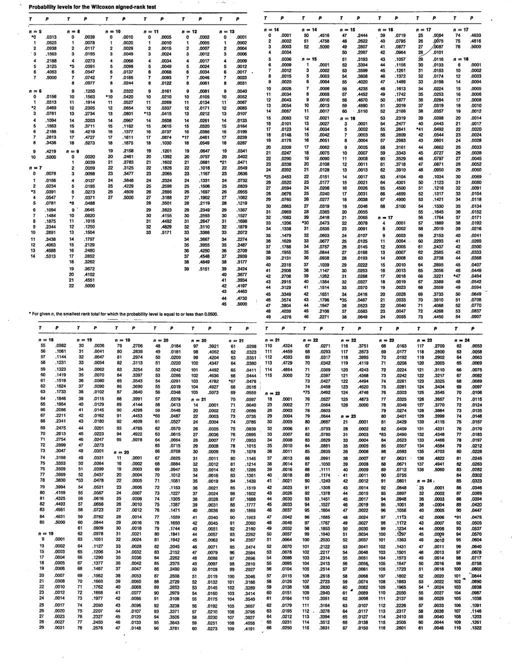
11 6.3 Wilcoxon Signed Rank Test Assumptions: Given a random sample of n independent observations X 1,..., X n : Each X i was drawn from a symmetric and continuous population. Each X i has the same median M for i = 1,..., n). The measurement scale is at least on the interval scale. Hypotheses: The inference concerns a hypothesis about the median M of a single population. Given M o, a hypothesized value of the median, we have: (A) Two-sided: H 0 : M = M o vs H 1 : M M o (B) Lower one-sided: H 0 : M = M o vs H 1 : M < M o (C) Upper one-sided: H 0 : M = M o vs H 1 : M > M o Because of the symmetry assumption, we can replace the median M with the mean µ in the hypotheses. Method: For a given α Calculate all differences D i = X i M o. Remove all cases having D i = 0 and adjust the sample size n accordingly. Assign ranks 1, 2,..., n to the D i. For tied D i values, assign average ranks. If H 0 is true, then the D i are symmetrically distributed about 0. That is, we expect (Ranks where Di > 0) (Ranks where D i < 0). Let T + = (R i when D i > 0) and T = (R i when D i < 0). Under H 0, the sampling distributions of T + and T are symmetric about n(n + 1)/4 and can assume integer values from 0 to n(n + 1)/2. Note that T = n(n + 1)/2 T +. For alternative hypothesis: (A) (B) (C) H 1 : M M o, let T = min(t +, T ). Let w be the largest value from the Wilcoxon Signed Rank Test Table such that P (T w) α/2. H 1 : M < M o, let T = T +. Let w be the largest value from the Wilcoxon Signed Rank Test Table such that P (T w) α. H 1 : M > M o, let T = T. Let w be the largest value from the Wilcoxon Signed Rank Test Table such that P (T w) α. Decision Rule If T w, Reject H 0. If T > w, Fail to Reject H 0. 98

12 Large Sample Approximation (with continuity correction) (n > 30) Computer packages like R and SAS calculate approximate p-values for the two-sided alternative H 1 based on large sample normal distribution approximations. The normalizing formula is: T T n(n + 1)/4 = = T E(T ). n(n + 1)(2n + 1)/24 V ar(t ) Daniel (Applied Nonparametric Statistics, page 42) describes an adjustment to this formula in the event of ties. Example of Wilcoxon Signed Rank Test A random sample of 12 fish was taken and the bodyweights recorded. Test the null hypothesis H 0 : µ = 3.0 against the alternative H 1 : µ < 3.0 pounds. (Assume they are sampled from the same symmetric distribution.) R code for Wilcoxon Signed Rank Test with Confidence Interval # Wilcoxon Signed Rank Test with Confidence Interval for Fish Data fish <- c(2.11,2.22,2.23,2.41,2.54,2.73,2.80,2.80,2.92,3.06,3.12,3.12) wilcox.test(fish,mu=3,conf.int=true) R output for Wilcoxon Signed Rank Test with Confidence Interval > # Wilcoxon Signed Rank Test with Confidence Interval for Fish Data > fish <- c(2.11,2.22,2.23,2.41,2.54,2.73,2.80,2.80,2.92,3.06,3.12,3.12) > wilcox.test(fish,mu=3,conf.int=true) Wilcoxon signed rank test with continuity correction data: fish V = 8, p-value = alternative hypothesis: true location is not equal to 3 95 percent confidence interval: sample estimates: (pseudo)median SAS code and selected output: SIGN TEST AND WILCOXON SIGNED RANK TEST The UNIVARIATE Procedure Basic Statistical Measures Location Variability Mean Std Deviation Median Variance Mode Range Interquartile Range

13 Tests for Location: Mu0=0 Test -Statistic p Value Student s t t Pr > t Sign M -3 Pr >= M Signed Rank S -31 Pr >= S <-- p-value The Signed Rank statistics S in SAS = T (n(n + 1)/4 = 8 (12)(13)/4 = 8 39 = 31. The p-value is based on the normal approximation and is for a two-sided alternative. Thus, for one-sided H 1 : M < 3.0, the approximate p-value =.0112/2 = OPTIONS LS=72 PS=60 NONUMBER NODATE; DATA IN; INPUT X=X-3; CARDS; PROC UNIVARIATE DATA=IN; VAR X; TITLE ONE SAMPLE TESTS FOR LOCATION: ; TITLE2 SIGN TEST AND WILCOXON SIGNED RANK TEST ; RUN; Reference Distribution for the Signed Rank Test (n = 5) If H 0 is true, then any random D i has a probability 1/2 of being > M o or < M o. Without loss of generality, let D 1, D 2, D 3, D 4, D 5 be ordered from smallest to largest. Then when n = 5, every possible ranking of D 1, D 2, D 3, D 4, D 5 has a (1/2) 5 = 1/32 chance of occurring. Possible Ranks Cumulative T + With D i > 0 Probability Probability 0 None 1/32 1/32 = /32 2/32 = /32 3/32 = or 1,2 2/32 5/32 = or 1,3 2/32 7/32 = or 1,4 or 2,3 3/32 10/32 = ,5 or 2,4 or 1,2,3 3/32 13/32 = ,5 or 3,4 or 1,2,4 3/32 16/32 = ,5 or 1,2,5 or 1,3,4 3/32 19/32 = ,5 or 1,3,5 or 2,3,4 3/32 22/32 = ,4,5 or 2,3,5 or 1,2,3,4 3/32 25/32 = ,4,5 or 1,2 3,5 2/32 27/32 = ,4,5 or 1,2 4,5 2/32 29/32 = ,3,4,5 1/32 30/32 = ,3,4,5 1/32 31/32 = ,2,3,4,5 1/32 32/32 = 1 100

14 101 56

15 57102

16 6.3.2 Special Case: Paired Data Assumptions: Given a random sample of n pairs of observations (x 1, y 1 ), (x 2, y 2 ),..., (x n, y n ). Let D i = y i x i for i = 1,..., n. The D i s are independent. The measurement scale is at least on the interval scale. The distribution of the differences D i = y i x i for i = 1,..., n is symmetric. Testing Procedure: Calculate all differences D i = y i x i for i = 1,..., n. Use the median difference M D in the hypotheses. Typically, M D = 0. Because of the symmetry assumption, we can replace the median M D with the mean µ D in the hypotheses. Run the Wilcoxon Signed Test based on the D i. Example of Wilcoxon Signed Rank Test for Paired Data Two judges were asked to independently rate the rehabilitative potential for each of 22 male prison inmates. The following table contains the ratings: Inmate (i) Judge 1 Judge 2 D i D i Sign R i remove tie remove tie

17 SAS code and output: DATA IN; DO INMATE=1 TO 22; INPUT JUDGE1 JUDGE2 DIFF = JUDGE1 - JUDGE2; OUTPUT; END; CARDS; ; PROC UNIVARIATE DATA=IN; VAR DIFF; TITLE WILCOXON SIGNED RANK TEST FOR PAIRED DATA ; RUN; ==================================================================== WILCOXON SIGNED RANK TEST FOR PAIRED DATA The UNIVARIATE Procedure Variable: DIFF Tests for Location: Mu0=0 Test -Statistic p Value Student s t t Pr > t Sign M 5 Pr >= M Signed Rank S 75 Pr >= S <-- Reject Ho The approximate p-value is Thus, we would reject the null hypothesis H o : M D = Confidence Interval for the Median Based on the Wilcoxon Signed Rank Test To find the point estimate for the median M: Calculate all paired averages u ij allowing replication: u ij = x i + x j. 2 There are ( ) ( n 2 + n = n+1 ) 2 such averages. Arrange the u ij in increasing order. The point estimate for M is M = the median of the {u ij }. Method: For an approximate confidence level 100(1 α)% : Use the Wilcoxon Signed Rank Test Table to find the largest t such that P (T t) α/2. Let M L = (t + 1) st u ij observation from the beginning and M U = (t + 1) st u ij observation from the end of the set of ordered u ij values. Statistically, P (M L M M U ) = P (t + 1 T n(n + 1)/2 t) where T is the Wilcoxon signed rank statistic. The approximate 100(1 α)% confidence interval is (M L, M U ). The exact confidence level for (M L, M U ) is determined by the distribution given in the Wilcoxon Signed Rank Test Table. That is, if p = P (X t), then (M L, M U ) is an exact 100(1 2p)% confidence interval for M. 104

18 Note: You do not need to calculate all of the u ij values, but only the (t + 1) st largest and smallest. This procedure is also known as the Hodges-Lehmann estimates of shift. Example of Hodges-Lehmann confidence interval for M A random sample of 12 fish was taken and the body weights were recorded Calculate an approximate 95% confidence interval for the median bodyweight M. For n = 12, the largest value in the Wilcoxon Signed Rank Test Table with P (T t).025 is t = 13. Note: P (T 13) = Then t + 1 = 14 and n(n + 1)/2 t = = 65. Now find the 14 th and 65 th values in the list of the 78 u ij values. HODGES-LEHMANN CONFIDENCE INTERVAL Obs x1 x2 u Obs x1 x2 u <-- lower endpoint <-- upper endpoint Thus, the confidence interval is (2.42,2.93). 105

19 R code for Wilcoxon Signed Rank Test with Confidence Interval # Wilcoxon Signed Rank Test with Confidence Interval for Fish Data fish <- c(2.11,2.22,2.23,2.41,2.54,2.73,2.80,2.80,2.92,3.06,3.12,3.12) wilcox.test(fish,mu=3,conf.int=true) R output for Wilcoxon Signed Rank Test with Confidence Interval Wilcoxon signed rank test with continuity correction data: fish V = 8, p-value = alternative hypothesis: true location is not equal to 3 95 percent confidence interval: <--- Approximate 95% confidence interval for mu is (2.42, 2.93) sample estimates: (pseudo)median Asymptotic Relative Efficiency (A.R.E.) One way to compare properties of statistical tests is to compare the efficiency properties. The definition of efficiency can vary but, generally speaking, it is used to compare the sample size required of one test with that of another test under similar conditions. Suppose that two tests may be used to test a particular H 0 against a particular H 1, and both tests have the same specified α and β errors. These tests are therefore comparable under conditions related to the level of significance α and power (1 β). Thus, the test requiring the smaller sample size to satisfy these conditions will have the smaller sampling cost and effort. That is, the test with the smaller required sample size is more efficient than the other test, and its relative efficiency is greater than one. Let T 1 and T 2 represent two tests that test the same H 0 against the same H 1 with the same specified α and β values. For example, T 1 is the Sign Test and T 2 is the Wilcoxon Signed Rank Test which are used to test H 0 : µ = µ 0 with α =.05 and power 1 β =.90. The relative efficiency of test T 1 with respect to test T 2 is the ratio n 2 /n 1, where n 1 is the required sample size of T 1 to equal the power of test T 2 which has sample size n 2 (assuming the same H 0 and significance level α). Thus, there is a relative efficiency of T 1 with respect to T 2 for each choice of α and n 2. A more general measure of efficiency (asymptotic relative efficiency) was developed. Consider the situation of letting sample size n 1 increase for T 1 with specified α and β. Then there exists a sequence of n 2 values, such that for each value of n 1 (n 1 ), T 2 has the same α and β values. In other words, there is a sequence of relative efficiency values n 2 /n 1. If n 2 /n 1 approaches a constant value as n 1, and, if that constant is the same for all choices of α and β, then the constant is called the asymptotic relative efficiency of T 1 with respect to T

20 Note that if the A.R.E. exists for T 1 and T 2, then the limiting A.R.E. value is independent of the choice of α and β. To select a test with superior power, we generally select the test with the greatest A.R.E. because the power depends on many factors such as the maximum number of observations that can be collected given experimental or sampling resources and the type of distribution that generates the data (normal?, weibull?, gamma?,...) which is usually unknown. The A.R.E. is, in general, difficult to calculate. In this course, we will only consider A.R.E. results for various pairs of tests and for several choices of distributions. Note that A.R.E. assumes that an infinite sample size can be taken. Thus, a natural question arises: How good is a measure assuming an infinitely large sample when most practical situations involve relatively small sample sizes? In an attempt to answer this question, studies of exact relative efficiency values for very small samples have shown that A.R.E. provides a good approximation to the relative efficiency in many situations of practical interest A.R.E. Comparison for Three Single-Sample Tests of Location We will compare the t-test, Sign test, and the Wilcoxon Signed Rank test using the A.R.E. values. To do this we will consider three situations involving symmetric distributions. Under symmetry assumptions, H 0 and H 1 are identical for all three tests. (I) The sample was randomly sampled from a normal distribution having density function ] 1 f(x; µ, σ) = [ σ 2π exp (x µ)2 for < x < 2σ 2 Without loss of generality, we can assume it is a standard normal N(0, 1) having density function φ(x) = 1 2π exp ( x 2 /2 ) for < x < (II) The sample was randomly sampled from a uniform distribution having density function: f(x; a, b) = 1 (b a) for a < x < b = 0 otherwise Without loss of generality, we can assume a uniform U(0, 1) having density function f(x) = 1 for 0 < x < 1 = 0 otherwise The uniform distribution is considered a light-tailed symmetric distribution. 107

21 f(x) = 1 for 0 < x < 1 = 0 otherwise The uniform distribution is considered a light-tailed symmetric distribution. (III) The sample was randomly sampled from a double exponential distribution (DE) having Thedensity samplefunction was randomly sampled from a double exponential distribution (DE) hav- (III) ing f(x; a, b) = 1 ( ) 2b exp x a for < x < f(x; a, b) = 1 ( ) 2b exp x a for < x < b Without loss of generality, we can assume DE(0, 1) having density function Without loss of generality, assume it is DE(0, 1) having density function f(x) f(x) = exp ( x ) 1 exp ( x ) for 2 for < x < The DE distribution is is a heavy-tailed symmetric distribution. Table of A.R.E. Values 61 Test (I) Normal (II) Uniform (III) Double Exponential Comparison Distribution Distribution Distribution Sign test 2/π / / vs t-test (t) (t) (Sign) Wilcoxon Signed Rank test 3/2 = /4 = vs Sign test (Wlcxn) (Wlcxn) (Sign) Wilcoxon Signed Rank test 3/π /2 = vs t-test (t) (=) (Wlcxn) Bold-face letters indicate which test is more efficient 6.5 Introduction to the One-Sample Randomization Test Paired Data Example: An experimental drug was tested on 7 subjects. Blood level measurements were taken before (X) and after (Y ) administering the drug. In this situation, we have paired data. The difference (D = Y X) in blood level measurements for each subject were: Di Patient i D Difference D i The goal is to test the hypothesis that there is no change in blood level measurement after taking the drug. Statistically, we will assume that the distribution of the difference in blood levels measurements under the null hypothesis H 0 is symmetric about

22 Thus, H 0 : µ D = 0. We will consider two possible alternatives: (1) H 1 : µ D 0 and (2) H 1 : µ D < 0. If H 0 is true (and assuming symmetry about 0), the signs (+ or ) of the 7 measurements can be considered random. For example, we could have just as likely observed Di Patient i D Difference D i or Di Patient i D Difference D i or any other randomization of the signs. The Randomization Reference Distribution 1. Consider all possible sign assignments or randomizations of signs for the seven differences. 2. Calculate D i for each randomization. In this example, there are 2 7 = 128 different randomizations of the seven signs. This yields the randomization distribution of D i. In terms of testing, it is statistically equivalent to use the randomization distribution of the mean D. 3. Now compare the OBSERVED D i =.664 to the randomization distribution to find the probability (p-value) associated with the test H 0 : µ D = 0 against the alternative H 1 hypothesis. Case 1: For alternative H 1 : µ D 0, from the randomization reference distribution we see the p-value = P ( D i.664 ) = P (D i.664 ) + P (D i.664 ) = (6 + 6)/128 = Case 2: For alternative H 1 : µ D < 0, from the randomization reference distribution we see the p-value = P (D i.664 ) = 6/128 =

23 RANDOMIZATION TEST #1 Obs ID1 ID2 ID3 ID4 ID5 ID6 ID7 D_SUM CDF < RANDOMIZATION TEST #1 Obs ID1 ID2 ID3 ID4 ID5 ID6 ID7 D_SUM CDF <

24 SAS Code to Generate the Randomization Distribution for the Change in Blood Level Measurements DM LOG;CLEAR;OUT;CLEAR; ; OPTIONS LS=72 PS=68 NONUMBER NODATE; DATA IN; INPUT CARDS; DATA IN; SET IN; DO I1=-1 TO 1 BY 2; ID1=I1*D1; DO I2=-1 TO 1 BY 2; ID2=I2*D2; DO I3=-1 TO 1 BY 2; ID3=I3*D3; DO I4=-1 TO 1 BY 2; ID4=I4*D4; DO I5=-1 TO 1 BY 2; ID5=I5*D5; DO I6=-1 TO 1 BY 2; ID6=I6*D6; DO I7=-1 TO 1 BY 2; ID7=I7*D7; D_SUM = SUM(OF ID1-ID7); OUTPUT; END; END; END; END; END; END; END; KEEP ID1-ID8 D_SUM; PROC SORT DATA=IN; BY D_SUM; DATA IN; SET IN; CDF=_N_/128; PROC PRINT DATA=IN; TITLE RANDOMIZATION TEST #1 ; RUN; Randomization Test for Paired Data Assumptions: Given a random sample of n pairs of observations (x 1, y 1 ), (x 2, y 2 ),..., (x n, y n ). The differences D i = y i x i are independent. The distribution of each D i is symmetric and has the same mean. The measurement scale for the D i s is at least interval. Hypotheses: The inference concerns a hypotheses about whether or not the mean difference µ D = 0: (A) Two-sided: H 0 : µ D = 0 vs H 1 : µ D 0 (B) Lower one-sided: H 0 : µ D = 0 vs H 1 : µ D < 0 (C) Upper one-sided: H 0 : µ D = 0 vs H 1 : µ D > 0 Because of the symmetry assumption, we can replace the mean difference µ D with the median difference M D in the hypotheses. Method: For a given α Calculate the sum D i for each of the possible 2 n sign randomizations. Order these values to form the randomization distribution for the D i. 111

25 Decision Rule For (A) H 1 : µ D 0, If ACTUAL D i < 0, let D = D i. If ACTUAL D i > 0, let D = D i. For (B) H 1 : µ D < 0, let D = D i. For (C) H 1 : µ D > 0, let D = D i. p value = 2 Number of D is D 2 n p value = Number of D is D 2 n p value = Number of D is D 2 n = Number of D i s D 2 n Reject H 0 if p-value α. Otherwise, we fail to reject H 0. Without loss of generality, you can replace D i with D in the preceding arguments. Note that the number of sign randomizations (2 n ) forming the randomization distribution grows rapidly. For example, when n = 20, there are over 1 million randomizations. In such cases, it is generally not feasible to generate the entire randomization distribution. To handle this problem, a large number of randomizations of the signs are randomly taken. Then, an approximate randomization distribution is generated from this large subset of possible randomizations. Approximate p-values can then be determined from this distribution. This is known as the monte-carlo approach to generating approximate p-values. The following R code will generate p-values using the monte-carlo approach for the single-sample Randomization Test for Location. R Code for Randomization Test on Paired Data (Differences) # Single Sample Randomization Test for Location # Enter the number of permutations to take Prep = Prep # Enter vector of differences D <- c(-.187,.011,-.250,.034,-.137,-.112,-.023) D # Calculate the mean difference meand <- mean(d) meand sgnd <- sign(meand) Fp = 0 112

26 upper <- 0 lower <- 0 n = length(d) # Begin sign randomizations meanpermd <- 1:Prep for (i in 1:Prep){ sgnvec <- sign(runif(n)-.5) permvec <- sgnvec*d # random vector with 1 or -1 values } # Calculate the mean difference for the i_th randomization vector meanpermd[i] <- mean(permvec) if(meanpermd[i]>=meand) upper = upper+1 if(meanpermd[i]<=meand) lower = lower+1 # Calculate p-values: # for lower one-sided Ho pval_lower <- lower/prep pval_lower # for upper one-sided Ho p-val_upper <- upper/prep pval_upper # for two-sided Ho if(sgnd < 0) pval_two_sided = if(sgnd > 0) pval_two_sided = pval_two_sided 2*pval_lower 2*pval_upper hist(meanpermd) R Output for Randomization Test on Paired Data > meand > # Calculate p-values: > # for lower one-sided Ho [1] > # for upper one-sided H0 [1] > # for two-sided Ho [1] Note that the p-values from the monte-carlo approach (.04644,.96076,.09288) approximate the exact p-values of ( , ,.09375) from the true randomization distribution. Without loss of generality, I used D instead of D i in my R code. 113

27 Histogram ofhistogram 50,000 Values of meanpermd using the Monte-Carlo Approach Frequency meanpermd Single Sample Randomization Test for H o : µ = µ 0 Suppose we want to perform a randomization test if our inference concerns a hypotheses about whether or not µ = µ0 for some specified value µ 0 against one of three alternatives: (A) Two-sided: H 0 : µ = µ 0 vs H 1 : µ µ 0 (B) Lower one-sided: H 0 : µ = µ 0 vs H 1 : µ < µ 0 (C) Upper one-sided: H 0 : µ = µ 0 vs H 1 : µ > µ 0 To perform a randomization test, simply subtract µ 0 from each observation, and then run the randomization test as you would for paired data. Example: A random sample of 12 fish was taken and the bodyweights recorded. Test the null hypothesis H 0 : µ = 3.0 against the alternative H 1 : µ < 3.0 pounds Based on the randomization test, the p-value is approximately Therefore, we would reject H 0 : µ = 3.0 and conclude that µ < 3.0 pounds. 114

28 R Code for Randomization Test for Fish Weight Data # Single Sample Randomization Test for Location # Enter the number of randomizations to take Prep = Prep fish <- c(2.11,2.22,2.23,2.41,2.54,2.73,2.80,2.80,2.92,3.06,3.12,3.12) # Enter the hypothesized mean mu0 = 3 # Enter vector of differences D <- fish - mu0 D <-- enter mu_0 <- subtract mu_0 from the data # Calculate the mean difference meand <- mean(d) meand sgnd <- sign(meand) Fp = 0 upper <- 0 lower <- 0 n = length(d) # Begin sign randomizations meanpermd <- 1:Prep for (i in 1:Prep){ sgnvec <- sign(runif(n)-.5) permvec <- sgnvec*d # random vector with 1 or -1 values # Calculate the mean difference for the i_th randomization vector meanpermd[i] <- mean(permvec) if(meanpermd[i]>=meand) upper = upper+1 if(meanpermd[i]<=meand) lower = lower+1 } # Calculate p-values: # for lower one-sided Ho pval_lower <- lower/prep pval_lower # for upper one-sided H0 pval_upper <- upper/prep pval_upper # for two-sided Ho if(sgnd < 0) pval_two_sided = if(sgnd > 0) pval_two_sided = pval_two_sided 2*pval_lower 2*pval_upper hist(meanpermd) 115

29 R Output for Randomization Test on Fish Weight Data > # Enter vector of differences [1] > # Calculate the mean difference [1] > # Calculate p-values: > # for lower one-sided Ho [1] > # for upper one-sided H0 [1] > # for two-sided Ho [1] Histogram of 50,000 Values using the Monte-Carlo Approach Histogram of meanpermd Frequency meanpermd 116