Journal of Singularities

Transcription

1

2

3 Journal of Singularities Volume Singularities in Geometry and Applications III, 2-6 September 2013, Edinburgh, Scotland Editors: Jean-Paul Brasselet, Peter Giblin, Victor Goryunov ISSN: #

4 Journal of Singularities Editor-in Chief: David B. Massey Managing Editors: Paolo Aluffi Victor Goryunov Lê Dũng Tráng Associate Editors: Lev Birbrair Jean-Paul Brasselet Felipe Cano Torres Alexandru Dimca Terence Gaffney Sabir Gusein-Zade Helmut Hamm Kevin Houston Ilia Itenberg Françoise Michel András Némethi Mutsuo Oka Anne Pichon Maria Ruas José Seade Joseph Steenbrink Duco van Straten Alexandru Suciu Kiyoshi Takeuchi c 2015, Worldwide Center of Mathematics, LLC

5

6

7 Table of Contents Preface i Jean-Paul Brasselet, Peter Giblin, Victor Goryunov Quasi Cusp Singularities Fawaz Alharbi A note on the Mond conjecture and crosscap concatenations Catiana Casonatto and Raúl Oset Sinha Geometry of D 4 conformal triality and singularities of tangent surfaces Goo Ishikawa, Yoshinori Machida, and Masatomo Takahashi The theory of graph-like Legendrian unfoldings and its applications Shyuichi Izumiya Aperture of plane curves Daisuke Kagatsume and Takashi Nishimura Some conjectures on stratified-algebraic vector bundles Wojciech Kucharz Albanese varieties of abelian covers Anatoly Libgober Complete transversals of symmetric vector fields Miriam Manoel and Iris de Oliveira Zeli Equivariant Hirzebruch class for quadratic cones via degenerations Małgorzata Mikosz and Andrzej Weber Some Open Problems in the Theory of Singularities of Mappings David Mond The bilipschitz geometry of the A k surface singularities Donal O Shea On the smoothings of non-normal isolated surface singularities Patrick Popescu-Pampu Extremal configurations of robot arms in three dimensions Dirk Siersma Simple curve singularities Jan Stevens Singularities for normal hypersurfaces of de Sitter timelike curves in Minkowski 4-space Yongqiao Wang and Donghe Pei

8

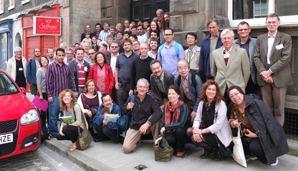
9 ÈÖ Ì ÛÓÖ ÓÔ ³Ë Ò ÙÐ Ö Ø Ò ÓÑ ØÖÝ Ò ÔÔÐ Ø ÓÒ ÁÁÁ³ Û Ø Ø Ö Ò ÕÙ Ò Ó ÒÒ Ð ÛÓÖ ÓÔ Ø Ö Ø Ò Ø Î Ð Ò ËÔ Ò Ò ¾¼¼ ½ Ò Ø ÓÒ Ø Ð ÛÓ ÈÓÐ Ò Ò ¾¼½½ ¾ º Ì Û ÓÐ ÕÙ Ò ØÖ ÙØ ØÓ Ø Ò Ô Ö Ø ÓÒ Ð ÛÓÖ Ó ÖÑ Ò ÊÓÑ ÖÓ Ù Ø Ö Ò Ø ÓÙÖØ Ø ÖÑ Ó Ø ÕÙ Ò ÙÐ ØÓ Ø ÔÐ Ò Â Ô Ò Ò ¾¼½ º Ì Ø Ö ÛÓÖ ÓÔ Ð Ø Ø ÁÒØ ÖÒ Ø ÓÒ Ð ÒØÖ ÓÖ Å Ø Ñ Ø Ð Ë Ò Á Å˵ Ò Ò ÙÖ ËÓØÐ Ò ÖÓÑ ¾ ØÓ Ë ÔØ Ñ Ö ¾¼½ ØØÖ Ø Ô ÖØ Ô ÒØ ÖÓÑ ½ ÓÙÒØÖ º Ì ÛÓÖ ÓÔ Ð Ö Ø Ø ¼ th ÖØ Ý Ó ËØ Ò Û Â Ò Þ Ó Ò ÒÐÙ Ð ØÙÖ ÓÙØ ÛÓÖ Ý ÏÓ ÓÑ ØÖÞº Ì ÔÐ Ò ÖÝ Ð ØÙÖ Û Ö ÓÐÐÓÛ Ò Ö Û Ù ÈÐ ÓÑÔÐ Ø ØÖ Ò Ú Ö Ð Ö Ú Ø ³ ÏÓÐ Ò Ð Ò Î Ö Ò Ó Ø ÜÔÓÒ ÒØ Ó ÓÖ ÓÐ Ä Ò Ù¹ ÒÞ ÙÖ ÑÓ Ð ³ ÓÓ Á Û Ì D 4 ¹ØÖ Ð ØÝ Ò Ò ÙÐ Ö Ø Ó Ø Ò ÒØ ÙÖ ³ Ë ÝÙ ÁÞÙÑ Ý Ù Ø Ó ÛÓÖÐ Ø Ò ÒØ ¹ Ë ØØ Ö Ô ³ ËØ Ò Û Â Ò Þ Ó ÝÐ Ò ÓÑ Ò ØÓÖ Ð Ô Ö Ñ ØÖ Þ Ø ÓÒ Ó Ø ØÖ Ö Ð Ò ³ ÇÐ Ã ÖÔ Ò ÓÚ ÐÓ Ð Ö Ð Ø ÓÒ ÓÖ ØÓÖ Ò ÙÐ Ö Ø ³ ÏÓ ÃÙ ÖÞ ËØÖ Ø ¹ Ð Ö Ú ØÓÖ ÙÒ Ð ³ Ò ØÓÐÝ Ä Ó Ö Ð Ò Ú Ö Ø Ó Ø Û Ø ÔÐ Ò ÙÖÚ Ò ÙÐ Ö Ø ³ Ú ÅÓÒ ÇÔ Ò ÔÖÓ Ð Ñ Ò Ò ÙÐ Ö Ø Ó Ñ ÔÔ Ò ÖÓÑn Ô ØÓn+1 Ô ³ Ò Ö Æ Ñ Ø Ä ØØ Ó ÓÑÓÐÓ Ý ÓÖ ÙÔ Ö ÓÐ Ø Ò Æ ÛØÓÒ ÒÓÒ Ò Ö Ø Ò ÙÐ ¹ Ö Ø ³ ÂÙ Ò ÂÓ ÆÙ Ó¹ ÐÐ Ø ÖÓ ÓÒØ Ø ÔÖÓÔ ÖØ Ó ÙÖ Ò ¹ Ô Û Ø ÓÖ Ò ½ Ò Ù¹ Ð Ö Ø ³ È ØÖ ÈÓÔ Ù¹È ÑÔÙ Ì Ð ¹ Ù Ð Ð ØØ Ó ÔÐ Ò Ö Ò ³ ÒÒ ÈÖ ØÓÙ Ú Ø À Ö Ô Ò ÙÒ Ð ÓÒ ÃÐ Ò ÙÖ ³ Ê Ö Ê Ñ ÒÝ Ì ÓÑ ÔÓÐÝÒÓÑ Ð ØÖÙØÙÖ ÓÒ Ø ÒØ ³ Î Ð Ú Ë Ý ÇÒ Ø ØÓÔÓÐÓ Ý Ó Ø Ð Ä Ö Ò Ñ ÔÔ Ò Û Ø Ò ÙÐ Ö Ø Ó ØÝÔ A Ò D³ Ë Ö Ý Ë Ö Ò ÓÖÖ ÔÓÒ Ò ØÛ Ò ÀÙÖÛ ØÞ ÒÙÑ Ö Ò ÑÓ ÙÐ Ó ÙÖÚ ³ Ò Ö ËÞ Ò Ì ÓÑ ÔÓÐÝÒÓÑ Ð Ò ÐÓ Ð Þ Ø ÓÒ³ Ö Ì Ö ÙÖÚ Ò ÙÖ Ò Ø Å Ò ÓÛ Ô ³ ÁÒ Ø ÓÒ ÓÒ Ð Ç³Ë Ð Ú Ö ÈÙ Ð Ä ØÙÖ ÓÒ Ø Ù Ø Ì ÄÙÖ Ó Ë Ò ÙÐ Ö ØÝ Ì ÓÖݳº ËÐ ÖÓÑ ÓÑ Ó Ø ÔÐ Ò ÖÝ Ò ÓØ Ö Ð ØÙÖ Ö Ú Ð Ð ÓÒ Ø ÛÓÖ ÓÔ³ Û Ô ØØÔ»»ÛÛÛº Ñ ºÓÖ ºÙ»ÛÓÖ ÓÔºÔ Ô ¾ ËÔ Ð Ø Ò Ö Ù ØÓ Ø Á ÅË ÓÖ Ø Ö Ü ÐÐ ÒØ ÓÖ Ò Þ Ø ÓÒº ÁÒ Ô ÖØ ÙÐ Ö Û Ø Ò Ø ÒØÖ Å Ò Ö Â Ò Ï Ð Ö Ò À Ð Ò Ö Ð Ò Û Ó Û Ø ÓÒ Ö Ò ÓÓÖ Ò ØÓÖ Ø Ø Ø Ø Ñ º Ï Ð Ó Ö Ø ÙÐÐÝ ÒÓÛÐ Ò Ò Ð ÙÔÔÓÖØ ÓÖ Ø ÛÓÖ ÓÔ ÖÓÑ Ø Á ÅË Ú Ø Ò Ò Ö Ò Ò È Ý Ð Ë Ò Ê Ö ÓÙÒ Ðµ Ø ÄÓÒ ÓÒ Å Ø Ñ Ø Ð ½ ÈÖÓ Ò Ó Ø Ö Ø ÏÓÖ ÓÔ ÓÒ Ë Ò ÙÐ Ö Ø Ò Ò Ö ÓÑ ØÖÝ Ò ÔÔÐ Ø ÓÒ ÌÓÔÓÐÓ Ý Ò Ø ÔÔÐ Ø ÓÒ ½ Ù ¾ ¾¼½¾º ¾ ÈÖÓ Ò Ó Ø Ë ÓÒ ÏÓÖ ÓÔ ÓÒ Ë Ò ÙÐ Ö Ø Ò ÓÑ ØÖÝ Ò ÔÔÐ Ø ÓÒ ÂÓÙÖÒ Ð Ó Ë Ò Ù¹ Ð Ö Ø ÎÓÐÙÑ ¾¼½¾º

10 ËÓ ØÝ Ò ÓÖ Ø Ö ÝÓÙÒ Ö Ö Ö ÖÓÑ Ø Íù ÁÒ Ø ØÙØ Ó Å Ø Ñ Ø Ò Ø ÔÔÐ Ø ÓÒ º Ø Ò Ó Ø Ô Ö Ú ÒÓÛ ÔÖ ÒØ Ø Ö ÛÓÖ Ò ÛÖ ØØ Ò ÓÖÑ Ö Ö ÖØ Ð ÙÖÚ Ý ÓÖ ÜÔÓ Ø ÓÒº Ï Ö Ö Ø ÙÐ ØÓ Ø Ô ÖØ Ô ÒØ ÓÖ Ø Ö Ø Ò Ò Ø Ö Ö Ò ÔÖÓ Ò ØÓ Ø ØÓÖ Ó Ø ÂÓÙÖÒ Ð Ó Ë Ò ÙÐ Ö Ø ÓÖ Ñ Ò ÔÓ Ð Ø Ô Ð Ù ÓÒØ Ò Ò ÓÑ Ó Ø Ø Ò Ð ÓÙØÓÑ Ó Ø ÛÓÖ ÓÔ Ò Ò ÙÖ º Â Ò¹È ÙÐ Ö Ð Ø È Ø Ö Ð Ò Î ØÓÖ ÓÖÝÙÒÓÚ Â ÒÙ ÖÝ ¾¼½

11 Ä Ø Ó È ÖØ Ô ÒØ Ð Ö Û Þ ÐÓÒ Ó¹ ÓÒÞ Ð Þ Ð Ñ ÒØ Ð ËÙÐ Ñ Ò Ö Ó ÂÓ Ñ ÐÓ Ø Ø Ö Ò ÌÙÖ Æ Ö ÓÖÓ Þ Å Ö Ð Ø Â Ò¹È ÙÐ ÖÙ ÐÐ Ò Ä Ò ÐÐ Ò ÛÓÖØ Ú Ö Ø Ò Ò Ë Ö Ò Ì Ò ÓÑ ØÖÞ ÏÓ ÓÒ Ð Ò È Ø Ö Ù ÈÐ Ò Ö Û Ð Ò ÏÓÐ Ò ÖÖ Ö Ó Ø ÂÓÓ ÖÐÓ Ð Ò È Ø Ö ÓÖÝÙÒÓÚ Î ØÓÖ Ö Ò Ò Î Ò ÒØ À Ð Ý ÂÓ Ð À ÖÒ Ò Å Ö ÐÓ Á Û ÓÓ ÁÞÙÑ Ý Ë Ù Â Ò Þ Ó ËØ Ò Û Ã ÖÔ Ò ÓÚ ÇÐ ÃÓÒ Ä Ò Ð Ò ÃÙ ÖÞ ÏÓ ÃÙ Ò Ö Ä ÓÒ Ä Ó Ö Ò ØÓÐÝ Ä ÒÒ Å Ð ÄÙ Û ÍÖ ÙÐ Å Ó ÒÓÖ Å ÒÓ Ð Å Ö Ñ Å Ö Ö ÌÓÒ Å ÖØ Ò ÖÒ Å ÖØ Ò ÊÓ Ö Ó Å Ò Â Ù Ø Ö Ò Å ÞÓØ Ù Ù ÅÓÒ Ú ÅÓÝ È Ö Þ ÂÙ Ò ÒØÓÒ Ó Æ Ñ Ø Ò Ö Æ ÑÙÖ Ì ÆÙ Ó¹ ÐÐ Ø ÖÓ ÂÙ Ò ÂÓ Ç³Ë ÓÒ Ð Ç ÙÑ ÌÓÑÓ ÖÓ Ç Ø Ë Ò Ê Ð È ÓÒ È ÓÖØ Ù ÐÐ ÖÑÓ ÈÓÔ Ù¹È ÑÔÙ È ØÖ ÈÖ ØÓÙ Ú Ø ÒÒ Ê Ò Ò Ö Û Ê Ú Ö Ñ Ê Ð Ý À Ø Ö Ê Ñ ÒÝ Ê Ö ÊÓÞ Ò Å Ö Ó ÊÓ Ö Ù À ÖÒ Ò Å Ö Ð Ò ÊÓÑ ÖÓ Ù Ø Ö Å Ö ÖÑ Ò Ë Å Ö ÐÓ Ë Ò Ö Ó Ð Ø Ö Ë Ö ÁÒÒ Ë Ý Î Ð Ú Ë Ö Ò Ë Ö Ý Ë Ö Ñ Ö Ë ÙÖ ÓÒ Ð ÙÖ ËØ Ú Ò Â Ò ËÞ Ò Ò Ö Ì Å ØÓÑÓ Ì Ö Ö ÌÓÑ ÖÙ Ì ÍÖ ¹Î Ö Ê Ö Ó Ï ÐÐ Ì ÖÖÝ Ï Ò Ò Ï Ö Ò ÖÞ Ï Ð Ö Å ÖØ Ò Ð Ù Ø Å Ø Ð Ù ÙÒÓ Ï Ø ÖÙ

12

13 Journal of Singularities Volume 12 (2015), 1-18 Proc. of Singularities in Geometry and Appl. III, Edinburgh, Scotland, 2013 DOI: /jsing a QUASI CUSP SINGULARITIES FAWAZ ALHARBI Abstract. We obtain a list of all simple classes of singularities of function germs with respect to the quasi cusp equivalence relation. We discuss its connection with the singularities of Lagrangian projections in presence of a cuspidal edge. We also describe the bifurcation diagrams and caustics of simple quasi cusp singularities. 1. Introduction In 2007, motivated by the needs of the theory of Lagrangian maps of singular varieties, Vladimir Zakalyukin classified function germs with respect to new non-standard equivalence relations (see [5, 6]) which he named quasi equivalences. The relations are aimed to control positions of only critical points of functions or maps and allow absolute freedom outside the critical locus. Zakalyukin s quasi equivalences are a very natural and efficient tool for classification of Lagrangian maps of smooth manifolds containing distinguished singular hypersurfaces which are playing the role of boundaries or of initial conditions in the corresponding system of differential equations. For comparison, Arnold s classical approach to classification of boundary functions singularities and, in general, of functions in presence of possibly singular hypersurfaces [3] corresponds to consideration of a pair of Lagrangian submanifolds meeting along a codimension 1 intersection. Zakalyukin s method allows to keep information only about one of the submanifolds of a pair and of the intersection set. Thus, the quasi equivalences of functions are considerably rougher than equivalences of functions on manifolds with (singular) boundaries. The quasi classifications of function singularities corresponding to smooth Lagrangian submanifolds with the boundary hypersurface being either smooth or a union of two smooth components meeting transversally have been considered in [6, 2]. In the present paper we study the case of the boundaries which are cylinders over generalized cuspidal curves x s 1 = x 2 2. The paper is organized as follows. In Section 2 we introduce our main notions, of the pseudo and quasi border equivalence relations, and derive an expression for the tangent space to the quasi cusp equivalence class of a function. In Section 3 we obtain the classifications of simple quasi cusp singularities. In Section 4, the bifurcation diagrams and caustics of simple quasi cusp singularities are described. Finally, in Section 5 we discuss the singularities of Lagrangian projections in presence of a cuspidal edge. Acknowledgements. I am deeply grateful to Vladimir Zakalyukin who introduced me to the idea of quasi border equivalence relation. I am also thankful to the anonymous referee and Victor Goryunov for their highly useful comments on the initial version of the paper. I gratefully acknowledge the support and generosity of the Umm Al-Qura University Mathematics Subject Classification. 58K05, 58K40, 53A15. Key words and phrases. Quasi border singularities, cusp, bifurcation diagram, caustic, Lagrangian projection.

14 2 FAWAZ ALHARBI 2. Pseudo and quasi border equivalence relations Consider a coordinate space R n with a hypersurface Γ in it. The hypersurface will usually be a cylinder, and we therefore split the coordinates on R n into y = (y 1, y 2,..., y n m ) which accommodate cylindrical directions for Γ and x = (x 1, x 2,..., x m ) in which an equation B(x) = 0 of Γ is written. When this distinction between x and y is not crucial, we will be using the notation w = (x, y) for the whole set of coordinates on R n. In the current paper, we consider the following shapes of Γ. 1. The hypersurface is smooth, in which case we set Γ = Γ b = {x 1 = 0}. 2. The hypersurface is a cylinder over a cusp: Γ = Γ csp = {x 2 2 x s 1 = 0 : s 3}. Remark 2.1. Notice that if s = 2 then the hypersurface {x 2 2 x 2 1 = 0} is diffeomorphic to the corner {x 1 x 2 = 0} which was discussed in [2]. We consider germs of C functions f : (R n, 0) R, in local coordinates w as above. We denote by C w the ring of all such germs at the origin. Definition 2.2. Two functions f 0, f 1 : R n R are called pseudo border equivalent if there exists a diffeomorphisim θ : R n R n such that f 1 θ = f 0, and if a critical point c of the function f 0 belongs to the border Γ then θ(c) also belongs to Γ and vice versa, if c is a critical point of f 1 and belongs to Γ then θ 1 (c) also belongs to Γ. A similar definition can be introduced for germs of functions. Remarks The general statements below are valid for reasonably good hypersurfaces. For rigorousness, we assume that the hypersurface Γ is a stratified set, and the stratification satisfies the Whitney condition A. Also, we assume in the definition 2.2 that if a critical point c belongs to some stratum of Γ then θ(c) belongs to the same stratum. 2. The pseudo border equivalence will be also called pseudo boundary or pseudo cusp for respective type of Γ. 3. The pseudo border equivalence is an equivalence relation: if f 1 f 2 and f 2 f 3 then f 1 f 3. However, this relation is not a group action as the set of admissible diffeomorphisms depends on a function. Definition 2.4. Let J be an ideal in C w, then we define the radical Rad(J) of the ideal J as the set of all elements in C w, vanishing on the set of common zeros of germs from J: Rad(J) = I(V (J)), where and V (J) = {w R n : h(w) = 0 for all h J}, I(V (J)) = {ϕ C w : ϕ(w) = 0 for all w V (J)}. A similar definition can be introduced when we replace C w by the space R[w] of all real polynomials in the variables w. In general, the radical of an ideal behaves badly when the ideal depends on a parameter.

15 QUASI CUSP SINGULARITIES 3 Example 2.5. Consider the family of ideals J ε = w(w ε)r[w], w R, depending on ε R. Then, { J Rad(J ε ) = ε if ε 0 wr[w] if ε = 0. Hence, the dimension of the quotient space R[w]/Rad(J ε ) varies with ε: { 2 if ε 0 dim [R[w]/Rad(J ε )] = 1 if ε = 0. Recall that a vector field v preserves a hypersurface Γ = {B(x) = 0} if the Lie derivative L v B belongs to the principal ideal generated by B. The module S Γ of all germs of C vector fields preserving a hypersurface germ (Γ, 0) (R n, 0) is the Lie algebra of the group of diffeomorphims of (R n, 0) preserving (Γ, 0). The module S Γ is called the stationary algebra of (Γ, 0). Thus: If the border is smooth Γ b = {x 1 = 0}, then { S Γb = x 1 h n 1 + k i, x 1 y i i=1 h, k i C w Here x = x 1 R and y = (y 1, y 2,..., y n 1 ) R n 1. If the border is a cuspidal edge Γ csp = {x 2 2 x s 1 = 0 : s 3}, then { } S Γcsp = ( x 1 s h 1 + 2x 2 h 2 ) + ( x 2 x 1 2 h 1 + sx1 s 1 h 2 ) n 2 + k i, h 1, h 2, k i C w. x 2 y i i=1 Here x = (x 1, x 2 ) R 2 and y = (y 1, y 2,..., y n 2 ) R n 2. Suppose that all function germs in a smooth family f t are pseudo border equivalent to the function germ f 0, f t θ t = f 0, t [0, 1], with respect to a smooth family θ t : (R n, 0) (R n, 0) of germs of diffeomorphisms such that θ 0 = id and t [0, 1]. Denote by Rad{I t } the radical of the gradient ideal I t of the function f t. Then we have the homological equation: where the vector field f m t t = n m f t f t Ẋ i (t) + Ẏ j (t), x i=1 i y j=1 j v t = m i=1 Ẋ i (t) n m + Ẏ j (t) x i y j generates the phase flow θ t and its components satisfy the following: If the border is smooth then j=1 Ẋ 1 (t) {x 1 h + Rad{I t }} and Ẏ i (t), h C w, for all i. [6] If the border is a cuspidal edge then { x1 } Ẋ 1 (t) s h 1 + 2x 2 h 2 + Rad{I t }, Ẋ 2 (t) }. { x2 } 2 h 1 + sx s 1 1 h 2 + Rad{I t } and Ẏi(t), h 1, h 2 C w, for all i. We modify the pseudo equivalence relation to have a better parameter dependence. Namely, we replace Rad{I t } by the ideal I t itself in the equivalence definition.

16 4 FAWAZ ALHARBI Definition 2.6. Two functions f 0, f 1 : R n R are called quasi border equivalent, if they are pseudo border equivalent and there is a family of functions f t which depends continuously on parameter t [0, 1] and a continuous piece-wise smooth family of diffeomorphisms θ t : R n R n also depending on t [0, 1] such that: f t θ t = f 0, θ 0 = id and the components of the vector field v t generating θ t on each segment of smoothness satisfy the following: If the border is smooth, then Ẋ 1 (t) {x 1 h + I t } and Ẏ i (t), h C w, for all i. [6] If the border is a cuspidal edge, then Ẋ 1 (t) { x1 s h 1 + 2x 2 h 2 + I t }, Ẋ 2 (t) and Ẏi(t), h 1, h 2 C w, for all i. { x2 2 h 1 + sx s 1 1 h 2 + I t } Remarks Such a family θ t of diffeomorphisms generated by the vector field v t as well as the vector field itself will be called admissible for the family f t. 2. The tangent space T QΓ f to the quasi border equivalence class of f has the following description: If the border is smooth, then { f T QΓ f := T QB f = x 1 ( x 1 h + f x 1 A If the border is a cuspidal edge, then { f T QΓ f := T QCU f = x 1 + f x 2 + n 2 i=1 ( x1 ) n 1 f + k i, y i i=1 h, A, k i C w s h 1 + 2x 2 h 2 + f x 1 A 1 + f x 2 A 2 ( x2 2 h 1 + sx s 1 1 h 2 + f x 1 B 1 + f f y i C i, h 1, h 2, A i, B i, C i C w ) B 2 x 2 } ) }. Due to the inclusion I 2 0 T QΓ f I 0, where I 0 is the gradient ideal of f, we have Proposition 2.8. For any border, a function germ f has a finite codimension with respect to the quasi border equivalence if and only if f has a finite codimension with respect to the right equivalence. Definition 2.9. Two function germs are said to be stably quasi border equivalent if they become quasi border equivalent after the addition of non-degenerate quadratic forms in an appropriate number of extra cylindrical variables. Following [4], we call a function germ simple if its sufficiently small neighbourhood in the space of all function germs contains only a finite number of quasi equivalence classes. The quasi border classification of critical points outside the border Γ coincides with the standard right equivalence. Hence the standard classes A k, D k, E 6, E 7 and E 8 form the list of simple classes in this case. Also by definition, non-critical points are all equivalent wherever they are. Classification of critical points on a smooth border was done in [6]. So we classify in this paper only critical points on a cuspidal edge.

17 QUASI CUSP SINGULARITIES Basic techniques of the classification and prenormal forms. We will use Moser s homotopy method and the following technique which is similar to Lemma 8.1 [2] to establish quasi cusp equivalence between function germs. Let us fix a convenient Newton diagram Z n 0. The ideals S γ of function germs of the Newton order at least γ, γ 0, equip the ring C w with the Newton filtration: S 0 = C w, S δ S γ if δ < γ [4]. We assume here that the scaling factor for the orders is chosen so that functions with the Newton diagram have order N. Let f = f 0 + f be a decomposition of a function germ f into its principal part f 0 of the Newton degree N and higher order terms f. We assume that f 0 has a finite codimension with respect to the right equivalence. Lemma Consider a monomial basis of the linear space C w /T QCU f0. Let e 1 (w), e 2 (w),..., e s (w) be all its elements of Newton degrees higher than N. Suppose that for any ϕ S γ \ S >γ, γ > N: 1. There is an admissible vector field ẇ = ẇ i w i ẋ 1 = x 1 s h 1 + 2x 2 h 2 + where ẇ = (ẋ 1, ẋ 2, ẏ 1, ẏ 2,..., ẏ n 2 ), n i=1 A 1,i f 0 w i, ẋ 2 = x 2 2 h 1 + sx s 1 1 h 2 + and ẏ 1,..., ẏ n 2 C w, with h 1, h 2, A 1,i, A 2,i C w, such that ϕ = n i=1 f 0 w i ẇ i + ϕ + s c i e i (w), where ϕ S >γ and c i R. 2. Moreover, for any δ, N < δ < γ, and any ψ S δ the expression 2 ψ n ψ 2 E(ψ, ϕ) = ẋ i + A i,j f 0 n + 2 ψ A i,j + x i w j x i w j belongs to S γ. i=1 j=1 i=1 i=1 j=1 n i=1 A 2,i f 0 w i, n 2 i=1 ψ y i ẏ i Then any germ f = f 0 + f is quasi cusp equivalent to a germ f 0 + s a i e i, where a i R. We do not prove the Lemma here. The actual proof goes along the lines of Sections of [4] by induction on increasing γ. Condition 1 of the Lemma allows us to move degree γ terms of a function f to higher degrees modulo a degree γ linear combination of the e i. Condition 2 guarantees that the error term produced at such a move by the already normalised part (of degrees below γ) of the function does not affect this part. Remark A version of the Lemma is also valid for functions with the Newton principal part f 0 of infinite right equivalence codimension, which is the same as having dim (C w /T QCU f0 ) =. Namely, still assuming the Newton degree of f 0 being N, let e 1 (w),..., e s (w) be the degrees higher than N part of a monomial basis of C w / (T QCU f0 + S M ) for some M > N. Assume i=1

18 6 FAWAZ ALHARBI the conditions of Lemma 2.10 hold for all γ < M. Then, using the ideas hinted for the proof of the Lemma, one can show that any function with the Newton principal part f 0 is quasi cusp equivalent to s f 0 + a i e i + Ψ, where Ψ S M. i=1 If M may be taken arbitrary here, this means in practice that, when classifying functions of finite quasi cusp codimension, we may consider functions with the principal part f 0 being reduced to the form f 0 + s a i e i where this time the sum is infinite: the e i are the degrees higher than N i=1 part of a monomial basis of a transversal to the quasi cusp orbit of f 0 in the ring of formal power series in w, and a i R. Lemma 2.10 and the above remark are essential for our normal form reduction in Section 3. It helps us in situations not covered by the technique of chapter 12 of [4], for example when f 0 is quasihomogeneous with respect to certain weights of the variables in which basic fields tangent to the border are not quasihomogeneous Quadratic terms. Now, let f : (R n, 0) (R, 0) be a function germ of the form f(x, y) = f 2 (x, y) + f 3 (x, y), where f 2 is a quadratic form in x and y, and f 3 M 3 x,y. Lemma Let f : (R 2, 0) (R, 0) be a function germ at the origin in local coordinates x 1 and x 2 only. If f 2 is a non-degenerate quadratic form then f is quasi cusp equivalent to ±x 2 1±x 2 2. Proof. In this case vector fields with components from the gradient ideal of a function with a non-degenerate quadratic part are all vector fields vanishing at the origin. Therefore any family of diffeomorphisms preserving the origin is admissible, and the Lemma follows from the standard Morse Lemma. Let n 2 and set f (y) = f x=0. Denote by r the rank of the second differential d 2 0f at the origin. Set c = n 2 r. Denote by r the rank of the second differential d 2 0f at the origin. Lemma (Stabilization) The function germ f(x, y) is quasi cusp equivalent to a germ r i=1 ±yi 2 + g(x, ỹ), where ỹ Rc and g M 3 ỹ. For quasi cusp equivalent germs f, the respective reduced germs g are quasi cusp equivalent. Proof. Up to a linear transformation in y, we have r n 2 2 f = ±yi 2 + a i,j y i x j + Q 2 (x) + f 3 (x, y), (1) i=1 i=1 j=1 with f 3 M 3 x,y and Q 2 a quadratic form in x only. Let ŷ = (y 1, y 2,..., y r ) and ỹ = (y r +1,..., y n 2 ) R n 2 r. Then, (1) can be written as f 1 = r i=1 ±y 2 i + ϕ(x, ŷ, ỹ) + f(x, ỹ),

19 QUASI CUSP SINGULARITIES 7 where and ϕ = r 2 a i,j y i x j + r i=1 j=1 l=1 y l ϕ l (x, y) with ϕ l M 2 x,y, f = Q 2 (x) + We now aim to find a family n 2 i=r +1 j=1 of diffeomorphisms which eliminates ϕ. 2 a i,j y i x j + f 3 (x, ỹ) with f3 M 3 x,ỹ. θ t : (x, y) ( x, Ŷt(x, ŷ), ỹ ) Take a family f t = r i=1 ±y2 i +tϕ(x, ŷ, ỹ)+ f t (x, ỹ) which joins f 1 and f 0 = r i=1 ±y2 i + f 0 (x, ỹ) with t [0, 1] and f = f 1. Here, f t and f 0 are unknown. So, we want to solve the homological equation for ẏ and simultaneously for f t. The homological equation takes the form f 2 t t = f t ẋ i + x i i=1 r i=1 f t y i ẏ i + n 2 j=r +1 f t y j ẏ j. (2) Note that ẋ 1 = ẋ 2 = y j = 0, j = r + 1,..., n 2, as x and ỹ do not change with t. Thus, equation (2) can be written as (ϕ + f r t t ) = (±2y i + t ϕ )ẏ i. (3) y i i=1 Set z i = ±2y i + t ϕ y i, i = 1,..., r, which are known functions. Note that the matrix ( zi ŷ j ) has the maximal rank at the origin for any value of t. Hence we can take z = (z 1, z 2,..., z r ) as new coordinates instead of ŷ. Thus, equation (3) takes the form (ϕ + f r t t ) = z i ẏ i Using the Hadamard Lemma, we write this as r i=1 By taking ψ i = ẏ i and f t t i=1 z i ψ i (x, z, ỹ, t) + φ(x, ỹ, t) + f r t t = z i ẏ i. i=1 = φ, we show that the homological equation is solvable. The last step is to find f 0. This can be done using the relation 1 Note that the vector field v = r 0 φdt = ẏ i i=1 1 0 f t t dt = f 1 f 0. y i is defined in some neighborhood of the segment [0, 1] of the t-axis in the space R n R t, which is due to the z i vanishing on this segment.

20 8 FAWAZ ALHARBI Hence all the f t are quasi cusp equivalent. In particular, the function germ f 1 is quasi cusp equivalent to f 0. The second claim of the Lemma can be deduced directly as the family ( ) θ t : (x, y) x, Ŷt(x, ŷ), ỹ preserves the projection (x, ŷ, ỹ) (x, ỹ). Lemma Let f : (R n, 0) R be a function germ with an isolated critical point at the origin, and I 0 its gradient ideal. Then f is quasi cusp equivalent for each t [0, 1] to the function germ g t (w) = f(w) + th(w) with h(w) I 2 0, provided that the rank r of the second differential d 2 0g t of g t at the origin is constant. Proof. At first we claim that if the rank of d 2 0g t is constant then for different t the gradient ideals I t of g t coincide. Since the claim does not depend on the choice of local coordinates, we may assume that the quadratic part of f at the origin has diagonal form r ε i wi 2, where ε i = ±1 for i = 1,..., r. We also set ε i = 0 for i > r. The quadratic part of g t at the origin is r ( εi δ ij wi 2 ) r + 4th ij (0)ε i ε j w i w j = D ij w i w j i,j=1 i,j=1 where the h ij, i, j = 1,..., n are the coefficients of the decomposition n h(w) = h ij (w) f f w i w j i,j=1 of the function h, δ ij is the Kronecker symbol, and D ij = ε i δ ij + 4tε i ε j h ij (0). We will assume here that h ij = h ji. The r r matrix with entries D ij is invertible for any t since the rank of d 2 0g t is r. Reversing signs of some of its rows, we see that the n n matrix with the entries ˆD ij = δ ij + 4tε j h ij (0), for i, j = 1,..., r and ˆD ij = δ ij otherwise, is also invertible. The differentiation g t w i = f w i + t n k,j=1 ( 2h kj implies that I t I 0. This derivative can also be written as g t w i = n j=1 (δ ij + 4tε i h ij (0) + R ji ) f w j = i=1 2 f + h ) kj f f w k w i w i w k w j n j=1 ( ˆDji + R ji ) f w j, where the functions ( R ij vanish ) at w = 0. So in some neighborhood of the interval [0, 1] of the t-axis the matrix ˆDji + R ji is invertible. This implies that I 0 I t. Hence, I t = I 0. Now the homological equation gt t = n i=1 g t w i V i can be solved for the unknown functions V i which belong to the gradient ideal I t for any t, since the left hand side belongs to the square of this ideal. The phase flow of the vector field V i w i leaves all critical points of g t fixed. Hence all the germs g t are quasi cusp equivalent.

21 QUASI CUSP SINGULARITIES 9 Lemmas 2.13 and 2.14 imply the following improved stabilization splitting. Lemma There is a non-negative integer s r r such that the function germ f(x, y) is quasi cusp equivalent to r +s ±yi 2 + f(x, ỹ), where ỹ R c s and f is a sum of a function germ i=1 from M 3 x,ỹ and a quadratic form in x only. For quasi cusp equivalent germs f, the corresponding reduced germs f are quasi cusp equivalent. Proof. Due to Lemma 2.13, we can assume that the quadratic part of the function is f 2 = r ±yi 2 + x n 2 n 2 1 α 1,i y i + x 2 α 2,i y i + g 2 (x) with constant coefficients α j,i and the i=1 i=r +1 i=r +1 quadratic form g 2 in x only. Suppose that some of these coefficients, for example α 1,r +1, is ( ) 2 non-zero. Then, summing up the function f with δ f x 1 for sufficiently small δ gives a new function g which (according to Lemma 2.14) is quasi cusp equivalent to f and contains the term yr 2 +1 with a non-zero coefficient. Therefore the rank of the restriction of g to the x = 0 subspace is larger than r. Repeating the procedure several times, if needed, we get a function germ with a larger value of r and without the x j y >r terms. This is exactly the form required. 3. Classification of simple functions We start this section with recalling the classification of simple singularities with respect to the quasi boundary equivalence relation from [6]. After that we classify simple quasi cusp singularities, giving details of proofs of main results Simple quasi boundary classes. Classifications of simple quasi boundary singularities is as follows. Theorem 3.1. [6] On the boundary x 1 = 0, any simple quasi boundary singularity class is a class of stabilizations of one of the following two-variable germs: Notation Normal form Restrictions codimension B k ±y1 2 ± x k 1 k 2 k F k,m ±(x 1 ± y1 k ) 2 ± y1 m 2 k < m k + m 1 Remarks Any germ f with the quadratic part of corank greater than 1 is non-simple. 2. The only fencing singularity is the uni-modal class S 5 : y1 3 + x ax 2 1y 1, a R \ { }, which is adjacent to F 2,3. 3. Any corank 1 germ is either simple (and hence quasi boundary equivalent to one of the germs in the above theorem) or belongs to a subset of infinite codimension in the space of all germs. 4. The graph of low codimension adjacencies is as follows: B 2 B 3 B 4 B 5 B 6... F 2,3 F 2,4 F 2,5 F 2,6... S 5 F 3,4 F 3,5 F 3,

22 10 FAWAZ ALHARBI 3.2. Simple quasi cusp classes. We distinguish the following cases: 1. If the base point of a function germ is at a regular point of the border: Γ csp = {x 2 2 x s 1 = 0 : s 3}, then the quasi cusp equivalence coincides with the quasi boundary equivalence. Hence, the list of simple quasi cusp classes in this case is the same as that of simple quasi boundary classes. 2. The remaining case of a function germ having a critical base point on the cusp stratum is described by the following theorem. Theorem 3.3. Let a function germ f : (R n, 0) (R, 0), be simple with respect to the quasi cusp equivalence. Then, either its quadratic part f 2 is non-degenerate and hence f is quasi cusp equivalent to L 2 : ±x 2 1 ± x n 2 ±yi 2 or f 2 has corank 1 in which case f is stably quasi i=1 cusp equivalent to one of the following simple classes: Notation Normal form Restrictions Codimension L k ±x 2 1 ± x k 2 k 3 k + 1 M k ±x 2 2 ± x k 1 s = 3, k 3 k + 2 M 3 ±x x 3 1 s 4 5 N 2,2,k ±(x 1 + y1) 2 2 ± (x 2 + y1) 2 2 ± y1 k s = 3, k 3 k + 3 N 2,2,3 ±(x 1 + y1) 2 2 ± (x 2 + y1) y1 3 s 4 6 N 2,3,4 ±(x 1 + y1) 2 2 ± (x 2 + y1) 3 2 ± y1 4 s = 3 8 N 3,3,4 ±(x 1 + y1) 3 2 ± (x 2 + y1) 3 2 ± y1 4 s = 3 9 Remarks Any germ f with the quadratic part of corank greater than 1 is non-simple. 2. Any germ of corank 1 is either simple (and hence quasi cusp equivalent to one of the germs in the above theorem) or belongs to a subset of infinite codimension in the space of all germs. 3. The fencing classes are stabilizations of the following: Notation Class Restrictions Codimension L ±x βx 1 x γx 3 2 β, γ R, 4β 3 ± 27γ M 4 ±(x 2 + δx 2 1) 2 ± x 4 1 s 4, δ R 6 N 2,3,5 ±(x 1 + y1) 2 2 ± (x 2 + y1) αy1 5 s = 3, α R \ {0} 9 4. The graph of adjacencies in low codimension (when s = 3) is as follows: Also, M 3 L. L 2 L 3 L 4 L 5 L 6... M 3 M 4 M 5 M 6... N 2,2,3 N 2,2,4 N 2,2,5 N 2,2,6... N 2,3,4 N 2,3,5 N 3,3,4 To prove Theorem 3.3, we need the following auxiliary results.

23 QUASI CUSP SINGULARITIES 11 Lemma 3.5. Let κ = n r be the corank of the second differential d 2 0f at the origin. 1. If κ = 0, then f is quasi cusp equivalent to n 2 ±yi 2 + f 2(x 1, x 2 ) + f 3 (x 1, x 2 ), where f 2 is a non-degenerate quadratic form and f 3 M 3 x 1,x 2. n 2 2. If κ = 1, then f is quasi cusp equivalent to either ±yi 2 + f(x 1, x 2 ) with ( rank d 2 f ) n 2 0 = 1 or to ±yi 2 ± x 2 1 ± x f 3 (x 1, x 2, y 1 ) where f 3 (x 1, x 2, y 1 ) M 3 x 1,x 2,y 1. i=2 3. If κ 2, then f is non-simple. Proof. Lemmas 2.12 and 2.15 provide the first two parts of Lemma 3.5. For part 3, suppose that κ = 2. Then Lemma 2.15 yields that any function germ f(x 1, x 2, y) reduced to one of the following forms: n 2 0. F 0 = ±yi 2 + f 3 where f 3 M 3 x 1,x 2, or i=1 n 2 1. F 1 = ±yi 2 + f 2 (x 1, x 2 ) + f 3 where f 3 M 3 x 1,x 2,ỹ 1, ỹ 1 R and f 2 is a quadratic form of i=2 rank one, or n 2 2. F 2 = ±yi 2 + f 2 (x 1, x 2 ) + f 3 where f 3 M 3 x, ỹ = (ỹ 1,x 2,ỹ 1, ỹ 2 ) and f 2 is a non-degenerate i=3 quadratic form. Consider the germ F 0. The tangent space to the quasi cusp orbit at the germ f 3 is T QCU f3 = f { 3 x1 x 1 s h 1 + 2x 2 h 2 + f 3 A 1 + f } 3 A 2 x 1 x 2 + f { 3 x2 x 2 2 h 1 + sx s 1 1 h 2 + f 3 B 1 + f } 3 B 2. x 1 x 2 The cubic terms in T QCU f3 are from ( x1 s ) f 3 h 1 x 2 i=1 i=1 ( f 3 2x 2 + sx1 s 1 x 1 ) h 2, f 3 + x 2 f 3 and x 1 2 x 2 where h 1, h 2 R. These terms form a subspace of dimension at most 2. The dimension of the space of all cubic forms in x 1 and x 2 is 4 which is greater than the subspace dimension. This means that the germ F 0 is non-simple. In the next case we have F 1 = n 2 i=2 ±y2 i ± (ax 1 + bx 2 ) 2 + f 3, where f 3 M x1,x 2,ỹ 1, and a, b R (a and b are not both zeros). Note that F 1 deforms to n 2 F 1 = ±yi 2 ± (ax 1 + bx 2 + δỹ 1 ) 2 + f 3, δ 0. i=2 According to Lemma 2.15, F 1 is quasi cusp equivalent to n 2 i=1 ±y2 i + f with f M 3 x 1,x 2, which we have already shown to be non-simple. Similar argument yields that F 2 is adjacent to F 1 and the result follows.

24 12 FAWAZ ALHARBI Lemma 3.6. Let f : (R 2, 0) (R, 0) be a function germ in local coordinates x 1 and x 2, and with a critical point at the origin. If the quadratic form f 2 of f has rank 1 then f is quasi cusp equivalent to either ±x ϕ 1 (x 2 ) where ϕ 1 M 3 x 2 or ±x ϕ 2 (x 1, x 2 ) where ϕ 2 M 3 x 1,x 2. Moreover, if s = 3 then ±x ϕ 2 (x 1, x 2 ) is quasi cusp equivalent to ±x ϕ 3 (x 1 ) where ϕ 3 M 3 x 1. Proof. We have f = ±(ax 1 + bx 2 ) 2 + f 3 (x 1, x 2 ), where f 3 M 3 x 1,x 2 and a, b R (a and b are not both zeros). Consider Q 1 = ±(ax 1 + bx 2 ) 2 and suppose that a 0. Take the homotopy Q t = ±(ax 1 + tbx 2 ) 2 where t [0, 1]. The corresponding homological equation is { x1 } ±2bx 2 (ax 1 + tbx 2 ) = ±2a(ax 1 + tbx 2 ) s h 1 + 2x 2 h 2 + (ax 1 + tbx 2 )A { x2 } ±2tb(ax 1 + tbx 2 ) 2 h 1 + sx1 s 1 h 2 + (ax 1 + tbx 2 )B. This is equivalent to { x1 } { bx 2 = a s h x2 } 1 + 2x 2 h 2 + (ax 1 + tbx 2 )A + tb 2 h 1 + sx s 1 1 h 2 + (ax 1 + tbx 2 )B. The homological equation is solvable by setting h 1 = B = 0 and taking constants A and h 2 such that a 2 A + tbsx1 s 2 h 2 = 0 and 2ah 2 + atba = b. These two equations in the variables A and h 2 are linearly independent. Thus, all the Q t, t [0, 1], are quasi cusp equivalent. In particular, Q 1 = ±(ax 1 +bx 2 ) 2 is quasi cusp equivalent to ±x 2 1. Now, consider the germ F = ±x f 3 (x 1, x 2 ), f 3 M 3 x 1,x 2. Let F 0 = ±x 2 1. The quasi cusp tangent space at F 0 is { x1 } T QCU F0 = ±2x 1 s h 1 + 2x 2 h 2 + x 1 A 1. Thus, we get mod T QCU F0 : x and x 1 x 2 0. Hence, C x1,x 2 /T QCU F0 C x2 + Rx 1. According to Remark 2.11, the germ F is quasi cusp equivalent to ±x ϕ 1 (x 2 ) with ϕ 1 M 3 x 2. If a = 0 and b 0 then f reduces to ±x ϕ 2 (x 1, x 2 ), ϕ 2 M 3 x 1,x 2. Suppose that s = 3. Consider the germ f 0 = ±x 2 2. Similar to the argument above, the germ f is quasi cusp equivalent to ±x ϕ 3 (x 1 ), where ϕ 3 M 3 x 1. Lemma 3.7. A function germ f(x 1, x 2, y 1 ) = ±x 2 1 ± x f 3 (x 1, x 2, y 1 ), f 3 M 3 x 1,x 2,y 1, is quasi cusp equivalent to f(x 1, x 2, y 1 ) = ±x 2 1 ± x x 1 φ 1 (y 1 ) + x 2 φ 2 (y 1 ) + φ 3 (y 1 ) where φ 1, φ 2 M 2 y 1 and φ 3 M 3 y 1. Proof. Consider the principal part f 0 = ±x 2 1 ± x 2 2. The quasi cusp tangent space to the orbit at f 0 is { x1 } { T QCU f0 = ±2x 1 s h x2 } 1 + 2x 2 h 2 + x 1 A 1 + x 2 A 2 ± 2x 2 2 h 1 + sx1 s 1 h 2 + x 1 B 1 + x 2 B 2. Thus, we get mod T QCU f0 : x 2 1 0, x and x 1 x 2 0. Hence, we have C x1,x 2,y 1 /T QCU f0 {x 1 ϕ 1 (y 1 ) + x 2 ϕ 2 (y 1 ) + ϕ 3 (y 1 ) : ϕ 1, ϕ 2, ϕ 3 C y1 }. Due to the constraint in the lemma on the term f 3, the claim of the lemma follows.

25 QUASI CUSP SINGULARITIES Proof of the main Theorem 3.3. Lemmas 3.5, 3.6 and 3.7 yield that all simple quasi cusp singularities are among the following germs: 1. G 1 = ±x ϕ 1 (x 2 ), where ϕ 1 M 3 x G 2 = ±x ϕ 2 (x 1, x 2 ), where ϕ 2 M 3 x 1,x G 3 = ±x 2 1 ± x x 1 φ 1 (y 1 ) + x 2 φ 2 (y 1 ) + φ 3 (y 1 ), where φ 1, φ 2 M 2 y 1 and φ 3 M 3 y 1. Using Lemma 2.10, one can easily prove the results below. Consider the germ G 1. Let ϕ 1 (x 2 ) = a k x k 2 + ϕ(x 2 ) where a k 0, k 3 and ϕ M k+1 x 2. Then, G 1 is quasi cusp equivalent to the germ L k : ±x 2 1 ± x k 2. Next, consider the germ G 2. Let s = 3. Then, by Lemma 3.6, G 2 is quasi cusp equivalent to G = ±x ϕ 3 (x 1 ), where ϕ 3 M 3 x 1. In this case G can be reduced to one of the functions M k : ±x 2 2 ± x k 1, k 3. Let s 4. If ϕ 2 contains a term ax 3 1, a 0, then G 2 is equivalent to M 3 : ±x x 3 1. Otherwise, in the most general case, G 2 is equivalent to a non-simple germ M 4 : ±(x 2 + δx 2 1) ± x 4 1, δ R. Finally, consider the germ G 3 : G 3 = ±x 2 1±x 2 2+x 1 (a 2 y 2 1 +a 3 y 3 1 +a 4 y )+x 2 (b 2 y 2 1 +b 3 y 3 1 +b 4 y )+c 3 y 3 1 +c 4 y 4 1 +c 5 y Suppose s = 3. If c 3 0, then G 3 is quasi cusp equivalent to ±x 2 1 ± x 2 2 equivalently as N 2,2,3 : ±(x 1 + y1) 2 2 ± (x 2 + y1) y y 3 1, which can be written If c 3 = 0, b 2 0 and c 4 ± b2 2 4, then G 3 is quasi cusp equivalent to ±x 2 1 ± x x 2 y 2 1 ± y 4 1, which is also quasi cusp equivalent to N 2,2,4 : ±(x 1 + y 2 1) 2 ± (x 2 + y 2 1) 2 ± y 4 1. If c 3 = 0, b 2 0 and c 4 = ± b2 2 4, then we get the classes N 2,2,k : ±(x 1 +y 2 1) 2 ±(x 2 +y 2 1) 2 ±y k 1, where k 5 (one may omit y 2 1 in the first bracket here). If c 3 = b 2 = 0, a 2 0 and c 4 ± a2 2 4, then G 3 is quasi cusp equivalent to ±x 2 1 ± x 2 2 ± x 1 y 2 1 ± y 4 1, which is equivalent to N 2,3,4 : ±(x 1 + y 2 1) 2 ± (x 2 + y 3 1) 2 ± y 4 1. If c 3 = a 2 = b 2 = 0, and c 4 0, then we get the class ±x 2 1 ± x 2 2 ± y 4 1 or, equivalently, the N 3,3,4 class: ±(x 1 + y 3 1) 2 ± (x 2 + y 3 1) 2 ± y 4 1. If c 3 = b 2 = 0, a 2 0 and c 4 = ± a2 2 4, then we get a non-simple class with α R \ {0}. N 2,3,5 : ±(x 1 + y 2 1) 2 ± (x 2 + y 3 1) 2 + αy 5 1 Now let s 4. Suppose c 3 0. Then, similar to the s = 3 case, the germ G 3 is quasi cusp equivalent to ±x 2 1 ± x 2 2 ± y 3 1, and hence to N 2,2,3 : ±(x 1 + y 2 1) 2 ± (x 2 + y 2 1) 2 + y 3 1. If c 3 = 0, then G 3 is adjacent to the non-simple germ M 4. This finishes the proof of the theorem.

26 14 FAWAZ ALHARBI 4. Bifurcation diagrams and caustics of simple quasi cusp singularities A quasi cusp miniversal deformation of a function germ f : (R n, 0) (R, 0) may be constructed in the standard way as τ 1 F (x, y, λ) = f(x, y) + λ i e i (x, y), (4) where e 0,..., e τ 1 C x,y project to a basis of C x,y /T QCU f. We will use the notation F λ for F λ=const, so that F 0 = f. Definition 4.1. The quasi cusp bifurcation diagram of a function germ f is the set of all points λ in the base R τ of its quasi cusp miniversal deformation for which either the set {F λ = 0} R n is singular, or a singularity of {F λ = 0} is on the border x 2 2 x s 1 = 0. Respectively, this diagram consists of two components, W 1 and W 2 : W 2 W 1, dimw j = τ j. Now assume that e 0 = 1 in (4), and all the other e i are from M x,y. Following the standard approach, we call the space R τ 1 of the parameter λ 1,..., λ τ 1 the base of a truncated quasi cusp miniversal deformation of f. Definition 4.2. Consider the projection map Π : R τ R τ 1 between the two bases, forgetting λ 0. The quasi cusp caustic of a function f is a hypersurface in the base R τ 1 which is a union of the Π-image Σ 1 of the cuspidal edge of the set W 1 R τ, and of the set Σ 2 = Π(W 2 ). Remark 4.3. In terms of Section 5 below, the component W 1 is the critical value set of the Lagrangian map of the manifold L, and W 2 is the image of the border Γ. All simple quasi cusp singularities are the A k singularities with respect to the standard right equivalence. So, the first component of the quasi cusp bifurcation diagram of a simple quasi cusp function is a product of a generalized swallowtail and R τ k. A similar observation is valid for the first components of the caustics. The versal deformations listed below provide an explicit description of the bifurcation diagrams and caustics of simple quasi cusp singularities. Proposition 4.4. Quasi cusp miniversal deformations of simple quasi cusp classes are as follows: Singularity Miniversal deformation Restrictions ±x 2 1 ± x k 2 + k 1 λ i x i 2 + λ k x 1 k 2 L k M k ±x 2 2 ± x k 1 + k 1 i=0 i=0 i=0 λ i x i 1 + λ k x 2 + λ k+1 x 1 x 2 s = 3, k 3 M 3 ±x x λ 0 + λ 1 x 1 + λ 2 x λ 3 x 2 + λ 4 x 1 x 2 s 4 ±(x 1 + y1) 2 2 ± (x 2 + y1) 2 2 ± y1 k + k 2 λ i y1 i s = 3, k 3 N 2,2,k +λ k 1 x 1 + λ k x 2 + λ k+1 x 1 y 1 + λ k+2 x 2 y 1 N 2,2,3 ±(x 1 + y1) 2 2 ± (x 2 + y1) y1 3 + λ 0 + λ 1 y 1 + λ 2 x 1 s 4 +λ 3 x 2 + λ 4 x 1 y 1 + λ 5 x 2 y 1 N 2,3,4 ±(x 1 + y1) 2 2 ± (x 2 + y1) 3 2 ± y1 4 + λ 0 + λ 1 x 1 + λ 2 x 2 s = 3 +λ 3 x 1 y 1 + λ 4 x 2 y 1 + λ 5 x 2 y1 2 + λ 6 y 1 + λ 7 y1 2 N 3,3,4 ±(x 1 + y1) 3 2 ± (x 2 + y1) 3 2 ± y1 4 + λ 0 + λ 1 x 1 + λ 2 x 2 s = 3 +λ 3 x 1 y 1 + λ 4 x 2 y 1 + λ 5 x 1 y1 2 + λ 6 x 2 y1 2 + λ 7 y 1 + λ 8 y1 2 i=0

27 QUASI CUSP SINGULARITIES 15 Figure 1. The bifurcation diagram of L 2. (a) The two components of the L 3 caustic. (b) Folded Umbrella: {a 2 + c 3 b 2 = 0 R 3 }. Figure 2. The L 3 caustics. Figure 3. Overlapping cuspidal edges: {a 3 + bc 2 = 0 R 3 }. We have for the L and M series of singularities: 1. The bifurcation diagram of L 2 is a smooth surface and a cuspidal curve on it (see Figure 1). 2. The bifurcation diagram of L 3 in R 4 is a product of a cuspidal curve and a plane, and a folded umbrella in this product. 3. The caustic of the L k singularity is a union of a cylinder over a generalized swallowtail and a cylinder over a folded umbrella. In particular, the L 3 caustic is a union of a folded umbrella and a smooth surface tangent to it (see Figure 2). 4. For s = 3, the caustic of the M 3 singularity in R 4 is a union of a cylinder of a smooth surface and a cylinder over a union of two overlapping cuspidal edges (see Figure 3).

28 16 FAWAZ ALHARBI 5. Application to Lagrangian border singularities Standard notions and basic definitions concerning Lagrangian singularities can be found in [4]. Singularities of Lagrangian projections (mappings) are essentially the singularities of their generating families treated as families of functions depending on parameters and considered up to the right equivalence depending on parameters and addition of functions in parameters. In particular, the caustic Σ(L) of a Lagrangian projection of a Lagrangian submanifold L coincides with the set of values of the parameters λ of the generating family F (w, λ) for which the family member F λ has a non-morse critical point. Stability of a Lagrangian projection with respect to symplectomorphisms preserving the fibration structure corresponds to the versality of the generating family with respect to the R + - equivalence group. Consider the standard symplectic space M = T R n with coordinates q on the base R n and dual coordinates p on the fibers of the Lagrangian projection π : T R n R n. Locally any Lagrangian submanifold L n in an ambient symplectic space M is determined by a generating family of functions F (w, q) in variables w R m and parameters q R n according to the standard formula: L = { (p, q) R n R n : w R m, F = 0, p = F w i q ( provided that the Morse non-degeneracy condition (the matrix holds. The condition guarantees L being a smooth manifold. 2 F w i w j }, ) 2 F w i q j has rank n) Definition 5.1. [4] Two family germs F i (w, q), w R m, q R n, i = 1, 2, at the origin are called R + -equivalent if there exists a diffeomorphism Φ : (w, q) (W (w, q), Q(q)) and a smooth function Θ of the parameters q such that F 2 (w, q) = (F 1 Φ)(w, q) + Θ(q). Following the application of the quasi corner equivalence relation considered in [2], we introduce Definition 5.2. A pair (L, Γ) consisting of a Lagrangian submanifold L n in an ambient symplectic space M and an (n 1)-dimensional isotropic variety Γ L is called a Lagrangian submanifold with a border Γ. Definition 5.3. Lagrangian projections of two Lagrangian submanifolds with borders (L i, Γ i ), i = 1, 2, are Lagrange equivalent if there exists a symplectomorphism of the ambient space M which preserves the π-bundle structure and sends one pair to the other. The notions of stability and simplicity of Lagrangian submanifolds with borders with respect to this Lagrangian equivalence are straightforward. Up to a Lagrange equivalence we may assume that in a vicinity of a base point the tangent space to L has a regular projection onto the fiber of π and the coordinates p can be taken as coordinates w on the fibers of the source space of the generating family. Generating family is defined up to R + -equivalence. So having two Lagrange equivalent pairs (L i, Γ i ) we can choose a generating family for one of them in coordinates p, q and the generating family for the second pair in transformed coordinates P (p) so that the projection of Γ 1 to p- coordinate subspace coincides with the projection of Γ 2 to the P -coordinate subspace.

29 QUASI CUSP SINGULARITIES 17 Assume that the Γ i are borders, i = 1, 2. Rename the coordinates p by w and q by λ. Let g i (w) = 0 be the equation of the border Γ i, i = 1, 2. Now we have generating families F i (w, λ) for both submanifolds such that the critical points of F i with respect to variables w at the set {g i (w) = 0} correspond to the border Γ i. Hence, the Lagrange equivalence of pairs (L i, Γ i ), i = 1, 2, gives rise to an equivalence of the generating families F i which is a pseudo border equivalence and addition with a function in parameters. Moreover the following holds. Proposition 5.4. Let (L t, Γ t ), t [0, 1], be a family of equivalent pairs of Lagrangian submanifolds with cuspidal edges. Then the respective generating families are quasi cusp equivalent up to addition of functions depending on parameters. The above equivalence of generating families will be called the quasi cusp +-equivalence. The last proposition and the classification of simple quasi cusp singularities imply the following theorem. Theorem A germ (L, Γ) is stable if and only if its arbitrary generating family is quasi border +-versal, that is, versal with respect to the quasi border equivalence and addition of functions in parameters. 2. Any stable and simple projection of a Lagrangian submanifold with a cuspidal border is symplectically equivalent to the projection determined by a generating family which is a quasi cusp +-versal deformation of one of the classes from Theorem 3.3. Proof. Suppose that a germ (L 0, Γ 0 ) is stable. Then any germ ( L, Γ) close (L 0, Γ 0 ) is Lagrange equivalent to it. Assume we have a family (L t, Γ t ) of deformations of (L 0, Γ 0 ), with t [0, 1]. Also assume that there is a family of diffeomorphism θ t : T R n T R n which preserves Lagrange fibration π : T R n R n, (p, q) q and the standard symplectic form ω, and maps (L t, Γ t ) to (L 0, Γ 0 ). Consider families depending on t of respective generating families G t (w, q) of (L t, Γ t ) with t [0, 1] and G 0 being a generating family of the pair (L 0, Γ 0 ). By Proposition 5.4, all the G t are quasi cusp +-equivalent. Thus, there exist a family of diffeomorphisms Φ t : (w, q) ( w t (w, q), Q t (q)) and a family Ψ t of smooth functions of the parameters q such that: G t Φ t = G 0 + Ψ t, and the critical points sets { G t w = 0} correspond to the Lagrangian submanifolds L t. This yields, in particular, that G 0 is versal with respect to quasi border +-equivalence. By reversing the previous argument we prove the converse claim. The second part of the theorem is a consequence of the classification of function germs with respect to the quasi cusp equivalence.

30 18 FAWAZ ALHARBI References [1] F.D. Alharbi, Bifurcation diagrams and caustics of simple quasi border singularities. Topology and its Applications 159 (2012), no. 2, [2] F.D. Alharbi and V.M. Zakalyukin, Quasi corner singularities. Proceedings of the Steklov Institute of Mathematics 270 (2010), no. 1, [3] V.I Arnold, Singularities of caustics and wave fronts. Mathematics and its Applications 62, Kluwer Academic Publishers, Dordrecht, DOI: / [4] V.I. Arnold, S.M. Gusein-Zade and A.N. Varchenko, Singularities of differentiable maps. Vol. I. Monographs in Mathematics 82, Birkhäuser Boston, Boston, [5] V.M. Zakalyukin, Quasi-projections. Proceedings of the Steklov Institute of Mathematics 259 (2007), no. 1, [6] V.M. Zakalyukin, Quasi singularities. Geometry and topology of caustics CAUSTICS 06, Banach Center Publications 82 (2008), Polish Acad. Sci. Inst. Math., Warsaw, address: fdlohaibi@uqu.edu.sa

31 Journal of Singularities Volume 12 (2015), Proc. of Singularities in Geometry and Appl. III, Edinburgh, Scotland, 2013 DOI: /jsing b A NOTE ON THE MOND CONJECTURE AND CROSSCAP CONCATENATIONS C. CASONATTO AND R. OSET SINHA Abstract. We prove the Mond conjecture relating the codimension of a map germ from C n to C n+1 with its image Milnor number for bigerms resulting from the operation of simultaneous augmentation and monic concatenation. We then define a new operation, the crosscap concatenation, in order to obtain new examples of multigerms where the Mond conjecture can be tested. 1. Introduction In recent years a new impulse in the study of classification of singularities of map germs f : (K n, S) (K p, 0) with S = {x 1,..., x s } under A-equivalence (changes of coordinates in source and target) has taken place, specially regarding multigerms (when s > 1). (We consider complex analytic maps when K = C and smooth maps when K = R.) Some classifications of multigerms have been carried out as in [7], where Hobbs and Kirk classify certain multigerms from surfaces to R 3 using the complete transversal s method. Other classifications have been used in different contexts such as Vassiliev type invariants (see [6, 14, 2, 3], for example), where multigerms up to codimension 2 are needed. However, the classical singularity theory techniques used to classify monogerms are hard to deal with when working with multigerms. A different approach to classify multigerms consists in defining operations in order to obtain germs and multigerms from other germs in lower dimensions and codimensions. In [4], Cooper, Wik Atique and Mond defined the operations of augmentation, monic concatenation and binary concatenation. They proved that any minimal corank codimension 1 multigerm with (n, p) in Mather s nice dimensions and n p 1 can be obtained using these operations starting from monogerms and one bigerm with p = 1. However, these operations fail to give complete lists of codimension 2 multigerms. To this purpose, in [15], Oset Sinha, Ruas and Wik Atique defined other operations, a simultaneous augmentation and monic concatenation and a generalised concatenation which includes the monic and binary concatenations as particular cases. They proved that any codimension 2 multigerm of minimal corank in Mather s nice dimensions and n p 1 can be obtained using these new operations from monogerms and some special multigerms with p 2. Another active field of research regarding classification of germs is to prove the Mond conjecture relating the deformation-theoretic codimension (the A e -codimension) of a germ with the topology of a stable perturbation of it. Mond proved in [13] that given a finitely determined map germ f : (C n, S) (C n+1, 0) with (n, n + 1) in Mather s nice dimensions (n < 15), the image of a stable perturbation has the homotopy type of a wedge of n-spheres. The number of spheres in the wedge is called the image Milnor number and is denoted by µ I. De Jong and Van 2010 Mathematics Subject Classification. 58K40 (primary), 32S30, 32S70 (secondary). Key words and phrases. Mond conjecture, augmentation and concatenation, multigerms. The second author is partially supported by FAPESP grant no. 2010/ and DGCYT and FEDER grant no. MTM

32 20 C. CASONATTO AND R. OSET SINHA Straten ([5]) and Mond ([13]) proved that (1) A e codim(f) µ I (f) for the case n = 2. Since then only partial results have been obtained such as [4] where Cooper, Mond and Wik Atique proved this relation for corank 1 codimension 1 germs, [11] where Houston and Kirk proved it for some corank 1 monogerms from C 3 to C 4 or [1] where Altintas proves it for some families of corank 2 germs. In fact, Altintas defines a generalisation of augmentation and proves it for any germ obtained in this way. The conjecture that the relation 1 is satisfied whenever the pair (n, n + 1) is in Mather s nice dimensions is known as the Mond conjecture. In this paper we prove the Mond conjecture for corank 1 bigerms obtained by the operation of simultaneous augmentation and monic concatenation defined in [15]. We then define a new type of generalised concatenation, crosscap concatenation, to provide a new source of examples to test the Mond conjecture. Section 2 contains some basic definitions and preliminaries. In Section 3 we prove the Mond conjecture for the operation of simultaneous augmentation and concatenation. Finally, in Section 4 we define the crosscap concatenations and give a formula to obtain the codimension of the resulting multigerms. We give some new examples of multigerms from C 4 to C 5 which can be tested for the Mond conjecture. 2. Notation and definitions Let O p n be the vector space of map germs with n variables and p components. When p = 1, O 1 n = O n is the local ring of germs of functions in n-variables and M n its maximal ideal. The set O p n is a free O n -module of rank p. A multigerm is a germ of an analytic (complex case) or smooth (real case) map f = {f 1,..., f r } : (K n, S) (K p, 0) where S = {x 1,..., x r } K n, f i : (K n, x i ) (K p, 0) and K = C or R. Let M n O p n be the vector space of such map germs. Let θ Kn,S and θ Kp,0 be the O n -module of germs at S of vector fields on K n and O p -module of germs at 0 of vector fields on K p respectively. Let θ(f) be the O n -module of germs ξ : (K n, S) T K p such that π p ξ = f where π p : T K p K p denotes the tangent bundle over K p. Define tf : θ K n,s θ(f) by tf(χ) = df χ and wf : θ K p,0 θ(f) by wf(η) = η f. The A e -tangent space of f is defined as T A e f = tf(θ Kn,S) + wf(θ Kp,0). Finally we define the A e -codimension of a germ f, denoted by A e -cod(f), as the K-vector space dimension of NA e (f) = θ(f) T A e f. A vector field germ η θ Kp,0 is called liftable over f, if there exists ξ θ Kn,S such that df ξ = η f (tf(ξ) = wf(η)). The set of vector field germs liftable over f is denoted by Lift(f) and is an O p -module. When K = C and f is complex analytic, Lift(f) = Derlog(V ) where V is the discriminant of f and Derlog(V ) is the O p -module of tangent vector fields to V. Next we give the definitions of the operations mentioned throughout the paper: Definition 2.1. [8] Let h : (K n, S) (K p, 0) be a map-germ with a 1-parameter unfolding H : (K n K, S {0}) (K p K, 0) which is stable as a map-germ, where H(x, λ) = (h λ (x), λ), such that h 0 = h. Let g : (K q, 0) (K, 0) be a function-germ. Then, the augmentation of h by H and g is the map A H,g (h) given by (x, z) (h g(z) (x), z). Definition 2.2. Suppose f : (K n, S) (K p, 0) is non-stable of finite A e -codimension and has a 1-parameter stable unfolding F (x, λ) = (f λ (x), λ). Let k 0 and g : (K p K k, 0) (K p K, 0) be the fold map (X, v) (X, Σ k j=1 v2 j ) (when k = 0 g(x) = (X, 0)). Then the multigerm {F, g} is called the monic concatenation of f.

33 A NOTE ON THE MOND CONJECTURE AND CROSSCAP CONCATENATIONS 21 Definition 2.3. Given germs f 0 : (C m, S) (C a, 0) and g 0 : (C l, T ) (C b, 0) with 1- parameter stable unfoldings F (y, s) = (f s (y), s) and G(x, s) = (g s (x), s), the multigerm h with S + T branches defined by (2) { (X, y, s) (X, f s (y), s) (x, Y, s) (g s (x), Y, s) is called the binary concatenation of f 0 and g Augmentation and concatenations and the Mond conjecture In [8, Theorem 3.3], Houston states the following: Let F be a 1-parameter stable unfolding of a finitely determined f, then (3) A e cod(a F,φ (f)) A e cod(f)τ(φ) where τ is the Tjurina number and with equality if F or φ is quasihomogeneous. He then uses this theorem to prove in [9, Theorem 6.7] that if f : (C n, 0) (C n+1, 0) is a finitely determined map germ satisfying the Mond conjecture, F is a 1-parameter stable unfolding of it and φ defines an isolated hypersurface singularity, then if f or φ is quasihomogeneous (4) A e cod(a F,φ (f)) µ I (A F,φ (f)) with equality if both f and φ are quasihomogeneous. In the proof he uses the fact that f being quasihomogeneous implies that F is quasihomogeneous in order to apply Theorem 3.3 from [8]. However, in [10, Theorem 4.4] he proves a slightly more general version of Theorem 3.3 from [8] and points out that if φ is not quasihomogeneous and F is, the unfolding parameter must have a non-zero weight for the result to hold. He defines the concept of substantial unfolding: Let f : (K n, 0) (K p, 0) be a map germ and F (x, λ) = (f λ (x), λ) a 1-parameter unfolding. We say that F is a substantial unfolding if λ is contained in dλ(lift(f )). Therefore the inequality (4) holds if φ is quasihomogeneous or F is a substantial unfolding and equality is reached when both hypotheses are satisfied at the same time. In [15] a new operation was defined which merges two other ones, it is a simultaneous augmentation and monic concatenation. The authors proved the following Theorem 3.1. [15] Suppose f : (K n, S) (K p, 0) has a 1-parameter stable unfolding F (x, λ) = (f λ (x), λ). Let g : (K p K n p+1, 0) (K p K, 0) be the fold map (X, v) (X, Σ n+1 j=p+1 v2 j ). Then, i) the multigerm {A F,φ (f), g}, where φ : K K, has A e cod({a F,φ (f), g}) A e cod(f)(τ(φ) + 1), where τ is the Tjurina number of φ. Equality is reached when φ is quasi-homogeneous and dz(i (Lift(A F,φ (f)))) = dz(i (Lift(F ))) where i : K p K p+1 is the canonical immersion i(x 1,..., X p ) = (X 1,..., X p, 0) and dz represents the last component of the target vector fields. ii) {A F,φ (f), g} has a 1-parameter stable unfolding. The condition on φ to reach equality can be replaced by F being a substantial unfolding since the proof uses Houston s result (3). Our main result in this section is

34 22 C. CASONATTO AND R. OSET SINHA Theorem 3.2. Suppose f : (C n, 0) (C n+1, 0) satisfies the Mond conjecture and has a 1- parameter substantial stable unfolding F (x, λ) = (f λ (x), λ). Let g : (C n+1, 0) (C n+1 C, 0) be the immersion X (X, 0). Suppose that dz(g (Lift(A F,φ (f)))) = dz(g (Lift(F ))) where dz represents the last component of the target vector fields. Then, the multigerm {A F,φ (f), g}, where φ : (C, 0) (C, 0), satisfies the Mond conjecture, i.e. A e cod({a F,φ (f), g}) µ I ({A F,φ (f), g}). Equality is reached if both f and φ are quasihomogeneous. Proof. By the proof of Theorem 3.1 we know that {A F,φ (f), g} has a 1-parameter stable unfolding { (f φ(z)+δ (x), z, δ) (5). (X, 0, δ) Define Af δ (x, z) := (f φ(z)+δ (x), z), which is a stable perturbation of A F,φ (f) (see [8, Theorem 3.8]). By definition, µ I ({A F,φ (f), g}) = rkh n+1 (D(Af δ ) D(g)) where D(f) stands for the image of f. Since D(g) = g(c n+1 ), D(Af δ ) D(g) = D(f δ ) where f δ is a stable perturbation of f, therefore rkh n (D(Af δ ) D(g)) = µ I (f). Consider the Mayer-Vietoris exact sequence (considering an appropriate collar extension for D(Af δ ) and D(g) along their intersection): H n+1 (D(Af δ ) D(g)) H n+1 (D(Af δ )) H n+1 (D(g)) H n+1 (D(Af δ ) D(g)) H n (D(Af δ ) D(g))... Clearly rkh n+1 (D(g)) = 0. Since D(Af δ ) D(g) is homotopy equivalent to a wedge of n- spheres it has non zero homology only in dimensions 0 and n so rkh n+1 (D(Af δ ) D(g)) = 0 and the sequence is in fact a short exact sequence. By the exactness of the sequence and the First Isomorphism Theorem we obtain µ I ({A F,φ (f), g}) = µ I (A F,φ (f)) + µ I (f). Finally we have that (6) (7) (8) (9) (10) A e cod({a F,φ (f), g}) = A e cod(f)(τ(φ) + 1), by Theorem 3.1, = A e cod(a F,φ (f)) + A e cod(f), by (3), µ I (A F,φ (f)) + A e cod(f), by (4), µ I (A F,φ (f)) + µ I (f), by Mond s conjecture for f, = µ I ({A F,φ (f), g}), by the Mayer-Vietoris argument. The first inequality turns into equality if φ is quasihomogeneous and the second inequality turns into equality when f is quasihomeogeneous. It seems probable that Theorem 6.7 in [9] is true for multigerms too, and in this case the above Theorem would be true when f is a multigerm. However, many of the proofs in [9] would have to be rewritten and we leave this for future work. Example 3.3. i) Consider f k (x, y) = (x 3 + y k+1 x, x 2, y) and the 1-parameter stable unfolding F k (x, y, λ) = (x 3 + y k+1 x + λx, x 2, y, λ). We augment and concatenate them and obtain the family of bigerms { (x 3 + y k+1 x + z l+1 x, x 2, y, z) (11) (x, y, z, 0) These bigerms have codimension k(l + 1) and satisfy the Mond conjecture. These examples of bigerms from C 3 to C 4 were not known to satisfy the Mond conjecture up to now.

35 A NOTE ON THE MOND CONJECTURE AND CROSSCAP CONCATENATIONS 23 (12) ii) Consider f(u, v, x) = (u, v, x 3 + ux, x 4 + vx) and the 1-parameter stable unfolding F (u, v, x, λ) = (u, v, x 3 + ux, x 4 + vx + λx 2, λ). We augment (with different augmenting functions) and concatenate it and obtain the bigerms { (u, v, x 3 + ux, x 4 + vx + z l x 2, z) (u, v, x, z, 0) which satisfy the Mond conjecture. These examples of bigerms from C 4 to C 5 were not known to satisfy the Mond conjecture up to now. 4. Crosscap concatenation Definition 4.1. [15] Let f : (K n s, S) (K p s, 0), s < p, be of finite A e -codimension and let F : (K n, S {0}) (K p, 0) be a s-parameter stable unfolding of f with F (x 1,..., x n ) = (F 1 (x 1,..., x n ),..., F p s (x 1,..., x n ), x n s+1,..., x n ), where F i (x 1,..., x n s, 0,..., 0) = f i (x 1,..., x n s ). Suppose that g : (K n p+s, T ) (K s, 0) is stable. Then the multigerm {F, g} is a generalised concatenation of f with g, where g = Id K p s g. A germ f is said to be a suspension of a germ f 0 if f = id f 0. An unfolding is said to be trivial if it is A-equivalent to a suspension. In the previous definition g is a suspension of g. In [15], several examples of generalised concatenations in the equidimensional case were given, namely the cuspidal concatenation and the double fold concatenation. It was shown there that in order to obtain all codimension 2 multigerms this operation is necessary. The definition is very general and can only be controlled when studying a particular example. We give here a new type of generalised concatenation for the case n = p 1, a crosscap concatenation. Definition 4.2. Consider f : (K n 3, S) (K n 2 ) with n 3, F (x, λ) = (f λ (x), λ) a 3- parameter stable unfolding of f and g(x 1,..., x n 3, y, z, w) = (x 1,..., x n 3, y, z, w 2, zw), a suspension of a crosscap. We call the multigerm {F, g} the crosscap concatenation of f. Definition 4.2 is independent up to A-equivalence of the choice of parametrisation of g as long as it is an (n 2)-parameter suspension of a crosscap: Proposition 4.3. Given g = id K n 2 g 0, where g 0 is A-equivalent to (z, w 2, zw), there exists a 3-parameter stable unfolding F of f such that {F, g} is A-equivalent to {F, g}. Proof. Suppose we choose a different parametrisation g(x 1,..., x n 3, y, z, w) = (x 1,..., x n 3, y, a(z, w), b(z, w), c(z, w)) such that g is A-equivalent to g. Since the suspensions g and g are trivial (n 2)-parameter unfoldings of a crosscap, then g and g are equivalent as unfoldings and there exist changes of coordinates φ and ψ such that g = φ g ψ and φ = id K n 2 φ and ψ = id K n 2 ψ. We have that g = (x 1,..., x n 3, y, φ(a ψ, b ψ, c ψ)), so {F, g} is A-equivalent to {(f λ (x), φ(λ)), g} which is A-equivalent to {(f φ 1 (λ) (x), λ), g} where (f φ 1 (λ)(x), λ) is a 3-parameter stable unfolding of f. That is, given a different parametrisation g, there exists a 3-parameter stable unfolding F of f such that {F, g} is A-equivalent to {F, g}.

36 24 C. CASONATTO AND R. OSET SINHA Theorem 4.4. Let f : (K n 3, S) (K n 2, 0) with n 3 and {F, g} the crosscap concatenation of f, then where and A e cod({f, g}) = dim K O n O n T 0, T 0 = {(ξ 1, ξ 2 ); ξ 1 = 2wv n (x, y, z, w) + η n (x, y, z, w 2, zw) ξ 2 = wη n 1 (x, y, z, w 2, zw) + zv n (x, y, z, w) + η n+1 (x, y, z, w 2, zw)}, η n 1, η n and η n+1 are the last three components of vector fields in Lift(F ) and v n O n. Proof. Similarly to the proofs of [4, Theorem 3.1] and [15, Theorems 4.3 and 4.12] the following sequence is exact 0 θ(g) tg(θ n ) + wg(lift(f )) NA e({f, g}) NA e (F ) 0. Since F is stable, dim K NA e (F ) = 0, hence A e -cod({f, g}) = dim K By projection to the last three components we have that O n O n O n T, where 1 0 T = 0 2w w z ( vn 1 v n θ(g) tg(θ n)+wg(lift(f )). θ(g) tg(θ n)+wg(lift(f )) ) ; v n 1, v n O n + d(z, W 1, W 2 )(wg(lift(f ))) and d(z, W 1, W 2 ) represents the last three components of wg(lift(f )). Let T 0 = {(ξ 1, ξ 2 ); (0, ξ 1, ξ 2 ) T } = is isomorphic to = {(ξ 1, ξ 2 ); ξ 1 = 2wv n (x, y, z, w) + η n (x, y, z, w 2, zw) and ξ 2 = wη n 1 (x, y, z, w 2, zw) + zv n (x, y, z, w) + η n+1 (x, y, z, w 2, zw)} where η = (η 1,..., η n, η n+1 ) Lift(F ). Let (g n 1, g n, g n+1 ) be the last three components of g and let T 1 = tg n 1 (θ n ) + dz(wg(lift(f ))) The following sequence is exact (see Proposition 2.1 in [12] for a justification) 0 O n O n T o i O n O n O n T π θ(g n 1) 0 T 1 where i is the inclusion and π is the projection. Since g n 1 is a submersion, A e cod{f, g} = dim K O n O n T o. Notice that the codimension (and so the resulting multigerm) depends on the choice of stable unfolding. This implies that there is little chance of proving the Mond conjecture for crosscap concatenations in general. However, each example may be studied separately. The following examples illustrate how the crosscap concatenation depends on the choice of stable unfolding.

37 A NOTE ON THE MOND CONJECTURE AND CROSSCAP CONCATENATIONS 25 Example 4.5. i) Let f(x) = (x 2, x 3 ) and the family of 3-parameter stable unfoldings F l (x, y, z, w) = (x 2, x 3 + xy l + xz, y, z, w), l 1. Concatenating with a crosscap we obtain the bigerms {F l, g} : { (x 2, x 3 + xy l + xz, y, z, w) (x, y, z, w 2, zw). In this case Lift(F l ) = (0, 0, 0, 0, 1), (0, 0, 1, lz l 1, 0), (0, Y, 0, X + Z l + W 1, 0), ( 2X, 0, 0, 3X + Z l + W 1, 0), (0, X 2 + XZ l + XW 1, 0, Y, 0), (2Y, 3X 2 + 4XW 1 + W XZ l + 2Z l W 1 + Z 2l, 0, 0, 0). The only standard generators of O 4 O 4 missing from T 0 are (1, 0),(z, 0),..., (z l 1, 0) and so A e -cod({f l, g}) = l. Now consider the 3-parameter stable unfolding: F : (x 2, x 3 + xy, y, z, w). {F, g} is not finitely determined. In fact, Lift(F ) = (0, 0, 0, 0, 1), (0, 0, 0, 1, 0), (0, Y, X + Z, 0, 0), ( 2X, 0, 3X + Z, 0, 0), (0, X 2 + XZ, Y, 0, 0), (2Y, 3X 2 + 4XZ + Z 2, 0, 0, 0) The elements (0, w 2n+1 ), n N, do not belong to T 0 and so A e -cod({f, g}) =. ii) Let f(x) = (x 2, x 2k+1 ) and consider the 3-parameter stable unfoldings F (x, z, w, y) = (x 2, x 2k+1 + (y z)x, y, z, w). By doing the crosscap concatenation we obtain the codimension k bigerms (13) { (x 2, x 2k+1 + (y z)x, y, z, w) (x, y, z, w 2, zw) In fact, Lift(F ) is generated by: (0, 0, 0, 0, 1), (0, 0, 1, 1, 0), (0, Y, 0, Z W1 + X k, 0), (2X, 0, 0, Z W 1 + (2k + 1)X k, 0), (0, XZ XW 1 + X k+1, Y, 0, 0), (2Y, Z 2 2ZW 1 + W (2k + 1)X 2k + (2k + 2)X k Z (2k + 2)X k W 1, 0, 0, 0). The only standard generators of O 4 O 4 missing from T 0 are (0, w), (0, wx),..., (0, wx k 1 ) and so the codimension is k. These germs are A-equivalent to binary concatenations of the germs (x 2, x 2k+1 ) and (w 2, w 3 ): (14) { (x 2, x 2k+1 + yx, y, z, w) (x, y, z, w 2, w 3 + zw) From [4] we know that these examples satisfy the Mond conjecture.

38 26 C. CASONATTO AND R. OSET SINHA References [1] A. Altintas Examples of finitely determined map germs of corank 2 from n-space to n + 1-space. Internat. J. Math. 25 (2014), no. 05, , 17pp. [2] C. Casonatto, M. C. Romero Fuster and R. G. Wik Atique, First order local invariants of immersions from 3-manifolds to R 4, Topology and its Applications 150 (2012), DOI: /j.topol [3] C. Casonatto Invariantes do tipo Vassiliev de aplicações estáveis de 3-variedade em R 4. Ph.D. Thesis, Universidade de São Paulo, (2011). [4] T. Cooper, D. Mond and R. Wik Atique Vanishing topology of codimension 1 multi-germs over R and C. Compositio Math 131 (2002), n0. 2, [5] T. de Jong and D. van Straten Disentanglements. Singularity theory and its applications, Part I (Coventry, 1988/1989), , Lecture Notes in Math., 1462, Springer, Berlin, [6] V. Goryunov Local invariants of mappings of surfaces into three space. The Arnol d-gelfand mathematical seminars Birkhauser, Boston, (1997). [7] C. A. Hobbs and N. P. Kirk On the classification and bifurcation of multigerms of maps from surfaces to 3-space. Math. Scand. 89 (2001), no. 1, [8] K. Houston On singularities of folding maps and augmentations. Math. Scand. 82 (1998), no. 2, [9] K. Houston Bouquet and join theorems for disentanglements. Invent. Math. 147 (2002), no. 3, [10] K. Houston Augmentation of singularities of smooth mappings. Internat. J. Math. 15 (2004), no. 2, [11] K. Houston and N. Kirk On the classification and geometry of corank 1 map-germs from three-space to four-space. Singularity theory (Liverpool, 1996), xxii, , London Math. Soc. Lecture Note Ser., 263, Cambridge Univ. Press, Cambridge, [12] S. Mancini; M. A. S. Ruas; M. A. Teixeira On divergent diagrams of finite codimension. Port. Math. (N.S.) 59 (2002), no. 2, [13] D. Mond Vanishing cycles for analytic maps. Singularity theory and its applications, Part I (Coventry, 1988/1989), , Lecture Notes in Math., 1462, Springer, Berlin, [14] R. Oset Sinha and M. C. Romero Fuster First order local invariants of stable maps from 3-manifolds to R 3. Michigan Math. J. Volume 61, Issue 2 (2012), DOI: /mmj/ [15] R. Oset Sinha, M. A. S. Ruas and R. Wik Atique Classifying codimension two multigerms. Math. Z. 278 (2014), no. 1-2, Catiana Casonatto, Faculdade de Matemática, Universidade Federal de Uberlândia, CEP: , Uberlândia - MG, Brazil address: ccasonatto@famat.ufu.br Raúl Oset Sinha, Instituto de Ciências Matemáticas e de Computação - USP, Av. são-carlense, Centro, CEP: São Carlos - SP, Brazil address: raul.oset@uv.es Trabalhador

39 Journal of Singularities Volume 12 (2015), Proc. of Singularities in Geometry and Appl. III, Edinburgh, Scotland, 2013 DOI: /jsing c GEOMETRY OF D 4 CONFORMAL TRIALITY AND SINGULARITIES OF TANGENT SURFACES GOO ISHIKAWA, YOSHINORI MACHIDA, AND MASATOMO TAKAHASHI Abstract. It is well known that projective duality can be understood in the context of geometry of A n-type. In this paper, as D 4 -geometry, we construct explicitly a flag manifold, its triple-fibration and differential systems which have D 4 -symmetry and conformal triality. Then we give the generic classification for singularities of the tangent surfaces to associated integral curves, which exhibits the triality. The classification is performed in terms of the classical theory on root systems combined with the singularity theory of mappings. The relations of D 4 -geometry with G 2 -geometry and B 3 -geometry are mentioned. The motivation of the tangent surface construction in D 4 -geometry is provided. 1. Introduction The projective structure and the conformal structure are the most important ones among various kinds of geometric structures. For the projective structures, we do have an important notion, the projective duality. Then we can ask the existence of any counterpart to the projective duality for the conformal structures. Let us try to find it from the view point of Dynkin diagrams. The projective duality can be understood in the context of geometry of A n -type. In fact, Dynkin diagrams of A n -type, which lay under the projective structures, enjoy the obvious Z 2 -symmetry. It induces the projective duality after all. On the other hand, the base of the conformal structures is provided by diagrams of type B n and D n. We observe that only the diagram of type D 4 possesses S 3 -symmetry. In fact, among all simple Lie algebras, only D 4 has S 3 as the outer automorphism group. The triality was first discussed by Cartan ([7], see also [19]). Then algebraic triality was studied via octonions by Chevelley, Freudenthal, Springer, Jacobson and so on ([21]). The real geometric triality was studied first by Study [22]. Porteous, in [20], gave a modern exposition on geometric triality. Note that in [20], the null Grassmannians in B n - and D n -geometry are called quadric Grassmannians and the D 4 triality is called quadric triality. For relations to representation theory of SO(4, 4) and to mathematical physics, also see [10][18]. The triality has close relations with singularity theory, in particular, theory of simple singularities (see [3]). The D 4 -singularities of function-germs, wavefronts, caustics, etc. have the natural S 3 -symmetry and also the relations of D 4 -singularities and G 2 -singularities are found([2][9][19]). In general, for each complex semi-simple Lie algebra, to construct geometric homogeneous models in terms of Borel subalgebras and parabolic subalgebras is known, for instance, in the classical Tits geometry ([23][24][1]). However it is another non-trivial problem to construct the explicit real model from an appropriate real form of the complex Lie algebra, with the detailed analysis on associated canonical geometric structures. Moreover singularities naturally arising from the geometric model provide new problems. We do treat in this paper both the realization problem of geometric models and the classification problem of singularities for D Mathematics Subject Classification. Primary 58K40; Secondary 57R45, 53A20. This work was supported by KAKENHI No , No , and No

40 28 GOO ISHIKAWA, YOSHINORI MACHIDA, AND MASATOMO TAKAHASHI We would like to call a conformal triality any phenomenon which arises from this S 3 - symmetry of D 4. In this paper, we construct an explicit diagram of fibrations, which is called a tree of fibrations, or a cascade of fibrations or a quiver of fibrations, and associated geometric structures on it with D 4 -symmetry. Moreover we show, as one of conformal trialities, the classification of singularities of surfaces arising from conformal geometry on the explicit tree of fibrations arising from the D 4 -diagram. The appearance of singularities often depends on geometric structure behind. Thus the geometric triality becomes visible via the triality on the data of singularities. We provide, as the real geometric model for D 4 -diagram, the tree of fibrations on null flag manifolds on the 8-space with (4, 4)-metric in 2. In 3, we recall the structure of so(4, 4) = o(4, 4), the Lie algebra of the orthogonal group O(4, 4) on R 4,4, as a basic structure of our constructions, and then we describe the canonical geometric structures. In 4, we give the statement of the main classification result (Theorem 4.3). We describe explicitly the tree of fibrations of D 4 in 5, and the canonical differential system on null flags in 6, where Theorem 4.3 is proved. In 7, we provide one of motivations for the tangent surface construction in D 4 -geometry, introducing the notion of null frontals, and a relation to bi-monge-ampère equations. The authors thank to the referees for valuable comments to improve the paper. 2. Null flag manifolds associated to D 4 -diagram Let V = R 4,4 and ( ) be the inner product of signature (4, 4). A linear subspace W V is called null if (u v) = 0 for any u, v W. We set Q 0 := {V 1 V 1 V, dim(v 1 ) = 1, V 1 is null}. Then Q 0 is a 6-dimensional quadric in the projective space P 7 = P (V ) = G 1 (V ). The set of 2-dimensional null subspaces, M := {V 2 V 2 V, dim(v 2 ) = 2, V 2 is null}, is a 9-dimensional submanifold of the Grassmannian G 2 (V ). subspaces, R := {V 3 V 3 V, dim(v 3 ) = 3, V 3 is null}, The set of 3-dimensional null is a 9-dimensional submanifold of the Grassmannian G 3 (V ). The totality of maximal null subspaces, namely, 4-dimensional null subspaces, form disjoint two families Q + = {V 4 + } and Q = {V4 }, which are both 6-dimensional submanifolds of the Grassmannian G 4 (V ). Remark 2.1. We have diffeomorphisms Q 0 = Q+ = Q = SO(4) = S 3 Z2 S 3, where S 3 Z2 S 3 means the quotient by the diagonal action of the Z 2 -action on S 3 by the antipodal map (see [20][18]). For any V + 4 Q + and V 4 Q from the two families, we have that dim(v 4 + V 4 ) = 1 or 3. We call V 4 + and V4 incident if dim(v 4 + V 4 ) = 3. For W, W Q + (resp. W, W Q ) from one family, we have dim(w W ) = 0, 2 or 4. For any V 3 R, there exists unique incident pair V 4 + Q +, V4 Q with V 3 = V 4 + V 4. For null subspaces V i, V j V of dimensions i, j respectively with i < j, we call them incident if V i V j.

41 GEOMETRY OF D 4 CONFORMAL TRIALITY 29 Now we consider flags of mutually incident null subspaces in R 4,4. We define the 11- dimensional flag manifold N := {(V 1, V 4 +, V 4 ) Q 0 Q + Q V 1 V 4 + V 4, dim(v 4 + V 4 ) = 3.} = {(V 1, V 4 +, V 4 ) Q 0 Q + Q V 1, V 4 +, V 4 are mutually incident.}, which is diffeomorphic to N := {(V 1, V 3 ) Q 0 R V 1 V 3 }. In fact the map Φ : N N defined by Φ(V 1, V 4 +, V 4 ) = (V 1, V 4 + V 4 ) is a diffeomorphism. Moreover we define the 12-dimensional complete flag manifold Z := {(V 1, V 2, V M Q + Q V 1 V 2 V dim(v which is diffeomorphic to Z := {(V 1, V 2, V 3 ) Q 0 M R V 1 V 2 V 3 }, by the diffeomorphism (V 1, V 2, V + 4, V 4 ) (V 1, V 2, V + 4 V 4 ). Thus we get the tree of fibrations for the D 4 -diagram: P 1 Z 12 ( N M) P 1 P 1 P 1 π N N 11 π 0 π + π π M M 9 Q 6 0 Q 6 + Q 6 where π N, π M, π 0, π + and π are natural projections. Let O(4, 4) be the orthogonal group of V = R 4,4, and g = o(4, 4) its Lie algebra. Note that O(4, 4) has 4 connected component. Let O(4, 4) e be the identity component of O(4, 4), and G the universal covering of O(4, 4) e. Then G is a simply connected Lie group having g as its Lie algebra. Here we consider the Lie group G in order to realize the triality not only in the level of Lie algebras but also in the level of Lie groups ([18]). In the above diagram, each flag manifold is in fact G-homogeneous, as well as O(4, 4)- homogeneous, and each projection is G-equivariant. The lower left diagram indicates the conformal triality. 3. Gradations to o(4, 4) and geometric structures on null flag manifolds We recall the structure of g = o(4, 4), the Lie algebra of the orthogonal group O(4, 4) on R 4,4, that is the split real form of o(8, C). See [11][6][25] for details and for other simple Lie algebras. With respect to a basis e 1,..., e 8 of R 4,4 with inner products we have (e i e 9 j ) = 1 2 δ ij, 1 i, j 8, o(4, 4) = {A gl(8, R) t AK + KA = O}, = {A = (a ij ) gl(8, R) a 9 j,9 i = a ij, 1 i, j 8}, where K = (k ij ) is the 8 8-matrix defined by k i,9 j = 1 2 δ ij. Let E ij denote the 8 8-matrix whose (k, l)-component is defined by δ ik δ jl. Then h := g 0 = E ii E 9 i,9 i 1 i 4 R

42 30 GOO ISHIKAWA, YOSHINORI MACHIDA, AND MASATOMO TAKAHASHI is a Cartan subalgebra of g. Let (ε i 1 i 4) denote the dual basis of h to the basis (E ii E 9 i,9 i 1 i 4) of h. Then the root system is given by ±ε i ± ε j, 1 i < j 4, and g is decomposed, over R, into the direct sum of root spaces (1 i < j 4). The simple roots are given by g εi ε j = E i,j E 9 j,9 i R, g εi+ε j = E i,9 j E j,9 i R, g εi+ε j = E j,i E 9 i,9 j R, g εi ε j = E 9 j,i E 9 i,j R, α 1 := ε 1 ε 2, α 2 := ε 2 ε 3, α 3 := ε 3 ε 4, α 4 := ε 3 + ε 4. (The numbering of simple roots is the same as in [5] and is slightly different from [18].) By labeling the root just on the left-upper-half part, we illustrate the structure of g: ε 1 α 1 α 1 + α 2 α 1 + α 2 α 1 + α 2 α 1 + α 2 α 1 + 2α 2 0 +α 3 +α 4 +α 3 + α 4 +α 3 + α 4 α 1 ε 2 α 2 α 2 + α 3 α 2 + α 4 α 2 + α 3 0 +α 4 α 1 α 2 α 2 ε 3 α 3 α 4 0 α 1 α 2 α 2 α 3 α 3 ε 4 0 α 3 α 1 α 2 α 2 α 4 α 4 0 ε 4 α 4 α 1 α 2 α 2 α 3 0 ε 3 α 3 α 4 α 4 α 1 2α 2 0 ε 2 α 3 α 4 0 ε 1 The Borel subalgebra is given by g 0 = g 0 α>0 g α, the sum of Cartan subalgebra h = g 0 and positive root spaces g α with respect to the simple root system {α 1, α 2, α 3, α 4 }. We take parabolic subalgebras g 1, g 2, g 3, g 4, where g i is the sum of g 0 and all g α for a negative root α without α i -term. For instance, g 1 = E ij E 9 j,9 i 2 j 7, 1 i 8 j R + E 11 E 88 R. Moreover we have a parabolic subalgebra g 134 := g 1 g 3 g 4 = g 0 g α2. Let Ad : G GL(g) denote the adjoint representation, B (resp. G i ) the normalizer in G under Ad of the subalgebra g 0 (resp. the subalgebras g i, i = 1, 2, 3, 4). Then B (resp. G i ) has g 0 (resp. g i ) as its Lie algebra. The subgroup G 134 := G 1 G 3 G 4 has g 134 as its Lie algebra. Then the flag manifolds Z, Q 0, M, Q +, Q and N are G-homogeneous spaces with isotropy groups B, G 1, G 2, G 3, G 4 and G 134 respectively. We have Z = G/B, Q 0 = G/G 1, M = G/G 2, Q + = G/G 3, Q = G/G 4, N = G/G 134. Define the linear isomorphisms σ, τ : h h on the dual space h = ε 1, ε 2, ε 3, ε 4 R = α 1, α 2, α 3, α 4 R

43 GEOMETRY OF D 4 CONFORMAL TRIALITY 31 of the Cartan subalgebra h by and σ(α 1 ) = α 3, σ(α 2 ) = α 2, σ(α 3 ) = α 4, σ(α 4 ) = α 1, τ(α 1 ) = α 1, τ(α 2 ) = α 2, τ(α 3 ) = α 4, τ(α 4 ) = α 3, which induce Lie algebra isomorphisms σ, τ : g g, expressed by the same letters, satisfying and σ(g ±α1 ) = g ±α3, σ(g ±α2 ) = g ±α2, σ(g ±α3 ) = g ±α4, σ(g ±α4 ) = g ±α1, τ(g ±α1 ) = g ±α1, τ(g ±α2 ) = g ±α2, τ(g ±α3 ) = g ±α4, τ(g ±α4 ) = g ±α3. (See the related references [18] 1.8, [19] 7.1. For the general theory, see [11] Ch.III, Theorem 5.4.) The isomorphisms σ, τ are of order 3, 2 respectively. Thus g has S 3 -symmetry. Since G, the universal covering of O(4, 4) e, is simply connected, the S 3 -symmetry on g lifts to the S 3 - symmetry of G. In particular the associated isomorphism σ : G G satisfies σ(b) = B, σ(g 1 ) = G 3, σ(g 2 ) = G 2, σ(g 3 ) = G 4, σ(g 4 ) = G 1, σ(g 134 ) = G 134. Thus, in particular, we have induced diffeomorphisms Q 0 = Q+ = Q. The null quadric Q 0 P (V ) = P (R 4,4 ) has the canonical conformal structure of type (3, 3). In fact, for each V 1 Q 0, consider V1 V = R 4,4. Then the tangent space T V1 Q 0 is isomorphic to V1 /V 1, up to similarity transformation. Therefore the metric on V induces the canonical conformal structure on Q 0 of signature (3, 3). In other words, the conformal structure on Q 0 is defined by the quadric tangent cone C x of the Schubert variety S x := {W 1 Q 0 W 1 V 1 } = P (V 1 ) Q 0 Q 0, for each x = V 1 Q 0. Note that S x = π 0 π 1 M π M π0 1 (x), in terms of the tree of fibrations. Also Q + (resp. Q ) has a conformal structure of type (3, 3). In fact, for each y = V 4 ± Q ±, the Schubert variety S y ± := {W 4 Q ± W 4 V 4 ± {0}} Q ± induces invariant quadratic cone field (conformal structure) C y ± on Q ± defined by the Pfaffian, respectively. Note that S y ± = π ± π 1 M π M π± 1 (y). The triality preserves the conformal structures. Q 0 = Q+ = Q Now we turn to construct the invariant differential systems on null flag manifolds. Let g 1 := g α1 g α2 g α3 g α4. The subspace g 1 = g 1 g 0 = g g 2 in g satisfies Ad(G)(g 1 ) = g 1 and defines a left invariant distribution Ẽ on G, which induces the standard differential system E T Z with rank 4 and with growth (4, 7, 10, 11, 12) (see [25]). In fact we can read the growth from the above table. We call E the D 4 Engel distribution on Z. Remark 3.1. We would like to call the distribution E Engel, simply because it lives on the top place (heaven) of our real spaces, referring the contributions of the mathematician Friedrich Engel on the theory of Lie algebras.

44 32 GOO ISHIKAWA, YOSHINORI MACHIDA, AND MASATOMO TAKAHASHI The flag manifold M 9 has the canonical contact structure D M with growth (8, 9). In fact we define the subspace d M := (g ε1+ε 3 g ε2+ε 3 g ε1+ε 4 g ε2+ε 4 g ε1 ε 4 g ε2 ε 4 g ε1 ε 3 g ε2 ε 3 ) g 2 = (g α1 α 2 g α2 g α1 α 2 α 3 g α2 α 3 g α1 α 2 α 4 g α2 α 4 g α1 α 2 α 3 α 4 g α2 α 3 α 4 ) g 2 in g. Then we have that Ad(G 2 )d M = d M and therefore d M defines the invariant distribution D M T M = T (G/G 2 ) with rank 8, which is a contact structure. We call D M the D 4 contact structure on M. The contact structure D M carries a structure of hyper-matrices and it possesses a Lagrange cone field defined by a decomposable cubic. In fact, define the subalgebra g 0 M of g by g 0 M := g 0 g ±α1 g ±α3 g ±α4. Then g 0 M is isomorphic to sl(2, R) sl(2, R) sl(2, R) R and it acts on d M. Thus the group SL(2, R) SL(2, R) SL(2, R) R acts on the contact structure D M. We set d 1 M = g α2 g α1 α 2 g 2, d 3 M = g α2 g α2 α 3 g 2, d 4 M = g α2 g α2 α 4 g 2. Then they induce subbundles DM 1, D3 M, D4 M of rank 2 on M respectively. Moreover an isomorphism d M /g 2 = (d 1 M /g 2 ) (d 3 M /g 2 ) (d 4 M /g 2 ) between vector spaces of dimension 8 induces an isomorphism D M = D 1 M D 3 M D 4 M. of vector bundles on M. This means that the distribution D M has a structure of hypermatrices. By the diagonal action of SL(2, R) we have a Lagrange cone field in D M, which we call the D 4 Monge cone structure on M. The flag manifold N 11 has a distribution D N with growth (6, 9, 11) with a direct sum decomposition into three subbundles of rank two. We define the subspace d N := (g ε1+ε 2 g ε1+ε 3 ) (g ε2+ε 4 g ε3+ε 4 ) (g ε2 ε 4 g ε3 ε 4 ) g 134 = (g α1 g α1 α 2 ) (g α2 α 3 g α3 ) (g α2 α 4 g α4 ) g 134 of g. Then we have that Ad(G 134 )d N = d N, and therefore d N defines the invariant distribution D N T N = T (G/G 134 ) with rank 6. Define the subalgebra g 0 N := g 0 g ±α2 of g. Then g 0 N is isomorphic to sl(2, R) R R R and acts on d N. We set d 1 N = g α1 g α1 α 2 g 134, d 3 N = g α2 α 3 g α3 g 134, d 4 N = g α2 α 4 g α4 g 134. Then we have an invariant decomposition D N = D 1 N D 3 N D 4 N, into subbundles D 1 N, D3 N, D4 N of rank 2. We call D N the D 4 Cartan distribution. Remark 3.2. The D 4 Engel distributions E on Z and the D 4 Cartan distribution D N on N are related, via the projection π N : Z N, as follows: The pull-back (π N ) 1 (D N ) is equal to the square E 2 := E + [E, E] of the distribution E, which is a distribution on Z of rank 7. The Cauchy characteristic of E 2 is equal to Ker(π N : T Z T N). Therefore the reduced space Z/Ker(π N ) is identified with N and the reduction of E 2 on N is identified with D N. (See for instance, [25]).

45 GEOMETRY OF D 4 CONFORMAL TRIALITY 33 Remark 3.3. We can compare the above mentioned facts with G 2 -diagram: We consider the purely imaginary split octonions ImO with the inner product of type (3, 4) and consider the null projective space N 5 (resp. the null Grassmannian M 5, the flag manifold Z 6 ) which consists of 1-dimensional null subalgebras (resp. 2-dimensional null subalgebras, the incident pairs of 1-dimensional null subalgebras and 2-dimensional null subalgebras) for the multiplication on the split octonions O. The flag manifold Z has the Engel distribution with growth (2, 3, 4, 5, 6), N 5 has a distribution with growth (2, 3, 5), and the null projective space M 5 has a contact structure with growth (4, 5) with a cubic Lagrange cone field ([15]) 4. D 4 -triality and singularities of null tangent surfaces We consider the canonical projections π 0 = π 0 π N : Z Q 0, π + = π + π N : Z Q +, π = π π N : Z Q, and the diagram Z 12 π 0 π + π π M M 9 Q 6 0 Q 6 + Q 6 induced by D 4 Dynkin diagram. The D 4 Engel distribution E on Z is described from the tree of fibrations, by E = (ker π 0 ker π + ker π ) ker π M T Z, which is of rank 4. We regard the definition of E as the standard differential system for o(4, 4) in 3. A curve f : I Z on Z is called E-integral if it is tangent to E, namely, if f (T I) E( T Z). Definition 4.1. For the given (indefinite) conformal structure {C x } x Q0 on Q 0, we call a curve γ : I Q 0 a null curve if γ (t) C γ(t), (t I). A geodesic on Q 0 is called a null geodesic if it is a null curve. A surface F : U Q 0 is called a null surface if The same definition is applied also to Q ±. F (T u U) C F (u), (u U). Proposition 4.2. (Guillemin-Sternberg [10]) The null geodesics on Q 0 for the conformal structure on Q 0 are given by null lines, namely, projective lines on Q 0 P (V ) = P (R 4,4 ). We will take null geodesics, namely, null lines as tangent lines for null curves in Q 0. Note that any null line in Q 0 is given by π 0 (π 1 M (V 2)) for some V 2 M. Then we are naturally led to consider tangent surfaces of null curves in Q 0, Q + and Q. For Q ± we take, as the family of lines in Q ±, π ± (π 1 M (V 2)) = {W 4 Q ± V 2 W 4 }, V 2 M. If we consider a special class of null curves which are projections of E-integral curves f : I Z to Q 0, Q + or Q, then their tangent surfaces turn to be null surfaces in Q 0, Q + or Q in the above sense. In fact we show later more strict results (Proposition 7.4). For M, we regard π M (π 1 0 (V 1) π 1 + (V + 4 ) π 1 (V 4 )) = {W 2 V 1 W 2 V + 4 V 4 }, (V 1, V + 4, V 4 ) N, as lines in M.

46 34 GOO ISHIKAWA, YOSHINORI MACHIDA, AND MASATOMO TAKAHASHI We will give the explicit classification of singularities of tangent surfaces in the viewpoint of geometry of D 4 -triality: Theorem 4.3. (Triality of singularities.) For a generic E-integral curve f : I Z, the singularities of tangent surfaces, to the curves γ 0 = π 0 f, γ + = π + f, γ = π f, γ M = π M f on Q 0, Q +, Q, M, Tan(γ 0 ) = π 0 π 1 M π M f(i)( Q 0 ), Tan(γ + ) = π + π 1 M π M f(i)( Q + ), Tan(γ ) = π π 1 M π M f(i)( Q ), Tan(γ M ) = π M (π0 1 π 0f(I) π+ 1 π + f(i) π 1 π f(i))( M), at any point t I is classified, up to local diffeomorphisms, as follows: Tan(γ 0 ) Tan(γ + ) Tan(γ ) Tan(γ M ) CE CE CE CE OSW CE CE CE CE OSW CE CE CE CE OSW CE OM OM OM OSW Here CE (resp. OSW, OM) means the cuspidal edge (resp. open swallowtail, open Mond surface). The cuspidal edge (resp. open swallowtail, open Mond surface) is defined as a diffeomorphism class of the tangent surface-germ to a curve of type (1, 2, 3, ) (resp. (2, 3, 4, 5, ), (1, 3, 4, 5, )) in an affine space. The type of a curve is the strictly increasing sequence of orders (degrees of initial terms) of components in an appropriate system of linear coordinates. Their normal forms are given as follows: CE : (u, t) (u, t 2 2ut, 2t 3 3ut 2, 0, 0, 0), (R 2, 0) (R 6, 0), (u, t) (u, t 2 2ut, 2t 3 3ut 2, 0, 0, 0, 0, 0, 0), (R 2, 0) (R 9, 0), OSW : (u, t) (u, t 3 3ut, t 4 2ut 2, 3t 5 5ut 3, 0, 0), (R 2, 0) (R 6, 0), (u, t) (u, t 3 3ut, t 4 2ut 2, 3t 5 5ut 3, 0, 0, 0, 0, 0), (R 2, 0) (R 9, 0), OM : (u, t) (u, 2t 3 3ut 2, 3t 4 4ut 3, 4t 5 5ut 4, 0, 0), (R 2, 0) (R 6, 0), cuspidal edge open swallowtail open Mond surface The classification is performed in terms of the classical theory on root systems combined with the singularity theory of mappings. From the root system which defines the flag manifolds, we have the type of an appropriate projection of the E-integral curve and we can determine the normal forms of tangent surfaces.

47 GEOMETRY OF D 4 CONFORMAL TRIALITY 35 We have the following sequence of diagrams from the D 4 -diagram by foldings and removings : D 4 A 3 = D 3 B 3 A 2 C 2 = B 2 G 2. In fact for each Dynkin diagram P we can associate an explicit tree of fibrations T P. See for the general theory [4]. A folding of Dynkin diagram P Q corresponds to an embedding T Q T P of tree of fibrations, and a removing R S corresponds to a local projection T R T S. In fact, an embedding g(p ) g(q) is induced, via the root decompositions, from a folding P Q such that any parabolic subalgebra of g(p ) is the pull-back of a parabolic subalgebra of g(q). A projection g(r) g(s) of Lie algebras is induced by a removing R S such that any parabolic subalgebra of g(r) projects to a parabolic subalgebra of g(s). From this perspective on Dynkin diagrams, we can observe relations between geometry, singularity and differential equations arising from diagrams of fibrations. For example, in G 2 -diagram, the singularities of tangent surfaces to projections of a generic E-integral curve on Z 6 to N 5, M 5 respectively has the duality CE CE, OM OSW, OGFP OS. Here OGFP (resp. OS) means the open generic folded pleat (resp. open Shcherbak surface) which is the tangent surface to a generic curve of type (2, 3, 5, 7, 8) (resp. a curve of type (1, 3, 5, 7, 8)) ([15]) For the cases C 2 = B 2 and A 2, see [14][15] and [16]. 5. Fibrations via flag coordinates Let (V 1, V 2, V 3 ) Z = Z (D 4 ) or (V 1, V 2, V + 4, V 4 ) Z = Z(D 4) with V 3 = V + 4 V 4. Then the flag is completed into the multiple double flag: V V 1 V 2 V V4 V 3 V2 V1 V = R 4,4, combined with the intermediate V 4 +, V 4, the unique pair of 4-null subspaces containing V 3, which are contained in V3. Fix any (V1 0, V2 0, V3 0 ) Z = Z (D 4 ) and set V3 0 = V4 0+ V4 0. Then there exists a basis e 1, e 2, e 3, e 4, e 5, e 6, e 7, e 8 of V = R 4,4 such that V 0 1 = e 1 R, V 0 2 = e 1, e 2 R, V 0 3 = e 1, e 2, e 3 R, V 0+ 4 = e 1, e 2, e 3, e 4 R, V 0 4 = e 1, e 2, e 3, e 5 R, V 0 3 = e 1, e 2, e 3, e 4, e 5 R, and with inner products V 0 2 = e 1, e 2, e 3, e 4, e 5, e 6 R, V 0 1 = e 1, e 2, e 3, e 4, e 5, e 6, e 7 R (e 1 e 8 ) = 1 2, (e 2 e 7 ) = 1 2, (e 3 e 6 ) = 1 2, (e 4 e 5 ) = 1 2, other pairings being null. Such a basis e 1, e 2, e 3, e 4, e 5, e 6, e 7, e 8 of V = R 4,4 is called an adapted basis for (V 1, V 2, V 3 ) Z = Z (D 4 ) or (V 1, V 2, V 4 +, V 4 ) Z = Z(D 4). Then the metric on V is

48 36 GOO ISHIKAWA, YOSHINORI MACHIDA, AND MASATOMO TAKAHASHI expressed via the coordinates x 1,..., x 8 associated to the above basis by ds 2 = dx 1 dx 8 + dx 2 dx 7 + dx 3 dx 6 + dx 4 dx 5. For any curve f : I Z, we can take a moving frame f : I O(4, 4) such that f(t) is an adapted basis for f(t), which is called an adapted frame for f. Remark 5.1. If we set Z := { (V 1, V 2, V 3, V 4 ) V 1 V 2 V 3 V 4 R 4,4, dim(v i ) = i, V i is null, i = 1, 2, 3, 4 }, then the projection π : Z Z, π(v 1, V 2, V 3, V 4 ) = (V 1, V 2, V 3 ) is a trivial double covering. In fact, if we set Z ± := {(V 1, V 2, V 3, V 4 ) Z } V 4 Q ±, then Z = Z + Z, disjoint union, and π Z± : Z ± Z is a diffeomorphism. As is seen as above, we have an embedding Z into the complete flag manifold F 1,2,3,4,5,6,7 (R 4,4 ). Let us give local charts on Z, Z and Q 0. Take another flag defined by W 0 1 = e 8 R, W 0 2 = e 8, e 7 R, W 0 3 = e 8, e 7, e 6 R, W 0+ 4 = e 8, e 7, e 6, e 5 R, W 0 4 = e 8, e 7, e 6, e 4 R, W 0 3 = e 8, e 7, e 6, e 5, e 4 R, W 0 2 = e 8, e 7, e 6, e 5, e 4, e 3 R, W 0 1 = e 8, e 7, e 6, e 5, e 4, e 3, e 2 R, and take the open neighborhood U = {(V 1, V 2, V 3 ) Z V 1 W 0 1 = {0}, V 2 W 0 2 = {0}, V 3 W 0 3 = {0}} of (V 0 1, V 0 2, V 0 3 ) in Z. Then, for any (V 1, V 2, V 3 ) U, there exist unique f 1, f 2, f 3 V 3 such that f 1 forms a basis of V 1, f 1, f 2 form a basis of V 2 and f 1, f 2, f 3 form a basis of V 3 respectively and they are of form f 1 = e 1 + x 21 e 2 + x 31 e 3 + x 41 e 4 + x 51 e 5 + x 61 e 6 + x 71 e 7 + x 81 e 8, f 2 = e 2 + x 32 e 3 + x 42 e 4 + x 52 e 5 + x 62 e 6 + x 72 e 7 + x 82 e 8, f 3 = e 3 + x 43 e 4 + x 53 e 5 + x 63 e 6 + x 73 e 7 + x 83 e 8, for some x ij R. Then we have (f 1 f 1 ) = x 81 + x 21 x 71 + x 31 x 61 + x 41 x 51 = 0, 2(f 1 f 2 ) = x 82 + x 21 x 72 + x 31 x 62 + x 41 x 52 + x 51 x 42 + x 61 x 32 + x 71 = 0, 2(f 1 f 3 ) = x 83 + x 21 x 73 + x 31 x 63 + x 41 x 53 + x 51 x 43 + x 61 = 0, (f 2 f 2 ) = x 72 + x 32 x 62 + x 42 x 52 = 0, 2(f 2 f 3 ) = x 73 + x 32 x 63 + x 42 x 53 + x 52 x 43 + x 62 = 0, (f 3 f 3 ) = x 63 + x 43 x 53 = 0. Therefore we see that is a chart on U Z. Moreover we take (x 21, x 31, x 41, x 51, x 61, x 71, x 32, x 42, x 52, x 62, x 43, x 53 ) f 4 = e 4 + x 54 e 5 + x 64 e 6 + x 74 e 7 + x 84 e 8, from V 4 + so that f 1, f 2, f 3, f 4 form a basis of V 4 +, and take f 5 = x 45 e 4 + e 5 + x 65 e 6 + x 75 e 7 + x 85 e 8,

49 GEOMETRY OF D 4 CONFORMAL TRIALITY 37 from V4 so that f 1, f 2, f 3, f 5 form a basis of V4. We have 2(f 1 f 4 ) = x 84 + x 21 x 74 + x 31 x 64 + x 41 x 54 + x 51 = 0, 2(f 2 f 4 ) = x 74 + x 32 x 64 + x 42 x 54 + x 52 = 0, 2(f 3 f 4 ) = x 64 + x 43 x 54 + x 53 = 0, (f 4 f 4 ) = x 54 = 0, 2(f 1 f 5 ) = x 85 + x 21 x 75 + x 31 x 65 + x 41 + x 51 x 45 = 0, 2(f 2 f 5 ) = x 75 + x 32 x 65 + x 42 + x 52 x 45 = 0, 2(f 3 f 5 ) = x 65 + x 43 + x 53 x 45 = 0, (f 4 f 5 ) = x 45 = 0. We set U := {(V 1, V 2, V + 4, V 4 ) Z V 1 W 0 1 = {0}, V 2 W 0 2 = {0}, V ± 4 W 0± 4 = {0}, } Consider the diffeomorphism Φ : Z Z defined by Φ(V 1, V 2, V + 4, V 4 ) = (V 1, V 2, V + 4 V 4 )(= (V 1, V 2, V 3 )). Then Φ(U) = U. After replacing x 43, x 53 by x 64, x 65, we have a chart (x 21, x 31, x 41, x 51, x 61, x 71, x 32, x 42, x 52, x 62, x 64, x 65 ) on U = Φ 1 (U ) Z and the mapping Φ is locally given by just x 53 = x 64, x 43 = x 65. In fact other components are calculated as follows: x 81 = x 71 x 21 x 61 x 31 x 51 x 41, x 72 = x 62 x 32 x 52 x 42, x 82 = x 62 (x 32 x 21 x 31 ) + x 52 (x 42 x 21 x 41 ) x 51 x 42 x 61 x 32 x 71, x 43 = x 65, x 53 = x 64, x 63 = x 65 x 64, x 73 = x 65 x 64 x 32 + x 64 x 42 + x 65 x 52 x 62, x 83 = x 65 x 64 (x 31 x 32 x 21 ) + x 64 (x 41 x 42 x 21 ) + x 65 (x 51 x 52 x 21 ) x 61 + x 62 x 21, x 74 = x 64 x 32 x 52, x 84 = x 64 (x 32 x 21 x 31 ) + x 52 x 21 x 51, x 75 = x 65 x 32 x 42, x 85 = x 65 (x 32 x 21 x 31 ) + x 42 x 21 x 41. Now we will explicitly describe π 0, π +, π and π M locally on U Z. It is easy to describe π 0 in terms of our charts: Consider the open neighborhood of V 0 1 Q 0 : U 0 := {V 1 Q 0 V 1 W 0 1 = {0}}. Then, using the above notations, (x 21, x 31, x 41, x 51, x 61, x 71 ) provides a chart on U 0 Q 0. Moreover π 0 : U U 0 is given by (x 21, x 31, x 41, x 51, x 61, x 71, x 32, x 42, x 52, x 62, x 64, x 65 ) (x 21, x 31, x 41, x 51, x 61, x 71 ). Remark 5.2. We have the description of the conformal structure on Q 0 using the local coordinates: The Schubert variety S x = P (V 1 ) Q 0, x = V 1 Q 0 (see 3) is given in U 0 by {X U 0 (X 21 x 21 )(X 71 x 71 ) + (X 31 x 31 )(X 61 x 61 ) + (X 41 x 41 )(X 51 x 51 ) = 0}. Then the null cone filed C T Q 0 of the conformal structure on Q 0 is given, in our local coordinates, by dx 21 dx 71 + dx 31 dx 61 + dx 41 dx 51 = 0,

50 38 GOO ISHIKAWA, YOSHINORI MACHIDA, AND MASATOMO TAKAHASHI in terms of the symmetric two tensor. Next we describe π M. Set U M := {V 2 M V 2 W 0 2 = {0}}, and take a basis of V 2 M of form { h1 = e 1 +z 31 e 3 + z 41 e 4 + z 51 e 5 + z 61 e 6 + z 71 e 7 + z 81 e 8, h 2 = e 2 +z 32 e 3 + z 42 e 4 + z 52 e 5 + z 62 e 6 + z 72 e 7 + z 82 e 8. Then we have a chart on U M M by (z 31, z 41, z 51, z 61, z 71, z 32, z 42, z 52, z 62 ). Using the modification h 1 = f 1 x 21 f 2, h 2 = f 2, we have that the projection is given by π M : U U M z 31 = x 31 x 32 x 21, z 41 = x 41 x 42 x 21, z 51 = x 51 x 52 x 21, z 61 = x 61 x 62 x 21, z 71 = x 71 + x 62 x 32 x 21 + x 52 x 42 x 21, z 32 = x 32, z 42 = x 42, z 52 = x 52, z 62 = x 62. To describe π +, we set and take a basis of V + 4 U + of form Then we have a chart on U + by U + := {V + 4 Q + V + 4 W 0+ 4 = {0}}. g 1 = e 1 +y 51 e 5 +y 61 e 6 +y 71 e 7, g 2 = e 2 +y 52 e 5 +y 62 e 6 y 71 e 8, g 3 = e 3 y 64 e 5 y 62 e 7 y 61 e 8, g 4 = e 4 +y 64 e 6 y 52 e 7 y 51 e 8. (y 51, y 61, y 71, y 52, y 62, y 64 ). We use the modifications g 1 = f 1 x 21 f 2 (x 31 x 32 x 21 )f 3 (x 41 x 42 x 21 x 43 (x 31 x 32 x 21 ))f 4, g 2 = f 2 x 32 f 3 (x 42 x 43 x 32 )f 4, g 3 = f 3 x 43 f 4. Then the projection π + : U U + is described in terms of our charts, by y 51 = x 51 x 52 x 21 + x 64 (x 31 x 32 x 21 ), y 61 = x 61 x 62 x 21 x 64 (x 41 x 42 x 21 ), y 71 = x 71 + x 62 x 31 + x 52 x 41 x 64 (x 42 x 31 x 41 x 32 ), y 52 = x 52 + x 64 x 32, y 62 = x 62 x 64 x 42, y 64 = x 64. To describe π, similarly we set U := {V 4 Q V 4 W 0 4 = {0}},

51 GEOMETRY OF D 4 CONFORMAL TRIALITY 39 and take a basis of V 4 U : Then a chart on U is given by g 1 = e 1 +y 41 e 4 +y 61 e 6 +y 71 e 7, g 2 = e 2 +y 42 e 4 +y 62 e 6 y 71 e 8, g 3 = e 3 y 65 e 4 y 62 e 7 y 61 e 8, g 5 = +e 5 +y 65 e 6 y 42 e 7 y 41 e 8. (y 41, y 61, y 71, y 42, y 62, y 65 ). Use the modifications g 1 = f 1 x 21 f 2 (x 31 x 32 x 21 )f 3 (x 51 x 52 x 21 x 53 (x 31 x 32 x 21 ))f 5, g 2 = f 2 x 32 f 3 (x 52 x 53 x 32 )f 5, g 3 = f 3 x 53 f 5. Then the projection is given by π : U U y 41 = x 41 x 42 x 21 + x 65 (x 31 x 32 x 21 ), y 61 = x 61 x 62 x 21 x 65 (x 51 x 52 x 21 ), y 71 = x 71 + x 62 x 31 + x 51 x 42 x 65 (x 51 x 32 x 52 x 31 ), y 42 = x 42 + x 65 x 32, y 62 = x 62 x 65 x 52, y 65 = x 65. Remark 5.3. We have also the description of the conformal structure on Q ± using the local coordinates: The Schubert variety S y = {W Q ± W V 4 ± {0}}, y = V 4 ± Q ± (see 3), is given in U + (resp. in U ) by {Y U + (Y 51 y 51 )(Y 62 y 62 ) (Y 61 y 61 )(Y 52 y 52 ) (Y 71 y 71 )(Y 64 y 64 ) = 0}, (resp. {Y U (Y 41 y 41 )(Y 62 y 62 ) (Y 61 y 61 )(Y 42 y 42 ) (Y 71 y 71 )(Y 65 y 65 ) = 0} ). Then the null cone field C T Q + (resp. T Q ) of the conformal structure on Q + (resp. Q ) is given locally by dy 51 dy 62 dy 61 dy 52 dy 71 dy 64 = 0, (resp. dy 41 dy 62 dy 61 dy 42 dy 71 dy 65 = 0 ), in terms of two tensors. Recall that First we show 6. The Engel system via flag coordinates E = (ker π 0 ker π + ker π ) ker π M T Z. Lemma 6.1. Let f = (V 1, V 2, V 4 +, V 4 ) Z and e = (e 1, e 2, e 3, e 4, e 5, e 6, e 7, e 8 ) be an adapted basis for f (see 5). For each tangent vector v T f Z, the following conditions are equivalent to each other: (1) The tangent vector v belongs to E f. (2) There exists a representative c : (R, 0) (Z, f), c(t) = (V 1 (t), V 2 (t), V 4 + (t), V 4 (t)) of the tangent vector v, with a framing V 1 (t) = f 1 (t) R, V 2 (t) = f 1 (t), f 2 (t) R, V + 4 (t) = f 1(t), f 2 (t), f 3 (t), f 4 (t) R, V 4 (t) = f 1(t), f 2 (t), f 3 (t), f 5 (t) R,

52 40 GOO ISHIKAWA, YOSHINORI MACHIDA, AND MASATOMO TAKAHASHI by a curve-germ f : (R, 0) GL(R 4,4 ), f(t) = (f 1 (t), f 2 (t), f 3 (t), f 4 (t), f 5 (t), f 6 (t), f 7 (t), f 8 (t)), with f(0) = e, which satisfies that f 1(0) V 2, f 2(0) V + 4 V 4. (3) The tangent vector v satisfies that π 0 v T V1 (G 1 (V 2 )) and π M v T V2 (G 2 (V + 4 V 4 )). Proof. (1) (2): Let v = w + u, w ker π 0 ker π + ker π, u ker π M. Take a frame g(t) = (g 1 (t), g 2 (t), g 3 (t), g 4 (t), g 5 (t), g 6 (t), g 7 (t), g 8 (t)) of V such that g(t) defines the tangent vector u at t = 0 and that g 1 (t), g 2 (t) R = V 2. Take a frame h(t) = (h 1 (t), h 2 (t), h 3 (t), h 4 (t), h 5 (t), h 6 (t), h 7 (t), h 8 (t))) such that h(t) defines the tangent vector w at t = 0 and that h 1 (t) R = V 1, h 1 (t), h 2 (t), h 3 (t), h 4 (t) R = V 4 +, h 1(t), h 2 (t), h 3 (t), h 5 (t) R = V4 with g(0) = h(0) = e. Then the curve f(t) := g(t) + h(t) g(0) represents v. Moreover f 1(0) = g 1(0) + h 1(0) V 2, f 2(0) = g 2(0) + h 2(0) V 4 + V 4. The assertion (2) (3) is clear. (3) (1): We take a frame f(t) = (f 1 (t), f 2 (t), f 3 (t), f 4 (t), f 5 (t)) for v such that f 1 (t) V 2, f 2 (t) V 3 = V 4 + V 4. Write f 1 = e 1 + x 21 e 2, f 2 = e 2 + x 32 e 3, f 3 = e 3 x 65 e 4 x 64 e 5 + x 63 e 6 + x 73 e 7 + x 83 e 8, f 4 = e 4 + x 64 e 6 + x 74 e 7 + x 84 e 8, f 5 = e 5 + x 65 e 6 + x 75 e 7 + x 85 e 8, with functions x ij = x ij (t) with x ij (0) = 0. Then we have x 83 = x 21 x 73, x 84 = x 21 x 74, x 85 = x 21 x 75, x 73 = x 32 x 63, x 74 = x 32 x 64, x 75 = x 32 x 65. Therefore x 83(0) = 0, x 84(0) = 0, x 85(0) = 0, x 73(0) = 0, x 74(0) = 0, x 75(0) = 0. We define g(t) and h(t) by g 1 = e 1, g 2 = e 2 + x 32 e 3, g 3 = e 3, g 4 = e 4, g 5 = e 5, and h 1 = e 1 + x 21 e 2, h 2 = e 2, h 3 = e 3 x 65 e 4 x 64 e 5 + x 63 e 6, h 4 = e 4 + x 64 e 6, h 5 = e 5 + x 65 e 6. Let w T f Z (resp. u T f Z) be tangent vectors defined by the curve g(t) (resp. h(t)) at t = 0. Then w (resp. u) belongs to ker π 0 ker π + ker π (resp. to ker π M ). Set k(t) = g(t) + h(t) g(0). Then we see that f (0) = k (0) = g (0) + h (0). Thus we have that v = w + u (ker π 0 ker π + ker π ) ker π M.

53 GEOMETRY OF D 4 CONFORMAL TRIALITY 41 Regarding Lemma 6.1, the differential system E T Z is given by the condition f 1 f 1, f 2 R, f 2 f 1, f 2, f 3 R. In terms of component functions x ij introduced in 5, the condition f 1 f 1, f 2 R is equivalent to that for any t, there exists p 1, p 2 R satisfying (0, x 21(t), x 31(t), x 41(t), x 51(t), x 61(t), x 71(t), x 81(t)) = p 1 (1, x 21 (t), x 31 (t), x 41 (t), x 51 (t), x 61 (t), x 71 (t), x 81 (t)) +p 2 (0, 0, x 32 (t), x 42 (t), x 52 (t), x 62 (t), x 72 (t), x 82 (t)). Then p 1 = 0, p 2 = x 21(t) and (x 21, x 31, x 41, x 51, x 61, x 71, x 81) = p 2 (1, x 32, x 42, x 52, x 62, x 72, x 82 ). Similarly, the condition f 2 f 1, f 2, f 3 R is equivalent to that, for each t, there exists q R satisfying (x 32(t), x 42(t), x 52(t), x 62(t), x 72(t), x 82(t)) = q(1, x 43 (t), x 53 (t), x 63 (t), x 73 (t), x 83 (t)). Then q = x 32(t). Therefore we have that the differential system E T Z on our coordinate neighborhood U is given by dx i1 = x i2 dx 21 (3 i 8), dx j2 = x j3 dx 32 (4 j 8). We introduce a weight w ij R on each component x ij. From the above equations for E, we impose the relations w i1 = w i2 + w 21 (3 i 8), w j2 = w j3 + w 32 (4 j 8). Then the weights of all components x ij are well-defined and they are explicitly expressed by w 21, w 32, w 65 and w 64. Moreover we have Lemma 6.2. (Triality of weights.) The projections π 0, π +, π and π M are equivariant under the action generated by the Cartan subalgebra. Each component of projections for the flag coordinates is weighted homogeneous. The weights of components of the projections π 0, π +, π to Q 0, Q +, Q are given by the following table: Q 0 Q + Q w 21 w 65 w 64 w 32 + w 21 w 65 + w 32 w 64 + w 32 w 64 + w 32 + w 21 w 65 + w 32 + w 21 w 64 + w 32 + w 21 w 65 + w 32 + w 21 w 65 + w 64 + w 32 w 65 + w 64 + w 32 w 65 + w 64 + w 32 + w 21 w 65 + w 64 + w 32 + w 21 w 65 + w 64 + w 32 + w 21 w 65 + w w 32 + w 21 w 65 + w w 32 + w 21 w 65 + w w 32 + w 21 The weights of components of the projection π M to M are given by w 32, w 32 + w 21, w 65 + w 32, w 64 + w 32, w 65 + w 32 + w 21, w 64 + w 32 + w 21, w 65 + w 64 + w 32, w 65 + w 64 + w 32 + w 21, w 65 + w w 32 + w 21. Remark 6.3. We observe that the formula of weights coincides with the formula of negative (or positive) roots of D 4 (see [5] for example). In fact, given a simple root system α 1, α 2, α 3, α 4, we identify α 1, α 2, α 3, α 4 with w 21, w 32, w 65, w 64. Then the weight w of a component for a negative root α is given by w = m 1 w 21 + m 2 w 32 + m 3 w 65 + m 4 w 64 if α = m 1 α 1 m 2 α 2 m 3 α 3 m 4 α 4.

54 42 GOO ISHIKAWA, YOSHINORI MACHIDA, AND MASATOMO TAKAHASHI See the following D 4 diagram with weights w 21, w 32, w 65, w 64 at appropriate positions: w 65 w 21 w 32 w 64 Then we have the orders of flag coordinates for generic E-integral curves, and normal forms of singularities appeared in tangent surfaces. Lemma 6.4. Let f : I Z be a generic E-integral curve. Then, for any t 0 I and for any flag chart (x ij ) on Z centered at f(t 0 ), the sets of orders on components for the projections π 0 f, π + f, π f, π M f are given as in the following table: (w 21, w 65, w 64, w 32 ) π 0 f π + f π f π M f (1, 1, 1, 1) 1, 2, 3, 3, 4, 5 1, 2, 3, 3, 4, 5 1, 2, 3, 3, 4, 5 1, 2, 2, 2, 3, 3, 3, 4, 5 (2, 1, 1, 1) 2, 3, 4, 4, 5, 6 1, 2, 4, 3, 5, 6 1, 2, 4, 3, 5, 6 1, 3, 2, 2, 4, 4, 3, 5, 6 (1, 2, 1, 1) 1, 2, 3, 4, 5, 6 2, 3, 4, 4, 5, 6 1, 2, 3, 4, 5, 6 1, 2, 3, 2, 4, 3, 4, 5, 6 (1, 1, 2, 1) 1, 2, 4, 3, 5, 6 1, 2, 3, 4, 5, 6 2, 3, 4, 4, 5, 6 1, 2, 2, 3, 3, 4, 4, 5, 6 (1, 1, 1, 2) 1, 3, 4, 4, 5, 7 1, 3, 4, 4, 5, 7 1, 3, 4, 4, 5, 7 2, 3, 3, 3, 4, 4, 4, 5, 7 where 5 means 5 or 6 on an isolated points. Remark 6.5. From the formula on weights of components, we can estimate the orders of component functions of E-integral curves. However it is possible that the orders of some components become higher than expected by accidental cancelings of leading terms. Therefore, in order to determine the exact order of each component of generic curves, we need the explicit local expressions of the projections π 0, π +, π, π M and the differential system E T Z. Proof of Lemma 6.4. As we have seen in the above arguments, all components of π 0 f (resp. π + f, π f, π M f) are obtained just from the four components x 21 f, x 65 f, x 64 f, x 32 f by differentiations, multiplications, summations and integrations. We can spell out, from the explicit expression of components obtained in 5, which component may have higher order than expected. For example, since (x 52 f) = (x 53 f)(x 32 f), we see x 52 f = (x 53 f)(x 32 f) dt. Therefore ord(x 52 f) = ord(x 53 f) + ord(x 32 f). As another example, for the component z 31 f = (x 31 x 32 x 21 ) f of π M, we have (z 31 f) = {(x 31 x 32 x 21 ) f} = (x 32 f) (x 21 f). Therefore z 31 f = (x 32 f) (x 21 f)dt and ord(z 31 f) = ord((x 32 f) + ord(x 21 f). By the ordinary transversality theorem, we have, generically, just four cases where ( ord(x21 f), ord(x 65 f), ord(x 64 f), ord(x 32 f) ) is equal to (1, 1, 1, 1), (2, 1, 1, 1), (1, 2, 1, 1), (1, 1, 2, 1), (1, 1, 1, 2), respectively. The last four cases occur just on isolated points, where the orders of all components are equal to the weights of components. In the first case, the order of one component may increase by one from the weight of the component accidentally on an isolated points. Thus we have the above table. Proof of Theorem 4.3: We use several results proved in [12]. If the set of orders contains 1, 2, 3 (resp. 2, 3, 4, 5, 1, 3, 4, 5), then the tangent surface to the projection of the Engel integral curve is locally diffeomorphic to the cuspidal edge (resp. the open swallowtail, the open Mond surface)

55 GEOMETRY OF D 4 CONFORMAL TRIALITY 43 in (R 6, 0) or (R 9, 0). This is proved essentially by the versality of the cuspidal edge (resp. the open swallowtail, the open Mond surface) as an opening of the fold map (resp. the Whitney s cusp, the beak-to beak map) (R 2, 0) (R 2, 0). For example, we show one case where the set of orders of components is given by {1, 2, 3, 3, 4, 5}. Then the projection of the Engel integral curve is locally expressed by c : (R, 0) (R 6, 0) with components x 1 (t) = a 1 t +, x 2 (t) = a 2 t 2 +, x 3 (t) = a 3 t 3 +, x 4 (t) = a 4 t 3 +, x 5 (t) = a 5 t 4 +, x 6 (t) = a 6 t 5 +. where a i 0, 1 i 6 and means higher order terms. Then, by a local diffeomorphism on (R, 0) and a linear transformation on (R 6, 0) the curve is transformed into a curve c : (R, 0) (R 6, 0) with components x 1 (t) = t, x 2 (t) = t 2 + ϕ 2 (t), x 3 (t) = t 3 + ϕ 3 (t), x 4 (t) = t 3 + ϕ 4 (t), x 5 (t) = t 4 + ϕ 5 (t), x 6 (t) = t 5 + ϕ 6 (t), where ord(ϕ 2 ) 3, ord(ϕ 3 ) 4, ord(ϕ 4 ) 4, ord(ϕ 5 ) 5, ord(ϕ 6 ) 6. The tangent surface of c is parametrized by F (t, s) = c(t) + s c (t), namely, x 1 (t, s) = t + s, x 3 (t, s) = t 3 + 3st 2 + ϕ 3 (t) + sϕ 3(t), x 5 (t, s) = t 4 + 4st 3 + ϕ 5 (t) + sϕ 5(t), x 2 (t, s) = t 2 + 2st + ϕ 2 (t) + sϕ 2(t), x 4 (t, s) = t 3 + 3st 2 + ϕ 4 (t) + sϕ 4(t), x 6 (t, s) = t 5 + 5st 4 + ϕ 6 (t) + sϕ 6(t). If we put u = t + s, then we have that F is diffeomorphic to a map-germ G : (R 2, 0) (R 6, 0) with components x 1 (t, u) = u, x 3 (t, u) = 2t 3 + 3ut 2 + ψ 3 (t, u), x 5 (t, u) = 3t 4 + 4ut 3 + ψ 5 (t, u), x 2 (t, u) = t 2 + 2ut + ψ 2 (t, u), x 4 (t, u) = 2t 3 + 3ut 2 + ψ 4 (t, u), x 6 (t, u) = 4t 5 + 5ut 4 + ψ 3 (t, u), where ψ i (t, u) = ϕ i (t)+(u t)ϕ h i (t). Now consider the set R of functions h(t, u) such that t is a functional multiple of u t. All components of G belong to R. We define g, g : (R 2, 0) (R 2, 0), by g(t, u) = (u, t 2 +2ut+ψ 2 (t, u)) and g(t, u) = (u, t 2 +2ut), both of which are diffeomorphic to the fold map. Then R coincides with R g, the totality of h : (R 2, 0) R such that dh is a functional linear combination of du and d( t 2 + 2ut + ψ 2 (t, u)), and with R g which is similarly defined. In this situation, we say that G is an opening of g. We can show that any h R is a function on G = (u, t 2 + 2ut, 2t 3 + 3ut 2 ), which is a versal opening of g. Thus we see, in fact, that there exist functions on (R 3, 0) with coordinates y 1, y 2, y 3 such that Φ 2, Φ 3, Φ 4, Φ 5, Φ 6 : (R 3, 0) (R, 0) x 1 (t, u) = u, x 3 (t, u) = 2t 3 + 3ut 2 + Φ 3 G, x 5 (t, u) = Φ 5 G, x 2 (t, u) = t 2 + 2ut + Φ 2 G, x 4 (t, u) = 2t 3 + 3ut 2 + Φ 4 G, x 6 (t, u) = Φ 6 G.

56 44 GOO ISHIKAWA, YOSHINORI MACHIDA, AND MASATOMO TAKAHASHI Then we see necessarily that Φ2 y 2 (0) = 0, Φ3 y 3 (0) = 0. Define a map-germ τ : (R 6, 0) (R 6, 0) by τ(y 1, y 2, y 3, y 4, y 5, y 6 ) = (y 1, y 2 + Φ 2 (y 1, y 2, y 3 ), y 3 + Φ 3 (y 1, y 2, y 3 ), y 3 + y 4 + Φ 4 (y 1, y 2, y 3 ), y 5 + Φ 5 (y 1, y 2, y 3 ), y 6 + Φ 6 (y 1, y 2, y 3 )). Then we have that τ is a diffeomorphism-germ of (R 6, 0) and G = τ ( G, 0, 0, 0). Thus F is diffeomorphic to ( G, 0, 0, 0), which is diffeomorphic to (u, v) (u, v 2, v 3, 0, 0, 0), the cuspidal edge in R 6. Note that ( G, 0, 0, 0) provides a normal form among tangent mappings. On the notions of openings and versal openings, and related results, see [12]. We can treat other cases similarly using Lemma 6.4. Thus we have Theorem D 4 Cartan distributions and null frontals In the previous sections we have studied tangent surfaces to null curves of special kind, that is, null curves which are projections of E-integral curves (see Theorem 4.3). In general the tangent surface to a null curve is a ruled surface by null lines, which is not necessarily a null surface. However, for a projection of an E-integral curve, its null tangent lines do form a null surface, which we have called the null tangent surface. In this section we provide the geometric characterization (Proposition 7.4, Remark 7.5) of our main objects in this paper, the null tangent surfaces, by introducing the new notion of null frontals and by using the triality. Moreover we characterize the null tangent surfaces as geometric solutions to bi-monge-ampère system. Thus we will make clear the significance of our constructions. We have defined in 3 the distribution D N T N on the flag manifold N. Definition 7.1. A mapping F : U Q 0 (resp. F : U Q +, F : U Q ) from a 2- dimensional manifold U is called a null frontal if there exists a D N -integral lift F : U N of F, i.e. which satisfies F (T x U) (D N ) F (x) and π 0( F (x)) = F (x) (resp. π +( F (x)) = F (x), π ( F (x)) = F (x)), for any x U. Remark 7.2. In the above definition, if we can take F an immersion, then we call F a null front. Recall that Q 0, Q +, Q are endowed with conformal structures of type (3, 3) and we have defined the notion of null surfaces (Definition 4.1). Proposition 7.3. (1) If F : U Q 0 (resp. F : U Q +, F : U Q ) is a regular (immersive) null surface, then F is a null frontal. (2) If F : U Q 0 (resp. F : U Q +, F : U Q ) is a null frontal, then F is a null surface. As is mentioned in 4 (after Proposition 4.2), we have the following: Proposition 7.4. Let f : I Z be an E-integral curve. Consider the projections γ 0 = π 0 f : I Q 0, γ + = π + f : I Q + and γ = π f : I Q. Then the tangent surfaces F 0 = Tan(γ 0 ), F + = Tan(γ + ) and F = Tan(γ ) are null frontals. In fact, there exists a D N - integral lifting F 0 of F 0 (resp. F + of F +, F of F ) such that π + F 0 and π F 0 (resp. π F + and π 0 F +, π 0 F and π + F ) are constant along tangent lines.

57 GEOMETRY OF D 4 CONFORMAL TRIALITY 45 Remark 7.5. The converse of Proposition 7.4 holds in the following sense: Let γ 0 : I Q 0 be an immersion. Suppose that γ 0 is a null immersion, its tangent surface F 0 = Tan(γ 0 ) is a null frontal, and, for a D N -integral lifting F 0 of F 0, π + F 0 and π F 0 are constant along tangent lines. Then there exists an E-integral curve f : I Z such that γ 0 = π 0 f and π + F 0 (resp. π F 0 ) is parametrized by π + f (resp. π f). In fact, we set f(t) = (V 1 (t), V 2 (t), V 4 + (t), V 4 (t)), where V 1 (t) = γ 0 (t) regarded as a null line in V = R 4,4, V 2 (t) is the tangent line to γ 0 at t regarded as a null plane containing V 1 (t). Moreover the null 4-space V 4 + (t) (resp. V4 (t)) is given by the value of π + F 0 (resp. π F 0 ) along the tangent line corresponding to V 2 (t). Note that D N is described, in terms of tree of fibrations, by (ker π + ker π ) (ker π 0 ker π ) (ker π 0 ker π + ) T N. To show Propositions 7.3 and 7.4, we need the following Lemma 7.6 which gives the equivalent descriptions of D N in different forms. Lemma 7.6. Let f = (V 1, V 4 +, V 4 ) N. For each tangent vector v T f N, the following conditions are equivalent to each other: (1) The tangent vector v belongs to (D N ) f. (2) There exists a representative c : (R, 0) (N, f), c(t) = (V 1 (t), V 4 + (t), V 4 (t)) of the tangent vector v, with a framing V 1 (t) = f 1 (t) R, V 4 + (t) V 4 (t) = f 1(t), f 2 (t), f 3 (t) R, V 4 + (t) = f 1(t), f 2 (t), f 3 (t), f 4 (t) R, V4 (t) = f 1(t), f 2 (t), f 3 (t), f 5 (t) R, by a curve-germ f : (R, 0) GL(R 4,4 ), f(t) = (f 1 (t), f 2 (t), f 3 (t), f 4 (t), f 5 (t), f 6 (t), f 7 (t), f 8 (t)), which satisfies that f(0) is an adapted basis for some flag in π 1 N (f) Z, and that f 1(0) V + 4 V 4, f 2(0), f 3(0) (V + 4 V 4 ). To show Lemma 7.6, we give local coordinates of N and of N. First fix a complete flag as before W1 0 W2 0 W3 0 W4 0+ W4 0 W 0 3 W2 0 W1 0 V = R 4,4, and take the open neighborhood Ω = {(V 1, V 3 ) N V 1 W 0 1 = {0}, V 3 W 0 3 = {0}} of (V 0 1, V 0 3 ) in N. Then, for any (V 1, V 3 ) Ω, there exist unique f 1, f 2, f 3 V 3 such that f 1 forms a basis of V 1, and f 1, f 2, f 3 form a basis of V 3 respectively and they are of form f 1 = e 1 + x 21 e 2 +x 31 e 3 +x 41 e 4 + x 51 e 5 + x 61 e 6 + x 71 e 7 + x 81 e 8, f 2 = e 2 +x 42 e 4 + x 52 e 5 + x 62 e 6 + x 72 e 7 + x 82 e 8, f 3 = e 3 +x 43 e 4 + x 53 e 5 + x 63 e 6 + x 73 e 7 + x 83 e 8,

58 46 GOO ISHIKAWA, YOSHINORI MACHIDA, AND MASATOMO TAKAHASHI for some x ij R. Then we have Therefore we see that (f 1 f 1 ) = x 81 + x 21 x 71 + x 31 x 61 + x 41 x 51 = 0, 2(f 1 f 2 ) = x 82 + x 21 x 72 + x 31 x 62 + x 41 x 52 + x 51 x 42 + x 71 = 0, 2(f 1 f 3 ) = x 83 + x 21 x 73 + x 31 x 63 + x 41 x 53 + x 51 x 43 + x 61 = 0, (f 2 f 2 ) = x 72 + x 42 x 52 = 0, 2(f 2 f 3 ) = x 73 + x 32 x 63 + x 42 x 53 + x 52 x 43 + x 62 = 0, (f 3 f 3 ) = x 63 + x 43 x 53 = 0. is a chart on Ω N. We take (x 21, x 31, x 41, x 51, x 61, x 71, x 42, x 52, x 62, x 43, x 53 ) f 4 = e 4 + x 54 e 5 + x 64 e 6 + x 74 e 7 + x 84 e 8, from V 4 + so that f 1, f 2, f 3, f 4 form a basis of V 4 +, and take f 5 = x 45 e 4 + e 5 + x 65 e 6 + x 75 e 7 + x 85 e 8, from V4 so that f 1, f 2, f 3, f 5 form a basis of V4. Then we have a local chart for N: (x 21, x 31, x 41, x 51, x 61, x 71, x 42, x 52, x 62, x 64, x 65 ). Note that the calculations of coordinates for N and N go similarly to that for Z and Z, and we obtain the local forms of π 0, π +, π from those for π 0, π +, π in 5, by just putting x 32 = 0. In fact, we have the coordinate expressions for the projection π 0 : N Q 0 by for by and for by (x 21, x 31, x 41, x 51, x 61, x 71, x 42, x 52, x 62, x 64, x 65 ) (x 21, x 31, x 41, x 51, x 61, x 71 ), π + : N Q + y 51 = x 51 x 52 x 21 + x 64 x 31, y 61 = x 61 x 62 x 21 x 64 (x 41 x 42 x 21 ), y 71 = x 71 + x 62 x 31 + x 52 x 41 x 64 x 42 x 31, y 52 = x 52, y 62 = x 62 x 64 x 42, y 64 = x 64, π : N Q y 41 = x 41 x 42 x 21 + x 65 x 31, y 61 = x 61 x 62 x 21 x 65 (x 51 x 52 x 21 ), y 71 = x 71 + x 62 x 31 + x 51 x 42 + x 65 x 52 x 31, y 42 = x 42, y 62 = x 62 x 65 x 52, y 65 = x 65. Proof of Lemma 7.6: (1) (2) : Let v (D N ) f. Decompose v = v 1 + v 3 + v 4 into v 1 ker π + ker π, v 3 ker π 0 ker π

59 GEOMETRY OF D 4 CONFORMAL TRIALITY 47 and v 4 ker π 0 ker π +. We take representatives g(t), h(t), k(t) of v 1, v 3, v 4 at 0 respectively, such that g(0) = h(0) = k(0) is an adapted frame for f, and g 1 (t), g 2 (t), g 3 (t), g 4 (t) R = V 4 +, g 1(t), g 2 (t), g 3 (t), g 5 (t) R = V4, h 1 (t) R = V 1, h 1 (t), h 2 (t), h 3 (t), h 5 (t) R = V4, k 1 (t) R = V 1, k 1 (t), k 2 (t), k 3 (t), k 4 (t) R = V + for any t near 0. Set f(t) = g(t) + h(t) + k(t) 2g(0). Then we have and 4, f 1(0) = g 1(0) + h 1(0) + k 1(0) = g 1(0) V + 4 V 4, f 2(0) = g 2(0) + h 2(0) + k 2(0) V V 4 = (V + 4 V 4 ). (2) (1) : Write down the first five components of f(t) as f 1 = e 1 +x 21 e 2 +x 31 e 3 +x 41 e 4 +x 51 e 5 +x 61 e 6 +x 71 e 7 +x 81 e 8, f 2 = e 2 +x 42 e 4 +x 52 e 5 +x 62 e 6 +x 72 e 7 +x 82 e 8, f 3 = e 3 x 65 e 4 x 64 e 5 +x 63 e 6 +x 73 e 7 +x 83 e 8, f 4 = e 4 +x 64 e 6 +x 74 e 7 +x 84 e 8, f 5 = e 5 +x 65 e 6 +x 75 e 7 +x 85 e 8, where x ij = x ij (t) with x ij (0) = 0. Then, by the condition (2), we have x ij (0) = 0, except for the components x 21, x 31, x 42, x 52, x 64, x 65, x 74, x 75, and x 74(0) = x 52(0), x 75(0) = x 42(0). Then we take curves g(t), h(t), k(t) satisfying g 1 = e 1 +x 21 e 2 +x 31 e 3, g 2 = e 2, g 3 = e 3, g 4 = e 4, g 5 = e 5, h 1 = e 1, h 2 = e 2 +x 42 e 4, h 3 = e 3 x 65 e 4, h 4 = e 4, h 5 = e 5 +x 65 e 6 x 42 e 7, k 1 = e 1, k 2 = e 2 +x 52 e 5, k 3 = e 3 x 64 e 5, k 4 = e 4 +x 64 e 6 x 52 e 7, k 5 = e 5. Let g : I N, h : I N, k : I N be curves with the frame g(t), h(t), k(t) respectively. Let v 1, v 3, v 4 T f N be tangent vectors defined by g, h, k respectively. Then v = v 1 + v 2 + v 3. Since π + g and π g are constant (resp. π 0 h and π h are constant, π 0 k and π + k are constant), we have v 1 ker π + ker π, v 3 ker π 0 ker π, v 4 ker π 0 ker π +. Proof of Proposition 7.3: (1) Regarding F (u, v) as a 1-dimensional subspace in V, we take a frame f(u, v) of F (u, v). Since F is regular, f(u, v), f u f (u, v), (u, v) v

60 48 GOO ISHIKAWA, YOSHINORI MACHIDA, AND MASATOMO TAKAHASHI are linearly independent and V 3 (u, v) := f, f u, f v R is a null 3 space in V = R 4,4, for any (u, v) U. Then by the partial differentiations with respect to u, v of the equalities (f f ) = 0, (f f ) = 0, ( f u v u f ) = 0, ( f u u f ) = 0, ( f v v f v ) = 0, we have that 2 f u 2, 2 f u v, 2 f v 2 V 3(u, v). We set V 1 (u, v) = f(u, v) R V, and take the unique null 4-spaces V 4 + (u, v), V4 (u, v) such that V 3 (u, v) = V 4 + (u, v) V4 (u, v). Then define F : U N by F (u, v) = (V 1 (u, v), V 4 + (u, v), V4 (u, v)). Then π 0 F = F. Moreover F is a D N -integral map. In fact, for the differential map F : T (u,v) U T F (u,v) N at any (u, v) U, we have that F ( u ) (D N) F (u,v), F ( v ) (D N ) F (u,v). To show the first assertion using Lemma 7.6, we set and f 1 (t) := f(u + t, v) V 1 (u + t, v), f 2 (t) := f u (u + t, v) V 3(u + t, v), Take f 4 (t) and f 5 (t) such that f 3 (t) := f v (u + t, v)v 3(u + t, v). V + 4 (u + t, v) = f 1(t), f 2 (t), f 3 (t), f 4 (t) R, V 4 (u + t, v) = f 1(t), f 2 (t), f 3 (t), f 5 (t) R, for any sufficiently small t. Note that F (u + t, v) = (V 1 (u + t, v), V 4 + (u + t, v), V4 (u + t, v)) regarded as a curve on N with parameter t represents the tangent vector F ( u ) T F (u,v) N. We can extend (f 1 (t), f 2 (t), f 3 (t), f 4 (t), f 5 (t)) to a curve-germ f : (R, 0) GL(R 4,4 ), f(t) = (f 1 (t), f 2 (t), f 3 (t), f 4 (t), f 5 (t), f 6 (t), f 7 (t), f 8 (t)), such that f(0) is an adapted basis for a flag in π 1 N ( F (u, v))) Z. Moreover, as is shown in above, f 1(0) V 4 + (u, v) V4 (u, v), f 2(0), f 3(0) (V 4 + (u, v) V4 (u, v)). Therefore, applying Lemma 7.6 to v = F ( u ), we have that F ( u ) belongs to (D N) F (u,v). The assertion that F ( v ) belongs to (D N ) F (u,v) is proved similarly. Thus we have that F (T (u,v) U) (D N ) F (u,v), for any (u, v) U. Therefore F is a null frontal. By triality we have the same result also for regular null surfaces in Q ±. (2) Let x = (u, v) U. Let v T x U. Suppose F (v) 0. Then we have F (v) (D N ) F (x). Take a curve (V 1 (t), V 4 + (t), V 4 (t)) on N which represents, at t = 0, the tangent vector F (v) at F (x). Then f 1(0) V 4 + (0) V 4 (0). The vector f 1(0) corresponds to F (v). Therefore F (v) T F (x) (P (V + 4 (0) V 4 (0))) T F (x)(p (V 1 (0)) Q 0 ) = C F (x),

61 GEOMETRY OF D 4 CONFORMAL TRIALITY 49 and F is a null surface. By triality we have the same result also null frontals in Q ±. Proof of Proposition 7.4: Let f : I Z, f(t) = (V 1 (t), V 2 (t), V 4 + (t), V 4 (t)) be an E-integral curve. Take a frame f 1(t) of V 1 (t), f 1 (t), f 2 (t) of V 2 (t), f 1 (t), f 2 (t), f 3 (t), f 4 (t) of V 4 + (t) and f 1(t), f 2 (t), f 3 (t), f 5 (t) of V4 (t). Then the curve γ 0 (t) is defined by the family V 1 (t). Consider, for each t I, V 1 (t, s) = f 1 (t) + sf 2 (t), which can be regarded a projective line. By the condition f 1(t) V 2 (t), V 1 (t, s) gives the tangent line to γ at t, even when f 1 (t), f 1(t) are linearly dependent. Then F 0 = Tan(γ 0 (t)) is given by F 0 (t, s) = V 1 (t, s) and s is the parameter of tangent lines. We define the lift F 0 of F 0 to N by We have that and that t f 3(t) (V + 4 (t) V 4 (t)), F 0 (t, s) := (V 1 (t, s), V + 4 (t), V 4 (t)). t (f 1(t) + sf 2 (t)) = f 1(t) + sf 2(t) V 4 + (t) V 4 (t), s (f 1(t) + sf 2 (t)) = f 2 (t) V 2 (t) V 4 + (t) V 4 (t), s f 3(t) = 0. Thus we have that F 0 is D N -integral by Lemma 7.6. Therefore we have that F 0 is a null frontal. Moreover (π + F 0 )(t, s) = V 4 + (t) and (π F 0 )(t, s) = V4 (t) do not depend on s. By the triality, we have the results also for F + = Tan(γ + (t)) and F = Tan(γ (t)). In fact, under the diffeomorphism Φ F + : I N is given by Φ : N N, Φ(V 1, V + 4, V 4 ) = (V 1, V + 4 V 4 ), Φ F + (t) = (V 1 (t), V 3 (t, s)), V 3 (t, s) := f 1 (t), f 2 (t), f 3 (t) + sf 5 (t) R, (t, s) I R, and Φ F : I N is given by Φ F (t) = (V 1 (t), V 3 (t, s)), V 3 (t, s) := f 1 (t), f 2 (t), f 3 (t) + sf 4 (t) R, (t, s) I R. If we arrange to take an adapted frame f : I O(4, 4), f(t) = (f 1 (t), f 2 (t), f 3 (t), f 4 (t), f 5 (t), f 6 (t), f 7 (t), f 8 (t)), for the Engel integral curve f : I Z (see 5), then we may write F + (t, s) = (V 1 (t), V 4 + (t, s), V4 (t)), V 4 + (t, s) := f 1(t), f 2 (t), f 3 (t) + sf 5 (t), f 3 (t) sf 6 (t) R, and F (t, s) = (V 1 (t), V 4 + (t), V 4 (t, s)), V4 (t, s) := f 1(t), f 2 (t), f 3 (t) + sf 4 (t), f 3 (t) sf 6 (t) R, for any (t, s) I R. Therefore F + (resp. F ) has a D N -integral lift F + (resp. F ) such that π F + and π 0 F + (resp. π 0 F and π + F ) do not depend on s Let us describe D N in coordinates. By Lemma 7.6, we pose the condition on a frame such that f(t) = (f 1 (t), f 2 (t), f 3 (t), f 4 (t), f 5 (t), f 6 (t), f 7 (t), f 8 (t)) f 1(0) f 1 (0), f 2 (0), f 3 (0) R, f 2(0) f 1 (0), f 2 (0), f 3 (0), f 4 (0), f 5 (0) R, f 3(0) f 1 (0), f 2 (0), f 3 (0), f 4 (0), f 5 (0) R.

62 50 GOO ISHIKAWA, YOSHINORI MACHIDA, AND MASATOMO TAKAHASHI Then there exist p i, q i R, i = 1, 2, 3 such that f 1(0) = p 1 f 2 (0) + q 1 f 3 (0), f 2(0) = p 2 f 4 (0) + q 2 f 5 (0), f 3(0) = p 3 f 4 (0) + q 3 f 5 (0). Then we have the differential system D N on N of rank 6: dx 41 x 42 dx 21 x 43 dx 31 = 0, dx 51 x 52 dx 21 x 53 dx 31 = 0, dx 61 x 62 dx 21 + x 43 x 53 dx 31 = 0, dx 71 + x 42 x 52 dx 21 + (x 42 x 53 + x 43 x 52 + x 62 )dx 31 = 0, dx 62 + x 53 dx 42 + x 43 dx 52 = 0. The integrability condition is given by dx 42 dx 21 + dx 43 dx 31 = 0, dx 52 dx 21 + dx 53 dx 31 = 0, dx 53 dx 42 + dx 43 dx 52 = 0. By replacing x 43, x 53 by x 65, x 64, we have the integrability condition for D N : dx 42 dx 21 dx 65 dx 31 = 0, dx 52 dx 21 dx 64 dx 31 = 0, dx 64 dx 42 + dx 65 dx 52 = 0. Thus we observe that the problem on the local construction of D N -integral surfaces and null frontals is reduced to the construction of isotropic surface-germs for a kind of tri-symplectic structure on R 6 as above. Moreover we observe that, by Proposition 7.4, the tangent surfaces of π 0 -projections of E- integral curves satisfy, in addition to the above system, dx 42 dx 65 = 0, dx 52 dx 64 = 0. To make the situation clear, we consider R 6 with coordinates x 1, x 2, x 3, x 4, x 5, x 6 with three 2-forms: ω 1 = dx 3 dx 1 + dx 4 dx 2, ω 2 = dx 5 dx 1 + dx 6 dx 2, ω 3 = dx 6 dx 3 + dx 4 dx 5. Let us consider an integral surface of the differential system ω 1 = ω 2 = ω 3 = 0 which projects to (x 1, x 2 ) regularly. Then, from ω 1 = ω 2 = 0, it is written locally x 3 = f x 1, x 4 = f x 2, x 5 = g x 1, x 6 = g x 2 for some functions f = f(x 1, x 2 ), g = g(x 1, x 2 ). Then from ω 3 = 0, we have the second order bilinear partial differential equation on f = f(x 1, x 2 ), g = g(x 1, x 2 ), 2 f 2 g x 2 1 x f 2 g x 2 2 x f 2 g = 0. x 1 x 2 x 1 x 2 This equation is regarded as an orthogonality condition of Lagrange-Gauss mapping of two Lagrange immersions defined by f and g. Remark 7.7. Similarly to above, the calculations in B 3 geometry, namely geometry of O(3, 4), lead us to the differential system ω 1 = dx 3 dx 1 + dx 4 dx 2 = 0, ω 2 = dx 3 dx 4 = 0,

63 GEOMETRY OF D 4 CONFORMAL TRIALITY 51 on R 4 with coordinates x 1, x 2, x 3, x 4, which is expressed as the Monge-Ampère equation 2 f 2 ( f 2 ) 2 f x 2 1 x 2 = 0 2 x 1 x 2 on developable surfaces (see [17][13]). We observe that the Monge-Ampère equation is obtained by the reduction g = f or x 5 = x 3, x 6 = x 4 from the D 4 case to the B 3 case. See also [16] for relations of D 4 -geometry and B 3 -geometry. Returning to D 4 case, consider the differential system on R 6, ω 1 = 0, ω 2 = 0, ω 3 = 0, Ω 1 := dx 3 dx 4 = 0, Ω 2 := dx 5 dx 6 = 0, which we call a bi-monge-ampère system. Then the differential system is expressed by the system of equations 2 f 2 g x 2 1 x f 2 f x 2 1 x f 2 g x 2 2 x f 2 g = 0, 1 x 1 x 2 x 1 x 2 ( 2 ) 2 f 2 g 2 ( g 2 ) 2 g = 0, x 1 x 2 x 2 1 x 2 = 0. 2 x 1 x 2 We conclude that the tangent surface construction in D 4 -geometry offers geometric solutions with singularities of the above bi-monge-ampère system of equations. References [1] J.F. Adams, Spin(8), triality, F 4 and all that, in the selected works of J. Frank Adams, vol.2, pp [2] V.I. Arnold, Wave front evolution and equivariant Morse lemma, Communications on Pure and Applied Mathematics, 29 (1976), DOI: /cpa [3] V.I. Arnol d, S.M. Gusein-Zade, A.N. Varchenko, Singularities of differentiable maps. Volume I: The classification of critical points, caustics and wave fronts, Monographs in Math. 82, Birkhäuser (1986). [4] R.J. Baston, M.G. Eastwood, The Penrose Transform. Its Interaction with Representation Theory, Oxford Math. Monographs. Oxford Science Publ. The Clarendon Press, Oxford Univ. Press, New York, (1989). [5] N. Bourbaki, Groupes et Algebres de Lie, Chapitre 4 a 6, Hermann (1968), Springer (2007). [6] A. Čap, J. Slovák, Parabolic Geometries I, Background and General Theory, Math. Surveys and Monographs, 154, Amer. Math. Soc., Providence, RI, (2009). [7] E. Cartan, Le principe de dualité et la théorie des groupes simple et semi-simple, Bull. Sci. Math, 48 (1925) [8] C. Chevalley, The Algebraic Theory of Spinors and Clifford Algebras, Collected works, vol. 2, Springer- Verlag (1997). Chapter 2. [9] V. V. Goryunov, Unitary reflection groups associated with singularities of functions with cyclic symmetry, Uspekhi Mat. Nauk 54 5 (1999), 3 24, English translation Russian Math. Surveys 54 5 (1999), DOI: /RM1999v054n05ABEH [10] V. Guillemin, S. Sternberg, Variations on a Theme by Kepler, Amer. Math. Colloquium Publ. 42, Amer. Math. Soc. (1990). [11] S. Helgason, Differential geometry, Lie groups, and Symmetric spaces, Pure and Applied Math., 80, Academic Press, Inc. New York-London, (1978). [12] G. Ishikawa, Singularities of tangent varieties to curves and surfaces, Journal of Singularities, 6 (2012), [13] G. Ishikawa, Y. Machida, Singularities of improper affine spheres and surfaces of constant Gaussian curvature, Intern. J. of Math., 17 3 (2006), [14] G. Ishikawa, Y. Machida, M. Takahashi, Asymmetry in singularities of tangent surfaces in contact-cone Legendre-null duality, Journal of Singularities, 3 (2011), [15] G. Ishikawa, Y. Machida, M. Takahashi, Singularities of tangent surfaces in Cartan s split G 2 -geometry, Hokkaido University Preprint Series in Mathematics #1020, (2012). (submitted). [16] G. Ishikawa, Y. Machida, M. Takahashi, D n-geometry and singularities of tangent surfaces, Hokkaido University Preprint Series in Mathematics #1058, (2014), to appear in RIMS Kôkyûroku Bessatsu.

64 52 GOO ISHIKAWA, YOSHINORI MACHIDA, AND MASATOMO TAKAHASHI [17] G. Ishikawa, T. Morimoto, Solution surfaces of the Monge-Ampère equation, Diff. Geom. its Appl., 14 (2001), [18] B. Kostant, The principle of triality and a distinguished unitary representation of SO(4, 4), Differential geometrical methods in theoretical physics (Como, 1987), , NATO Adv. Sci. Inst. Ser. C Math. Phys. Sci., 250, Kluwer Acad. Publ., Dordrecht, [19] M. Mikosz, A. Weber, Triality in so(4, 4), characteristic classes, D 4 and G 2 singularities, preprint (December 2013). aweber/ps/triality-popop.pdf [20] I.R. Porteous, Clifford Algebras and the Classical Groups, Cambridge Studies in Adv. Math., 50, Cambridge Univ. Press (1995). DOI: /CBO [21] T.A. Springer, F.D. Veldkamp, Octonion, Jordan Algebras and Exceptional Groups, Springer-Verlag (2000), Chapter 3. DOI: / [22] E. Study, Grundlagen und Ziele der analytischen Kinematik, Sitzungsberichte der Berliner Mathematischen Gesellschaft, 12 (1913), [23] J. Tits, Les groupes de Lie exceptionnels et leur interprétation géométrique, Bull. Soc. Math. Belg. 8 (1956), [24] J. Tits, Sur la trialité et certains groups qui s en déduisent, I.H.E.S Publ. Math. 2 (1959), DOI: /BF [25] K. Yamaguchi, Differential systems associated with simple graded Lie algebras, Progress in Differential Geometry, Advanced Studies in Pure Math., 22 (1993), pp Goo ISHIKAWA, Department of Mathematics, Hokkaido University, Sapporo , Japan address: ishikawa@math.sci.hokudai.ac.jp Yoshinori MACHIDA, Numazu College of Technology, Shizuoka , Japan address: machida@numazu-ct.ac.jp Masatomo TAKAHASHI, Muroran Institute of Technology, Muroran , Japan address: masatomo@mmm.muroran-it.ac.jp

65 Journal of Singularities Volume 12 (2015), Proc. of Singularities in Geometry and Appl. III, Edinburgh, Scotland, 2013 DOI: /jsing d THE THEORY OF GRAPH-LIKE LEGENDRIAN UNFOLDINGS AND ITS APPLICATIONS SHYUICHI IZUMIYA To the memory of my friend Vladimir M. Zakalyukin. Abstract. This is mainly a survey article on the recent development of the theory of graphlike Legendrian unfoldings and its applications. The notion of big Legendrian submanifolds was introduced by Zakalyukin for describing the wave front propagations. Graph-like Legendrian unfoldings belong to a special class of big Legendrian submanifolds. Although this is a survey article, some new original results and the corrected proofs of some results are given. 1. Introduction The notion of graph-like Legendrian unfoldings was introduced in [19]. It belongs to a special class of the big Legendrian submanifolds which Zakalyukin introduced in [35, 36]. There have been some developments on this theory during past two decades[19, 15, 28, 26, 27]. Most of the results here are already present, implicitly or explicitly, in those articles. However, we give in this survey detailed proofs as an aid to understanding and applying the theory. Moreover some of the results here are original, especially Theorem 4.14 which explains how the theory of graph-like Legendrian unfoldings is useful for applying to many situations related to the theory of Lagrangian singularities (caustics). Moreover, it has been known that caustics equivalence (i.e., diffeomorphic caustics) does not imply Lagrangian equivalence. This is one of the main differences from the theory of Legendrian singularities. In the theory of Legendrian singularities, wave fronts equivalence (i.e., diffeomorphic wave fronts) implies Legendrian equivalence generically. One of the typical examples of big wave fronts (also, graph-like wave fronts) is given by the parallels of a plane curve. For a curve in the Euclidean plane, its parallels consist of those curves a fixed distance r down the normals in a fixed direction. They usually have singularities for sufficiently large r. Their singularities are always Legendrian singularities. It is well-known that the singularities of the parallels lie on the evolute of the curve. We draw the picture of the parallels of an ellipse and the locus of those singularities in Fig.1. Moreover, there is another interpretation of the evolute of a curve. If we consider the family of normal lines to the curve, the evolute is the envelope of this family of normal lines. We also draw the envelope of the family of normal lines to an ellipse in Fig.2. The picture of the corresponding big wave front is depicted in Fig.3. The evolute is one of the examples of caustics and the family of parallels is a wave front propagation. The caustic is described as the set of critical values of the projection of a Lagrangian submanifold from the phase space onto the configuration space. In the real world, the caustics given by reflected rays are visible. However, the wave front propagations are not visible (cf. Fig. 4). Therefore, we can say that there are hidden structures (i.e., wave front propagations) on the 2010 Mathematics Subject Classification. Primary 58K05,57R45,32S05 ; Secondary 58K25, 58K60. Key words and phrases. Wave front propagations, Big wave fronts, graph-like Legendrian unfoldings, Caustics.

66 54 SHYUICHI IZUMIYA Fig.1: The parallels and the evolute of an ellipse Fig.2: The normal lines and the evolute of an ellipse Fig.3: The big wave front of the parallels of an ellipse Fig.4: The caustic reflected by a mirror picture of caustics. In fact, caustics are a subject of classical physics (i.e., optics). However, the corresponding Lagrangian submanifold is deeply related to the semi-classical approximation of quantum mechanics (cf., [13, 30]). On the other hand, it was believed around 1989 that the correct framework to describe the parallels of a curve is the theory of big wave fronts [1]. But it was pointed out that A1 and A2 bifurcations do not occur as the parallels of curves [2, 7]. Therefore, the framework of the theory of big wave fronts is too wide for describing the parallels of curves. The theory of the graph-like Legendrian unfoldings was introduced to construct the correct framework for the parallels of a curve in [19]. One of the main results in the theory of graph-like Legendrian unfoldings is Theorem 4.14 which reveals the relation between caustics and wave front propagations. We give some examples of applications of the theory of wave front propagations in 5.

67 THE THEORY OF GRAPH-LIKE LEGENDRIAN UNFOLDINGS AND ITS APPLICATIONS Lagrangian singularities We give a brief review of the local theory of Lagrangian singularities due to [3]. We consider the cotangent bundle π : T R n R n over R n. Let (x, p) = (x 1,..., x n, p 1,..., p n ) be the canonical coordinates on T R n. Then the canonical symplectic structure on T R n is given by the canonical two form ω = n i=1 dp i dx i. Let i : L T R n be a submanifold. We say that i is a Lagrangian submanifold if dim L = n and i ω = 0. In this case, the set of critical values of π i is called the caustic of i : L T R n, which is denoted by C L. We can interpret the evolute of a plane curve as the caustic of a certain Lagrangian submanifold (cf., 5). One of the main results in the theory of Lagrangian singularities is the description of Lagrangian submanifold germs by using families of function germs. Let F : (R k R n, 0) (R, 0) be an n-parameter unfolding of a function germ f = F R k {0} : (R k, 0) (R, 0). We say that F is a Morse family of functions if the map germ ( F F =,..., F ) : (R k R n, 0) (R k, 0) q 1 q k is non-singular, where (q, x) = (q 1,..., q k, x 1,..., x n ) (R k R n, 0). In this case, we have a smooth n-dimensional submanifold germ C(F ) = ( F ) 1 (0) (R k R n, 0) and a map germ L(F ) : (C(F ), 0) T R n defined by L(F )(q, x) = ( x, F (q, x),..., F ) (q, x). x 1 x n We can show that L(F )(C(F )) is a Lagrangian submanifold germ. Then it is known ([3], page 300) that all Lagrangian submanifold germs in T R n are constructed by the above method. A Morse family of functions F : (R k R n, 0) (R, 0) is said to be a generating family of L(F )(C(F )). We now define a natural equivalence relation among Lagrangian submanifold germs. Let i : (L, p) (T R n, p) and i : (L, p ) (T R n, p ) be Lagrangian submanifold germs. Then we say that i and i are Lagrangian equivalent if there exist a diffeomorphism germ σ : (L, p) (L, p ), a symplectic diffeomorphism germ ˆτ : (T R n, p) (T R n, p ) and a diffeomorphism germ τ : (R n, π(p)) (R n, π(p )) such that ˆτ i = i σ and π ˆτ = τ π, where π : (T R n, p) (R n, π(p)) is the canonical projection. Here ˆτ is said to be a symplectic diffeomorphism germ if it is a diffeomorphism germ such that ˆτ ω = ω. Then the caustic C L is diffeomorphic to the caustic C L by the diffeomorphism germ τ. We can interpret Lagrangian equivalence by using the notion of generating families. Let F, G : (R k R n, 0) (R, 0) be function germs. We say that F and G are P -R + -equivalent if there exist a diffeomorphism germ Φ : (R k R n, 0) (R k R n, 0) of the form Φ(q, x) = (φ 1 (q, x), φ 2 (x)) and a function germ h : (R n, 0) (R, 0) such that G(q, x) = F (Φ(q, x)) + h(x). For any F 1 : (R k R n, 0) (R, 0) and F 2 : (R k R n, 0) (R, 0), F 1 and F 2 are said to be stably P -R + -equivalent if they become P -R + -equivalent after the addition to the arguments q i of new arguments q i and to the functions F i of non-degenerate quadratic forms Q i in the new arguments, i.e., F 1 + Q 1 and F 2 + Q 2 are P -R + -equivalent. Then we have the following theorem: Theorem 2.1. Let F : (R k R n, 0) (R, 0) and G : (R k R n, 0) (R, 0) be Morse families of functions. Then L(F )(C(F )) and L(G)(C(G)) are Lagrangian equivalent if and only if F and G are stably P -R + -equivalent.

68 56 SHYUICHI IZUMIYA Let F : (R k R n, 0) (R, 0) be a Morse family of functions and E k the ring of function germs of q = (q 1,..., q k ) variables at the origin. We say that L(F )(C(F )) is Lagrangian stable if F E k = J f + x R {0},..., F k 1 x R k {0} + 1 R, n where f = F R k {0} and J f = f (q),..., f (q). q 1 q k E k Remark 2.2. In the theory of unfoldings[6], F is said to be an infinitesimally P -R + -versal unfolding of f = F R k {0} if the above condition is satisfied. There is a definition of Lagrangian stability (cf., [3, 21.1]). It is known that L(F )(C(F )) is Lagrangian stable if and only if F is an infinitesimally P -R + -versal unfolding of f = F R k {0} [3]. In this paper we do not need the original definition of the Lagrangian stability, so that we adopt the above definition. R 3. Theory of the wave front propagations In this section we give a brief survey of the theory of wave front propagations (for details, see [3, 19, 36, 33], etc). We consider one parameter families of wave fronts and their bifurcations. The principal idea is that a one parameter family of wave fronts is considered to be a wave front whose dimension is one dimension higher than each member of the family. This is called a big wave front. Since the big wave front is a wave front, we start to consider the general theory of Legendrian singularities. Let π : P T (R m ) R m be the projective cotangent bundle over R m. This fibration can be considered as a Legendrian fibration with the canonical contact structure K on P T (R m ). We now review geometric properties of this space. Consider the tangent bundle τ : T P T (R m ) P T (R m ) and the differential map dπ : T P T (R m ) T R m of π. For any X T P T (R m ), there exists an element α T (R m ) such that τ(x) = [α]. For an element V T x (R m ), the property α(v ) = 0 does not depend on the choice of representative of the class [α]. Thus we can define the canonical contact structure on P T (R m ) by K = {X T P T (R m ) τ(x)(dπ(x)) = 0}. We have the trivialization P T (R m ) = R m P (R m ) and we call (x, [ξ]) homogeneous coordinates, where x = (x 1,..., x m ) R m and [ξ] = [ξ 1 : : ξ m ] are homogeneous coordinates of the dual projective space P (R m ). It is easy to show that X K (x,[ξ]) if and only if m i=1 µ iξ i = 0, where dπ(x) = n i=1 µ i x i. Let Φ : (R m, 0) (R m, 0) be a diffeomorphism germ. Then we have a unique contact diffeomorphism germ Φ : P T R m P T R m defined by Φ(x, [ξ]) = (Φ(x), [ξ d Φ(x) (Φ 1 )]). We call Φ the contact lift of Φ. A submanifold i : L P T (R m ) is said to be a Legendrian submanifold if dim L = m 1 and di p (T p L) K i(p) for any p L. We also call π i = π L : L R m a Legendrian map and W (L) = π(l) a wave front of i : L P T (R m ). We say that a point p L is a Legendrian singular point if rank d(π L ) p < m 1. In this case π(p) is the singular point of W (L). The main tool of the theory of Legendrian singularities is the notion of generating families. Let F : (R k R m, 0) (R, 0) be a function germ. We say that F is a Morse family of hypersurfaces if the map germ ( F = F, F,..., F ) : (R k R m, 0) (R R k, 0) q 1 q k

69 THE THEORY OF GRAPH-LIKE LEGENDRIAN UNFOLDINGS AND ITS APPLICATIONS 57 is non-singular, where (q, x) = (q 1,..., q k, x 1,..., x m ) (R k R m, 0). In this case we have a smooth (m 1)-dimensional submanifold germ { Σ (F ) = (q, x) (R k R n, 0) F (q, x) = F (q, x) = = F } (q, x) = 0 q 1 q k and we have a map germ L F : (Σ (F ), 0) P T R m defined by ( [ ]) F F L F (q, x) = x, (q, x) : : (q, x). x 1 x m We can show that L F (Σ (F )) P T (R m ) is a Legendrian submanifold germ. Then it is known ([3, page 320]) that all Legendrian submanifold germs in P T (R m ) are constructed by the above method. We call F a generating family of L F (Σ (F )). Therefore the wave front is given by W (L F (Σ (F ))= { x R m q R k s.t F (q, x) = F q 1 (q, x) = = F q k (q, x) = 0 Since the Legendrian submanifold germ i : (L, p) (P T R n, p) is uniquely determined on the regular part of the wave front W (L), we have the following simple but significant property of Legendrian immersion germs [36]. Proposition 3.1 (Zakalyukin). Let i : (L, p) (P T R m, p) and i : (L, p ) (P T R m, p ) be Legendrian immersion germs such that regular sets of π i, π i are dense respectively. Then (L, p) = (L, p ) if and only if (W (L), π(p)) = (W (L ), π(p )). In order to understand the ambiguity of generating families for a fixed Legendrian submanifold germ we introduce the following equivalence relation among Morse families of hypersurfaces. Let E k be the local ring of function germs (R k, 0) R with the unique maximal ideal M k = {h E k h(0) = 0 }. For function germs F, G : (R k R m, 0) (R, 0), we say that F and G are strictly parametrized K-equivalent (briefly, S.P -K-equivalent) if there exists a diffeomorphism germ Ψ : (R k R m, 0) (R k R m, 0) of the form Ψ(q, x) = (ψ 1 (q, x), x) for (q, x) (R k R m, 0) such that Ψ ( F Ek+m ) = G Ek+m. Here Ψ : E k+m E k+m is the pull back R-algebra isomorphism defined by Ψ (h) = h Ψ. The definition of stably S.P -K-equivalence among Morse families of hypersurfaces is similar to the definition of stably P -R + -equivalence among Morse families of functions. The following is the key lemma of the theory of Legendrian singularities (cf. [3, 11, 34]). Lemma 3.2 (Zakalyukin). Let F : (R k R m, 0) (R, 0) and G : (R k R m, 0) (R, 0) be Morse families of hypersurfaces. Then (L F (Σ (F )), p) = (L G (Σ (G)), p) if and only if F and G are stably S.P -K-equivalent. Let F : (R k R m, 0) (R, 0) be a Morse family of hypersurfaces and Φ : (R m, 0) (R m, 0) a diffeomorphism germ. We define Φ F : (R k R m, 0) (R, 0) by Φ F (q, x) = F (q, Φ(x)). Then we have (1 R q Φ)(Σ (Φ F )) = Σ (F ) and L Φ F (Σ (Φ F )) = {( x, [( F (q, Φ(x)) x so that Φ(L Φ F (Σ (Φ F ))) = L F (Σ (F )) as set germs. ) ]) } dφ x (q, Φ(x)) Σ (F ), }.

70 58 SHYUICHI IZUMIYA Proposition 3.3. Let F : (R k R m, 0) (R, 0) and G : (R k R m, 0) (R, 0) be Morse families of hypersurfaces. For a diffeomorphism germ Φ : (R m, 0) (R m, 0), Φ(L G (Σ (G))) = L F (Σ (F )) if and only if Φ F and G are stably S.P -K-equivalent. Proof. Since Φ(L Φ F (Σ (Φ F ))) = L F (Σ (F )), we have L Φ F (Σ (Φ F )) = L G (Σ (G)). By Lemma 3.2, the assertion holds. We say that L F (Σ (F )) and L G (Σ (G)) are Legendrian equivalent if there exists a diffeomorphism germ Φ : (R m, 0) (R m, 0) such that the condition in the above proposition holds. By Lemma 3.1, under the generic condition on F and G, Φ(W (L G (Σ (G)))) = W (L F (Σ (F ))) if and only if Φ(L G (Σ (G))) = L F (Σ (F )) for a diffeomorphism germ Φ : (R m, 0) (R m, 0). We now consider the case when m = n+1 and distinguish space and time coordinates, so that we denote that R n+1 = R n R and coordinates are denoted by (x, t) = (x 1,..., x n, t) R n R. Then we consider the projective cotangent bundle π : P T (R n R) R n R. Because of the trivialization P T (R n R) = (R n R) P ((R n R) ), we have homogeneous coordinates ((x 1,..., x n, t), [ξ 1 : : ξ n : τ]). We remark that P T (R n R) is a fiber-wise compactification of the 1-jet space as follows: We consider an affine open subset U τ = {((x, t), [ξ : τ]) τ 0} of P T (R n R). For any ((x, t), [ξ : τ]) U τ, we have ((x 1,..., x n, t), [ξ 1 : : ξ n : τ]) = ((x 1,..., x n, t), [ (ξ 1 /τ) : : (ξ n /τ) : 1]), so that we may adopt the corresponding affine coordinates ((x 1,..., x n, t), (p 1,..., p n )), where p i = ξ i /τ. On U τ we can easily show that θ 1 (0) = K Uτ, where θ = dt n i=1 p idx i. This means that U τ can be identified with the 1-jet space which is denoted by J 1 GA(R n, R) P T (R n R). We call the above coordinates a system of graph-like affine coordinates. Throughout this paper, we use this identification. For a Legendrian submanifold i : L P T (R n R), the corresponding wave front π i(l) = W (L) is called a big wave front. We call W t (L) = π 1 (π2 1 (t) W (L)) (t R) a momentary front (or, a small front) for each t (R, 0), where π 1 : R n R R n and π 2 : R n R R are the canonical projections defined by π 1 (x, t) = x and π 2 (x, t) = t respectively. In this sense, we call L a big Legendrian submanifold. We say that a point p L is a space-singular point if rank d(π 1 π L ) p < n and a time-singular point if rank d(π 2 π L ) p = 0, respectively. By definition, if p L is a Legendrian singular point, then it is a space-singular point of L. Even if we have no Legendrian singular points, we have space-singular points. In this case we have the following lemma. Lemma 3.4. Let i : L P T (R n R) be a big Legendrian submanifold without Legendrian singular points. If p L is a space-singular point of L, then p is not a time-singular point of L. Proof. By the assumption, π L is an immersion. For any v T p L, there exists X v T π(p) (R n {0}) and Y v T π(p) ({0} R) such that d(π L ) p (v) = X v + Y v. If rank d(π 2 π L ) p = 0, then d(π L ) p (v) = X v for any v T p L. Since p is a space-singular point of L, there exits v T p L such that X v = 0, so that d(π L ) p (v) = 0. This contradicts to the fact that π L is an immersion.

71 THE THEORY OF GRAPH-LIKE LEGENDRIAN UNFOLDINGS AND ITS APPLICATIONS 59 The discriminant of the family {W t (L)} t (R,0) is defined as the image of singular points of π 1 W (L). In the general case, the discriminant consists of three components: the caustic C L = π 1 (Σ(W (L)), where Σ(W (L)) is the set of singular points of W (L) (i.e, the critical value set of the Legendrian mapping π L ), the Maxwell stratified set M L, the projection of the closure of the self intersection set of W (L); and also of the critical value set L of π 1 W (L)\Σ(W (L)). In [28, 33], it has been stated that L is the envelope of the family of momentary fronts. However, we remark that L is not necessarily the envelope of the family of the projection of smooth momentary fronts π(w t (L)). It can happen that π2 1 (t) W (L) is non-singular but π 1 π 1 2 (t) W (L) has singularities, so that L is the set of critical values of the family of mappings π 1 π 1 2 (t) W (L) for smooth π 1 2 (t) W (L) (cf., 5.2). For any Legendrian submanifold germ i : (L, p 0 ) (P T (R n R), p 0 ), there exists a generating family. Let F : (R k (R n R), 0) (R, 0) be a Morse family of hypersurfaces. In this case, we call F a big Morse family of hypersurfaces. Then Σ (F) = (F) 1 (0) is a smooth n-dimensional submanifold germ. By the previous arguments, we have a big Legendrian submanifold L F (Σ (F)) where ( [ ]) F F L F (q, x, t) = x, t, (q, x, t) : (q, x, t), x t and [ F x ] [ F F (q, x, t) : (q, x, t) = (q, x, t) : : F t x 1 (q, x, t) : F x n t ] (q, x, t). We now consider an equivalence relation among big Legendrian submanifolds which preserves the discriminant of families of momentary fronts. The following equivalence relation among big Legendrian submanifold germs has been independently introduced in [15, 33] for different purposes: Let i : (L, p 0 ) (P T (R n R), p 0 ) and i : (L, p 0) (P T (R n R), p 0) be big Legendrian submanifold germs. We say that i and i are strictly parametrized + Legendrian equivalent (or, briefly S.P + -Legendrian equivalent) if there exists a diffeomorphism germs Φ : (R n R, π(p 0 )) (R n R, π(p 0)) of the form Φ(x, t) = (φ 1 (x), t + α(x)) such that Φ(L) = L as set germs, where Φ : (P T (R n R), p 0 ) (P T (R n R), p 0) is the unique contact lift of Φ. We can also define the notion of stability of Legendrian submanifold germs with respect to S.P + -Legendrian equivalence which is analogous to the stability of Lagrangian submanifold germs with respect to Lagrangian equivalence (cf. [1, Part III]). We investigate S.P + -Legendrian equivalence by using the notion of generating families of Legendrian submanifold germs. Let f, g : (R k R, 0) (R, 0) be function germs. Remember that f and g are S.P-K-equivalent if there exists a diffeomorphism germ Φ : (R k R, 0) (R k R, 0) of the form Φ(q, t) = (φ(q, t), t) such that f Φ Ek+1 = g Ek+1. Let F, G : (R k (R n R), 0) (R, 0) be function germs. We say that F and G are space-s.p + -K-equivalent (or, briefly, s-s.p + -Kequivalent) if there exists a diffeomorphism germ Ψ : (R k (R n R), 0) (R k (R n R), 0) of the form Ψ(q, x, t) = (φ(q, x, t), φ 1 (x), t+α(x)) such that F Ψ Ek+n+1 = G Ek+n+1. The notion of S.P + -K-versal deformation plays an important role for our purpose. We define the extended tangent space of f : (R k R, 0) (R, 0) relative to S.P + -K by T e (S.P + -K)(f) = f,..., f, f q 1 q k E k+1 + f. t R

72 60 SHYUICHI IZUMIYA Then we say that F is an infinitesimally S.P + -K-versal deformation of f = F Rk {0} R if it satisfies F E k+1 = T e (S.P + -K)(f) + x Rk {0} R,..., F 1 x Rk {0} R. n R Theorem 3.5. [15, 33] Let F : (R k (R n R), 0) (R, 0) and G : (R k (R n R), 0) (R, 0) be big Morse families of hypersurfaces. Then (1) L F (Σ (F)) and L G (Σ (G)) are S.P + -Legendrian equivalent if and only if F and G are stably s-s.p + -K-equivalent. (2) L F (Σ (F)) is S.P + -Legendre stable if and only if F is an infinitesimally S.P + -K-versal deformation of f = F R k {0} R. Proof. By definition, F and G are stably s-s.p + -K-equivalent if there exists a diffeomorphism germ Φ : (R n R, 0) (R n R, 0) of the form Φ(x, t) = (φ 1 (x), t + α(x)) such that Φ F and G are stably S.P -K-equivalent. By Proposition 3.3, we have the assertion (1). For the proof of the assertion (2), we need some more preparations, so that we omit it. We only remark here that the proof is analogous to the proof of [3, Theorem in 21.4]. The assumption in Proposition 3.1 is a generic condition for i, i. Especially, if i and i are S.P + -Legendre stable, then these big Legendrian submanifold germs satisfy the assumption. Concerning the discriminant and the bifurcation of momentary fronts, we define the following equivalence relation among big wave front germs. Let i : (L, p 0 ) (P T (R n R), p 0 ) and i : (L, p 0) (P T (R n R), p 0) be big Legendrian submanifold germs. We say that W (L) and W (L ) are S.P + -diffeomorphic if there exists a diffeomorphism germ Φ : (R n R, π(p 0 )) (R n R, π(p 0)) of the form Φ(x, t) = (φ 1 (x), t + α(x)) such that Φ(W (L)) = W (L ) as set germs. We remark that S.P + -diffeomorphism among big wave front germs preserves the diffeomorphism types of the discriminants [33]. By Proposition 3.1, we have the following proposition. Proposition 3.6. Let i : (L, p 0 ) (P T (R n R), p 0 ) and i : (L, p 0) (P T (R n R), p 0) be big Legendrian submanifold germs such that regular sets of π i, π i are dense respectively. Then i and i are S.P + -Legendrian equivalent if and only if (W (L), π(p 0 )) and (W (L ), π(p 0)) are S.P + -diffeomorphic. Remark 3.7. If we consider a diffeomorphism germ Φ : (R n R, 0) (R n R, 0) of the form Φ(x, t) = (φ 1 (x, t), φ 2 (t)), we can define a time-legendrian equivalence among big Legendrian submanifold germs. We can also define a time-p -K-equivalence among big Morse families of hypersurfaces. By the similar arguments to the above paragraphs, we can show that these equivalence relations describe the bifurcations of momentary fronts of big Legendrian submanifolds. In [36] Zakalyukin classified generic big Legendrian submanifold germs by time-legendrian equivalence. The natural equivalence relation among big Legendrian submanifold germs is induced by diffeomorphism germs Φ : (R n R, 0) (R n R, 0) of the form Φ(x, t) = (φ 1 (x), φ 2 (t)). This equivalence relation classifies both the discriminants and the bifurcations of momentary fronts of big Legendrian submanifold germs. However, it induces an equivalence relation among divergent diagrams (R n, 0) (R n+1, 0) (R, 0), so that it is almost impossible to have a classification by this equivalence relation. Here, we remark that the corresponding group of the diffeomorphisms is not a geometric subgroup of A and K in the sense of Damon[8]. Moreover, if we consider a diffeomorphism germ Φ : (R n R, 0) (R n R, 0) of the form Φ(x, t) = (φ 1 (x), t), we have a stronger equivalence relation among big Legendrian submanifolds, which is called an

73 THE THEORY OF GRAPH-LIKE LEGENDRIAN UNFOLDINGS AND ITS APPLICATIONS 61 S.P -Legendrian equivalence. Although this equivalence relation gets rid of the difficulty for the above equivalence relation, there appear function moduli for generic classifications in very low dimensions (cf., 5). In order to avoid the function moduli, we introduced the S.P + -Legendrian equivalence. If we have a generic classification of big Legendrian submanifold germs by S.P + - Legendrian equivalence, we have a classification by the S.P -Legendrian equivalence modulo function moduli. See [15, 33] for details. On the other hand, we can also define a space-legendrian equivalence among big Legendrian submanifold germs. According to the above paragraphs, we use a diffeomorphism germ Φ : (R n R, 0) (R n R, 0) of the form Φ(x, t) = (φ 1 (x), φ 2 (x, t)). The corresponding equivalence among big Morse families of hypersurfaces is the space-p -K-equivalence which is analogous to the above definitions (cf., [17]). Recently, we discovered an application of this equivalence relation to the geometry of world sheets in Lorentz-Minkowski space. See [18] for details. 4. Graph-like Legendrian unfoldings In this section we explain the theory of graph-like Legendrian unfoldings. Graph-like Legendrian unfoldings belong to a special class of big Legendrian submanifolds. A big Legendrian submanifold i : L P T (R n R) is said to be a graph-like Legendrian unfolding if L JGA 1 (Rn, R). We call W (L) = π(l) a graph-like wave front of L, where π : JGA 1 (Rn, R) R n R is the canonical projection. We define a mapping Π : JGA 1 (Rn, R) T R n by Π(x, t, p) = (x, p), where (x, t, p) = (x 1,..., x n, t, p 1,..., p n ) and the canonical contact form on JGA 1 (Rn, R) is given by θ = dt n i=1 p idx i. Here, T R n is a symplectic manifold with the canonical symplectic structure ω = n i=1 dp i dx i (cf. [3]). Then we have the following proposition. Proposition 4.1 ([28]). For a graph-like Legendrian unfolding L J 1 GA (Rn, R), z L is a singular point of π L : L R n R if and only if it is a singular point of π 1 π L : L R n. Moreover, Π L : L T R n is immersive, so that Π(L) is a Lagrangian submanifold in T R n. Proof. Let z L be a singular point of π 1 π L. Then there exists a non-zero tangent vector v T z L such that d(π 1 π L ) z (v) = 0. For the canonical coordinate (x, t, p) of JGA 1 (Rn, R), we have n v = α i + β n x i t + γ j p j i=1 for some real numbers α i, β, γ j R. By the assumption, we have α i = 0 (i = 1,..., n). Since L is a Legendrian submanifold in JGA 1 (Rn, R), we have 0 = θ(v) = β n i=1 γ iα i = β. Therefore, we have n dπ(v) = α i + β x i t = 0. i=1 This means that z L is a singular point of π L. The converse assertion holds by definition. We consider a vector v T z L such that dπ z (v) = 0. For similar reasons to the above case, we have v = 0. This means that Π L is immersive. Since L is a Legendrian submanifold in J 1 GA (Rn, R), we have This completes the proof. j=1 ω Π(L) = (Π L ) ω = Π ω L = dθ L = d(θ L ) = 0. We have the following corollary of Proposition 4.1.

74 62 SHYUICHI IZUMIYA Corollary 4.2. For a graph-like Legendrian unfolding L J 1 GA (Rn, R), L is the empty set, so that the discriminant of the family of momentary fronts is C L M L. Since L is a big Legendrian submanifold in P T (R n R), it has a generating family F : (R k (R n R), 0) (R, 0) at least locally. Since L J 1 GA (Rn, R) = U τ P T (R n R), it satisfies the condition ( F/ t)(0) 0. Let F : (R k (R n R), 0) (R, 0) be a big Morse family of hypersurfaces. We say that F is a graph-like Morse family of hypersurfaces if ( F/ t)(0) 0. It is easy to show that the corresponding big Legendrian submanifold germ is a graph-like Legendrian unfolding. Of course, all graph-like Legendrian unfolding germs can be constructed by the above way. We say that F is a graph-like generating family of L F (Σ (F)). We remark that the notion of graphlike Legendrian unfoldings and corresponding generating families have been introduced in [19] to describe the perestroikas of wave fronts given as the solutions for general eikonal equations. In this case, there is an additional condition. We say that F : (R k (R n R), 0) (R, 0) is non-degenerate if F satisfies the conditions ( F/ t)(0) 0 and F R k R n {0} is a submersion germ. In this case we call F a non-degenerate graph-like generating family. We have the following proposition. Proposition 4.3. Let F : (R k (R n R), 0) (R, 0) be a graph-like Morse family of hypersurfaces. Then F is non-degenerate if and only if π 2 π LF (Σ (F)) is submersive. Proof. By the definition of L F, we have π 2 π LF (Σ (F)) = π 2 π n+1 Σ (F), where π n+1 : R k R n R R n R is the canonical projection. Since Σ (F) = (F) 1 (0) (R k (R n R), 0), π 2 π n+1 Σ (F) is submersive if and only if ( ) (F) rank (0), (F) (0) = k + 1. q x The last condition is equivalent to the condition that (F Rk R n {0}) : (R k R n {0}, 0) (R R k, 0) is non-singular. This completes the proof. We say that a graph-like Legendrian unfolding L JGA 1 (Rn, R) is non-degenerate if π 2 π L is submersive. The notion of graph-like Legendrian unfolding was introduced in [19]. Nondegeneracy was then assumed for general graph-like Legendrian unfoldings. However, during the last two decades, we have clarified the situation and non-degeneracy is now defined as above. We can consider the following more restrictive class of graph-like generating families: Let F be a graph-like Morse family of hypersurfaces. By the implicit function theorem, there exists a function F : (R k R n, 0) (R, 0) such that F(q, x, t) Ek+n+1 = F (q, x) t Ek+n+1. Then we have the following proposition. Proposition 4.4. Let F : (R k (R n R), 0) (R, 0) and F : (R k R n, 0) (R, 0) be function germs such that F(q, x, t) Ek+n+1 = F (q, x) t Ek+n+1. Then F is a graph-like Morse family of hypersurfaces if and only if F is a Morse family of functions.

75 Proof. THE THEORY OF GRAPH-LIKE LEGENDRIAN UNFOLDINGS AND ITS APPLICATIONS 63 By the assumption, there exists λ(q, x, t) E k+n+1 such that λ(0) 0 and F(q, x, t) = λ(q, x, t)(f (q, x) t). Since F/ q i = λ/ q i (F t) + λ F/ q i, we have ( (F) = (F, d 1 F) = λ(f t), λ (F t) + λ F q q where ( λ λ (F t) + λ F q q = (F t) + λ F,..., λ (F t) + λ F ). q 1 q 1 q k q k By straightforward calculations, the Jacobian matrix of (F)(0) is ( 0 λ(0) F x J (F)(0) = (0) λ(0) ) λ(0) 2 F q (0) λ(0) 2 F 2 x q (0) 0 We remark that the Jacobi matrix of F is given by J F = ( 2 F/ q 2 2 F/ x q). Therefore, rank J (F)(0) = k + 1 if and only if rank J F (0) = k. This completes the proof. We now consider the case F(q, x, t) = λ(q, x, t)(f (q, x) t). In this case, ), Σ (F) = {(q, x, F (q, x)) (R k (R n R), 0) (q, x) C(F )}, where C(F ) = F 1 (0). Moreover, we have the Lagrangian submanifold germ L(F )(C(F )) T R n, where ( L(F )(q, x) = x, F (q, x),..., F ) (q, x). x 1 x n Since F is a graph-like Morse family of hypersurfaces, we have a big Legendrian submanifold germ L F (Σ (F)) JGA 1 (Rn, R), where L F : (Σ (F), 0) JGA 1 (Rn, R) is defined by F F (q, x, t) (q, x, t) L F (q, x, t) = x x, t, 1 F (q, x, t),..., x n F (q, x, t), J GA(R 1 n, R) = T R n R. t t We also define a map L F : (C(F ), 0) JGA 1 (Rn, R) by ( L F (q, x) = x, F (q, x), F (q, x),..., F ) (q, x). x 1 x n Since F/ x i = λ/ x i (F t) + λ F/ x i and F/ t = λ/ t(f t) λ, we have F/ x i (q, x, t) = λ(q, x, t) F/ x i (q, x, t) and F/ t(q, x, t) = λ(q, x, t) for (q, x, t) Σ (F). It follows that L F (C(F )) = L F (Σ (F)). By definition, we have Π(L F (Σ (F))) = Π(L F (C(F ))) = L(F )(C(F )). The graph-like wave front of the graph-like Legendrian unfolding L F (C(F )) = L F (Σ (F)) is the graph of F C(F ). This is the reason why we call it a graph-like Legendrian unfolding. For a non-degenerate graph-like Morse family of hypersurfaces, we have the following proposition. Proposition 4.5. With the same notations as Proposition 4.4, F is a non-degenerate graph-like Morse family of hypersurfaces if and only if F is a Morse family of hypersurfaces. In this case, F is also a Morse family of functions such that ( F (0),..., F ) (0) 0. x 1 x n

76 64 SHYUICHI IZUMIYA Proof. By exactly the same calculations as those in the proof of Proposition 4.4, the Jacobi matrix of (F R k R {0}) is n ( 0 λ(0) F x J (F R k R n {0} )(0) = (0)) ) λ(0) 2 F q (0) λ(0) 2 F 2 x q (0). On the other hand, the Jacobi matrix of (F ) is ( 0 F x J (F )(0) = (0)) ) 2 F q (0) 2 F 2 x q (0), so that the first assertion holds. Moreover, rank J (F R k R n {0} )(0) = k + 1 implies rank J F (0) = k and F/ x(0) 0. This completes the proof. The momentary front for a fixed t (R, 0) is W t (L) = π 1 (π2 1 (t) W (L)). We define under the canonical identification L t = L (π 2 π) 1 (t) = L (T R n {t}) J 1 GA(R n, R) = T R n R. Then Π(L) T R n and π Π(L t ) P T R n, where π : T R n P T (R n ) is the canonical projection. We also have the canonical projections ϖ : T R n R n and ϖ : P T R n R n such that π 1 π = ϖ Π and ϖ π = ϖ. Then we have the following proposition. Proposition 4.6. Let L J 1 GA (Rn, R) be a non-degenerate graph-like Legendrian unfolding. Then Π(L) is a Lagrangian submanifold and π Π(L t ) is a Legendrian submanifold in P T (R n ). Proof. By Proposition 4.1, Π(L) is a Lagrangian submanifold in T R n. Since L is a nondegenerate Legendrian unfolding in JGA 1 (Rn, R), we have a non-degenerate graph-like generating family F of L at least locally. This means that L = L F (Σ (F)) as set germs. Since F is a graph-like Morse family of hypersurface, it is written as F(q, x, t) = λ(q, x, t)(f (q, x) t). Therefore, we have L F (Σ (F)) = L F (C(F )). By definition, Π L F (C(F )) = L(F )(C(F )), so that F is a generating family of Π(L), locally. By Proposition 4.5, F is also a Morse family of hypersurface, so that L F (Σ (F )) is a Legendrian submanifold germ in P T (R n ). Without loss of generality, we can assume that t = 0. Since Σ (F ) = C(F ) F 1 (0), This completes the proof. L F (Σ (F )) = π Π(L F (C(F )) (π 2 π) 1 (0)) = π Π(L 0 ). In general, the momentary front W t (L) of a big Legendrian submanifold L P T (R n R) is not necessarily a wave front of a Legendrian submanifold in the ordinary sense. However, for a non-degenerate Legendrian unfolding in J 1 GA (Rn, R), we have the following corollary. Corollary 4.7. Let L J 1 GA (Rn, R) be a non-degenerate graph-like Legendrian unfolding. Then the momentary front W t (L) is the wave front set of the Legendrian submanifold π Π(L t ) P T (R n ). Moreover, the caustic C L is the caustic of the Lagrangian submanifold Π(L) T R n. In other words, W t (L) = ϖ( π Π(L t )) and C L is the singular value set of ϖ Π(L).

77 Proof. THE THEORY OF GRAPH-LIKE LEGENDRIAN UNFOLDINGS AND ITS APPLICATIONS 65 By definition, we have π(l t ) = π(l (π 2 π) 1 (t)) = W (L) π 1 2 (t), so that W t (L) = π 1 (W (L) π2 1 (t)) = π 1 π(l t ) = ϖ Π(L t ) = ϖ( π Π(L t )). We remark that π 1 π = ϖ Π. By Proposition 4.1, z L is a singular point of π L : L R n R if and only if it is a singular point of ϖ Π(L) : Π(L) R n. Therefore, the caustic C L is the singular value set of ϖ Π(L). For a graph-like Morse family of hypersurfaces F(q, x, t) = λ(q, x, t)(f (q, x) t), F(q, x, t) and F (q, x, t) = F (q, x) t are s-s.p + -K-equivalent, so that we consider F (q, x, t) = F (q, x) t as a graph-like Morse family. Moreover, if F is non-degenerate, then F (q, x) is a Morse family of functions. We now suppose that F (q, x) is a Morse family of functions. Consider the graph-like Morse family of hypersurfaces F (q, x, t) = F (q, x) t which is not necessarily non-degenerate. Then we have L F (Σ (F )) = L F (C(F )). We also denote that f(q, t) = f(q) t for any f M k. We can represent the extended tangent space of f : (R k R, 0) (R, 0) relative to S.P + -K by f T e (S.P + -K)(f) = (q),..., f (q), f(q) t + 1 R. q 1 q k E (q,t) For a deformation F : (R k R n R, 0) (R, 0) of f, F is infinitesimally S.P + -K-versal deformation of f if and only if F E (q,t) = T e (S.P + -K)(f) + x Rk {0},..., F 1 x Rk {0}. n R We compare the equivalence relations between Lagrangian submanifold germs and induced graph-like Legendrian unfoldings, that is, between Morse families of functions and graph-like Morse families of hypersurfaces. As a consequence, we give a relationship between caustics and graph-like wave fronts. Proposition 4.8 ([28]). If Lagrangian submanifold germs L(F )(C(F )), L(G)(C(G)) are Lagrangian equivalent, then the graph-like Legendrian unfoldings L F (C(F )), L G (C(G)) are S.P + - Legendrian equivalent. Proof. By Proposition 2.1, two Lagrangian submanifold germs L(F )(C(F )), L(G)(C(G)) are Lagrangian equivalent if and only if F and G are stably P -R + -equivalent. By definition, if F and G are stably P -R + -equivalent, then F and G are stably s-s.p + -K-equivalent. By the assertion (1) of Theorem 3.5, L F (C(F )) and L G (C(G)) are S.P + -Legendrian equivalent. Remark 4.9. The above proposition asserts that Lagrangian equivalence is a stronger equivalence relation than S.P + -Legendrian equivalence. The S.P + -Legendrian equivalence relation among graph-like Legendrian unfoldings preserves both the diffeomorphism types of caustics and Maxwell stratified sets. On the other hand, if we observe the real caustics of rays, we cannot observe the structure of wave front propagations and the Maxwell stratified sets. In this sense, there are hidden structures behind the picture of real caustics. By the above proposition, Lagrangian equivalence preserves not only the diffeomorphism type of caustics, but also the hidden geometric structure of wave front propagations. It seems that the converse assertion does not hold. However, we have the following proposition.

78 66 SHYUICHI IZUMIYA Proposition 4.10 ([26]). Suppose that L(F )(C(F )) and L(G)(C(G)) are Lagrange stable. If the graph-like Legendrian unfoldings L F (C(F )) and L G (C(G)) are S.P + -Legendrian equivalent, then the Lagrangian submanifold germs L(F )(C(F )) and L(G)(C(G)) are Lagrangian equivalent. In order to prove the proposition, we need the following lemma: Lemma If f and g : (R k R, 0) (R, 0) are S.P -K-equivalent, then f and g : (R k, 0) (R, 0) are R-equivalent, where f(q, t) = f(q) t and g(q, t) = g(q) t. Proof. By the definition of S.P -K-equivalence, there exist a diffeomorphism germ of Φ : (R k R, 0) (R k R, 0) of the form Φ(q, t) = (φ(q, t), t) and a non-zero function germ λ : (R k R, 0) R such that f = λ g Φ. Then the diffeomorphism Φ preserves the zero-level set of f and g, that is, Φ(f 1 (0)) = g 1 (0). Since the zero-level set of f is the graph of f and the form of Φ, we have f = g ψ, where ψ(q) = φ(q, f(q)). It is easy to show that ψ : (R k, 0) (R k, 0) is a diffeomorphism germ. Hence f and g are R-equivalent. Proof of Proposition By the assertion (1) of Theorem 3.5, F and G are stably s-s.p + - K-equivalent. It follows that f and g are stably S.P -K-equivalent. By Lemma 4.11, f and g are stably R-equivalent. By the uniqueness of the infinitesimally R + -versal unfolding (cf., [6]), F and G are stably P -R + -equivalent. By definition, the set of Legendrian singular points of a graph-like Legendrian unfolding L F (C(F )) coincides with the set of singular points of π L(F ). Therefore the singularities of graph-like wave fronts of L F (C(F )) lie on the caustic of L(F ). Moreover, if Lagrangian submanifold germ L(F )(C(F )) is Lagrangian stable, then the regular set of π L F (C(F )) is dense. Hence we can apply Proposition 3.1 to our situation and obtain the following theorem as a corollary of Propositions 4.8 and Theorem 4.12 ([26]). Suppose that L(F )(C(F )) and L(G)(C(G)) are Lagrangian stable. Then Lagrangian submanifold germs L(F )(C(F )) and L(G)(C(G)) are Lagrangian equivalent if and only if graph-like wave fronts W (L F ) and W (L G ) are S.P + -diffeomorphic. Moreover, we have the following theorem. Theorem 4.13 ([27]). Suppose that F(q, x, t) = λ(q, x, t) F (q, x) t is a graph-like Morse family of hypersurfaces. Then L F (Σ (F)) is S.P + -Legendrian stable if and only if L(F )(C(F )) is Lagrangian stable. Proof. By Proposition 4.8, if L(F )(C(F )) is Lagrangian stable, then L F (Σ (F)) is S.P + - Legendrian stable. For the converse, suppose that L F (C(F )) is a S.P + -Legendre stable. By the assertion (2) of Theorem 3.5, we have E k+1 dim R f q 1 (q),..., f <. q k (q), f(q) t Ek R It follows that dim R E k / f q 1 (q),..., f q k (q), f(q) Ek <, namely, f is a K-finitely determined (see the definition [9, 29]). It is a well-known that f is K-finitely determined if and only if f is R + -finitely determined, see [9]. Under the condition that f is R + -finitely determined, F is an

79 THE THEORY OF GRAPH-LIKE LEGENDRIAN UNFOLDINGS AND ITS APPLICATIONS 67 infinitesimally R + -versal deformation of f if and only if F is an R + -transversal deformation of f, namely, there exists a number l N such that F E k = J f + x R {0},..., F (1) k 1 x R k {0} + 1 R + M l+1 k. n Hence, it is enough to show the equality (1). Let g(q) E k. Since g(q) E k+1, there exist λ i (q, t), µ(q, t) E k+1 (i = 1,..., k) and c, c j R (j = 1,..., n) such that (2) g(q) = k i=1 λ i (q, t) f q i (q) + µ(q, t)(f(q) t) + c + R n j=1 c j F x j (q, 0). Differentiating the equality (2) with respect to t, we have k (3) λ i f 0 = (q, t) (q) + µ (q, t)(f(q) t) µ(q, t). t q i t i=1 We put t = 0 in (3), 0 = k i=1 ( λ i/ t)(q, 0)( f/ q i )(q) + ( µ/ t)(q, 0)f(q) µ(q, 0). Also we put t = 0 in (2), then (4) g(q) = = k i=1 k i=1 λ i (q, 0) f q i (q) + µ(q, 0)f(q) + c + α i (q) f q i (q) + µ t (q, 0)f 2 (q) + c + n j=1 n j=1 c j F x j (q, 0) c j F x j (q, 0), for some α i E k, i = 1..., k. Again differentiating (3) with respect to t and put t = 0, then k 2 λ i f 0 = (q, 0) (q) + 2 µ (q, 0)f(q) 2 µ (q, 0). t2 q i t2 t i=1 i=1 Hence (4) is equal to k β i (q) f (q) µ q i 2 t 2 (q, 0)f 3 (q) + c + i=1 n j=1 c j F x j (q, 0), for some β i E k, i = 1,..., k. Inductively, we take l-times differentiate (3) with respect to t and put t = 0, then we have k g(q) = γ i (q) f (q) + 1 l µ n q i l! t l (q, 0)f l+1 F (q) + c + c j (q, 0), x j for some γ i E k, i = 1,..., k. It follows that g(q) is contained in the right hand of (1). This completes the proof. One of the consequences of the above arguments is the following theorem on the relation among graph-like Legendrian unfoldings and Lagrangian singularities. Theorem Let F : (R k R n R, 0) (R, 0) and G : (R k R n R, 0) (R, 0) be graph-like Morse families of hypersurfaces of the forms F(q, x, t) = λ(q, x, t)(f (q, x) t) and G(q, x, t) = µ(q, x, t)(g(q, x) t) such that L F (Σ (F)) and L G (Σ (G)) are S.P + -Legendrian stable. Then the following conditions are equivalent: (1) L F (Σ (F)) and L G (Σ (G)) are S.P + -Legendrian equivalent, (2) F and G are stably s-s.p + -K-equivalent, j=1

80 68 SHYUICHI IZUMIYA (3) f(q, t) = F (q, 0) t and g(q, t) = G(q, 0) t are stably S.P -K-equivalent, (4) f(q) = F (q, 0) and g(q ) = G(q, 0) are stably R-equivalent, (5) F (q, x) and G(q, x) are stably P -R + -equivalent, (6) L(F )(C(F )) and L(G)(C(G)) are Lagrangian equivalent, (7) W (L F (Σ (F))) and W (L G (Σ (G))) are S.P + -diffeomorphic. Proof. By the assertion (1) of Theorem 3.5, the conditions (1) and (2) are equivalent. By definition, the condition (2) implies the condition (3), the condition (4) implies (3) and the condition (5) implies (4), respectively. By Lemma 4.11, the condition (3) implies the condition (4). By Theorem 2.1, the conditions (5) and (6) are equivalent. It also follows from the definition that the condition (1) implies (7). We remark that all these assertions hold without the assumptions of the S.P + -Legendrian stability. Generically, the condition (7) implies the condition (1) by Proposition 3.1. Of course, the assertion of Theorem 4.12 holds under the assumption of S.P + -Legendrian stability. By the assumption of S.P + -Legendrian stability, the graph-like Morse families of hypersurface F and G are infinitesimally S.P + -K-versal deformations of f and g, respectively (cf., Theorem 3.5, (2)). By the uniqueness result for infinitesimally S.P + -Kversal deformations, the condition (3) implies the condition (2). Moreover, by Theorem 4.13, L(F )(C(F )) and L(G)(C(G)) are Lagrangian stable. This means that F and G are infinitesimally R + -versal deformations of f and g, respectively. Therefore by the uniqueness results for infinitesimally R + -versal deformations, the condition (4) implies the condition (5). This completes the proof. Remark (1) By Theorem 4.13, the assumption of the above theorem is equivalent to the condition that L(F )(C(F )) and L(G)(C(G)) are Lagrangian stable. (2) If k = k and q = q in the above theorem, we can remove the word stably in the conditions (2),(3),(4) and (5). (3) The S.P + -Legendrian stability of L F (Σ (F)) is a generic condition for n 5. (4) By the remark in the proof of the above theorem, the conditions (1) and (7) are equivalent generically for an arbitrary dimension n without the assumption on the S.P + -Legendrian stability. Therefore, the conditions (1),(2) and (7) are all equivalent to each other as before. Lagrangian equivalence (i.e., the conditions (5) and (6)) is a stronger condition than others as before. 5. Applications In this section we explain some applications of the theory of wave front propagations Completely integrable first order ordinary differential equations. In this subsection we consider implicit first order ordinary differential equations. There are classically written as F (x, y, dy/dx) = 0. However, if we set p = dy/dx, then we have a surface in the 1-jet space J 1 (R, R) defined by F (x, y, p) = 0, where we have the canonical contact form θ = dy pdx. Generically, we may assume that the surface is regular, then it has a local parametrization, so that it is the image of an immersion at least locally. An ordinary differential equation germ (briefly, an ODE) is defined to be an immersion germ f : (R 2, 0) J 1 (R, R). We say that an ODE f : (R 2, 0) J 1 (R, R) is completely integrable if there exists a submersion germ µ : (R 2, 0) (R, 0) such that f θ dµ E2. It follows that there exists a unique h E 2 such that f θ = hdµ. In this case we call µ a complete integral of f. In [12] a generic classification has been considered of completely integrable first order ODEs by point transformations. Let f, g : (R 2, 0) J 1 (R, R) P T (R R) be ODEs. We say that f, g are equivalent as ODEs

81 THE THEORY OF GRAPH-LIKE LEGENDRIAN UNFOLDINGS AND ITS APPLICATIONS 69 if there exist diffeomorphism germs ψ : (R 2, 0) (R 2, 0) and Φ : (R R, 0) (R R, 0) such that Φ f = g ψ. Here Φ is the unique contact lift of Φ. The diffeomorphism germ Φ : (R R, 0) (R R, 0) is traditionally called a point transformation. We represent f by the canonical coordinates of J 1 (R, R) by f(u 1, u 2 ) = (x(u 1, u 2 ), y(u 1, u 2 ), p(u 1, u 2 )). If we have a complete integral µ : (R 2, 0) R of f, we define an immersion germ by l (µ,f) : (R 2, 0) J 1 (R R, R) l (µ,f) (u 1, u 2 ) = (µ(u 1, u 2 ), x(u 1, u 2 ), y(u 1, u 2 ), h(u 1, u 2 ), p(u 1, u 2 )). Then we have l (µ,f) Θ = 0, for Θ = dy pdx qdt, where (t, x, y, q, p) is the canonical coordinate of J 1 (R R, R). Therefore, the image of l (µ,f) is a big Legendrian submanifold germ of J 1 (R R, R). Here, we consider the parameter t as the time-parameter. Since the contact structure is defined by the contact form Θ = dy pdx qdt, J 1 (R R, R) is of course an affine coordinate neighbourhood of P T (R R R) but it is not equal to JAG 1 (R R, R) P T (R R R). The above notation induces a divergent diagram of map germs as follows: R π1 π l (µ,f) (R 2, 0) π2 π l (µ,f) (R R, 0), where π : J 1 (R R, R) R R R is π(t, x, y, q, p) = (t, x, y), π 1 : (R R R, 0) R is π 1 (t, x, y) = t and π 2 : (R R R, 0) R R is π 2 (t, x, y) = (x, y). Actually, we have π 1 π l (µ,f) = µ and π 2 π l (µ,f) = π f, where π : J 1 (R, R) R R is the canonical projection π(x, y, p) = (x, y). The space of completely integrable ODEs is identified with the space of big Legendrian submanifold such that the restrictions of the π 1 π-projection are non-singular. For a divergent diagram R µ (R 2 g, 0) (R R, 0), we say that (µ, g) is an integral diagram if there exist an immersion germ f : (R 2, 0) J 1 (R, R) and a submersion germ µ : (R 2, 0) R such that g = π f. Therefore we can apply the theory of big wave fronts. In [12] the following proposition was shown. Proposition 5.1 ([12]). Let f i (i = 1, 2) be completely integrable first order ODEs with the integrals µ i and the corresponding integral diagrams are (µ i, g i ). Suppose that sets of Legendrian singular points of l (µi,f i) (i = 1, 2) are nowhere dense. Then the following conditions are equivalent: (1) f 1, f 2 are equivalent as ODEs. (2) There exists a diffeomorphism germ Φ : (R R R, 0) (R R R, 0) of the form Φ(t, x, y) = (φ 1 (t), φ 2 (x, y), φ 3 (x, y)) such that Φ(Image l (µ1,f 1)) = Image l (µ2,f 2). (3) There exist diffeomorphism germs φ : (R, 0) (R, 0), Φ : (R 2, 0) (R 2, 0), and such that φ µ 1 = µ 2 Φ and Ψ g 1 = g 2 Φ. Ψ : (R R, 0) (R R, 0) We say that two integral diagrams (µ 1, g 1 ) and (µ 2, g 2 ) are equivalent as integral diagrams if the condition (3) of the above theorem holds. By Remark 3.7, the classification by the above equivalence is almost impossible. We also say that integral diagrams (µ 1, g 1 ) and (µ 2, g 2 ) are strictly equivalent if the condition (3) of the above theorem holds for φ = 1 R. The strict equivalence corresponds to the S.P -Legendrian equivalence among the big Legendrian submanifold germs l (µ,f). Instead of the above equivalence relation, S.P -Legendrian equivalence was used for

82 70 SHYUICHI IZUMIYA classification in [12]. The technique used there was very hard. In [15], S.P + -Legendrian equivalence was used. If we have a classification of l (µ,f) under the S.P + -Legendrian equivalence, we can automatically obtain the classification of integral diagrams by strict equivalence. Theorem 5.2 ([12, 15]). For a generic first order ODE f : (R 2, 0) J 1 (R, R) with a complete integral µ : (R 2, 0) R, the corresponding integral diagram (µ, g) is strictly equivalent to one of the germs in the following list: (1) µ = u 2, g = (u 1, u 2 ), (2) µ = 2 3 u3 1 + u 2, g = (u 2 1, u 2 ), (3) µ = u u 1, g = (u 1, u 2 2), (4) µ = 3 4 u u2 1u 2 + u 2 + α g, g = (u u 2 u 1, u 2 ), (5) µ = u 2 + α g, g = (u 1, u u 1 u 2 ), (6) µ = 3u u 1 u 2 + u 1 + α g, g = (u 1, u u 1 u 2 2). Here, α(v 1, v 2 ) are C -function germs, which are called functional modulus. Remark 5.3. The results has been generalized into the case for completely integrable holonomic systems of first order partial differential equations [15, 21]. In the list of the above theorem, the normal forms (3), (5) are said to be of Clairaut type. The complete solutions for those equations are non-singular and the singular solutions are the envelopes of the graph of complete solutions. We say that a complete integrable first order ODE f : (R 2, 0) J 1 (R, R) with an integral µ : (R 2, 0) R is Clairaut type if π f µ 1 (t) is non-singular for any t R. Then π l (µ,f) is also non-singular. In this case the discriminant of the family {W t (l (µ,f) (R 2 ))} t (R,0) is equal to the envelope of the family of momentary fronts l(µ,f) (R 2 ). Here, the momentary front is a special solution of the complete solution { π f(µ 1 (t))} t R. This means that l (µ,f) (R 2 ) JGA 1 (R R, R) =. On the other hand, the normal forms (2), (4) are said to be of regular type. In those cases f θ 0 and we have l (µ,f) (R 2 ) JGA 1 (R R, R). Therefore, l (µ,f)(r 2 ) is a graph-like Legendrian unfolding, so that the discriminant of the family {W t (l (µ,f) (R 2 ))} t (R,0) is C l(µ,f) (R 2 ) M l(µ,f) (R 2 ). Finally the normal form (6) is as before a mixed hold type. In this case, l (µ,f) (R 2 ) J 1 (R R, R) but l (µ,f) (R 2 ) JGA 1 (R R, R). Actually, l (µ,f)(0) JGA 1 (R R, R), where X is the closure of X. The pictures of the families of momentary fronts of (4), (5), (6) are drawn in Figures 5, 6 and 7. We can observe that the discriminants of the families {W t (l (µ,f) (R 2 ))} t (R,0) are C l(µ,f) (R 2 ) M l(µ,f) (R 2 ) for (4), l(µ,f) (R 2 ) for (5) and C l(µ,f) (R 2 ) l(µ,f) (R 2 ) for (6), respectively. Moreover, the C l(µ,f) (R 2 ) of the germ (4) and l(µ,f) (R 2 ) of the germ (5) are semi-cubical parabolas. Therefore, these are diffeomorphic but their discriminants are not S.P + -diffeomorphic Quasi-linear first order partial differential equations. We consider a time-dependent quasi-linear first order partial differential equation y n t + a i (x, y, t) y b(x, y, t) = 0, x i i=1 where a i (x, y, t) and b(x, y, t) are C -function of (x, y, t) = (x 1,..., x n, y, t). In order to clarify the situation in which there appeared a blow-up of the derivatives of solutions, we constructed a geometric framework of the equation in [20]. A time-dependent quasi-linear first order partial

83 THE THEORY OF GRAPH-LIKE LEGENDRIAN UNFOLDINGS AND ITS APPLICATIONS 71 Fig.5: (4) Regular cusp Fig.6: (5) Clairaut cusp Fig.7: (6) Mixed fold differential equation is defined by a hypersurface in P T ((R n R) R): n E(1, a 1,..., a n, b) = {(x, y, t), [ξ : η : σ]) σ + a i (x, y, t)ξ i + b(x, y, t)η = 0 }. A geometric solution of E(1, a 1,..., a n, b) is a Legendrian submanifold L of P T ((R n R) R) lying in E(1, a 1,..., a n, b) such that π L is an embedding, where i=1 π : P T ((R n R) R) (R n R) R is the canonical projection. Let S be a smooth hypersurface in (R n R) R. Then we have a unique Legendrian submanifold Ŝ in P T ((R n R) R) such that π(ŝ) = S. It follows that if L is a geometric solution of E(1, a 1,..., a n, b), then L = π(l ). For any (x 0, y 0, t 0 ) S, there exists a smooth submersion germ f : ((R n R) R, (x 0, y 0, t 0 )) (R, 0) such that (f 1 (0), (x 0, y 0, t 0 )) = (S, (x 0, y 0, t 0 )) as set germs. A vector τ / t + n i=1 µ i / x i + λ / y is tangent to S at (x, y, t) (S, (x 0, y 0, t 0 )) if and only if τ f/ t + n i=1 µ i f/ x i + λ f/ y = 0 at (x, y, t). Then we have the following representation of {( Ŝ : (Ŝ, ((x 0, y 0, t 0 ), [σ 0 : ξ 0 : η 0 ])) = (x, y, t), [ f x : f y : f t Under this representation, Ŝ E(1, a 1,..., a n, b) if and only if f n t + a i (x, y, t) f + b(x, y, t) f x i y = 0. i=1 Here, the characteristic vector field of E(1, a 1,..., a n, b) is defined to be X(1, a 1,..., a n, b) = t + n i=1 ]) (x, y, t) (S, (x0, y 0, t 0 ))}. a i (x, y, t) x i + b(x, y, t) y. In [20] a characterization theorem of geometric solutions was proved. Theorem 5.4 ([20]). Let S be a smooth hypersurface in (R n R) R. Then Ŝ is a geometric solution of E(1, a 1,..., a n, b) if and only if the characteristic vector field X(1, a 1,..., a n, b) is tangent to S. Remark 5.5. We consider the Cauchy problem here: y n t + a i (x, y, t) y b(x, y, t) = 0, x i i=1 y(0, x 1,..., x n ) = φ(x 1,..., x n ),

84 72 SHYUICHI IZUMIYA where φ is a C -function. By Theorem 5.4, applying the classical method of characteristics, we can solve the above Cauchy problem. Although y is initially smooth, there is, in general, a critical time beyond which characteristics cross. After the characteristics cross, the geometric solution becomes multi-valued. Since the characteristic vector field X(1, a 1,..., a n, b) is a vector field on the space (R n R) R, the graph of the geometric solution π(l ) (R n R) R is a smooth hypersurface. In general, however, π 2 π(l ) is a finite-to-one mapping, where is π 2 (x, y, t) = (x, t). π 2 : (R n R) R R n R The geometric solution L is a big Legendrian submanifold and it is Legendrian non-singular. Therefore, the discriminant of the family of the momentary fronts {W t (L )} t R is L. We consider the following example: y y + 2y t x = 0, y(0, x) = sin x, This equation is called Burger s equation and can be solved exactly by the method of characteristics. We can draw the picture of the graph of the geometric solution and the family of (t) W (L ) in Fig.8. We can observe that the graph is a smooth surface in (R R) R π The graph of the geometric solution of Burger s equation Fig The family of π 1 2 (t) W (L ) but it is multi-valued. Moreover, each π2 1 (t) W (L ) is non-singular but π 2 π 1 2 singularities. Thus, W (L ) is a big wave front but not a graph-like wave front. (t) W (L ) has 5.3. Parallels and Caustics of hypersurfaces in Euclidean space. In this subsection we respectively interpret the focal set (i.e., the evolute) of a hypersurface as the caustic and the parallels of a hypersurface as the graph-like momentary fronts by using the distance-squared functions (cf. [16, 32]). Let X : U R n be an embedding, where U is an open subset in R n 1. We write M = X(U) and identify M and U via the embedding X. The Gauss map G : U S n 1 is defined by G(u) = n(u), where n(u) is the unit normal vector of M at X(u). For a hypersurface X : U R n, we define the focal set (or, evolute) of X(U) = M by n F M = i=1 { X(u) + 1 κ i (u) n(u) κ i(u) is a principal curvature at p = X(u), u U }

85 THE THEORY OF GRAPH-LIKE LEGENDRIAN UNFOLDINGS AND ITS APPLICATIONS 73 and the set of unfolded parallels of X(U) = M by P M = {(X(u) + rn(u), r) r R \ {0}, u U}, respectively. We also define the smooth mapping F κi : U R n and P r : U R n by F κi (u) = X(u) + 1 κ i (u) n(u), P r(u) = X(u) + rn(u), where we fix a principal curvature κ i (u) on U with κ i (u) 0 and a real number r 0. We now define families of functions in order to describe the focal set and the parallels of a hypersurface in R n. We define D : U (R n \ M) R by D(u, v) = X(u) v 2 and D : U (R n \ M) R + R by D(u, v, t) = X(u) v 2 t, where we denote that R + is the set of positive real numbers. We call D a distance-squared function and D an extended distance-squared function on M = X(U). Denote that the function d v and d v by d v (u) = D(u, v) and d v (u, t) = D(u, v, t) respectively. By a straightforward calculation (cf., [16]), we have the following proposition: Proposition 5.6. Let X : U R n be a hypersurface. Then (1) ( d v / u i )(u) = 0 (i = 1,..., n 1) if and only if there exists a real number r R \ {0} such that v = X(u) + rn(u). (2) ( d v / u i )(u) = 0 (i = 1,..., n 1) and det(h(d v )(u)) = 0 if and only if v = X(u) + (1/κ(u))n(u). (3) d v (u, t) = ( d v / u i )(u, t) = 0 (i = 1,..., n 1) if and only if v = X(u) ± tn(u). Here, H(d v )(u) is the hessian matrix of the function d v at u. As a consequence of Proposition 5.6, we have the following: C(D) = {(u, v) U (R n \ M) v = X(u) + rn(u), r R \ {0}}, { Σ (D) = (u, v, t) U (R n \ M) R + v = X(u) ± } tn(u), u U. We can naturally interpret the focal set of a hypersurface as a caustic. Moreover, the parallels of a hypersurface are given as a graph-like wave front (the momentary fronts). Proposition 5.7. For a hypersurface X : U R n, the distance-squared function D : U (R n \ M) R is a Morse family of functions and the extended distance-squared function D : U (R n \ M) R + R is a non-degenerate graph-like Morse family of hypersurfaces. Proof. By Proposition 4.5, it is enough to show that D is a Morse family of hypersurfaces. For any v = (v 1,..., v n ) R n \ M, we have D(u, v) = n i=1 (x i(u) v i ) 2, where We shall prove that the mapping X(u) = (x 1 (u),..., x n (u)). D = ( D, D u 1,..., D u n 1 )

86 74 SHYUICHI IZUMIYA is a non-singular at any point. The Jacobian matrix of D is given by A 1 (u) A n 1 (u) 2(x 1 (u) v 1 ) 2(x n 1 v n 1 ) A 11 (u) A 1(n 1) (u) 2x 1u1 (u) 2x nu1 (u) , A (n 1)1 (u) A (n 1)(n 1) 2x 1un 1 (u) 2x nun 1 (u) where A i (u) = 2X ui (u), X(u) v, A ij (u) = 2( X uiu j (u), X(u) v + X ui (u), X uj (u) ) and, is the inner product of R n. Suppose that (u, v, t 0 ) Σ (D). Then we have v = X(u) ± t 0 n(u). Therefore, we have ( J D(u, v, t 0 ) = 0 2 t 0 n(u) A ij (u) 2X ui (u) Since n(u), X u1 (u),..., X un 1 (u) are linearly independent, the rank of J D(u, v, t 0 ) is n. This means that D is a Morse family of hypersurfaces. By the method for constructing a Lagrangian submanifold germ from a Morse family of functions (cf. 2), we can define a Lagrangian submanifold germ whose generating family is the distance-squared function D of M = X(U) as follows: For a hypersurface X : U R n where X(u) = (x 1 (u),..., x n (u)), we define by L(D) : C(D) T R n ). L(D)(u, v) = (v, 2(x 1 (u) v 1 ),..., 2(x n (u) v n )), where v = (v 1,..., v n ). On the other hand, by the method for constructing the graph-like Legendrian unfolding from a graph-like Morse family of hypersurfaces (cf. 4), we can define a graph-like Legendrian unfolding whose generating family is the extended distance-squared function D of M = X(U). For a hypersurface X : U R n where X(u) = (x 1 (u),..., x n (u)), we define by where v = (v 1,..., v n ). L D : C(D) J 1 GA(R n, R) L D (u, v) = (v, X(u) v 2, 2(x 1 (u) v 1 ),..., 2(x n (u) v n )), Corollary 5.8. Using the above notation, L(D)(C(D)) is a Lagrangian submanifold such that the distance-squared function D is the generating family of L(D)(C(D)) and L D (C(D)) is a non-degenerate graph-like Legendrian unfolding such that the extended distance-squared function D is the graph-like generating family of L D (C(D)). By Proposition 5.6, the caustic C L(D)(C(D)) of L(D)(C(D)) is the focal set F M and the graphlike wave front W (L D (C(D))) is the set of unfolded parallels P M. We now briefly describe the theory of contact with foliations. Here we consider the relationship between the contact of submanifolds with foliations and the R + -class of functions. Let X i (i = 1, 2) be submanifolds of R n with dim X 1 = dim X 2, g i : (X i, x i ) (R n, ȳ i ) be immersion germs and f i : (R n, ȳ i ) (R, 0) be submersion germs. For a submersion germ f : (R n, 0) (R, 0), we have the regular foliation F f defined by f; i.e., F f = {f 1 (c) c (R, 0)}.

87 THE THEORY OF GRAPH-LIKE LEGENDRIAN UNFOLDINGS AND ITS APPLICATIONS 75 We say that the contact of X 1 with the regular foliation F f1 at ȳ 1 is of the same type as the contact of X 2 with the regular foliation F f2 at ȳ 2 if there is a diffeomorphism germ Φ : (R n, ȳ 1 ) (R n, ȳ 2 ) such that Φ(X 1 ) = X 2 and Φ(Y 1 (c)) = Y 2 (c), where Y i (c) = f 1 i (c) for each c (R, 0). In this case we write K(X 1, F f1 ; ȳ 1 ) = K(X 2, F f2 ; ȳ 2 ). We apply the method of Goryunov[10] to the case for R + -equivalences among function germs. Then we have the following proposition: Proposition 5.9. ([10, Appendix]) Let X i (i = 1, 2) be submanifolds of R n with dim X 1 = dim X 2 = n 1 (i.e. hypersurfaces), g i : (X i, x i ) (R n, ȳ i ) be immersion germs and f i : (R n, ȳ i ) (R, 0) be submersion germs. Then K(X 1, F f1 ; ȳ 1 ) = K(X 2, F f2 ; ȳ 2 ) if and only if f 1 g 1 and f 2 g 2 are R + -equivalent. On the other hand, we define a function D : R n R n R by D(x, v) = x v 2. For any v R n \ M, we write d v (x) = D(x, v) and we have a hypersphere d v 1 (c) = S n 1 (v, c) for any c > 0. It is easy to show that d v is a submersion. For any u U, we consider v ± = X(u) ± cn(u) R n \ M. Then we have d v ± X(u) = D (X id R n)(u, v ± ) = c, and d v ± X (u) = D (u, v ± ) = 0. u i u i for i = 1,..., n 1. This means that the hyperspheres d 1 v (r) = S n 1 (v ±, c) are tangent to ± M = X(U) at p = X(u). In this case, we call each one of S n 1 (v ±, c) a tangent hypersphere at p = X(u) with the center v ±. However, there are infinitely many tangent hyperspheres at a general point p = X(u) depending on the real number c. If v is a point of the focal set (i.e., v = F κ (u) for some κ), the tangent hypersphere with the center v is called the osculating hypersphere (or, curvature hypersphere) at p = X(u) which is uniquely determined. For v ± = X(u) ± cn(u), we also have regular foliations { F dv ± = S n 1 (v ±, t) t (R, c) whose leaves are hyperspheres with the center v ± such that the case t = c corresponds to the tangent hypersphere with radius c. Moreover, if v = F κ (u), then S n 1 (v, 1/κ(u)) is the osculating hypersphere. In this case (X 1 (F dv ), u) is a singular foliation germ at u which is called an osculating hyperspherical foliation of M = X(U) at p = X(u) (or, u). We denote it by OF(M, u). Moreover, if v M LD (C(D)), then there exists r 0 R \ {0} such that (v, r 0 ) is a self-intersection point of P M, so that there exist different u, v U such that v = X(u) + r 0 n(u) = X(v) + r 0 n(v). Therefore, the hypersphere S n 1 (v, r 0 ) is tangent to M = X(U) at both the points p = X(u) and q = X(v). Then we have an interpretation of the geometric meanings of the Maxwell stratified set in this case: M LD (C(D)) = {v r 0 R \ {0}, S n 1 (v, r 0 ) is tangent to M at least two different points}. Therefore, we call the Maxwell stratified set M LD (C(D)) the set of the centers of multiple tangent spheres of M. We consider the contact of hypersurfaces with families of hyperspheres. Let X i : (U, ū i ) (R n, p i ), (i = 1, 2) }

88 76 SHYUICHI IZUMIYA be hypersurface germs. We consider distance-squared functions D i : (U R n, (ū i, v i )) R of M i = X i (U), where v i = Ev κi (ū i ). We write d i,vi (u) = D i (u, v i ), then we have Then we have the following theorem: d i,vi (u) = d vi X i (u). Theorem Let X i : (U, ū i ) R n, p i ) (i = 1, 2) be hypersurface germs such that the corresponding graph-like Legendrian unfolding germs L Di (C(D i )) are S.P + -Legendrian stable (i.e., the corresponding Lagrangian submanifold germs L(D i )(C(D i )) are Lagrangian stable), where v i = Ev κi (ū i ) are centers of the osculating hyperspheres of M i = X i (U) respectively. Then the following conditions are equivalent: (1) L D1 (C(D i )) and L Di (C(D 2 )) are S.P + -Legendrian equivalent, (2) D 1 and D 2 are s-s.p + -K-equivalent, (3) d 1,v1 and d 1,v2 are S.P -K-equivalent, (4) d 1,v1 and d 2,v2 are R-equivalent, (5) K(M 1, F dv1 ; p 1 ) = K(M 2, F dv2 ; p 2 ), (6) D 1 and D 2 are P -R + -equivalent, (7) L(D 1 )(C(D 1 )) and L(D 2 )(C(D 2 )) are Lagrangian equivalent, (8) P M1 and P M2 are S.P + -diffeomorphic. Proof. By Theorem 5.9, the conditions (4) and (5) are equivalent. By the assertion (3) of Proposition 5.6, we have W (L Di (C(D i )) = P Mi. Thus, the other conditions are equivalent to each other by Theorem 4.4. We remark that if L(D 1 ) and L(D 2 ) are Lagrangian equivalent, then the corresponding caustics are diffeomorphic. Since the caustic of L(D) is the focal set of a hypersurface M = X(U), the above theorem gives a symplectic interpretation for the contact of hypersurfaces with family of hyperspheres. Moreover, the S.P + -diffeomorphism between the graph-like wave front sets sends the Maxwell stratified sets to each other. Therefore, we have the following corollary. Corollary Under the same assumptions as those of the above theorem for hypersurface germs X i : (U, ū i ) (R n, p i ) (i = 1, 2), we have the following: If one of the conditions of the above theorem is satisfied, then (1) The focal sets F M1 and F M2 are diffeomorphic as set germs. (2) The osculating hyperspherical foliation germs OF(M 1, ū 1 ), OF(M 2, ū 2 ) are diffeomorphic. (3) The sets of the centers of multiple tangent spheres of M 1 and M 2 are diffeomorphic as set germs Caustics of world sheets. Recently the author has discovered an application of the theory of graph-like Legendrian unfoldings to the caustics of world sheets in Lorentz space forms. In the theory of relativity, we do not have the notion of time constant, so that everything that is moving depends on the time. Therefore, we have to consider world sheets instead of spacelike submanifolds. Let L n+1 1 be an n + 1-dimensional Lorentz space form (i.e., Lorentz-Minkowski space, de Sitter space or anti-de Sitter space). For basic concepts and properties of Lorentz space forms, see [31]. We say that a non-zero vector x L n+1 1 is spacelike, lightlike or timelike if x, x > 0, x, x = 0 or x, x < 0, respectively. Here, x, y is the induced pseudo-scalar product of L n+1 1. We only consider the local situation here. Let X : U I L n+1 1 be a timelike embedding of codimension k 1, where U R s (s + k = n + 1) is an open subset and I an open interval. We write W = X(U I) and identify W and U I via the embedding X. Here, the embedding X is said to be timelike if the tangent space T p W of W at p = X(u, t) is a timelike subspace (i.e., Lorentz subspace of T p L n+1 1 ) for any point p W. We write

89 THE THEORY OF GRAPH-LIKE LEGENDRIAN UNFOLDINGS AND ITS APPLICATIONS 77 S t = X(U {t}) for each t I. We call F S = {S t t I} a spacelike foliation on W if S t is a spacelike submanifold for any t I. Here, we say that S t is spacelike if the tangent space T p S t consists only spacelike vectors (i.e., spacelike subspace) for any point p S t. We call S t a momentary space of F S = {S t t I}. We say that W = X(U I) (or, X itself) is a world sheet if W is time-orientable. It follows that there exists a unique timelike future directed unit normal vector field n T (u, t) along S t on W (cf., [31]). This means that n T (u, t) T p W and is pseudo-orthogonal to T p S t for p = X(u, t). Since T p W is a timelike subspace of T p L n+1 1, the pseudo-normal space N p (W ) of W is a k 1-dimensional spacelike subspace of T p L n+1 1 (cf.,[31]). On the pseudo-normal space N p (W ), we have a (k 2)-unit sphere N 1 (W ) p = {ξ N p (W ) ξ, ξ = 1 }. Therefore, we have a unit spherical normal bundle over W : N 1 (W ) = N 1 (W ) p. p W For an each momentary space S t, we have a unit spherical normal bundle N 1 [S t ] = N 1 (W ) St over S t. Then we define a hypersurface LH St : N 1 [S t ] R L n+1 1 by LH St (((u, t), ξ), µ) = X(u, t) + µ(n T (u, t) + ξ), where p = X(u, t), which is called the lightlike hypersurface in the Lorentz space form L n+1 1 along S t. The lightlike hypersurface of a spacelike submanifold in a Lorentz space form has been defined and investigated in [25, 23, 24]. The set of singular values of the lightlike hypersurface is called a focal set of S t. We remark that the situation is different from the Riemannian case. The lightlike hypersurface is a wave front in L n+1 1, so that the focal set is the set of Legendrian singular values. In the Riemannian case, the focal set is the set of Lagrangian singular values. In the Lorentzian case, we consider world sheets instead of a single spacelike submanifold. Since a world sheet is a one-parameter family of spacelike submanifolds, we can naturally apply the theory of wave front propagations. We define LH(W ) = t I LH St (N 1 [S t ] R) {t} L n+1 1 I, which is called a unfolded lightlike hypersurface. In [14] we show that the unfolded lightlike hypersurface is a graph-like wave front and each lightlike hypersurface is a momentary front for the case that L n+1 1 is the anti-de Sitter space. One of the motivations for investigating this case is given in the brane world scenario (cf., [5, 4]). There, lightlike hypersurfaces and caustics along world sheets have been considered in the simplest case. Since the unfolded lightlike hypersurface is a graph-like Legendrian unfolding, we can investigate not only the caustic but also the Maxwell stratified set as an application of the theory of Legendrian unfoldings. We can apply Theorem 4.1 to this case and get some geometric information on world sheets. We can also consider the lightcone pedal of world sheets and investigate the geometric properties as an application of the theory of graph-like unfoldings [22, 18] Control theory. In [33, 37] Zakalyukin applied S.P + -Legendrian equivalence to the study of problems which occur in the control theory. In [33] he has given the following simple example: Consider a plane R 2. For each point q = (q 1, q 2 ) R 2, we consider an admissible curve on the tangent plane R 2 = T q R 2 defined by p 1 = 1 + u, p 2 = u 2 (u R), where (p 1, p 2 ) R 2 is the coordinates of R 2 = T q R 2. So this admissible curve is independent of the base point q R 2. The initial front is given by W 0 = {(q 1, f(q 1 )) q 1 R} for some function f(q 1 ). According to the

90 78 SHYUICHI IZUMIYA Pontryagin maximum principle, externals of the corresponding time optimal control problem are defined by a canonical system of equations with the Hamiltonian H(p, q) = max u (p 1(1 + u) + p 2 u 2 ). This system can be solved exactly and the corresponding family of fronts W t are given parametrically in the form W t = Φ t (W 0 ): ( ( Φ t (q 1, t) = q 1 + t ) df, f(q 1 ) + t ( ) ) 2 df. 2 dq 1 4 dq 1 Under the condition f (0) = 0 and f (0) > 0, he has shown that the picture of the discriminant set of the family {W t } t I is the same as that of the discriminant set of the germ (6) of Theorem 5.2. He also applies S.P + -Legendrian equivalence to translation-invariant control problems in [37]. The author is not a control theory specialist, so that he cannot explain the results in detail here. However, it seems that there might be a lot of applications of the theory of wave front propagations to this area. For the detailed arguments, see the original articles. References [1] V. I. Arnol d, Contact geometry and wave propagation. Monograph. Enseignement Math. 34 (1989) [2] V. I. Arnol d, Singularities of caustics and wave fronts. Math. Appl. 62, Kluwer, Dordrecht, DOI: / [3] V. I. Arnol d, S. M. Gusein-Zade and A. N. Varchenko, Singularities of Differentiable Maps vol. I. Birkhäuser, [4] R. Bousso, The holographic principle, REVIEWS OF MODERN PHYSICS 74 (2002), [5] R. Bousso and L Randall, Holographic domains of ant-de Sitter space, Journal of High Energy Physics,04 (2002), 057 [6] TH. Bröcker, Differentiable Germs and Catastrophes. London Mathematical Society Lecture Note Series 17, Cambridge University Press, DOI: /RevModPhys [7] J. W. Bruce, Wavefronts and parallels in Euclidean space. Math. Proc. Cambridge Philos. Soc. 93 (1983) DOI: /S X [8] J. Damon, The unfolding and determinacy theorems for subgroups of A and K. Memoirs of A.M.S. 50 No. 306, (1984) [9] A. Dimca, Topics on real and complex singularities. Advanced Lectures in Mathematics (1987) DOI: / [10] V. V. Goryunov, Projections of Generic Surfaces with Boundaries, Adv. Soviet Math., 1 (1990), [11] V. Goryunov and V. M. Zakalyukin, Lagrangian and Legendrian Singularities. Real and Complex Singularities, Trends in Mathematics, , Birkhäuger, 2006 [12] A. Hayakawa, G. Ishikawa, S.Izumiya and K. Yamaguchi, Classification of generic integral diagrams and first order ordinary differential equations. International Journal of Mathematics, 5 (1994), DOI: /S X [13] L. Hörmander, Fourier Integral Operators,I. Acta. Math. 128 (1972), [14] S. Izumiya, Caustics of world sheets in anti-de Sitter space, in preparation. [15] S. Izumiya, Completely integrable holonomic systems of first-order differential equations. Proc. Royal Soc. Edinburgh 125A (1995), DOI: /S [16] S. Izumiya, Differential Geometry from the viewpoint of Lagrangian or Legendrian singularity theory. in Singularity Theory, Proceedings of the 2005 Marseille Singularity School and Conference, by D. Chéniot et al. World Scientific (2007) [17] S. Izumiya, Generic bifurcations of varieties. manuscripta math. 46 (1984), DOI: /BF [18] S. Izumiya, Geometry of world sheets in Lorentz-Minkowski space, to appear in RIMS Kokyuroku Bessatsu (2015) [19] S. Izumiya, Perestroikas of optical wave fronts and graphlike Legendrian unfoldings. J. Differential Geom. 38 (1993),

91 THE THEORY OF GRAPH-LIKE LEGENDRIAN UNFOLDINGS AND ITS APPLICATIONS 79 [20] S. Izumiya and G. Kossioris, Geometric Singularities for Solutions of Single Conservation Laws. Arch. Rational Mech. Anal. 139 (1997), DOI: /s [21] S. Izumiya and Y. Kurokawa, Holonomic systems of Clairaut type. Differential Geometry and its Applications 5 (1995), DOI: / (95)92847-X [22] S. Izumiya and M.C. Romero Fuster, The lightlike flat geometry on spacelike submanifolds of codimension two in Minkowski space. Selecta Math. (N.S.) 13 (2007), no. 1, [23] S. Izumiya and T. Sato, Lightlike hypersurfaces along spacelike submanifolds in anti-de Sitter space, preprint (2012) [24] S. Izumiya and T. Sato, Lightlike hypersurfaces along spacelike submanifolds in de Sitter space, Journal of Singularities, 10, (2014) DOI: /jsing j [25] S. Izumiya and T. Sato, Lightlike hypersurfaces along spacelike submanifolds in Minkowski space-time. Journal of Geometry and Physics. 71 (2013), DOI: /j.geomphys [26] S. Izumiya and M. Takahashi, Caustics and wave front propagations: Applications to differential geometry. Banach Center Publications. Geometry and topology of caustics. 82 (2008) [27] S. Izumiya and M. Takahashi, Pedal foliations and Gauss maps of hypersurfaces in Euclidean space. Journal of Singularities. 6 (2012) DOI: /jsing g [28] S. Izumiya and M. Takahashi, Spacelike parallels and evolutes in Minkowski pseudo-spheres. Journal of Geometry and Physics. 57 (2007), DOI: /j.geomphys [29] J. Martinet, Singularities of Smooth Functions and Maps. London Math. Soc. Lecture Note Series, Cambridge University Press 58 (1982) [30] V. P. Malsov and M. V. Fedoruik, Semi-classical approximation in quantum mechanics, D. Reidel Publishing Company, Dordrecht, [31] B. O Neill, Semi-Riemannian Geometry, Academic Press, New York, [32] I. Porteous, The normal singularities of submanifold. J. Diff. Geom. 5, (1971), [33] V.M. Zakalyukin, Envelope of Families of Wave Fronts and Control Theory. Proc. Steklov Inst. Math. 209 (1995), [34] V. M. Zakalyukin, Lagrangian and Legendrian singularities, Funct. Anal. Appl. (1976), [35] V. M. Zakalyukin, Reconstructions of fronts and caustics depending one parameter, Funct. Anal. Appl. (1976), [36] V. M. Zakalyukin, Reconstructions of fronts and caustics depending one parameter and versality of mappings, J. Sov. Math. 27 (1984), DOI: /BF [37] V.M. Zakalyukin, Singularities of Caustics in generic translation-invariant control problems. Journal of Mathematical Sciences, 126 (2005), DOI: /s Shyuichi Izumiya, Department of Mathematics, Hokkaido University, Sapporo , Japan address: izumiya@math.sci.hokudai.ac.jp

92 Proc. of Singularities in Geometry and Appl. III, Edinburgh, Scotland, 2013 Journal of Singularities Volume 12 (2015), DOI: /jsing e APERTURE OF PLANE CURVES DAISUKE KAGATSUME AND TAKASHI NISHIMURA Abstract. For any given C immersion r : S 1 R2 such that the set N S r = R2 s S 1 r(s) + drs (Ts (S 1 )) is not empty, a simple geometric model of crystal growth is constructed. It is shown that our geometric model of crystal growth never formulates a polygon while it is growing. Moreover, it is shown also that our model always dissolves to a point. 1. Introduction 1 2 Let r : S R be a C (1.1) immersion such that the set [ R2 r(s) + drs (Ts (S 1 )) s S 1 2 is not the empty set, where Tr(s) R is identified with R2. The perspective projection of the given plane curve r(s 1 ) from any point of (1.1) does not give the silhouette of r(s 1 ) because it is non-singular. By this reason, the set (1.1) is called the no-silhouette of r and is denoted by N S r (see Figure 1). The notion of no-silhouette was first defined and studied from the viewpoint Figure 1. The no-silhouette N S r. of perspective projection in [10]. In [11] it has been shown that the topological closure of nosilhouette is a Wulff shape, which is the well-known geometric model of crystal at equilibrium introduced by G. Wulff in [14]. In this paper, we show that by rotating all tangent lines about their tangent points simultaneously with the same angle, we always obtain a geometric model of crystal growth (Proposition 2010 Mathematics Subject Classification. 58K30, 68T45, 82D25. Key words and phrases. aperture, aperture angle, aperture point, Wulff shape. T. Nishimura is partially supported by JSPS KAKENHI Grant Number The authors would like to thank the referee for careful reading of the first draft of their paper and giving some comments.

93 APERTURE OF PLANE CURVES 81 6), our model never formulates a polygon while it is growing (Theorem 1), our model always dissolves to a point (Theorems 2), and our model is growing in a relatively simple way when the given r has no inflection points (Theorem 3). For any C immersion r : S 1 R2 and any real number θ, define the new set [ N S θ,r = R2 r(s) + Rθ drs (Ts (S 1 )), s S where Rθ : R R is the rotation defined by Rθ (x, y) = (x cos θ y sin θ, x sin θ + y cos θ) (see Figure 2). When the given r has its no-silhouette N S r, by definition, it follows that Figure 2. N S θ,r for several θs. Left top : θ = 0, right top : θ = π/12, left bottom : θ = π/6, right bottom : θ = π/4. N S r = N S 0,r. Lemma 1.1. For any C immersion r : S 1 R2, N S π2,r is the empty set. Proof of Lemma 1.1 (1.2) For any point P R2, let FP : S 1 R be the function defined by FP (s) = (P r(s)) (P r(s)), where the dot in the center stands for the scalar product of two vectors. Since FP is a C function and S 1 is compact, there exist the maximum and the minimum of the set of images FP (s) s S 1. Let s1 (resp., s2 ) be a point of S 1 at which FP attains its maximum (resp., minimum). Then, both s1 and s2 are critical points of FP. Thus, differentiating (1.2) with respect to s yields that the vector (P r(si )) is perpendicular to the tangent line to r at r(si ). It follows that P r(si ) + R π2 (drsi (Tsi S 1 ). 2 In Section 2, it turns out that with respect to the Pompeiu-Hausdorff metric the topological closure of N S θ,r varies continuously depending on θ while N S θ,r is not empty (Proposition 7). Therefore, by Lemma 1.1, the following notion of aperture angle θr (0 < θr π2 ) is well-defined.

94 82 DAISUKE KAGATSUME AND TAKASHI NISHIMURA Definition 1. Let r : S 1 R 2 be a C immersion with its no-silhouette N S r. Then, θ r (0 < θ r π 2 ) is defined as the largest angle which satisfies N S θ,r for any θ (0 θ < θ r ). The angle θ r is called the aperture angle of the given r. In Section 2, it turns out also that N S θ,r is a Wulff shape for any θ (0 θ < θ r ), where N S θ,r stands for the topological closure of N S θ,r (Proposition 6). We are interested in how the Wulff shape N S θ,r dissolves as θ goes to θ r from 0. Theorem 1. Let r : S 1 R 2 be a C immersion with its no-silhouette N S r. Then, for any θ (0 < θ < θ r ), N S θ, r is never a polygon even if the given N S r is a polygon. By Theorem 1, none of N S π 12,r, N S π 6,r and N S π 4,r in Figure 2 is a polygon although N S 0,r is a polygon constructed by four tangent lines to r at four inflection points. Theorem 2. Let r : S 1 R 2 be a C immersion with its no-silhouette N S r. Then, there exists the unique point P r R 2 such that, for any sequence {θ i } i=1,2,... [0, θ r ) satisfying lim i θ i = θ r, the following holds:. lim d H(N S θi, r, P r ) = 0. i Here, d H : H(R 2 ) H(R 2 ) R is the Pompeiu-Hausdorff metric (for the Pompeiu-Hausdorff metric, see Section 2). Theorem 2 justifies the following definition. Definition 2. Let r : S 1 R 2 be a C immersion with its no-silhouette N S r. Then, the set θ [0,θr)N S θ,r is called the aperture of r and the unique point P r = lim θ θr N S θ,r is called the aperture point of r. Here, θ r (0 < θ r π 2 ) is the aperture angle of r. The simplest example is a circle. The aperture of a circle is the topological closure of its inside region and the aperture point of it is its center. In this case, the aperture angle is π/2. In general, in the case of curves with no inflection points, the crystal growth is relatively simpler than in the case of curves with inflections as follows. Theorem 3. Let r : S 1 R 2 be a C immersion with its no-silhouette N S r. Suppose that r has no inflection points. Then, for any two θ 1, θ 2 satisfying 0 θ 1 < θ 2 < θ r, the following inclusion holds: N S θ1,r N S θ2,r. Figure 2 shows that in general it is impossible to expect the same property for a curve with inflection points. In Section 2, preliminaries are given. Theorems 1, 2 and 3 are proved in Sections 3, 4 and 5 respectively. 2. Preliminaries 2.1. Spherical curves. Let r : S 1 S 2 be a C immersion. Let t : S 1 S 2 be the mapping defined by t(s) = r (s) r (s), where r (s) stands for differentiating r(s) with respect to s S 1. mapping defined by ( ) det r(s), t(s), ñ(s) = 1. Let ñ : S 1 S 2 be the

95 APERTURE OF PLANE CURVES 83 The mapping ñ : S 1 S 2 is called the spherical dual of r. The singularities of ñ belong to the class of Legendrian singularities which are relatively well-investigated (for instance, see [1, 2, 3]). Let U be an open arc of S 1. Suppose that r (s) = 1 for any s U. Then, for the orthogonal moving frame {r(s), t(s), n(s)}, (s U), the following Serre-Frenet type formula has been known. Lemma 2.1 ([7, 8]). Here, κ g (θ) is defined by r (s) = t(s) t (s) = r(s) + κ g (θ)ñ(s) ñ (s) = κ g (θ) t(s). ( ) κ g (θ) = det r(s), t(s), t (s). Let N be the north pole (0, 0, 1) of the unit sphere S 2 R 3 and let SN,+ 2 be the northern hemisphere {P S 2 N P > 0}, where N P stands for the scalar product of two vectors N, P R 3. Then, define the mapping α N : SN,+ 2 R2 {1}, which is called the central projection, as follows: ( P1 α N (P 1, P 2, P 3 ) =, P ) 2, 1, P 3 P 3 where P = (P 1, P 2, P 3 ) SN,+ 2. Let r : S1 R 2 be a C immersion. Then, from r we can naturally obtain a spherical curve r : S 1 S 2 as follows: r = α 1 N Id r, where Id : R 2 R 2 {1} is the mapping defined by Id(P ) = (P, 1). For any s S 1, let GC r(s) be the intersection (R r(s) + R t(s)) S 2. The following clearly holds: Lemma 2.2. By the central projection α N : SN,+ 2 R2 {1}, GC r(s) SN,+ 2 is mapped to the line r(s) + dr s (T s (S 1 )). One of the merit of considering inside the sphere S 2 is the following: Lemma 2.3 ([10]). Let r : S 1 S 2 be a Legendrian mapping. Then, the following two are equivalent conditions. (1) The set S 2 GC r(s) s S 2 is not empty and N is inside this open set. (2) The connected subset {ñ(s) s S 1 } is inside SN,+ 2, where ñ is the dual of r. Let Ψ N : S 2 {±N} S 2 be the mapping defined by Ψ N (P ) = 1 (N (N P )P ). 1 (N P ) 2 The mapping Ψ N is very useful for studying spherical pedals, pedal unfoldings of spherical pedals, hedgehogs, and Wulff shapes (see [7, 8, 9, 10, 11]). There is also a hyperbolic version of Ψ N ([6]). The fundamental properties of Ψ N is as follows: (1) For any P S 2 {±N}, the equality P Ψ N (P ) = 0 holds, (2) for any P S 2 {±N}, the property Ψ N (P ) RN + RP holds, (3) for any P S 2 {±N}, the property N Ψ N (P ) > 0 holds,

96 84 DAISUKE KAGATSUME AND TAKASHI NISHIMURA (4) the restriction Ψ N S 2 N,+ {N} : S 2 N,+ {N} S2 N,+ {N} is a C diffeomorphism. By these properties, we have the following: Lemma 2.4. The mapping α N Ψ N α 1 N : R2 {1} {N} R 2 {1} {N} is the inversion of R 2 {1} {N} with respect to N Spherical polar sets and the spherical polar transform. For any point P of S 2, we let H(P ) be the following set: H(P ) = {Q S 2 P Q 0}. Here, the dot in the center stands for the scalar product of P, Q R 3. Definition 3 ([11]). Let W be a subset of S 2. Then, the set H(P ) P W is called the spherical polar set of W and is denoted by W. Figure 3 illustrates Definition 3. It is clear that W = P W H(P ) is closed for any W S 2. P Q Figure 3. Spherical polar set {P, Q} = (P Q). Definition 4 ([11]). A subset W S 2 is said to be hemispherical if there exists a point P S 2 such that H(P ) W =. Figure 4 illustrates Definition 4. W Figure 4. Not hemispherical W S 2.

97 APERTURE OF PLANE CURVES 85 Definition 5 ([11]). A hemispherical subset W S 2 is said to be spherical convex if P Q W for any P, Q W. Here, P Q stands for the following arc: { } (1 t)p + tq P Q = (1 t)p + tq S2 0 t 1. Note that (1 t)p + tq = 0 for any P, Q W and any t [0, 1] if W S 2 is hemispherical. Note further that W is spherical convex if W is hemispherical and it has an interior point. Definition 6 ([11]). Let W be a hemispherical subset of S 2. Then, the spherical convex hull of W (denoted by s-conv(w )) is the following set. { k } i=1 s-conv(w ) = t ip i k k i=1 t ip i P i W, t i = 1, t i 0, k N. Lemma 2.5 (Lemma 2.5 of [11]). For any hemispherical finite subset W = {P 1,..., P k } S n+1, the following holds: { k i=1 t ip i k k i=1 t ip i P i W, t i = 1, t i 0} = H(P 1 ) H(P k ). i=1 Lemma 2.5 is called Maehara s lemma (see [11]). i=1 Definition 7 ([4]). Let (X, d) be a complete metric space. (1) Let x be a point of X and let B a non-empty compact subset of X. Define d(x, B) = min{d(x, y) y B}. Then, d(x, B) is called the distance from the point x to the set B. (2) Let A, B be two non-empty compact subsets of X. Define d(a, B) = max{d(x, B) x A}. Then, d(a, B) is called the distance from the set A to the set B. (3) Let A, B be two non-empty compact subsets of X. Define d H (A, B) = max{d(a, B), d(b, A)}. Then, d H (A, B) is called the Pompeiu-Hausdorff distance between A and B. Let (X, d) be a complete metric space. The set consisting of non-empty compact subsets of X is denoted by H(X), which is the metric space with respect to the Pompeiu-Hausdorff metric d H : H(X) H(X) R + {0}, where d H is the metric naturally induced by the Pompeiu- Hausdorff distance. It is well-known also that the metric space (H(X), d H ) is complete. For more details on the complete metric space (H(X), d H ), see for instance [4, 5]. Definition 8. Let : H(S 2 ) H(S 2 ) be the mapping defined by (A) = A. The mapping : H(S 2 ) H(S 2 ) is called the spherical polar transform. Proposition 1. The spherical polar transform is continuous with respect to the Pompeiu- Hausdorff metric.

98 86 DAISUKE KAGATSUME AND TAKASHI NISHIMURA Proof of Proposition 1 Let {A i } i=1,2,... H(S 2 ) be a convergent sequence, and set A = lim i A i. In order to prove Proposition 1, it is sufficient to show that A = lim i A i. Suppose that there exists a real number ε > 0 such that for any n N there exists an i n (i n > n) such that d H (A i n, A ) > ε. Then, by Definition 7, it follows that for any n N, at least one of d(a i n, A ) > ε and d(a, A i n ) > ε holds. By taking a subsequence if necessary, from the first we may assume that one of the following holds: (1) d(a i n, A ) > ε for any n N. (2) d(a, A i n ) > ε for any n N, We first show that (1) implies a contradiction. By Definition 7, it follows that for any n N there exists a point x n A i n such that d(x n, A ) > ε. Again by Definition 7, it follows that for any n N there exists a point x n A i n such that the inequality d(x n, y) > ε holds for any y A. It is known that A can be characterized as follows ([4]). { } (2.1) A = P S 2 P n A in (n N) such that lim P n = P. n Let P be a point of A. By (2.1), for any n N we may choose a point P n A in such that lim n P n = P. Then, since x n A i n, it follows that x n P n 0. Since S 2 is compact, there exists a convergent subsequence {x jn } n=1,2,... of the sequence {x n } n=1,2,.... Set x = lim n x jn. Then, the inequality d(x n, y) > ε implies the inequality d(x, y) ε for any y A. On the other hand, the inequality x n P n 0 implies the inequality x P 0 for any P A. Therefore, the point x is an element of A such that the inequality d(x, y) ε holds for any y A. This is a contradiction. We next show that (2) implies a contradiction. By the same argument as in (1), we have that for any n N there exists a point x n A such that the inequality d(x n, y n ) > ε for any y n A i n. This implies that there exists an M N such that for any n N there exists P n A in such that x n P n < ε M. Since S2 is compact, there exists a subsequence {j n } n=1,2,... of N such that both {x jn } n=1,2,..., {P jn } n=1,2,... are convergent sequences. Set x = lim n x jn and P = lim n P jn. Then, the inequality x n P n < ε M implies the inequality x P ε M. On the other hand, since A is compact, x belongs to A. Moreover, by (2.1), P belongs to A. Hence, by Definition 3, the scalar product x P must be non-negative. Therefore, we have a contradiction Wulff shapes. Let R + be the set {λ R λ > 0} and let h : S 1 R + be a continuous function. For any s S 1 R 2, set Γ h,s = {P R 2 P s h(s)}, where the dot in the center stands for the scalar product of two vectors P, s R 2. The following set is called the Wulff shape associated with the support function h (see Figure 5): W h = s S 1 Γ h,s. For any crystal at equilibrium the shape of it can be constructed as the Wulff shape W h by an appropriate support function h ([14]). It is clear that any Wulff shape W h is a convex body (namely, it is compact, convex and the origin of R 2 is contained in W h as an interior point). It has been known that its converse, too, holds as follows. Proposition 2 (p. 573 of [13]). Let W be a subset of R 2. Then, there exists a parallel translation T : R 2 R 2 such that T (W ) is the Wulff shape associated with an appropriate support function if and only if W is a convex body.

99 APERTURE OF PLANE CURVES 87 Figure 5. The Wulff shape associated with the support function h. Proposition 3 (Theorem 1.1 of [11]). Let {W hi } i=1,2,... be a Cauchy sequence of Wulff shapes in Hconv(R 2 ) with respect to the Pompeiu-Hausdorff metric d H. Suppose that lim i W hi does not have an interior point. Then, it must be a point or a segment. Proposition 4 (Theorem 1.2 of [11]).( Let h : S 1 R + be a continuous function. Then, for (α the Wulff shape W h, the set Id 1 1 α N N Id(W h) ) ) is the Wulff shape associated with an appropriate support function. The Wulff shape Id 1 α N ( (α 1 N Id(W h) ) ) is called the dual Wulff shape of W h. Proposition 5 (Theorem 1.3 of [11]). Let h : S 1 R + be a function of class C 1. Then, the Wulff shape W h is never a polygon. Proposition 6. Let r : S 1 R 2 be a C immersion with its no-silhouette N S r. Then, for any θ [0, θ r ), there exists a parallel translation T θ : R 2 R 2 such that T θ (N S θ,r ) is a Wulff shape W hθ by an appropriate support function h θ : S 1 R +. Proof of Proposition 6 We first show that N S θ,r is an open set for any θ [0, θ r ). Let P be a point of N S θ,r. Suppose that for any positive integer n, there exists a point P n D(P, 1 n ) ( ( ( s S 1 r(s) + Rθ drs (T s (S 1 )) ))), where D(P, 1 n ) is the disc D(P, 1 n ) = {Q R2 P Q 1 n }. Then, since S1 is compact, by taking a subsequence if necessary, we may assume that there exists a convergent sequence s n S 1 (n N) such that P n belongs to D(P, 1 n ) ( r(s n ) + R θ ( drsn (T sn (S 1 )) )). Then, we have that P r(s) + R θ ( drs (T s (S 1 )) ) where s = lim i s i, which implies P N S θ,r. Hence, N S θ,r is an open set. Since θ < θ r, it follows that N S θ,r. Let P be a point of N S θ,r. Let P s r(s) + R θ dr s (T s (S 1 )) be the point such that the vector P P s is perpendicular to the line r(s) + R θ dr s (T s (S 1 )). Then, by obtaining the concrete expression of P s, it follows that the mapping f : S 1 R 2 defined by f(s) = P s is of class C. By Subsection 2.1 and [7], the mapping f : S 1 R 2 is exactly the pedal curve of the family of lines { r(s) + R θ dr s (T s (S 1 )) } relative to the pedal point P N S s S 1 θ,r. Let I : R 2 {P } R 2 1 {P } be the plane inversion defined by I(Q) = P Q P (Q P ). Since 2 P N S θ,r, the composed mapping n = I f is well-defined and of class C. The mapping n is exactly the dual curve of the family of lines { r(s) + R θ dr s (T s (S 1 )) } relative to the s S 1 point P N S θ,r. Let the boundary of convex hull of n(s 1 ) be denoted by conv ( n(s 1 ) ).

100 88 DAISUKE KAGATSUME AND TAKASHI NISHIMURA Then, by the construction, conv ( n(s 1 ) ) intersect the half line {P + λs λ R + } exactly at one point for any s S 1. Thus, the composed image I ( conv ( n(s 1 ) )) intersect the half line {P + λs λ R + } exactly at one point for any s S 1. Moreover, the intersecting points depend on s continuously. Hence, by corresponding s S 1 to the distance between P and the unique intersecting point I ( conv ( n(s 1 ) )) {P + λs λ R + }, we obtain the well-defined continuous function h θ : S 1 R +. Since n is of class C, it is easily seen that the obtained function h θ satisfies the assumption of Theorem 6.3 in [11]. Let T θ : R 2 R 2 be the parallel translation given by T θ (x, y) = (x, y) P. Then, by Theorem 6.3 of [11], it follows that T θ (N S θ,r ) = W hθ. Proposition 7. Let r : S 1 R 2 be a C immersion with its no-silhouette N S r. Then, the map ω : [0, θ r ) Hconv(R 2 ) defined by ω(θ) = N S θ,r is continuous, Proof of Proposition 7 Let C 0 (S 1, R + ) be the set consisting of continuous functions from S 1 to R +. The set C 0 (S 1, R + ) is a (non-complete) metric space with respect to the metric dnorm(h 1, h 2 ) = max s S 1 h 1(s) h 2 (s). Let Γ : [0, θ r ) C 0 (S 1, R + ) (resp. Ω : C 0 (S 1, R + ) H conv (R 2 )) be the mapping defined by Γ(θ) = h θ (resp. Ω(h) = W h ), where h θ is the continuous function defined in the proof of Proposition 6. Then, in order to show that ω is continuous, it is sufficient to show that both Γ, Ω are continuous. We first show that Γ is continuous. Let h : S 1 R + be the function defined by h(cos λ, sin λ) = P I ( conv ( n(s 1 ) )) {P + t(cos λ, sin λ) t R + }, where the set I ( conv ( n(s 1 ) )) {P + t(cos λ, sin λ) t R + }, which appeared in the proof of Proposition 6, is a one point set and it is regarded as a point. By obtaining the concrete expression of n given in the proof of Proposition 6, it is easily seen that n is smoothly depending on θ [0, θ r ). Thus, h is continuously depending on θ [0, θ r ). Since I is a C diffeomorphism of R 2 {P }, it follows that h θ is continuously depending on θ [0, θ r ). Hence, Γ is a continuous mapping. We next show that Ω is continuous. Let {h i } i=1,2,... C 0 (S 1, R + ) be a convergent sequence to an element of C 0 (S 1, R + ). Set h = lim i h i. We also set { } W = P R 2 Pi W hi (i N); lim P i = P. i Then, it is easily seen that R 2 W is an open set. Thus, W is a closed set. We show W h = W. Let P be an interior point of W h. Then, since h = lim i h i, P must be an interior point of W hi for any sufficiently large i. Thus, P is contained in W. Since both W h and W are closed, it follows that W h W. Next, Let Q be a point of W. Suppose that Q is not contained in W h. Then, there exists s 0 S 1 such that (Q s 0 ) > h(s 0 ), where (Q s 0 ) stands for the scalar product of two vectors Q, s 0 R 2. Set ε = (Q s 0 ) h(s 0 ) > 0. Since h = lim i h i, it follows that (Q s 0 ) h i (s 0 ) > ε 2 for any sufficiently large i. This contradicts to the assumption that Q W. Hence, we have that W W h, and it follows that W h = W. The remaining part of the proof that Ω is continuous is to show the following: (2.2) lim i d H (W, W hi ) = 0. In order to show (2.2), by the construction of W, it is sufficient to show that {W hi } i=1,2,... is a Cauchy sequence of H(R 2 ). Since {h i } i=1,2,... is a Cauchy sequence of C 0 (S 1, R + ), it is clear

101 APERTURE OF PLANE CURVES 89 that {W hi } i=1,2,... is a Cauchy sequence. Therefore, we have that lim i d H (W, W hi ) = 0 and it follows that Ω is continuous. 3. Proof of Theorem 1 ( ) By Proposition 6, there exists a parallel translation T θ : R 2 R 2 such that T θ N Sθ,r ( ) is a Wulff shape. In particular, T θ N Sθ,r contains the origin as an interior point. Set r = α 1 N Id T θ r and ñ θ (s) = cos θñ(s) sin θ t(s) for s S 1. We investigate the singularities of ñ θ. Let U be an open arc of S 1. By using the arc-length parameter of r U, without loss of generality, from the first we may assume that r (s) = 1 for s U. Then, by Lemma 2.1, we have the following: ñ θ(s) = κ g (s) cos θ t(s) + sin θ r(s) κ g (s) sin θ ñ(s). Since the angle θ satisfies 0 < θ < θ r π 2 in Theorem 1, it follows that sin θ 0. Therefore, ñ θ is non-singular even at the point s S 1 such that κ g (s) = 0. Next, we show that ñ θ (s) N > 0 for any s S 1. Let the dual of ñ θ be denoted by r θ. Then, it follows that r θ is a Legendrian mapping and the following equality holds. ) S 2 N,+ ( S 2 s S 1 GH rθ = α 1 N Id N S θ,r. Since θ < θ r, by Lemma 2.3, we have that ñ θ (s) N > 0 for any s S 1. Thus, the spherical convex hull of {ñ θ (s)) s S 1 } is well-defined. Since ñ θ is non-singular, the boundary of s-conv({ñ θ (s)) s S 1 }) is a submanifold of class C 1 (for instance see [12, 15]). By the property (4) of Ψ N, the boundary of Ψ N (s-conv({ñ θ (s)) s S 1 )) is a submanifold of class C 1. It follows that the boundary of Id 1 α N Ψ N (s-conv({ñ θ (s)) s S 1 )) is a submanifold of class C 1. On the other hand, by constructions, it follows that T θ (N S θ,r ) is a Wulff shape W h with the support function h whose graph with respect to the polar coordinate expression is the boundary of Id 1 α N Ψ N (s-conv({ñ θ (s)) s S 1 )). Therefore, the support function h for the Wulff shape T θ (N S θ,r ) is of class C 1 and it follows that W h is never a polygon by Proposition Proof of Theorem 2 By ( Proposition 6, for any i N there exists a parallel translation T θi : R 2 R 2 such that T θi N Sθi,r) is a Wulff shape Whi by an appropriate support function h i. By Proposition 4, for ( (α any i N the set Id 1 1 α N N Id(W h i ) ) ) is a Wulff shape too. Thus, by Proposition 2, it follows that both α 1 N Id(W h i ) and ( α 1 N Id(W h i ) ) belong to H(S 2 ) for any i N. Moreover, by Proposition 7, we may assume that {T θi } i=1,2,... is a Cauchy sequence. Thus, we may assume that both { α 1 N Id(W h i ) } { (α i=1,2,... and 1 N Id(W h i ) ) } are Cauchy sequences. i=1,2,... By Proposition 3, lim i N S θi,r is a point or segment. Suppose that it is a segment. Let P 1, P 2 S 2 be two boundary points of this segment. Then, by Proposition 1 and Lemma 2.5, we have the following: ( lim α 1 i N Id(W h i ) ) = H(P1 ) H(P 2 ). Let ñ θr : S 1 S 2 be the C mapping defined by ñ θr (s) = cos θ r ñ(s) sin θ r t(s) for any s S 1, where ñ and t are the same C mapping as in the proof of Theorem 1. Then, notice that ñ θr (S 1 ) H(P 1 ) H(P 2 ). For any j (j = 1, 2), we let the set {Q S 2 P j Q = 0} be denoted

102 90 DAISUKE KAGATSUME AND TAKASHI NISHIMURA by H(P j ). Then, the intersection H(P 1 ) H(P 2 ) consists of two antipodal points Q 1, Q 2. By Lemma 2.3 and Proposition 2, there exists s 1, s 2 S 1 (s 1 s 2 ) such that ñ θr (s 1 ) = Q 1, ñ θr (s 2 ) = Q 2. On the other hand, since 0 θ r π 2, similarly as in the proof of Theorem 1, it follows that ñ θr is non-singular. Thus, we have a contradiction. For any θ (0 θ < θ r ) and any s S 1, set 5. Proof of Theorem 3 l θ,s = r(s) + R θ ( drs (T s S 1 ) ). Let f θ,s (x, y) be the affine function which define l θ,s. Set H + θ,s = {(x, y) R2 f θ,s (x, y) > 0}, H θ,s = {(x, y) R2 f θ,s (x, y) < 0}. Then, since N S θ,r is a convex body for any θ (0 θ < θ r ), it follows that one of N S θ,r = s S 1H + θ,s or N S θ,r = s S 1H θ,s holds. By Proposition 6, we may assume that the following holds for any θ (0 θ < θ r ). N S θ,r = s S 1 H + θ,s. Since r does not have inflection points, it follows that N S 0,r contains N S θ,r for any θ such that 0 θ < θ r. Thus, for any θ (0 θ < θ r ), we have the following: N S θ,r = N S θ,r N S 0,r ( ) = N S0,r = s S 1 H + θ,s s S 1 ( H + θ,s N S0,r ). Since r does not have inflection points, we have that H + θ 1,s N S 0,r contains H + θ 2,s N S 0,r for any two θ 1, θ 2 [0, θ r ) satisfying 0 θ 1 < θ 2 < θ r. It follows that N S θ1,r N S θ2,r if 0 θ 1 < θ 2 < θ r. References [1] V. I. Arnol d, The geometry of spherical curves and the algebra of quaternions, Russian Math. Surveys, 50(1995), DOI: /RM1995v050n01ABEH [2] V. I. Arnol d, V. V. Goryunov, O. V. Lyashko and V. A. Vasil ev, Dynamical Systems VIII. Encyclopaedia of Mathematical Sciences, 39, Springer-Verlag, Berlin Heidelberg New York, [3] V. I. Arnol d, S. M. Gusein-Zade and A. N. Varchenko, Singularities of Differentiable Maps. I. Monographs in Mathematics, 82, Birkhäuser, Boston Inc., Boston, MA, DOI: / [4] M. Barnsley, Fractals everywhere 2nd edition, Morgan Kaufmann Pub., San Fransisco, [5] K. Falconer, Fractal Geometry Mathematical Foundations and applications 2nd edition, John Wiley & Sons Ltd., Chichester, West Sussex, DOI: / [6] S. Izumiya and F. Tari, Projections of hypersurfaces in the hyperbolic space to hyperhorospheres and hyperplanes, Rev. Mat. Iberoam. 24(2008), DOI: /RMI/559 [7] T. Nishimura, Normal forms for singularities of pedal curves produced by non-singular dual curve germs in S n, Geom Dedicata, 43 (2008) DOI: /s [8] T. Nishimura, Singularities of pedal curves produced by singular dual curve germs in S n, Demonstratio Math., 63 (2010), [9] T. Nishimura, Singularities of one-parameter pedal unfoldings of spherical pedal curves, J. Singul., 2(2010), DOI: /jsing j

103 APERTURE OF PLANE CURVES 91 [10] T. Nishimura and Y. Sakemi, View from inside, Hokkaido Math. J., 40 (2011) DOI: /hokmj/ [11] T. Nishimura and Y. Sakemi, Topological aspect of Wulff shapes, J. Math. Soc. Japan, 66 (2014), DOI: /jmsj/ [12] S. A. Robertson and M. C. Romero-Fuster, The convex hull of a hypersurface, Proc. London Math. Soc., 50(1985), DOI: /plms/s [13] J. E. Taylor, Crystalline variational problems, Bull. Amer. Math. Soc., 84 (1978), DOI: /S [14] G. Wulff, Zur frage der geschwindindigkeit des wachstrums und der auflösung der krystallflachen, Z. Kristallographine und Mineralogie, 34 (1901), [15] V. M. Zakalyukin, Singularities of convex hulls of smooth maniifolds, Functional Anal. Appl., 11(1977), (1978). Machida Hall, Machida City, Tokyo , Japan address: kagatsume-daisuke-mt@ynu.jp Research Group of Mathematical Sciences, Research Institute of Environment and Information Sciences, Yokohama National University, Yokohama , Japan address: nishimura-takashi-yx@ynu.jp

104 Journal of Singularities Volume 12 (2015), Proc. of Singularities in Geometry and Appl. III, Edinburgh, Scotland, 2013 DOI: /jsing f SOME CONJECTURES ON STRATIFIED-ALGEBRAIC VECTOR BUNDLES WOJCIECH KUCHARZ Abstract. We investigate relationships between topological and stratified-algebraic vector bundles on real algebraic varieties. We propose some conjectures and prove them in special cases. 1. Introduction In the recent joint paper with K. Kurdyka [23], we introduced and investigated stratifiedalgebraic vector bundles on real algebraic varieties. They occupy an intermediate position between algebraic and topological vector bundles. A challenging problem is to find a characterization of topological vector bundles admitting a stratified-algebraic structure. In the present paper, we propose Conjecture A, whose proof would provide a complete solution of this problem. Conjecture B and Conjecture C, which also are concerned with relationships between stratifiedalgebraic and topological vector bundles, easily follow from Conjecture A. We prove these three conjectures in some special cases. Furthermore, we show that they are connected with certain problems involving transformation of compact smooth (of class C ) submanifolds of nonsingular real algebraic varieties onto subvarieties. All results announced in this section are proved in Section 2. In the present paper, we develop the same new direction of research in real algebraic geometry as the authors of [5, 16, 20, 21, 22, 23]. Throughout this paper the term real algebraic variety designates a locally ringed space isomorphic to an algebraic subset of R N, for some N, endowed with the Zariski topology and the sheaf of real-valued regular functions (such an object is called an affine real algebraic variety in [7]). The class of real algebraic varieties is identical with the class of quasi-projective real varieties, cf. [7, Proposition , Theorem 3.4.4]. Morphisms of real algebraic varieties are called regular maps. Each real algebraic variety carries also the Euclidean topology, which is induced by the usual metric on R. Unless explicitly stated otherwise, all topological notions relating to real algebraic varieties refer to the Euclidean topology. Let X be a real algebraic variety. By a stratification of X we mean a finite collection S of pairwise disjoint Zariski locally closed subvarieties whose union is X. Each subvariety in S is called a stratum of S. A map f : X Y, where Y is a real algebraic variety, is said to be stratified-regular if it is continuous and for some stratification S of X, the restriction f S : S Y of f to each stratum S in S is a regular map, cf. [23]. The notion of stratified-regular map is closely related to those of hereditarily rational function [20] and fonction régulue [16]. Let F stand for R, C or H (the quaternions). All F-vector spaces will be left F-vector spaces. When convenient, F will be identified with R d(f), where d(f) = dim R F Mathematics Subject Classification. 14P25, 14P99, 14F25, 19A49. Key words and phrases. Real algebraic variety, stratification, stratified-algebraic vector bundle, stratifiedregular map. The author was partially supported by NCN grant 2011/01/B/ST1/01289.

105 SOME CONJECTURES ON STRATIFIED-ALGEBRAIC VECTOR BUNDLES 93 For any nonnegative integer n, let ε n X (F) denote the standard trivial F-vector bundle on X with total space X F n, where X F n is regarded as a real algebraic variety. An algebraic F-vector bundle on X is an algebraic F-vector subbundle of ε n X (F) for some n (cf. [7, Chapters 12 and 13] for various characterizations of algebraic F-vector bundles). We now recall the fundamental notion introduced in [23]. A stratified-algebraic F-vector bundle on X is a topological F-vector subbundle ξ of ε n X (F), for some n, such that for some stratification S of X, the restriction ξ S of ξ to each stratum S of S is an algebraic F-vector subbundle of ε n S (F). A topological F-vector bundle η on X is said to admit an algebraic structure if it is isomorphic to an algebraic F-vector bundle on X. Similarly, η is said to admit a stratified-algebraic structure if it is isomorphic to a stratified-algebraic F-vector bundle on X. These two classes of F-vector bundles have been extensively investigated in [3, 4, 6, 7, 8, 9, 10, 13] and [23], respectively. In general, their behaviors are quite different, cf. [23, Example 1.11]. The F-vector bundle η can be regarded as an R-vector bundle, which is indicated by η R. If η admits an algebraic structure or a stratified-algebraic structure, then so does η R. Some preparation is necessary to formulate a conjectural characterization of topological F- vector bundles admitting a stratified-algebraic structure. Let V be a compact nonsingular real algebraic variety. A cohomology class in H k (V ; Z/2) is said to be algebraic if the homology class Poincaré dual to it can be represented by a Zariski closed subvariety of V of codimension k. The set Halg k (V ; Z/2) of all algebraic cohomology classes in H k (V ; Z/2) forms a subgroup. The groups Halg k ( ; Z/2) have been studied by many authors. Their basic properties can be found in [4, 7, 11, 14]. The following notion was introduced and investigated in [23]. A cohomology class u in H k (X; Z/2) is said to be stratified-algebraic if there exists a stratified-regular map ϕ: X V, into a compact nonsingular real algebraic variety V, such that u = ϕ (v) for some algebraic cohomology class v in H k (V ; Z/2). The set Hstr(X; k Z/2) of all stratified-algebraic cohomology classes in H k (X; Z/2) forms a subgroup. The groups Hstr( ; k Z/2) have many expected, good properties. In particular, if ξ is a stratified-algebraic F-vector bundle on X, then the kth Stiefel Whitney class w k (ξ R ) of the R-vector bundle ξ R is in Hstr(X; k Z/2) for every nonnegative integer k. Furthermore, a topological R-line bundle λ on X admits a stratified-algebraic structure if and only if w 1 (λ) is in Hstr(X; 1 Z/2). Convention. Henceforth, we assume for simplicity that all vector bundles are of constant rank. If X is a compact real algebraic variety with dim X d(f), then each topological F-vector bundle on X admits a stratified-algebraic structure, cf. [23, Corollary 3.6]. Without any restrictions on the dimension of X, we propose the following. Conjecture A. Let X be a compact real algebraic variety and let ξ be a topological F-vector bundle on X. If the Stiefel Whitney class w k (ξ R ) is in H k str(x; Z/2) for every positive integer k < dim X, then ξ admits a stratified-algebraic structure. Any compact real algebraic variety X is traingulable [7, Theorem 9.2.1]. In particular, H k (X; Z/2) = 0 for every k > dim X. Furthermore, by Hopf s theorem and [23, Theorem 2.5], H k str(x; Z/2) = H k (X; Z/2) for k = dim X. This explains why the condition w k (ξ R ) is in H k str(x; Z/2) in Conjecture A is imposed only for k < dim X. One may argue that Conjecture A is unlikely to be true since the Stiefel Whitney classes w k (ξ R ) carry only limited information on the F-vector bundle ξ, especially when F = C or

106 94 WOJCIECH KUCHARZ F = H. However, according to [23, Theorem 1.7], the F-vector bundle ξ admits a stratifiedalgebraic structure if and only if the R-vector bundle ξ R admits a stratified-algebraic structure. For R-vector bundles, we have the following. Theorem 1.1. Let X be a compact real algebraic variety and let ξ be a topological R-vector bundle on X. If dim X 3 and the Stiefel Whitney class w k (ξ) is in H k str(x; Z/2) for k = 1, 2, then ξ admits a stratified-algebraic structure. This result cannot be regarded as a strong evidence for Conjecture A since the assumption dim X 3 is very restrictive. We also prove Conjecture A in another special case. Theorem 1.2. Let X be a compact real algebraic variety and let ξ be a topological F-vector bundle on X. If dim X d(f) + 1 and the Stiefel Whitney class w d(f) (ξ R ) is in H d(f) str (X; Z/2), then ξ admits a stratified-algebraic structure. Even if Conjecture A does not hold in general, it may be true, with no restrictions on dim X, for F-vector bundles of low rank. In particular, it remains open for R-vector bundles of rank 2 and F-line bundles with F = C or F = H. We now concentrate our attention on C-line bundles. For any C-line bundle λ and any positive integer r, let λ r denote the rth tensor power of λ. Note that w k ((λ 2 ) R ) = 0 for every positive integer k, cf. [24, p. 171]. Consequently, Conjecture A implies Conjecture B. For any compact real algebraic variety X and any topological C-line bundle λ on X, the C-line bundle λ 2 admits a stratified-algebraic structure. We can reformulate Conjecture B as follows. Let VB 1 C(X) be the group of isomorphism classes of topological C-line bundles on X (with operation induced by tensor product). Denote by VB 1 C-str(X) the subgroup of VB 1 C(X) consisting of the isomorphism classes of C-line bundles admitting a stratified-algebraic structure. Conjecture B is equivalent to the assertion that every element of the quotient group VB 1 C(X)/ VB 1 C-str(X) is of order at most 2. According to Theorem 1.2, Conjecture B holds if dim X 3. We can however prove a little more. Theorem 1.3. Let X be a compact real algebraic variety of dimension at most 4. For any topological C-line bundle λ on X, the C-line bundle λ 2 admits a stratified-algebraic structure. Furthermore, we have the following result. Theorem 1.4. Let X be a compact real algebraic variety of dimension 5. For any topological C-line bundle λ on X, the C-line bundle λ 4 admits a stratified-algebraic structure. Conjecture B is related to seemingly quite different problems. Let V be a nonsingular real algebraic variety. A bordism class in the nth unoriented bordism group N n (V ) of V is said to be algebraic if it can be represented by a regular map from an n-dimensional compact nonsingular real algebraic variety into V, cf. [1, 2]. The set N alg n (V ) of all algebraic bordism classes in N n (V ) forms a subgroup. Approximation Conjecture. For any nonsingular real algebraic variety V, the following condition is satisfied: If M is a compact smooth submanifold of V and the unoriented bordism class of the inclusion map M V is algebraic, then M is ε-isotopic to a nonsingular Zariski locally closed subvariety of V.

107 SOME CONJECTURES ON STRATIFIED-ALGEBRAIC VECTOR BUNDLES 95 Here ε-isotopic means isotopic via a smooth isotopy that can be chosen arbitrarily close, in the C topology, to the inclusion map M V. A sightly weaker assertion than the one in the Approximation Conjecture is known to be true: If the unoriented bordism class of the inclusion map M V is algebraic, then the smooth submanifold M {0} of V R is ε-isotopic to a nonsingular Zariski locally closed subvariety of V R, cf. [1, Theorem F]. The following is a special case of the Approximation Conjecture. Conjecture B(k). For any compact nonsingular real algebraic variety V, the following condition is satisfied: If M is a compact smooth codimension k submanifold of V and the unoriented bordism class of the inclusion map M V is zero, then M is isotopic to a nonsingular Zariski locally closed subvariety of V. In the context of this paper, Conjecture B(2) is of particular interest. Proposition 1.5. Conjecture B(2) implies Conjecture B. Denote by e(f) the integer satisfying d(f) = 2 e(f), that is, 0 if F = R e(f) = 1 if F = C 2 if F = H. Given a nonnegative integer n, set a(n) = min{l Z l 0, 2 l n}, a(n, F) = max{0, a(n) e(f)}. For any topological F-vector bundle ξ and any positive integer r, let be the r-fold direct sum. ξ(r) = ξ ξ Conjecture C. For any compact real algebraic variety X and any topological F-vector bundle ξ on X, the F-vector bundle ξ(2 a(dim X,F) ) admits a stratified-algebraic structure. Equivalently, Conjecture C can be stated as follows. Let K F (X) be the Grothendieck group of topological F-vector bundles (of constant rank) on X. Denote by K F-str (X) the subgroup of K F (X) generated by the classes of F-vector bundles admitting a stratified-algebraic structure. Conjecture C implies the inclusion 2 a(dim X,F) K F (X) K F-str (X). Conversely, according to [23, Corollary 3.14], this inclusion implies Conjecture C. With notation as in Conjecture C, we have w k (ξ(2 a(dim X,F) ) R ) = 0 for every positive integer k < dim X. Indeed, this assertion follows from the Whitney formula for Stiefel Whitney classes. Consequently, Conjecture A implies Conjecture C. In particular, by Theorems 1.1 and 1.2, Conjecture C holds if dim X 3 or if dim X 5 and F = H. This can be generalized as follows. Theorem 1.6. Let X be a compact real algebraic variety of dimension n 5. For any topological F-vector bundle ξ on X, the F-vector bundle ξ(2 a(n,f) ) admits a stratified-algebraic structure. Theorem 1.6 is in some sense optimal. This is made precise in Theorem 1.7 below. Any topological R-vector bundle ξ gives rise to an F-vector bundle F ξ. Here R ξ = ξ, C ξ is the complexification of ξ, and H ξ is the quaternionization of ξ.

108 96 WOJCIECH KUCHARZ Theorem 1.7. Let n be an integer satisfying 0 n 5. Then there exist an n-dimensional compact irreducible nonsingular real algebraic variety X and a topological R-line bundle λ on X with the following property: For a positive integer r, the F-vector bundle (F λ)(r) admits a stratified-algebraic structure if and only if r is divisible by 2 a(n,f). Other results related to the conjectures above are contained in Section 2, cf. Theorems 2.3 and Proofs and further results To begin with, we recall some properties of stratified-algebraic cohomology classes. For any real algebraic variety X, the direct sum H str(x; Z/2) = k 0 H k str(x; Z/2) is a subring of the cohomology ring H (X; Z/2). The rings Hstr( ; Z/2) have the following functorial property: If f : X Y is a stratified-regular map between real algebraic varieties, then f (Hstr(Y ; Z/2)) Hstr(X; Z/2). For the proofs, the reader can refer to [23]. By a multiblowup of a real algebraic variety X we mean a regular map π : X X which is the composition of a finite collection of blowups with nonsingular centers. If C is a Zariski closed subvariety of X and the restriction π C : X \ π 1 (C) X \ C of π is a biregular isomorphism, then we say that the multiblowup π is over C. A filtration of X is a finite sequence F = (X 1, X 0,..., X m ) of Zariski closed subvarieties satisfying = X 1 X 0 X m = X. The following result will be frequently referred to. Theorem 2.1 ([23, Theorem 5.4]). Let X be a compact real algebraic variety. For a topological F-vector bundle ξ on X, the following conditions are equivalent: (a) The F-vector bundle ξ admits a stratified-algebraic structure. (b) There exists a filtration F = (X 1, X 0,..., X m ) of X, and for each i = 0,..., m, there exists a multiblowup π i : X i X i over X i 1 such that the pullback F-vector bundle πi (ξ X i ) on X i admits a stratified-algebraic structure. In applications, Theorem 2.1 will often be combined with the following observation. Remark 2.2. Any real algebraic variety X has a filtration F = (X 1, X 0,..., X m ) such that dim X i 1 < dim X i and X i \ X i 1 is a nonsingular variety of pure dimension for 0 i m. Furthermore, according to Hironaka s theorem on resolution of singularities [17] (cf. also [19] for a very readable exposition), for each i = 0,..., m, there exists a multiblowup π i : X i X i over X i 1 with X i nonsingular. We are ready to prove the first result announced in Section 1. Proof of Theorem 1.1. In view of the functoriality of H str( ; Z/2), Theorem 2.1 and Remark 2.2, we may assume without loss of generality that the variety X is nonsingular. Then H k str(x; Z/2) = H k alg(x; Z/2) for every nonnegative integer k, cf. [23, Proposition 7.7]. Now it suffices to make use of [8, Theorem 1.6]. Indeed, since dim X 3 and w k (ξ) is in Halg k (X; Z/2) for k = 1, 2, it follows that

109 SOME CONJECTURES ON STRATIFIED-ALGEBRAIC VECTOR BUNDLES 97 the R-vector bundle ξ admits an algebraic structure. We obtained this stronger conclusion, but only for X nonsingular. As usual, the kth Chern class of a C-vector bundle η will be denoted by c k (η). In [23], we defined for any real algebraic variety X a subgroup HC-str 2k (X; Z) of the cohomology group H 2k (X; Z). Here we only need the group HC-str 2 (X; Z), which consists of all cohomology classes in H 2 (X; Z) of the form c 1 (λ) for some stratified-algebraic C-line bundle λ on X. Thus a topological C-line bundle µ on X admits a stratified-algebraic structure if and only if c 1 (µ) is in HC-str 2 (X; Z). Furthermore, if ξ is a stratified-algebraic C-vector bundle on X, then c 1(ξ) is in HC-str 2 (X; Z). The groups H2 C-str ( ; Z) have the following functorial property: If f : X Y is a stratified-regular map between real algebraic varieties, then The proofs of these facts are contained in [23]. f (H 2 C-str(Y ; Z)) H 2 C-str(X; Z). Theorem 2.3. Let X be a compact real algebraic variety and let ξ be a topological C-vector bundle on X. Then ξ admits a stratified-algebraic structure, provided that one of the following two conditions is satisfied: (i) dim X 4 and c 1 (ξ) is in HC-str 2 (X; Z); (ii) dim X = 5, c 1 (ξ) is in HC-str 2 (X; Z) and w 4(ξ R ) is in Hstr(X; 4 Z/2). Proof. In view of the functoriality of HC-str 2 ( ; Z/2) and H str( ; Z/2), Theorem 2.1 and Remark 2.2, we may assume without loss of generality that the variety X is nonsingular. Suppose that dim X 5, rank ξ 1 and c 1 (ξ) is in HC-str 2 (X; Z). Let λ be a stratifiedalgebraic C-line bundle on X with c 1 (λ) = c 1 (ξ). Since dim X 5, we have ξ λ = η ε, where η and ε are topological C-vector bundles on X, rank η = 2 and ε is trivial, cf. [18, p. 99]. According to [23, Corollary 3.14], it suffices to prove that the C-vector bundle η admits a stratified-algebraic structure if either (i) or (ii) is satisfied. Since the variety X is nonsingular, we may assume that the C-vector bundle η is smooth. Assertion 1. The C-line bundle det η, where det η is the second exterior power of η, is trivial. It suffices to prove that c 1 (det η) = 0. The last equality holds since c 1 (det η) = c 1 (η) and c 1 (η) = c 1 (ξ λ) = c 1 (ξ) + c 1 (λ) = 0. The proof of Assertion 1 is complete. Let s: X η be a smooth section transverse to the zero section. The zero locus Z(s) = {x X s(x) = 0} of s is a smooth submanifold (possibly empty) of X of codimension 4. Assertion 2. The smooth submanifold Z(s) is isotopic to a nonsingular Zariski locally closed subvariety of X. If condition (i) is satisfied, then Z(s) is a finite set, and hence Assertion 2 holds. Now suppose that condition (ii) is satisfied. Then Z(s) is a smooth curve in X. Since the R-vector bundle η R is orientable, the restriction η R Z(s) is a trivial vector bundle on Z(s). Consequently, the normal bundle to Z(s) in X is trivial, being isomorphic to η R Z(s). Suppose that the homology class [Z(s)] X in H 1 (X; Z/2) represented by Z(s) can also be represented by

110 98 WOJCIECH KUCHARZ an algebraic (possibly singular) curve B in X. Moving Z(s) by an isotopy, we may assume that Z(s) B =. Now Assertion 2 follows from the argument used in the proof of Theorem 1.5 in [21]. The existence of B can be proved as follows. Since we get c 2 (η) = c 2 (ξ λ) = c 2 (ξ) + c 1 (ξ) c 1 (λ) = c 2 (ξ) c 1 (λ) c 1 (λ), w 4 (η R ) = w 4 (ξ R ) w 2 (λ R ) w 2 (λ R ), cf. [24, p. 171]. Consequently, w 4 (η R ) is in H 4 str(x; Z/2). Furthermore, H 4 str(x; Z/2) = H 4 alg(x; Z/2), the variety X being compact and nonsingular, cf. [23, Proposition 7.7]. In conclusion, the cohomology class w 4 (η R ) is algebraic. On the other hand, the Stiefel Whitney class w 4 (η R ) is Poincaré dual to the homology class [Z(s)] X in H 1 (X; Z/2). Hence there exists an algebraic curve B in X satisfying the required condition. The proof of Assertion 2 is complete. According to [23, Theorem 1.9], Assertions 1 and 2 imply that the C-vector bundle η admits a stratified-algebraic structure. For the convenience of the reader, we recall the following result. Theorem 2.4 ([23, Theorem 1.7]). Let X be a compact real algebraic variety. A topological F-vector bundle ξ on X admits a stratified-algebraic structure if and only if the R-vector bundle ξ R admits a stratified-algebraic structure. We can now easily derive Theorem 1.2. Proof of Thorem 1.2. If dim X 3, it suffices to make use of Theorems 1.1 and 2.4. Since dim X d(f) + 1, it remains to consider the case F = H. Denote by ξ C the H- vector bundle ξ regarded as a C-vector bundle. Then c 1 (ξ C ) = 0 and the Stiefel Whitney class w 4 ((ξ C ) R ) = w 4 (ξ R ) is in Hstr(X; 4 Z/2). Hence, according to Theorem 2.3, the C-vector bundle ξ C admits a stratified-algebraic structure. Consequently, the R-vector bundle (ξ C ) R = ξ R admits a stratified-algebraic structure. The proof is complete in view of Theorem 2.4. For any topological C-vector bundle ξ, let ξ denote the conjugate vector bundle, cf. [24]. Recall that ξ R = ξ R and c k (ξ) = ( 1) k c k (ξ) for each nonnegative integer k. Corollary 2.5. Let X be a compact real algebraic variety of dimension at most 4. For any topological C-vector bundle ξ on X, the C-vector bundle ξ(2) admits a stratified-algebraic structure. Proof. Since c 1 (ξ ξ) = c 1 (ξ) + c 1 (ξ) = 0, according to Theorem 2.3, the C-vector bundle ξ ξ admits a stratified-algebraic structure. Consequently, the R-vector bundle (ξ ξ) R = ξ R ξ R = ξ R ξ R = ξ(2) R admits a stratified-algebraic structure. The proof is complete in view of Theorem 2.4. In a similar way, we obtain Corollary 2.6. Let X be a compact real algebraic variety of dimension 5. For any topological C-vector bundle ξ on X, the C-vector bundle ξ(4) admits a stratified-algebraic structure.

111 SOME CONJECTURES ON STRATIFIED-ALGEBRAIC VECTOR BUNDLES 99 Proof. We have The last equality implies c 1 ((ξ ξ) (ξ ξ)) = 0, c 2 ((ξ ξ) (ξ ξ)) = 2c 2 (ξ ξ). w 4 (((ξ ξ) (ξ ξ)) R ) = 0, cf. [24, p. 171]. Hence, according to Theorem 2.3, the C-vector bundle (ξ ξ) (ξ ξ) admits a stratified-algebraic structure. Consequently, the R-vector bundle ((ξ ξ) (ξ ξ)) R = ξ(4) R admits a stratified-algebraic structure. The proof is complete in view of Theorem 2.4. Proof of Theorem 1.3. It suffices to prove that the Chern class c 1 (λ 2 ) is in HC-str 2 (X; Z). We have c 1 (λ 2 ) = 2c 1 (λ) = c 1 (λ(2)). By Corollary 2.5, the C-vector bundle λ(2) admits a stratified-algebraic structure, and hence the Chern class c 1 (λ(2)) is in HC-str 2 (X; Z). Proof of Theorem 1.4. It suffices to prove that the Chern class c 1 (λ 4 ) is in HC-str 2 (X; Z). We have c 1 (λ 4 ) = 4c 1 (λ) = c 1 (λ(4)). By Corollary 2.6, the C-vector bundle λ(4) admits a stratified-algebraic structure, and hence the Chern class c 1 (λ(4)) is in HC-str 2 (X; Z). For the proof of Proposition 1.5, we need the following observation. Lemma 2.7. Let M be a compact smooth manifold and let ξ be a rank k smooth R-vector bundle on M with w k (ξ) = 0. Let s: M ξ be a smooth section transverse to the zero section and let N = {x M s(x) = 0} be the zero locus of s. Then N is a codimension k smooth submanifold of M (possibly empty) and the unoriented bordism class of the inclusion map e: N M is zero. Proof. For any smooth manifold P, we denote by τ P its tangent bundle and set w j (P ) = w j (τ P ) for each nonnegative integer j. The smooth manifold N is of dimension n = dim M k. Denote by [N] the fundamental class of N in the homology group H n (N; Z/2). According to [15, (17.3)], it suffices to prove that for any nonnegative integer l and any cohomology class v in H l (M; Z/2), the equality ( ) w i1 (N)... w ir (N) e (v), [N] = 0 holds for all nonnegative integers i 1,..., i r satisfying i i r = n l. This can be done as follows. Since the normal bundle to N in M is isomorphic to the pullback e ξ (recall that s is transverse to the zero section), we have τ N e ξ = e τ M. It follows that for each nonnegative integer i, the Stiefel Whitney class w i (N) belongs to the image of the homomorphism cf. [24, p. 10]. Consequently, e : H i (M; Z/2) H i (N; Z/2), w i1 (N)... w ir (N) e (v) = e (u)

112 100 WOJCIECH KUCHARZ for some cohomology class u in H n (M; Z/2). Since e (u), [N] = u, e ([N]), equality ( ) holds if e ([N]) = 0 in H n (M; Z/2). The cohomology class w k (ξ) is Poincaré dual to the homology class e ([N]). By assumption, w k (ξ) = 0, and hence e ([N]) = 0. Proof of Proposition 1.5. Suppose that Conjecture B(2) holds. In view of Theorem 2.1, we may assume without loss of generality that the variety X is nonsingular. Therefore we may also assume that the C-line bundle λ is smooth. Let s: X λ 2 be a smooth section transverse to the zero section and let Z(s) be the zero locus of s. According to [23, Theorem 1.8], it suffices to prove that the smooth submanifold Z(s) is isotopic to a nonsingular Zariski locally closed subvariety of X. Since c 1 (λ 2 ) = 2c 1 (λ), we have w 2 ((λ 2 ) R ) = 0, cf. [24, p. 171]. By Lemma 2.7, the submanifold Z(s) has the required property. Proof of Theorem 1.6. If dim X d(f), then the F-vector bundle ξ = ξ(1) admits a stratifiedalgebraic structure, cf. [23, Corollary 3.6]. Henceforth, we assume that d(f) + 1 dim X 5. The rest of the proof is divided into three steps. Case 1. Suppose that F = C. Since 3 dim X 5, Case 1 follows from Corollaries 2.5 and 2.6. Case 2. Suppose that F = R. For any nonnegative integer a, the R-vector bundles ξ(2 a+1 ) and ((C ξ)(2 a )) R are isomorphic. Since 2 dim X 5, it suffices to make use of Case 1. Case 3. Suppose that F = H. Now dim X = 5. Denote by ξ C the H-vector bundle ξ regarded as a C-vector bundle. Since c 1 (ξ C ) = 0, we get c 1 (ξ C ξ C ) = 0 and c 2 (ξ C ξ C ) = 2c 2 (ξ C ). The last equality implies w 4 ((ξ C ξ C ) R ) = 0, cf. [24, p. 171]. According to Theorem 2.3, the C-vector bundle ξ C ξ C admits a stratifiedalgebraic structure. Consequently, the R-vector bundle (ξ C ξ C ) R = ξ(2) R admits a stratifiedalgebraic structure. In view of Theorem 2.4, the H-vector bundle ξ(2) admits a stratifiedalgebraic structure. The proof of Case 3 is complete. We give one more result related to Conjectures A and C. Theorem 2.8. Let X be a compact real algebraic variety of dimension at most 5. Let ξ be a topological F-vector bundle on X such that the Stiefel Whitney class w k (ξ R ) is in H k str(x; Z/2) for k = 1, 2. Then the F-vector bundle ξ(2) admits a stratified-algebraic structure. Proof. In view of Theorem 2.4, we may assume that F = R, and hence ξ = ξ R. Since w 1 (ξ) is in H 1 str(x; Z/2), there exists a stratified-algebraic R-line bundle λ on X with w 1 (λ) = w 1 (ξ). Consider the R-vector bundle η = ξ λ. Since the R-vector bundles η(2) and ξ(2) λ(2) are isomorphic, in view of [23, Corollary 3.14], it suffices to prove that η(2) admits a stratified-algebraic structure. Actually, η(2) = (C η) R and

113 SOME CONJECTURES ON STRATIFIED-ALGEBRAIC VECTOR BUNDLES 101 hence it remains to show that the C-vector bundle C η admits a stratified-algebraic structure. This can be done as follows. We have which implies the equality w 1 (η) = w 1 (η) + w 1 (η) = 0, ( ) c 1 (C η) = 0, cf. [24, p. 182]. Furthermore, w 2 (η) = w 2 (ξ) + w 1 (ξ) w 1 (λ) = w 2 (ξ) + w 1 (ξ) w 1 (ξ). Since H str(x; Z/2) is a ring, the Stiefel Whitney class ( ) w 4 ((C η) R ) = w 4 (η η) = w 2 (η) w 2 (η) is in Hstr(X; 4 Z/2). The C-vector bundle C η admits a stratified-algebraic structure in view of ( ), ( ) and Theorem 2.3. For any positive integer m, let S m and P m (R) denote the unit m-sphere and real projective m-space, respectively. Proof of Theorem 1.7. If n d(f), then for any n-dimensional real algebraic variety X, each topological F-vector bundle on X admits a stratified-algebraic structure, cf. [23, Corollary 3.6]. The proof is complete in this case since a(n, F) = 0. Henceforth, we assume that d(f)+1 n 5. The rest of the proof is divided into two steps. Step 1. First we consider F = R, in which case 2 n 5. For any positive integer k, let N k be the disjoint union of two copies of P k (R), that is, N k = N k 0 N k 1, where N0 k = {0} P k (R) and N1 k = {1} P k (R). Let µ k be the R-line bundle on N k whose restriction to N0 k corresponds to the tautological R-line bundle on P k (R) and whose restriction to N1 k is the standard trivial R-line bundle. By construction, (c 1 ) w 1 (µ k ) k, [N k ] 0, where [N k ] is the fundamental class of N k in H k (N k ; Z/2). We define a smooth manifold M n by where Denote by (k(n), d(n)) = M n = N k(n) S d(n), { (n 1, 1) if n = 2, 3, 5 (2, 2) if n = 4. π n : M n N k(n) the canonical projection. Let y d(n) be a point in S d(n) and let α n be the homology class in H k(n) (M n ; Z/2) represented by the smooth submanifold of M n. Set K k(n) = N k(n) {y d(n) } A(n) = {u H k(n) (M; Z/2) u, α n = 0}.

114 102 WOJCIECH KUCHARZ Since the normal bundle to K k(n) in M n is trivial and K k(n) is the boundary of a compact smooth manifold with boundary, it follows form [12, Proposition 2.5, Thoerem 2.6] that there exist an irreducible nonsingular real algebraic variety X and a smooth diffeomorphism ϕ: X M with H k(n) alg (X; Z/2) ϕ (A(n)). Recall that H alg (X; Z/2) = H str(x; Z/2), the variety X being compact and nonsingular, cf. [23, Proposition 7.7]. Consequently, (c 2 ) H k(n) str (X; Z/2) ϕ (A(n)). We define a topological R-line bundle λ on X by λ = (π n ϕ) µ k(n). Assertion 3. If k(n) is divisible by a positive integer l, then Indeed, setting v = w 1 (µ k(n) ), we get and hence Furthermore, w 1 (λ) l / H l str(x; Z/2). w 1 (λ) = ϕ (π n(v)) w 1 (λ) k(n) = ϕ (π n(v k(n) )). π n(v k(n) ), α n = v k(n), (π n ) (α n ). Since (π n ) (α n ) = [N k(n) ], condition (c 1 ) implies that In other words, π n(v k(n) ), α n 0. (c 3 ) π n(v k(n) ) / A(n). In view of (c 2 ) and (c 3 ), we get (c 4 ) w 1 (λ) k(n) / H k(n) str (X; Z/2). If k(n) = lp, then (c 5 ) w 1 (λ) k(n) = (w 1 (λ) l ) p. Assertion 3 follows from (c 4 ) and (c 5 ) since H str(x; Z/2) is a ring. Assertion 4. If r is a positive integer satisfying r < 2 a(n), then the R-vector bundle λ(r) does not admit a stratified-algebraic structure. First note that for any odd positive integer q, we have (c 6 ) (c 7 ) (c 8 ) w 1 (λ(q)) = qw 1 (λ) = w 1 (λ), w 2 (λ(2q)) = w 2 (λ(q) λ(q)) = w 1 (λ(q)) 2 = w 1 (λ) 2, w 4 (λ(4q)) = w 4 (λ(2q) λ(2q)) = w 2 (λ(2q)) 2 = w 1 (λ) 4. Observe that k(n) = 2 i(n), where i(n) is an integer satisfying 0 i(n) 2. Furthermore, if 1 r 2 a(n), then r = 2 j q, where q is an odd positive integer and j is an integer satisfying 0 j i(n). In particular, k(n) is divisible by 2 j. According to (c 6 ), (c 7 ), (c 8 ) and Assertion 3, and hence Assertion 4 follows. w l (λ(r)) / H l str(x; Z/2) for l = 2 j,

115 SOME CONJECTURES ON STRATIFIED-ALGEBRAIC VECTOR BUNDLES 103 Now let r be an arbitrary integer. In view of Theorem 1.6 and Assertion 4, the R-vector bundle λ(r) admits a stratified-algebraic structure if and only if r is divisible by 2 a(n) = 2 a(n,r). This completes the proof of Step 1. Step 2. General case. Now d(f) + 1 n 5. In particular, (c 9 ) a(n, R) = a(n, F) + e(f). Furthermore, (F λ) R = λ(d(f)) = λ(2 e(f) ), and hence ((F λ)(r)) R = (F λ)r (r) = λ(2 e(f) )(r) = λ(2 e(f) r). By Step 1, the R-vector bundle ((F λ)(r)) R admits a stratified-algebraic structure if and only if the integer 2 e(f) r is divisible by 2 a(n,r). In view of (c 9 ), the latter condition is equivalent to the divisibility of r by 2 a(n,f). Finally, according to Theorem 2.4, the F-vector bundle (F λ)(r) admits a stratified-algebraic structure if and only if r is divisible by 2 a(n,f). The proof is complete. References [1] Selman Akbulut and Henry King. On approximating submanifolds by algebraic sets and a solution to the nash conjecture. Invent. Math., 107:87 98, DOI: [2] Selman Akbulut and Henry King. Topology of Real Algebraic Sets, volume 25 of Math. Sci. Research Institute Publ.,. Springer, [3] Riccardo Benedetti and Alberto Tognoli. On real algebraic vector bundles. Bull. Sci. Math., 104:89 112, [4] Riccardo Benedetti and Alberto Tognoli. Remarks and counterexamples in the theory of real algebraic vector bundles and cycles, pages Number 959 in Lecture Notes in Math. Springer, [5] Marcin Bilski, Wojciech Kucharz, Anna Valette, and Guillaume Valette. Vector bundles and regulous maps. Math Z., 275: , DOI: [6] Jacek Bochnak, Michael Buchner, and Wojciech Kucharz. Vector bundles over real algebraic varieties. K- Theory, 3: , DOI: [7] Jacek Bochnak, Michel Coste, and Marie-Françoise Roy. Real Algebraic Geometry, volume 36 of Ergeb. der Math. und ihrer Grenzgeb. Folge 3. Springer, [8] Jacek Bochnak and Wojciech Kucharz. K-theory of real algebraic surfaces and threefolds. Math. Proc. Cambridge Philos. Soc., 106: , [9] Jacek Bochnak and Wojciech Kucharz. Vector bundles on a product of real cubic curves. K-Theory, 6: , DOI: [10] Jacek Bochnak and Wojciech Kucharz. Elliptic curves and real algebraic morphisms. J. Algebraic Geometry, 2: , [11] Jacek Bochnak and Wojciech Kucharz. On homology classes represented by real algebraic varieties. In Singularities Symposium Lojasiewicz 70, number vol. 44 in Banach Center Publ., pages Polish Acad. Sci., [12] Jacek Bochnak and Wojciech Kucharz. Real algebraic morphisms represent few homotopy classes. Math. Ann., 337: , DOI: /BF [13] Jacek Bochnak, Wojciech Kucharz, and Robert Silhol. Morphisms, line bundles and moduli spaces in real algebraic geometry. Inst. Hautes Études Sci. Publ. Math., 86:5 65, DOI: /s [14] Armand Borel and André Haefliger. La classe d homologie fondamentale d un espace analityque. Bull. Soc. Math. France, 89: , [15] Pierre E. Conner. Differentiable Periodic Maps. Number 738 in Lecture Notes in Math. Springer, 2 edition, [16] Goulwen Fichou, Johannes Huisman, Frédéric Mangolte, and Jean-Philippe Monnier. Fonctions régulues. J. Reine Angew. Math., to appear. [17] Heisuke Hironaka. Resolution of singularities of an algebraic variety over a field of characteristic zero. Ann. of Math., 79: , DOI: /

116 104 WOJCIECH KUCHARZ [18] Dale Husemoller. Fibre Bundles. Springer, [19] János Kollár. Lectures on Resolution of Singularities, volume 166 of Ann. of Math. Studies. Princeton University Press, [20] János Kollár and Krzysztof Nowak. Continuous rational functions on real and p-adic varieties. Math. Z., 279:85 97, [21] Wojciech Kucharz. Rational maps in real algebraic geometry. Adv. Geom., 9: , DOI: /ADVGEOM [22] Wojciech Kucharz. Approximation by continuous rational maps into spheres. J. Eur. Math. Soc. (JEMS), 16: , [23] Wojciech Kucharz and Krzysztof Kurdyka. Stratified-algebraic vector bundles, arxiv: [24] John. W. Milnor and James D. Stasheff. Characteristic Classes. Number 76 in Ann. of Math. Studies. Princeton University Press, Wojciech Kucharz, Institute of Mathematics, Faculty of Mathematics and Computer Science, Jagiellonian University, ul. Lojasiewicza 6, Kraków, Poland address:

117 Journal of Singularities Volume 12 (2015), Proc. of Singularities in Geometry and Appl. III, Edinburgh, Scotland, 2013 DOI: /jsing g ALBANESE VARIETIES OF ABELIAN COVERS ANATOLY LIBGOBER To the memory of Shreeram Abhyankar. Abstract. We show that the Albanese variety of an abelian cover of the projective plane is isogenous to a product of isogeny components of abelian varieties associated with singularities of the ramification locus provided certain conditions are met. In particular Albanese varieties of abelian covers of P 2 ramified over arrangements of lines and uniformized by the unit ball in C 2 are isogenous to a product of Jacobians of Fermat curves. Periodicity of the sequence of (semi-abelian) Albanese varieties of unramified cyclic covers of complements to a plane singular curve is shown. 1. Introduction Albanese varieties of cyclic branched covers of P 2 ramified over singular curves are rather special. If singularities of the ramification locus are no worse than ordinary nodes and cusps then (cf. [8]) the Albanese variety of a cyclic cover is isogenous to a product of elliptic curves E 0 with j-invariant zero. More generally, in [26] it was shown that the Albanese variety of a cyclic cover with ramification locus having arbitrary singularities is isogenous to a product of isogeny components of local Albanese varieties i.e. the abelian varieties canonically associated with the local singularities of the ramification locus. In particular, Albanese varieties of cyclic covers are isogenous to a product of Jacobians of curves. In this paper we shall describe Albanese varieties of abelian covers of P 2. The main result is that the class of abelian varieties which are Albanese varieties of ramified abelian covers (with possible non reduced ramification locus) is also built from the isogeny components of local Albanese varieties, provided some conditions on fundamental group of the complement to ramification locus are met (cf. 2.2). Also, in abelian case one needs to allow local Albanese varieties of non reduced singularities having the same reduced structure as the germs of the singularities of ramification locus of the abelian cover. One of the steps in our proof of this result involves a description of Jacobians of abelian covers of projective line having an independent interest. In this case we show that all isogeny components of Jacobians of abelian covers of P 1 with arbitrary ramification are components of Jacobians of explicitly described cyclic covers. If the abelian cover is ramified only at three points and has the Galois group isomorphic to Z 2 n then it is biholomorphic to Fermat curve x n + y n = z n. In this case, such results are going back to works of Gross, Rohrlich and Coleman (cf. [15],[9]) where isogeny components of Jacobians of Fermat curves were studied. The proof of isogeny decomposition of abelian covers is constructive and, as an application, we obtain the isogeny classes of Albanese varieties of the abelian covers of P 2, discovered by Hirzebruch (cf.[20]), having the unit ball as the universal cover. These Albanese varieties are isogenous to products of Jacobians of Fermat curves described explicitly. Another interesting abelian cover of P 2 ramified over an arrangement of lines is the Fano surface of lines on the Fermat Author supported by a grant from Simons Foundation.

118 106 ANATOLY LIBGOBER cubic threefold. The Albanese variety of this Fano surface (according to [7], this abelian variety is also the intermediate Jacobian of the Fermat cubic threefold) is isogenous to the product of five copies of E 0. This result was recently independently obtained in [29] and [6] (in [29] the isomorphism class of Albanese variety of Fano surfaces was found). Another application considers the behavior of the Albanese varieties in the towers of cyclic covers. It is known for some time that Betti and Hodge numbers of cyclic (resp. abelian) covers are periodic (resp. polynomially periodic cf. [18]). It turns out that the sequence of isogeny classes of Albanese varieties of cyclic covers with given ramification locus is periodic. Moreover, we show similar periodicity for sequence of semi-abelian varieties which are Albanese varieties of quasi-projective surfaces which are unramified covers of P 2 \ C. The content of the paper is the following. In section 2 we recall several key definitions and results used later, in particular, the characteristic varieties, Albanese varieties in quasi-projective and local cases. Section 3 considers Jacobians of abelian covers of P 1, and the main result is that isogeny components of such Jacobians are all the isogeny components of Jacobians of cyclic covers of P 1. This section also contains calculation of multiplicities of characters of representation of the covering group on the space of holomorphic 1-forms. In the case of cyclic covers, such multiplicities were calculated in [2]. The main result of the paper, showing that Albanese varieties of abelian covers are isogenous to a product of isogeny components of local Albanese varieties of singularities, is proven in section 4. The case of covers ramified over arrangements of lines is considered in section 5. This includes, the already mentioned case of Fano surface (of lines) on the Fermat cubic threefold. The last section contains applications to calculation of Mordell-Weil ranks of isotrivial abelian varieties and periodicity properties of Albanese varieties in towers of cyclic covers. Note that the prime field of all varieties, maps between them and function fields considered in this paper is C. I want to thank anonymous referee for careful reading of this paper and many useful suggestions including usage of LaTex. 2. Preliminaries 2.1. Characteristic varieties. We recall the construction of invariants of the fundamental group of the complement playing the key role in description of the Albanese varieties of abelian covers. We follow [24] (cf. also [3]). Let X be a quasi-projective smooth manifold such that H 1 (X, Z) 0. The exact sequence (1) 0 π 1 (X) /π 1 (X) π 1 (X)/π 1 (X) π 1 (X)/π 1 (X) 0 (where G denotes the commutator subgroup of a group G) can be used to define the action of H 1 (X, Z) = π 1 (X)/π 1 (X) on the left term in (1). This action allows to view C(X) = π 1 (X) /π 1 (X) C as a C[H 1 (X, Z)]-module. Recall that the support of a module M over a commutative noetherian ring R is the sub-variety Supp(M) Spec(R) consisting of the prime ideals for which the localization M 0. Definition 2.1. The characteristic variety V i (X) is (the reduced) sub-variety of SpecC[H 1 (X)] which is the support Supp(Λ i (C(X))) of the i-th exterior power of the module C(X). The depth of χ SpecC[H 1 (X)] is an integer given by (2) d(χ) = {max i χ V i (X)}

119 ALBANESE VARIETIES OF ABELIAN COVERS 107 Using the canonical identification of SpecC[H 1 (X, Z)] and the torus of characters Char(π 1 (X)) one can interpret points of characteristic varieties as rank one local systems on X. This interpretation leads to the following alternative description of V i (X) (cf. [19], [24])) (3) V i (X) \ 1 = {χ Char(π 1 (X)), χ 1, dim H 1 (X, χ) i} It follows from [1] that if a smooth projective closure X of X satisfies 1 H 1 ( X, Q) = 0 then each V i (X) is a finite union of translated subgroups of the affine torus Char(π 1 (X)) i.e., a finite union of subset of the form ψ H where H is a subgroup of Char(π 1 (X)) and ψ is a character of π 1 (X). Moreover, such a character ψ can be chosen to have a finite order (cf. [25]). It also follows from [1] that each irreducible component V of characteristic variety having a dimension greater than one determines a holomorphic map: ν : X P where P is a hyperbolic curve (i.e., a curve with negative euler characteristic). In the case when X = P 2 \ C, where C is a plane curve with arbitrary singularities, P is biholomorphic to P 1 \ D where D is a finite set. Returning to the case when X is smooth quasi-projective, a component corresponding to a map ν : X P consists of the characters ν (χ) where χ Char(π 1 (P )); here, for a map φ : X Y between topological spaces X, Y, we denote by φ the induced map and Char(H 1 (Y, Z)) = H 1 (Y, C ) H 1 (X, C ) = Char(H 1 (X, Z)). The map ν also induces homomorphisms h i (ν ) : H i (P, χ) H i (X, ν (χ)) h i (ν ) : H i (P, χ) H i (X, ν (χ)). The maps h 1 (ν ) and h 1 (ν ) are isomorphisms for all but finitely many χ Char(π 1 (P )) (cf.[1, Proof of Prop.1.7]). At the intersection of components the depth of characters is bigger then the depth of generic character in either of the components i.e., the depth is jumping. More precisely, if χ V k (X) V l (X) where both V k (X) and V l (X) have positive dimensions, then the depth of χ is at least k + l (cf. [4]). More precisely we shall use the following assumption on the characteristic variety at the points belonging to several components. In particular it includes an inequality on depth in the the opposite direction: Condition 2.2. (1) Let χ V 1... V s and χ = νi (χ i) for χ i Char(P i ) where ν i : X P i is the map corresponding to the component V i. Then: (4) h 1 (ν i ) : H 1 (X, χ) H 1 (P i, χ i ) i is injective. In particular, the depth of each character χ in the intersection of several positive dimensional irreducible components V 1,..., V s of the characteristic variety does not exceed the sum of the depths of the generic character in each component V i. (2) If χ V i but χ / V i V j, j i then h 1 (ν i ) : H 1 (X, χ) H 1 (P i, χ i ) is an isomorphism. This condition is satisfied in the examples considered in section 5. 1 this condition is independent of a choice of smooth compactification X

120 108 ANATOLY LIBGOBER 2.2. Abelian covers. Given a surjection π Γ : π 1 (X) Γ onto a finite group, there are a unique quasi-projective manifold X Γ and a map π Γ : X Γ X which is an unramified cover with covering group Γ. The variety X Γ is characterized by the property that Γ acts freely on X Γ and X Γ /Γ = X. Let X Γ denote a smooth model of a compactification of XΓ such that π Γ extends to a regular map π Γ : XΓ X ( X as above). The fundamental group X Γ, being birational invariant, depends only on X and π Γ. Let C = X \ X be the divisor at infinity and let C C be a divisor on X whose irreducible components are components of C. If χ Char(π 1 (X)) is trivial on the components of C not in C then χ is the pullback of a character of π 1 ( X \ C) via the inclusion X X \ C. We shall denote the corresponding character of π 1 ( X \ C) as χ as well but (since the depth of χ depends on the underlying space) corresponding depths will be denoted d(χ, C) and d(χ, C) respectively. The homology groups of unramified and ramified covers can be found in terms of characteristic varieties as follows (cf. [24]). Theorem (cf. [24]) With above notations: (5) rkh 1 ( X Γ, Q) = χ CharΓ d(π Γ(χ), C) 2.(cf. [30]) Let I(χ) be the collection of components of C such that χ(γ Ci ) 1 (γ Ci is a meridian of the component C i ) and let C χ = i I(χ) C i. Then (6) rkh 1 ( X Γ, Q) = d(πγ(χ), C π Γ (χ)) χ CharΓ The following special case of Theorem 2.3 will be used in section 3. Corollary 2.4. Let π Γ(ai1,...,a il ) : π 1 (P 1 \ {a i1,..., a il }) H 1 (P 1 \ {a i1,..., a il }, Z/nZ), 0 i 1,...i l, k be the composition of Hurewicz map with the reduction modulo n and let X n (a i1,...a il ) be the corresponding ramified abelian cover 2 of P 1 with the covering group Γ = H 1 (P 1 \{a i1,..., a il }, Z/nZ). Then (7) H 1 (X n (a 0,..., a k ), C) χ = H 1 (X n (a i1,..., a il, C) χr (a i1,...,i l ) 3 l k, 0 i j k where the summation is over the characters χ r (a i1,...,i l ) which are restricted in the sense that they do not take value 1 on a cycle which is the boundary of a small disk about any point a i1,..., a il Albanese varieties of quasi-projective manifolds. Let X be a smooth quasi-projective manifold and let X be a smooth compactification of X. Denote X \ X by C and assume in this section that C is a divisor with normal crossings. One associates to X a semi-abelian variety i.e., an extension: (8) 0 T Alb(X) A 0 where T is a torus and A is an abelian variety (the abelian part of Alb(X)) called the Albanese variety of X. Such a semi-abelian variety can be obtained as H 0 ( X, Ω 1 (log(c)) /H 1 (X, Z) 2 note that this is the universal cover for the covers having an abelian n-group as the covering group

121 ALBANESE VARIETIES OF ABELIAN COVERS 109 where embedding H 1 (X, Z) H 0 ( X, Ω 1 (log(c)) is given by γ H 1 (X, Z) (ω ω) (and γ polarization of abelian part is coming from the Hodge form on H 1 ( X, Z) given by (γ 1, γ 2 ) = γ1 γ2 h dim X 1, X where h H 2 ( X, Z) is the class of hyperplane section). One can also view AlbX as the semi-abelian part of the 1-motif associated to the (level one) mixed Hodge structure on H 1 (X, Z) (cf. [10], section 10.1). The abelian part of Alb(X) is the Albanese variety of a smooth projective compactification of X. It clearly is independent of a choice of the latter. In this paper we shall consider Albanese varieties of abelian covers of quasi-projective surfaces but note that the Albanese variety of an abelian covers of quasi-projective manifold of any dimension can be obtained as the Albanese variety of the corresponding abelian cover of a surface due to the following Lefschetz type result: Proposition 2.5. Let X be a quasi-projective manifold and H X a generic 2-dimension section by a linear space H. Then π 1 (X) = π 1 (X H). Let Γ be a finite quotient of these groups. Then the unramified Γ-covers X Γ and (X H)Γ, corresponding to surjections of π 1 (X) and π 1 (X H) onto Γ, have Albanese varieties which are isomorphic as semi-abelian varieties Local Albanese varieties of plane curve singularities. For details of the material of this section we refer to [26]. Let f(x, y) be an analytic germ of a reduced isolated curve singularity in C 2. One associates with it the Milnor fiber M f = B f 1 (t) where B is a small ball in C 2 centered at the singular point. The latter supports canonical level one limit Mixed Hodge structure on H 1 (M f, Z) (cf. [31]). Again one can apply Deligne s construction [10, ] which leads to the following. Definition 2.6. The local Albanese variety of a germ f is the abelian part of the 1-motif of the limit Mixed Hodge structure on H 1 (M f, Z). Equivalently, this is quotient of F 0 Gr W 1H 1 (M f C)/ImH 1 (M f, Z), where F and W are respectively the Hodge and weight filtrations. The canonical polarization is coming from the form induced by the intersection form of H 1 (M f, Z) on Gr W 1H 1 (M f, Z). The local Albanese has a description in terms of the Mixed Hodge structure on the cohomology of the link of the surface singularity associated to f. Proposition 2.7. (cf. [26], Prop.3.1) Let f(x, y) be a germ of a plane curve with Milnor fiber M f and 3 for which the semi-simple part of monodromy has order N. Let L f,n the the link of the corresponding surface singularity (9) z N = f(x, y) Then there is the isomorphism of the mixed Hodge structures: (10) Gr W 3 H 2 (L f,n )(1) = Gr W 1 H 1 (M f ) where the mixed Hodge structure on the left is the Tate twist of the mixed Hodge structure constructed in [13] and the one on the right is the mixed Hodge structure on vanishing cohomology constructed in [31]. 3 this assumption is a somewhat weaker than the one in [26] but the argument works in this case with no change

122 110 ANATOLY LIBGOBER Below we shall use Albanese varieties for non reduced germs and those can be define using the abelian part of the 1-motif of mixed Hodge structure Gr W 3 H 2 (L f,n )(1). Recall finally that the local Albanese can be described in terms of a resolution of the singularity (9). Theorem 2.8. (cf. [26] Theorem 3.11) Let f(x, y) = 0 be a singularity let N be the order of the semi-simple part of its monodromy operator. The local Albanese variety of germ f(x, y) = 0 is isogenous to the product of the Jacobians of the exceptional curves of positive genus for a resolution of the singularity (9). Example 2.9. Consider the non-reduced singularity (11) f(x, y) = x a1 (x y) a2 y a3 a 1 + a 2 + a 3 = n having the ordinary triple point as the corresponding reduced germ. In this case, the local Albanese variety is isogeneous to the Jacobian of plane curve whose affine portion is given by (12) v n = u a1 (u 1) a2 Indeed, resolution of (11) can be achieved by a single blow up. The multiplicity of the exceptional curve is equal to n. It follows from A Campo s formula that the characteristic polynomial of the monodromy is (t n 1)(t 1) and that the order of the monodromy operator acting on Gr1 W H 1 (M f ) is equal to n. A resolution of n-fold cyclic cover of the surface singularity (13) z n = x a1 (x y) a2 y a3 can be obtained by resolving cyclic quotient singularities of the normalization of the pullback of this covering to the blow up of C 2 resolving f red (x, y) = 0 (here f red is corresponding reduced polynomial). This pull-back has as an open subset the surface given in C 3 by the equation: w n = u n v a1 (v 1) a2. Such resolution of surface (13) has only one exceptional curve of positive genus and this exceptional curve is the n-fold cyclic cover of P 1 ramified at 3 points. The monodromies of this n-cover around ramification points are multiplications by exp( 2π 1a i n ), i = 1, 2, 3. This allows to identify the exceptional curve with curve (12). It follows from the Theorem 2.8 that the local Albanese variety of singularity (11), as was claimed, is isogenous to the Jacobian of curve (12). 3. Jacobians of abelian covers of a line The following will be used in the proof of the theorem 4.1. Theorem 3.1. Let X n be the abelian cover of P 1 ramified at A = {a 0, a 1,...a k } P 1 corresponding to the surjection π 1 (P 1 \ A) H 1 (P 1 \ A, Z n ). Let A i N, i = 0,..., k be a collection of integers such that (14) i=k A i = 0 (mod n), 1 A i < n gcd(n, A 0,..., A k ) = 1 i=0 Denote by X n A0,...,A k a smooth model of the cyclic cover of P 1 which affine portion is given by (15) y n = (x a 0 ) A0... (x a k ) A k (by (14) this model is irreducible). Then the Jacobian of X n is isogenous to the product of the isogeny components of the Jacobians of the curves X n A0,...A k.

123 ALBANESE VARIETIES OF ABELIAN COVERS 111 Remark 3.2. If k = 2 then the curve X n is biholomorphic to Fermat curve x n + y n = z n in P 2, since as affine model of the abelian cover one can take the curve in C 3 given by x n = u, y n = 1 u, and the above theorem follows from the calculations in [15] containing explicit formulas for simple isogeny components of the Fermat curves. Corollary 3.3. Let X Γ be a covering of P 1 with abelian Galois group Γ ramified at a 0,..., a k P 1. Then there exist a collection of curves, each being a cyclic covers (15) of P 1, such that the Jacobian of X Γ is isogenous to a product of isogeny components of Jacobians of the curves in this collection. Proof. Let π Γ : H 1 (P 1 \ i=k i=0 a i, Z) Γ be the surjection corresponding to the covering X Γ, δ i H 1 (P 1 \ i=k i=0 a i, Z), i = 0,..., k be the boundary of a small disk about a i, i = 0,..., k and let n i be the order of the element π Γ (δ i ) Γ. Then for n = lcm(n 0,..., n k ) one has a surjection H 1 (P 1 \ i=k i=0 a i, Z/nZ) Γ and hence a dominant map X n X Γ. In particular the Jacobian of X Γ is a quotient of the Jacobian of X n and the claim follows. Proof of the theorem 3.1. We shall assume below that one of ramification points, say a 0, is the point of P 1 at infinity. A projective model of X n can be obtained as the projective closure in P k+1 (which homogeneous coordinates we shall denote x, z 1,..., z k, w) of the complete intersection in C k+1 given by the equations: (16) z n 1 = x a 1,..., z n k = x a k The Galois covering X n P 1 is given by the restriction on this complete intersection of the projection of P k+1 from the subspace x = w = 0. For any (A 0, A 1,..., A k ) as above, consider the map (17) Φ n,a0,...,a k : X n X n A0,A 1,...A k which in the chart w 0 is the restriction on X n of the map C k+1 C 2 given by: (18) Φ A1,...,A k : (z 1,..., z k, x) (y, x) = (z A1 1...zA k k, x) The map Φ n,a0,...,a k is the map of the covering spaces of P 1 corresponding to the surjection of the Galois groups i=k H 1 (P 1 \ a i, Z/nZ) Z/nZ which is given by i=0 (19) (i 0, i 1,..., i k ) j i j A j mod n The maps Φ n A0,...,A k induce the maps of Jacobians: (20) (Φ n A0,...,A k ) : Jac(X n ) Jac(X n A0,...,A k ) A 0,...,A k,0 A i<n 1 We claim that the kernel of a map (20) is finite. This clearly implies the Theorem 3.1. Finiteness for the kernel of morphism (20) will follow from surjectivity of the map of cotangent spaces at respective identities of Jacobians (20): (21) H 1,0 (X n A0,...,A k, C) H 1,0 (X n, C) A 0,...,A k

124 112 ANATOLY LIBGOBER For each χ CharZ/nZ let m 1,0 χ (n A 0,..., A k ) (resp. m 0,1 χ (n A 0,..., A k )) denotes the dimension of isotypical summand of H 1,0 (X n A0,...,A k, C) (resp. H 0,1 (X n A0,...,A k, C)) on which Z/nZ acts via the character χ. Similarly m 1,0 Φ (χ) (n) n A 0,...,A k (resp. m 0,1 Φ (χ)(n)) will denote the dimension of the eigenspace of the pull-back n A 0,...,A k Φ n A 0,...,A k (χ) Char ( H 1 (P 1 \ A, Z/nZ) ) for the action of the covering group of X n P 1 on H 1,0 (X n ) (resp. H 0,1 (X n )). It follows from Theorem 2.3 (2), that the depth of χ considered as a character of H 1 (P 1 \A, Z) can be written as: (22) d(χ) = m 0,1 χ (n A 0,..., A k ) + m 1,0 χ (n A 0,..., A k ) = Moreover, one has inequalities: m 0,1 Φ (χ)(n) + m1,0 Φ (χ) (n) n A 0,...,A k n A 0,...,A k (23) m 0,1 χ (n A 0,..., A k ) m 0,1 Φ n A 0,...,A k (χ) (n) Hence, in fact, m 1,0 χ (n A 0,..., A k ) m 1,0 Φ n A 0,...,A k (χ) (n) (24) m 0,1 χ (n A 0,..., A k ) = m 0,1 Φ n A 0,...,A k (χ) (n) m 1,0 χ (n A 0,..., A k ) = m 1,0 Φ n A 0,...,A k (χ) (n) Now let us fix χ Char(H 1 (P 1 \ A, Z/nZ)), i.e., a character of the Galois group of the cover X n P 1, such that its value on the cycle δ i H 1 (P 1 \ A, Z/nZ) corresponding to a i P 1, i = 0,..., m satisfies: ( ) 2π 1ji (25) χ(δ i ) = exp 1, (1 j i < n) n and let J = gcd(j 0,..., j k ). The collection of integers A i = ji J satisfies condition (14). Denote by Γ 0 the cyclic group χ(h 1 (P 1 \ A, Z)) C. Then χ can be considered as a character χ Char(Γ 0 ) and then χ = π (χ ) where π is projection of the abelian cover with covering group Γ onto the cyclic cover with the covering group Γ 0. It follows from (24) that any isotypical component in H 1,0 (X n, C) χ is the image of the isotypical component of a cyclic covers and hence the map (21) is surjective which concludes the proof. We shall finish this section with an explicit formula for dimh 0 (X n, Ω 1 X n ) χ i.e., the multiplicity of the isotypical component of the covering group of abelian cover acting on the space of holomorphic 1-forms. Proposition 3.4. Let the values of a character χ CharH 1 (P 1 \ A, Z/nZ), χ 1, be given as in (25). Assume that J = gcd(j 0,...j k ) = 1 and let M = i (n j i). Then [ ] M (26) dimh 1,0 (X n ) χ = n Remark 3.5. If J 1 then Prop. 3.4 yields an expression for the dimension of isotypical component corresponding to χ CharH 1 (P 1 \ A, Z/nZ) as well. Indeed, this dimension coincides with the dimension of isotypical component for χ considered as the character of H 1 (P 1 \ A, Z/( n J Z)).

125 ALBANESE VARIETIES OF ABELIAN COVERS 113 Proof of Prop The equations of the projective closure of the complete intersection (16) are (27) z n i = (x a i w)w n 1, i = 1,..., k The only singularity of (27) occurs at w = 0, z i = 0, x = 1. Near it (27) is a complete intersection locally given by zi n = w n 1 γ i where γ i is a unit. It has n k 1 branches (corresponding to the orbits of the action (z 1,..., z k ) (ζz 1,..., ζz k ), ζ n = 1) each equivalent to z i = t n 1, w = t n. Therefore (27) is a ramified cover of P 1 with k + 1 branching points a 1,..., a k, over which it has n k 1 preimages with ramification index n at each ramification point. The space H 0 (Ω 1 X n ) (for a smooth model of (27)) is generated by the residues of k + 1-forms (28) P (x, w)ω Π(zi n (x a iw)w n 1 ) (1 j i) where z j z j k 1 k (cf. [14, Theorem 2.9]). Here Ω = i k (j i 1) + degp + k + 2 = nk ( 1) i 1 z i dz 1... dz i.. dz k dx dw+( 1) k+1 (xdz 1... dz k dw wdz 1... dz k dx) In the chart x 0 such residue (of (28)) is given by: (29) z j z j k 1 k 1 P (w)dw (z 1...z k ) n 1 Using (27), one can reduce powers of z i i.e., we can assume: (30) 1 j i n 1 and a basis of the eigenspace H 0 (Ω 1 X n ) χ, with χ as in (25), can be obtained by selecting P (w) = w s where s must satisfy: k (31) (j i 1) + s + k + 2 nk 1 The adjunction condition assuring that the residue of (28) will be regular on normalization of (27) is k (32) (n j i )(n 1) + sn + n To count the number of solutions of (31) and (32) i.e., dimh 0 (Ω 1 X n ) χ with χ given by (25), let j i = n j i. Then 1 j i n 1 and (31),(32) have form k 1 (n 1 j i ) + s + k + 2 kn, ( k j 1 i )(n 1) + sn + n > 0. Hence: (33) s + 2 k j i < 1 (s + 1)n n 1 = s s + 1 n 1 Notice that from (31) one has s nk k 2 i.e., s+1 n 1 k 1 n 1 and hence k j 1 i k + s. In particular possible values of k j 1 i are s + 2,...s + k and therefore for given j i, parameter s can take at most k 1 values j i 2,..., j i k. In particular, multiplicities of the χ-eigenspaces do not exceed k 1. Let j i = M. Then from (33) one has M 1 M n possible values of s is [ M 2 M 1 M ] [ = 1 M ] = n n < s M 2 and hence the number of [ ] M n

126 114 ANATOLY LIBGOBER as claimed in the Prop Remark 3.6. One can deduce the theorem 3.1 using Prop. 3.4 and the following: Proposition 3.7. ([2], Prop. 6.5). For x R denote by x = x [x] the fractional part of x. Assume that gcd(i, n) = 1 and n does not divide either of A 0,..., A k. Then for the curve (15) the dimension of the eigenspace corresponding to the eigenvalue exp( 2π 1i n ) of the automorphism of H 1,0 (X n,a0,...,a k, C) induced by the map (x, y) (x, yexp( 2π 1 n )) equals to i k 0 (34) A k s ias + n n Indeed, the equality of multiplicities (24) follows by comparison (26) with (34) since for i = 1 [ ] (34) yields As n + As n + [ ] A s n = As n Remark 3.8. Special case of Prop. 3.7 appears also in [26] (cf. lemma 6.1). The multiplicity of the latter corresponds to the case j = n i in Prop Decomposition theorem for abelian covers of plane The main result of this section relates the Albanese variety of ramified covers to the local Albanese varieties of ramification locus as follows. Theorem 4.1. Let C be a plane algebraic curve such that all irreducible components of its characteristic variety contain the identity of Char(π 1 (P 2 \ C)). Assume that the Condition 2.2 is satisfied. Let π Γ : π 1 (P 2 \ C) Γ be a surjection onto a finite abelian group. Then the Albanese variety of the abelian cover X Γ ramified over C and associated with π Γ is isogenous to a product of isogeny components of local Albanese varieties of possibly non-reduced germs having as reduced singularity a singularity of C. Proof. To each component of positive dimension of the characteristic variety corresponds an isogeny component of Albanese variety of XΓ as follows. Let Char j be an irreducible component of the characteristic variety V 1 (P 2 \ C) of C (cf. (2.1)) and let φ j : P 2 \ C P 1 \ D j be the corresponding holomorphic map where D j is a finite subset of P 1. The cardinality of D j is equal to dim(char j ) + 1 and Char j = φ j ( Char(π1 (P 1 \ D j )) ). Denote by Γ j the push-out of π Γ. The map φ j is dominant and yields the surjection (φ j ) : π 1 (P 2 \ C) π 1 (P 1 \ D j ) of the fundamental groups. With these notations we have the universal (for the groups filings the right left corner of) commutative diagram: (35) π 1 (P 2 \ C) π 1 (P 1 \ D j ) Γ Γ j A character of H 1 (P 2 \ C, Z), which is the image of a character of Γ for the map CharΓ CharH 1 (P 2 \ C, Z), can be obtained as a pullback of a character of H 1 (P 1 \ D j ) if and only if it is a pullback of a character of Γ j via maps in diagram (35). Let D j P 1 the ramified cover with branching locus D j, having Γ j as its Galois group and let Φ j : Alb( X Γ ) Jac(D j ) be the corresponding Albanese map. The Jacobian Jac(D j ) is an isogeny component of Alb( X Γ ). It depends only on Char j and Γ. 0

127 ALBANESE VARIETIES OF ABELIAN COVERS 115 Next let χ k, k = 1,.., N be the collection of characters of π 1 (P 2 \ C) whose depth is greater than the depth of generic point on the component of characteristic variety to which it belongs. We shall call such characters the jumping characters of C. It follows form our Condition 2.2 that jumping characters are exactly the intersection points of the components of characteristic variety. We claim injectivity of the map of Albanese varieties induced by the holomorphic maps φ j : (36) 0 Alb( X Γ ) Φj Jac(D j ) To see that Ker Φ j = 0, consider the induced homomorphism (37) H 1 (Alb( X Γ ), C) H 1 ( j j Jac(D j ), C). The group Γ acts on both vector spaces and the homomorphism (37) is Γ-equivariant. For a character χ belonging to a single component of characteristic variety the depths is equal to the depth of the generic character in its component (cf. Condition 2.2) which in turn coincides with H 1 (D j, C) χ. Therefore one has isomorphism H 1 ( X Γ, C) χ H 1 (D j, C) χ. For a character χ = χ k, i.e., for a character in the intersection of several components, again from Condition 2.2, one has injection: H 1 ( X Γ, C) χ j,χ Charj H 1 (D j, C). This implies (36). To finish the proof of the Theorem 4.1 it suffices to show that each summand in the last term in (36) is isogenous to a product of components of local Albanese varieties of C. Indeed Poincare complete reducibility theorem (cf. [5]) implies that the image of the middle map is isogenous to a direct sum of irreducible summands of the last term. Denote by the same letter φ j the extension of a regular map φ j : P 2 \ C P 1 \ D j to the map P 2 \ S j P 1 where S j is the finite collection of indeterminacy points of the extension of φ j to P 2. Let C d = φ 1 j (d), d D j. Then C contains the union of the closures C d of (which are possibly reducible and non reduced curves). Each P S j belongs to at least CardD j irreducible components and, since CardD j > 1, P is a singular point of C. We claim the following: Claim 4.2. Resolution P 2 C,P P2 of the singularity at P contains exactly exceptional curve E P such that the regular extension φ j of φ j to P 2 C,P P1 induces a finite map φ j : E P P 1. To see this, consider a sequence of blow ups P 2 C,P,h, h = 1,..., N(C, P ) of the plane starting with the blow up of P 2 at P and in which the last blow up produces the resolution of singularity of C at P. For each h, let φ j,h : P 2 C,P,h D j be the extension of φ from P 2 \ C to P 2 C,P,h. For every base point Q of the map φ j,h on P 2 C,P,h consider the pencil of tangent cones to fibers of the map φ j,h The fixed (possibly reducible) component of the pencil of tangent cones T d, d P 1 1 to curves φ j (d) 4 either: a) coincide with the tangent cone T d to each curve φ 1 j (d), or b) there exist d such that the tangent cone T d to φ 1 j,h (d) at Q contains a line not belonging to the fixed component of the pencil of tangent cones. Since on P 2 C,P (i.e., eventually after sufficiently many blow ups) no two fibers of φ intersect, in a sequence of blow ups desingularizing C at P, there is a point Q infinitesimally close to P at which the tangent cones satisfy b). At such point Q P 2 C,j,h any two distinct fibers of φ j,h admit distinct tangents because otherwise, since we have one dimensional linear system, the common tangent to two fibers will belong to the fixed component. Let E P P 2 C,j,h+1 be the 4 i.e., union of lines which are tangent to a component of the curve φ 1 j,h (d) for any d

128 116 ANATOLY LIBGOBER exceptional curve of the blow up of P 2 C,j,h. Exceptional curves preceding or following this one on the resolution tree (which up to this point did not have vertices with valency greater than 2!) belong to one of the fibers of φ j. Restriction of φ j,h+1 onto E P is the map claimed in (4.2). Finally, the ramified Γ-covering of P 2 lifted to P 2 C,P and restricted on the proper preimage of the curve E P in P 2 C,P induces the map onto Γ j-covering of P 1 ramified at D j. Hence the Jacobian of the latter covering is a component of the Jacobian of a covering of E P. It follows from the Corollary 3.3 that Jacobian of this cover of E P isogenous to product of Jacobians of cyclic covers. Each Jacobian of cyclic cover of exceptional curve, in turn, is a component of local Albanese variety of singularity with appropriately chosen multiplicities of components of C given the by data of the cyclic cover of E P (cf. Theorem 2.8). The following theorem 4.4 allows to describe the isogeny class of Albanese varieties of abelian covers in explicit examples considered in the next section. The Albanese variety of abelian cover with Galois group Γ will be obtained as a sum of isogeny components of Jacobians of abelian covers of the line associated with Γ and corresponding to the positive dimensional components of the characteristic variety of π 1 (P 2 \ C). To state the theorem we shall use the following partial order on the set of mentioned isogeny components. Definition 4.3. Let Ψ i : B A i, i I, be a collection of equivariant morphisms of abelian varieties endowed with the action of a finite abelian group Γ. An isotypical isogeny component of the collection A i is an abelian variety of the form S m where S is Γ-simple 5. Define the partial order of the set of isotypical components of Π i I A i as follows: A A if and only if each A and A belongs to the image of one of Ψ i (i I) and A = S m, A = S m, m m Now we are ready to state the following description of the Albanese variety of abelian cover X Γ. Theorem 4.4. Let C be a plane curve as in Theorem 4.1 i.e., with fundamental group of the complement satisfying the Condition 2.2 and all components of characteristic variety containing the identity character. Let π Γ : π 1 (P 2 \ C) Γ be a surjection onto an abelian group and let Γ Ξi be corresponding push-out group given by diagram (35). Let P ΓΞi denotes the ramified cover of P 1 with covering group Γ Ξi which is the compactification of the cover of the target map of P 2 \ C P 1 \ D i corresponding to the component Ξ i. (1) For any i there are Γ-equivariant morphisms (38) Alb( X Γ ) Jac( P ΓΞi ) (2) Let A m, m M be the set of maximal elements in the ordering of isotypical components of collection of morphisms in (1). Then there is an isogeny (39) Alb( X Γ ) m M A m Remark 4.5. The maps in (38) corresponding to different characters may coincide (this is always the case for example for conjugate characters). The theorem asserts that selection among jumping characters and component of characteristic varieties can be made so that maximal isotypical components in corresponding covers provide isotypical decomposition of Alb( X Γ ). 5 i.e., simple in the category of abelian varieties with Γ-action cf.[27]

129 ALBANESE VARIETIES OF ABELIAN COVERS 117 Proof. Morphisms X Γ P 1 Γ Ξi were constructed in the beginning of the proof of theorem 4.1. Let A m, m M be collection of maximal isotypical components in the Albanese varieties which are targets of the maps (38). Composition of a map (38) with projection on the isogeny components A m, m M gives the map Alb( X Γ ) A m. Each isogeny component of Alb( X Γ ) is an isogeny component in one of varieties P 1 Γ Ξi and the dimension of Γ-eigenspace corresponding to any character coincides with the dimension of χ-eigenspace of the targets (38). Hence the map (39) has finite kernel. Let χ be a character having non zero eigenspace on H 1 (A m ). Then by theorem 2.3 part (2), dimh 1 (A m ) χ = dimh 1 (A) χ = dimh 1 ( X Γ ) χ where A is one of the targets of the maps (38). Since H 1 ( X Γ ) is a direct sum of Γ-eigenspaces and the image of H 1 ( X Γ ) χ is non-trivial in exactly one summand in (39) one obtains the surjectivity in (39). Remark 4.6. Multiplicities of isotypical components A m are poorly understood in general as well as jumping characters (cf. [8] where the problem of bounding the multiplicities of the roots of Alexander polynomials of the complements to plane curves, which are in correspondence with the jumping characters, is discussed). Nevertheless in all known examples, the above theorem is sufficient to completely determine isogeny class of Albanese varieties of abelian covers. 5. Albanese varieties of abelian covers ramified over arrangements of lines. In the case when ramification set is an arrangement of lines theorems 4.1 and 4.4 yield considerably simpler than in general case results. We shall start with: Corollary 5.1. Let A be an arrangement of lines in P 2 with double and triple points only which satisfies the assumptions 6 of Theorem 4.1. Let X n (A) be a compactification of the abelian cover of P 2 \ A corresponding to the surjection H 1 (P 2 \ A, Z) H 1 (P 2 \ A, Z/nZ). (1) Albanese variety of X n (A) is isogenous to a product of isogeny components of Jacobians of Fermat curves. (2) Alb(X n (A)) is isogenous to a product and of Jacobians of Fermat curves if (a) none of the characters in CharH 1 (P 2 \ A, Z/nZ) CharH 1 (P 2 \ A, Z) is a jumping character in the characteristic variety of π 1 (P 2 \ A) and (b) the pencils corresponding to positive dimensional components have no multiple fibers. Proof. Each component of characteristic variety having a positive dimension corresponds to the map P 2 \ A P 1 \ D where CardD = 3. Those induce maps of Alb(X n (A)) onto the Jacobians of abelian covers of P 1 ramified along corresponding D. The Jacobian of such abelian cover of P 1 is a component of the Jacobian of Fermat curve. (cf. Corollary 3.3 with k = 2). Hence the maximal isotypical isogeny components (cf. Theorem 4.4) are components of Jacobians of Fermat curves and therefore part (1) follows from theorem 4.4 i.e. Alb(X n (A)) is isogenous to a product of components of Fermat curves. Note that the Theorem 4.1 for arrangements of lines with double and triple points can be obtained follows from these arguments. Indeed, the isogeny components of Jacobians of Fermat curves are Jacobians of cyclic covers of P 1 ramified at three points (cf. [15],[9]) and Jacobians of cyclic covers of P 1 ramified at three points are local Albanese varieties of non-reduced singularities of the form x a1 (x y) a2 y a3 (cf. Example 2.9). If characteristic variety does not have jumping characters in subgroup CharH 1 (P 2 \ A, Z/nZ) of Charπ 1 (P 1 \ A) then Alb(X n (A)) is just a product of Jacobians corresponding to positive dimensional components of characteristic variety (i.e., there are no corrections in A m coming 6 i.e., we consider only the cases when all irreducible components of characteristic variety contain the identity and also Condition 2.2 is satisfied.

130 118 ANATOLY LIBGOBER from Jacobians of covers corresponding to jumping characters). The assumption about absence of multiple fibers implies that map of X n (A) corresponding to each positive dimensional component of characteristic variety of A has as target the cover as in Remark 3.2 i.e., a Fermat curve. Hence Alb(X n (A)) is a product of Jacobians of Fermat curve and we obtain part of (2). Example 5.2. Consider Ceva arrangement xyz(x z)(y z)(x y) = 0 and the universal Z 5 cover (with the covering group which is the quotient of Z 6 5 by the cyclic subgroup generated by (1, 1, 1, 1, 1, 1). Then the irregularity of the corresponding abelian cover is 30 (cf. [17], [24] section 3.3 ex.2). The characteristic variety consists of five 2-dimensional components Ξ i, i = 1,..., 5 (cf. [24]), each being the pull-back of H 1 (P 1 \ D, C ), CardD = 3 via either a linear projection from one of 4 triple points or via a pencil of quadrics three degenerate fiber of which form the 6 lines of the arrangement. Each of these 5 pencils induces a map on the abelian cover of P 1 branched at 3 points, which has as the Galois group the quotient of 3 1µ 5 by the diagonally embedded group of roots of unity µ 5 of degree 5. This cover, i.e., P Ξi, i = 1,.., 5, is the Fermat curve of degree 5. The Jacobian of degree-5 Fermat curve is isogenous to a product of Jacobians of three curves C i, i = 1, 2, 3 of genus 2 each one being a cyclic cover of P 1 ramified at three points. (cf. [9],[21]). Hence the Albanese variety of this abelian cover is isogenous to a product of 15 copies of the Jacobian of ramified at three points cover of P 1 of degree 5. In this example there are no jumping characters (in particular in CharH 1 (P 2 \ A, Z/5Z)) and the isogeny can be derived from Corollary 5.1 Example 5.3. Consider again Ceva arrangement and calculate the abelian component of (semiabelian) Albanese variety (cf. section 2.3) of its Milnor fiber M given by w 6 = Πl i. Notice that the characteristic polynomial of the monodromy is (t 1) 5 (t 2 +t+1) (cf. [24]). The ζ 3 -eigenspace of H 1 (M, C) can be identified with the contribution in sum (6) of the pullback of the character χ of P 1 \ D via the pencil of quadrics formed by lines of the arrangement. Here D is the triple of points corresponding to the reducible quadrics in the pencil and χ is the character taking the same value ω 3 on standard generators if π 1 (P 1 \ D). This pencil can be lifted to the elliptic pencil on a compactification of M onto 3-fold cyclic cover of P 1 ramified at D and corresponding to Kerχ. Moreover, above expression for the characteristic polynomial of the monodromy shows that the map induced by this pencil is isogeny i.e., the abelian (i.e., compact) component of the Albanese of M is the elliptic curve E 0. The semi-abelian variety with is the Albanese variety of M is an extension: (40) 0 (C ) 5 Alb(M) E 0 0 Example 5.4. Consider abelian cover of P 2 ramified along arrangement of lines dual to 9 inflection points of a smooth cubic with Galois group Z 9 n/z n. This arrangement has 9 lines and 12 triple points. An explicit equation is as follows: (41) (x 3 y 3 )(y 3 z 3 )(z 3 x 3 ) = 0 The characteristic variety consists of 12 components corresponding to 12 triple points and 4 additional two-dimensional components intersecting along cyclic subgroup of order 3. Characters at the intersection are jumping and have depth 2 (cf. [12],[28]) while depth of generic character in each positive dimensional component is 1. In coordinates of Charπ 1 (P 2 \ A) corresponding to components of A described jumping characters have the form (ω,..., ω), ω 3 = 1. In the case n = 5, in which according to Hirzebruch one obtains a quotient of the unit ball, the Albanese variety is isogenous to the product of 16 copies of Fermat curve of degree 5, as follows from Corollary 5.1 (2) or equivalently 48 copies of curves of Jacobians of curves of genus 2 with automorphism of order 10 or, what is the the same, the 2-dimensional variety of CM type

131 ALBANESE VARIETIES OF ABELIAN COVERS 119 corresponding to cyclotomic field Q(ζ 5 ). For arbitrary n such that gcd(3, n) = 1 one get several copies of Jacobians of Fermat curves of degree n corresponding to components of characteristic variety. If n is divisible by 3, i.e., the jumping characters are present, then the condition 2.2 should be verified. To this end, we shall reinterpret the part of this condition dealing with the map between the cohomology of local systems. The cohomology of the local systems appearing in (2.2) can be identified with the eigenspaces of the (co)homology of abelian covers (cf.[24]). More precisely, the χ-eigenspace can be identified with the cohomology of the local system corresponding to the character χ. The eigenspace corresponding to the character belonging to 4 irreducible components of characteristic variety in turn can be interpreted as the dual space of H 1 (P 2, I Z (3)) where Z P 2 is the subscheme of triple points (cf. [24, (3.2.14),(3.2.15)] and corresponding remark). On the other hand, each of the above 4 components corresponds to a selection of a subset Z i Z, CardZ i = 9, cf. [24, Section 3.3,Example 3] for description of these subsets, each of which is a complete intersection of two cubic curves. The cohomology of generic local system in such component is identified with the dual space of H 1 (P 2, I Zi (3)). The condition 2.2 is interpreted as injectivity of the map i=4 (42) H 1 (P 2, I Z (3)) H 1 (P 2, I Zi (3)) i=1 induced by injections I Z I Zi, i = 1,...4. This injectivity is readily seen e.g. by interpreting terms in (42) using standard sequence: 0 I Z Ø P 2 Ø Z 0 and similar sequences for Z i. Implication of verification of Condition 2.2 is that in this case the product of Jacobians of Fermat curves which are the Jacobians corresponding to positive dimensional components of characteristic variety must be factored by the product E0 κ δ where κ is the number of components containing a jumping character (taking value exp( 2 1π 3 ) or exp( 4 1π 3 ) on all 9 lines of arrangement) and δ is the depth of the jumping character 7. In the case n = 3 the abelian cover with the covering group Z 9 3/Z 3 one obtains from theorem 4.4 or Corollary 4.4 (43) Alb( P 2 Z ) = E /E0 2 = E Indeed, in this case κ = 4, δ = 2. In the case 3 n, n > 3, the product of Jacobians corresponding to positive dimensional components has several copies of E 0 as isogeny components and Alb(X n ) is the quotient of this product by E κ δ 0 = E 2 0. Example 5.5. Consider Hesse arrangement H formed by 12 lines containing 9 inflection points of a smooth cubic. It was shown in [24] (cf. section 3, example 5) that the characteristic variety of the fundamental group of the complement to this arrangement consists of 10 three-dimensional components and 54 two-dimensional components none of which belongs to a three-dimensional component (intersection of components must be zero dimensional). As earlier, it is convenient to describe components in terms of corresponding pencils i.e., maps P 2 \ H P 1 \ h where h is a set of points of cardinality 4 or 3 so that the characters in each component formed by pullbacks via these maps. The pencils corresponding to components of dimension 3 are linear projections from each of 9 quadruple points and the additional pencil is the pencil of curves of degree 3 containing 4 cubic curves each being a union of a triple of lines in the arrangement H. The 54 7 cf.[28], Prop This effect of characters in the intersection of several components of characteristic varieties is erroneously omitted in the final formula in Example 3 in section 3.3 of [24].

132 120 ANATOLY LIBGOBER maps P 2 \ H P 1 \ h (Card h = 3) are restrictions of the maps corresponding to the pencil of quadrics union of which are 6-tuples of lines in H forming a Ceva arrangement. 8 The pencil corresponding to 3-dimensional component of characteristic variety induces the map of abelian cover of the plane ramified along H with Galois group (Z 3 ) 12 /Z 3 on the maximal abelian cover Z 3 cover of P 1 ramified at 4 points. In particular the Albanese variety in question maps onto the Jacobian J 10 of curve of genus 10. Similarly each 2-dimensional component of characteristic variety induces map of Albanese of abelian cover of P 2 onto maximal abelian 3- cover of P 1 ramified at 3 points. The latter is Fermat curve of degree i.e., the elliptic curve with j-invariant zero. We obtain that the Albanese variety of the cover considered by Hirzebruch (cf.[20]) is isogenous to (44) J10 10 E0 54 Example 5.6. Variety of lines on a Fermat hypersurface Previous results imply immediately the following: Theorem 5.7. Let F 3 be variety if lines on Fermat cubic threefold: (45) x x x x x 3 4 = 0 Then there is an isogeny: (46) Alb(F 3 ) = E 5 0 This isogeny was observed recently [6]. Also, Roulleau cf. [29] obtained the isomorphism class of the Albanese variety of Fermat cubic threefold. Proof. It follows from discussion in [32] that Fano surface F 3 is abelian cover of degree 3 4 of P 2 ramified over Ceva arrangement. Hence the isogeny (46) follows as in example Applications 6.1. Mordell-Weil ranks of isotrivial families of abelian varieties. Recall the following (cf. [26]) Proposition 6.1. Let A P 2 be a regular model of an isotrivial abelian variety over C(x, y) with a smooth fiber A. Assume that there is a ramified abelian cover X P 2 such that the pullback of A to X is trivial abelian variety over X. Let Γ be the Galois group of C(X)/C(x, y). Then the trivialization of A over X yields the action of Γ on A and the Mordell-Weil rank of A is equal to dim Q Hom Γ (Alb(X), A) Q. Let A be an abelian variety over C. Given an abelian cover X P 2 with covering group Γ and a homomorphism Γ AutA, an example of isotrivial abelian variety over C(x, y) as in Prop.6.1 can be obtained as a resolution of singularities of (47) A X = X A/Γ where Γ acts on X A diagonally: (x, a) (γ x, γ a), γ Γ, x X, a A). A X X/Γ = P 2 gives to A X a structure of isotrivial abelian variety over C(x, y). The map 8 This was explained in [24]. Recall that in interpretation of inflection points of the cubic as points in affine plane over field F 3, the twelve lines correspond to the full set of lines in this plane and 6 tuples are in one to one correspondence with quadruples of points in this finite plane no three of which are collinear. Counting first ordered quadruples of this type one sees that there are 9 8 choices for the first two points, 6 choices for the third point (it cannot be the third point on the line containing first two) and 3 choices for the forth). Therefore one get 54 unordered quadruples of points and hence 54 6-tuples of lines.

133 ALBANESE VARIETIES OF ABELIAN COVERS 121 Calculations of Albanese varieties in examples of previous sections yield values of Mordell-Weil ranks of isotrivial abelian varieties in many examples as in Prop Example 6.2. Let J 2,5 denote the Jacobian of a smooth projective model of genus 2 curve C given by equation: y 5 = x 2 (x 1) 2 (i.e., one of the curves C i in Example 5.2). Assume that the direct sum Γ = Z 5 5 acts on C so that the generator of each summand acts as the multiplication by ζ, ζ = exp( 2πi 5 ) : (x, y) (x, ζy) (cf. 5.2). This induces the action of Z5 5 on J 2,5 = Jac(C). In example 5.2, we viewed Γ as the quotient of Z 6 5 by (1, 1, 1, 1, 1, 1), so that each summand corresponds to monodromy about one of 6 lines in Ceva arrangement. Then an identification of Z 5 5 and Z 6 5/Z 5 can be obtained by identifying the former group with the image in the latter of the subgroup of Z 6 5 of elements (a 1, a 2, a 3, a 4, a 5, i=5 i=1 )a i, a i Z 5. In such presentation of Γ, the action of first 5 components of elements in Z 6 5 on C is given by multiplication by ζ while action of the last component on C is trivial. Consider isotrivial family A X of abelian varieties over P 2 given by (47) with the zero set of discriminant being the Ceva arrangement of lines which is the quotient of X J 2,5, where X is the abelian cover with the covering group Z 5 5 considered in example 5.2. The action of Γ is the diagonal action of Γ = Z 5 5 as in (47). The Albanese variety of the abelian cover X in example 5.2 is isogenous to (J 2,5 ) 15 (cf. (5.2)) and hence the rank of the Mordell-Weil group of the quotient is equal to (48) rkhom Z 5 5 (J 15 2,5, J 2,5 ) Q The characters of representation of Γ = Z 6 5/Z 5 on H 1 (J 15 2,3) are the characters of representation of Γ on H 1,0 (X, C) i.e., the characters from the characteristic variety of Ceva arrangement. Clearly neither of two characters for described above action of Γ on H 1 (C, C), having the form (a, a, a, a, a, 1), a Z 5 in the basis of CharΓ dual to the one coming from direct sum presentation of Z 6 5, belongs to the characteristic variety of Ceva arrangement. Hence the rank (48) is zero Periodicity of Albanese varieties. Theorem 6.3. Let C be a curve in P 2 such that there exist a surjection π : π 1 (P 2 \ C) Z 9. Consider two sequences of cyclic covers composed of ramified and unramified covers corresponding to surjections π n : π 1 (P 2 \ C) Z Z/nZ (1) The sequence of isogeny classes of Albanese varieties of a tower of cyclic branched covers with given ramification locus C corresponding to surjections π n is periodic. 10 (2) The sequence of isogeny classes of semi-abelian varieties which are Albanese varieties of unbranched covers a complement to a curve C corresponding to surjections π n is periodic. Proof. Let π (t) be the Alexander polynomial of C corresponding to the surjection π (cf. [22]). For each root ξ of π (t) let n ξ be its order (recall that any root of Alexander polynomial of an algebraic curve is a root of unity). For each set Ξ of distinct roots of π (t) let n Ξ = lcm(n ξ ), ξ Ξ and let N be the least common multiple of integers n Ξ. To each congruence class modulo N corresponds a subset Ξ (possibly empty) such that integers in this class are divisible by exactly one (or none) among the integers n Ξ. The rank of H n (X n ) depends only on the number of roots ξ such that ξ n = 1 (cf. 2.3) i.e., on n mod N. More precisely, let X n (resp. Xn ) denotes unramified (resp. ramified) cover of P 2 \ C (resp. P 2 ). Then H 1 (X n, C) H 1 (X nn, C) (resp. H 1 ( X n, C) H 1 ( X nn, C)) are isomorphisms for all n belonging to one of the congruence class modulo N. For n not belonging 9 For any curve in C (including irreducible in which case H1 (P 1 \ C, Z) = Z/(degC)Z) adding to C a generic line in P 2 yields a curve admitting such surjection cf. [22]. 10 i.e., exist N N such that Albanese varieties of cyclic covers corresponding to πn, π n with n n mod N are isogeneous.

134 122 ANATOLY LIBGOBER to any of these congruence classes, one has H 1 (X n, C) = H 1 ( X n, C) = 0. Moreover the map H 1 (X n, Z) H 1 (X nn, Z) (resp. H 1 ( X n, Z) H 1 ( X nn, Z)) is injective (resp. has finite kernel and co-kernel). Hence the isogeny class of Albanese variety of X n with n in one and only one congruence class as above is constant. Hence the claims (1) and (2) follow. References [1] D.Arapura, Geometry of cohomology support loci for local systems. I. J. Algebraic Geom. 6 (1997), no. 3, [2] N.Archinard, Hypergeometric abelian varieties. Canad. J. Math. 55 (2003), no. 5, [3] E.Artal Bartolo, J.I.Cogolludo-Agustín, A.Libgober, Depth of cohomology support loci for quasi-projective varieties via orbifold pencils, Rev. Mat. Iberoam. 30 (2014), no. 2, ArXiv: [4] E.Artal Bartolo, J.I.Cogolludo-Agustín, D.Matei, Characteristic varieties of quasi-projective manifolds and orbifolds. Geom. Topol. 17 (2013), no. 1, [5] Ch.Birkenhake, H.Lange, Complex Abelian Varieties, Grundlehren 317, Springer-Verlag (1992). [6] J.Carlson, D.Toledo, Cubic surfaces with special periods. Proc. Amer. Math. Soc. 141 (2013), no. 6, [7] H.Clemens, P.Griffiths, The intermediate Jacobian of the cubic threefold. Ann. of Math. (2) 95 (1972), DOI: / [8] J.I.Cogolludo-Agustín, A.Libgober, Mordell-Weil groups of elliptic threefolds and the Alexander module of plane curves, vol. 697, Crelle Journal, [9] R.Coleman, Torsion points on abelian tale coverings of P 1 \ {0, 1, }. Trans. Amer. Math. Soc. 311 (1989), no. 1, [10] P.Deligne, Théorie de Hodge. III. Inst. Hautes tudes Sci. Publ. Math. No. 44 (1974), DOI: /BF [11] A.Dimca, S.Papadima,A.Suciu, Alexander polynomials: essential variables and multiplicities. Int. Math. Res. Not. IMRN 2008, no. 3, [12] A.Dimca, Pencils of plane curves and characteristic varieties, Arrangements, local systems and singularities, 5982, Progr. Math., 283, Birkhuser Verlag, Basel, ArXiv: math/ [13] A.Durfee, Mixed Hodge structures on punctured neighborhoods. Duke Math. J. 50 (1983), no. 4, [14] P.Griffiths, On the periods of certain rational integrals. I, II. Ann. of Math. (2) 90 (1969), ; ibid. (2) [15] B.Gross, On the periods of abelian integrals and a formula of Chowla and Selberg. With an appendix by David E. Rohrlich. Invent. Math. 45 (1978), no. 2, [16] S.Iitaka, Logarithmic forms of algebraic varieties. J. Fac. Sci. Univ. Tokyo Sect. IA Math. 23 (1976), no. 3, [17] M.Ishida, The irregularities of Hirzebruch s examples of surfaces of general type with c 2 1 = 3c 2. Math. Ann. 262 (1983), no. 3, [18] E.Hironaka, Polynomial periodicity for Betti numbers of covering surfaces. Invent. Math. 108 (1992), no. 2, [19] E.Hironaka, Alexander stratifications of character varieties. Ann. Inst. Fourier (Grenoble) 47 (1997), no. 2, [20] F.Hirzebruch Arrangements of lines and algebraic surfaces. Arithmetic and geometry, Vol. II, , Progr. Math., 36, Birkhuser, Boston, Mass., [21] N.Koblitz, D.Rohrlich, Simple factors in the Jacobian of a Fermat curve. Canad. J. Math. 30 (1978), no. 6, [22] A.Libgober Alexander polynomial of plane algebraic curves and cyclic multiple planes. Duke Math. J. 49 (1982), no. 4, [23] A.Libgober, Alexander invariants of plane algebraic curves. Singularities, Part 2 (Arcata, Calif., 1981), , Proc. Sympos. Pure Math., 40, Amer. Math. Soc., Providence, RI, [24] A.Libgober Characteristic varieties of algebraic curves. Applications of algebraic geometry to coding theory, physics and computation (Eilat, 2001), , NATO Sci. Ser. II Math. Phys. Chem., 36, Kluwer Acad. Publ., Dordrecht, [25] A.Libgober, Non vanishing loci of Hodge numbers of local systems. Manuscripta Math. 128 (2009), no. 1, [26] A.Libgober, On Mordell-Weil groups of isotrivial abelian varieties over function fields. Math. Ann. 357 (2013), no. 2,

135 ALBANESE VARIETIES OF ABELIAN COVERS 123 [27] H.Lange, S.Recillas, Poincaré s reducibility theorem with G-action. Bol. Soc. Mat. Mexicana (3) 10 (2004), no. 1, [28] D.Naie, Mixed multiplier ideals and the irregularity of abelian coverings of smooth projective surfaces. Expo. Math. 31 (2013), no. 1, [29] X.Roulleau, Fano surfaces with 12 or 30 elliptic curves. Michigan Math. J. 60 (2011), no. 2, [30] M.Sakuma, Homology of abelian coverings of links and spatial graphs. Canad. J. Math. 47 (1995), no. 1, [31] J.Steenbrink, Mixed Hodge structure on the vanishing cohomology. Real and complex singularities (Proc. Ninth Nordic Summer School/NAVF Sympos. Math., Oslo, 1976), pp Sijthoff and Noordhoff, Alphen aan den Rijn, [32] T.Terasoma, Varieties of lines on Fermat hypersurfaces. Arrangements of hyperplanes-sapporo 2009, , Adv. Stud. Pure Math., 62, Math. Soc. Japan, Tokyo, 2012.

136 Journal of Singularities Volume 12 (2015), Proc. of Singularities in Geometry and Appl. III, Edinburgh, Scotland, 2013 DOI: /jsing h COMPLETE TRANSVERSALS OF SYMMETRIC VECTOR FIELDS MIRIAM MANOEL AND IRIS DE OLIVEIRA ZELI Abstract. We use group representation theory to obtain complete transversals of singularities of vector fields in nonsymmetric as well as reversible and equivariant contexts. The method is an algebraic alternative to compute complete transversals, producing normal forms to be applied systematically in the local analysis of symmetric dynamics. 1. Introduction In singularity theory there are many results concerned with determining normal forms of map germs defined on different domains under different equivalence relations. Among a great number of papers in this direction, we cite for example the classical works by Bruce et al. [7], Gaffney and du Plessis [14], Gaffney [13] and Wall [23, 24]. On the classification of singularities applied to bifurcation theory we mention Golubitsky et al. [15, 16] and Melbourne [20, 21], these in the contexts with and without symmetries. In [8] the authors present the complete transversal method, an algebraic tool for the classification of finitely determined map germs. In [17] Kirk presents the programme Transversal, that implements this method. In dynamical systems, normal forms of vector fields are obtained up to conjugacy and are extensively used in the study of local dynamics around a singularity. Some classical works are due to Poincaré [22], Birkhoff [6], Dulac [11], Belitskii [5] and Elphick et al. [12]. The method developed by Belitskii [5] consists of calculating the kernel of the homological operator associated with the adjoint L t of the linearization L of the original vector field. This calculation in turn is associated with finding polynomial solutions of a PDE. Elphick et al. in [12] give an algebraic method for obtaining the normal form introducing an action of a group of symmetries S, namely (1) S = {e slt, s R}, so that the polynomial nonlinear terms are equivariant under this action. In [4] we treat formal normal forms of smooth vector fields in the simultaneous presence of symmetric and reversing symmetric transformations. The algebraic treatment shows advantage at once, since the set Γ formed by such transformations has a group structure. As a consequence, the vector field, called Γ-reversible-equivariant, has a well-determined general form that can be given explicitly in an algorithmic way (see [1] and [2]). Purely reversible systems have been studied for a long time, and in more recent years, reversible and equivariant systems have also become an object of great interest; for surveys see [10] and [18]. In particular, in [3] a relationship between purely equivariant systems (without reversing symmetries) and a class of reversible equivariant systems is established. The normal form of a Γ-reversible-equivariant system inherits the symmetries and reversing symmetries if the changes of coordinates are equivariant under the group Γ. Belitskii normal form has been used by many authors in different aspects; for example, in the analysis 2000 Mathematics Subject Classification. 37C80, 34C20, 13A50. Key words and phrases. Normal forms, equivariance, reversibility, complete transversal. We wish to thank M. Escudeiro for commenting on an early version of this paper.

137 COMPLETE TRANSVERSALS UNDER SYMMETRIES 125 of occurrence of limit cycles or families of periodic orbits either in purely reversible vector fields or in reversible equivariant ones (see [19] and references therein). Motivated by these works, in [4] we have established an algebraic result related to those by Belitskii [5] and Elphick [12] in the reversible equivariant context using tools from invariant theory. In this process we have proved that the normal form comes from the description of the reversible equivariant theory of the semidirect product S Γ. After that recognition, we use results of [1, 2] to produce a formal normal form of a reversible equivariant vector field by means of an alternative algebraic method, without passing through a search for solutions of a PDE, which is the basis of Belitskii s method. In the present work we put together the approaches from singularities and dynamical systems in the study of normal forms. We show how the complete transversal method is closely related to the normal form method developed in [4]. Let us stress that our intention here is not to apply the method for specific classifications. The goal is, instead, to explore this relation to recognize an algebraic alternative to compute complete transversals of singularities. Clearly the result is also valid without symmetries. The idea is to introduce Lie groups of changes of coordinates in both contexts. In the nonsymmetric case we recognize the complete transversal as being the space of polynomial map germs that commute with the group S; in the reversible equivariant case, the space of polynomial map germs are reversible equivariant under the action of S Γ. We have organized this paper as follows. In Section 2 we briefly present notation and collect basic concepts from reversible equivariant mappings and from normal form theory. In Section 3 we present the algebraic way to compute complete transversals. According to the action of the group of equivalences, we characterize the tangent space to the orbit of a map germ (Proposition 3.2), and recognize the complete transversal (Theorem 3.3). In Subection 3.2 we give the reversible equivariant versions, Proposition 3.5 and Theorem Preliminaries Throughout we use the language of germs from singularity theory for the local study of C applications around a singularity, which we assume to be the origin Reversible equivariant map germs. Let Γ be a compact Lie group with a linear action on a finite-dimensional real vector space V : Γ V V, (γ, x) γx. Consider a group homomorphism (2) σ : Γ Z 2 = {±1}, defining elements of Γ as follows: if σ(γ) = 1 then γ is a symmetry, if σ(γ) = 1, then γ is a reversing symmetry. We denote by Γ + the subgroup of symmetries of Γ. If Γ + is nontrivial, then Γ + = ker σ is a proper normal subgroup of Γ of index 2. We recall that to a linear action of Γ on V there corresponds a representation ρ of the group Γ on V. In other words, there is a linear group homomorphism ρ : Γ GL(V ), ρ(γ)x = γx, where GL(V ) is the vector space of invertible linear maps V V. The representation ρ σ : Γ GL(V ), ρ σ (γ) = σ(γ)ρ(γ) is called the dual of ρ. Let us denote by E V the ring of smooth function germs f : V, 0 R, by E V the module of smooth map germs g : V, 0 V and by P V the submodule of E V of polynomial map germs. A germ f E V is called Γ invariant if (3) f(ρ(γ)x) = f(x), γ Γ, x V, 0. We denote by P V (Γ) the ring of Γ invariant polynomial function germs and by E V (Γ) the ring of Γ invariant smooth function germs.

138 126 MIRIAM MANOEL AND IRIS DE OLIVEIRA ZELI A map germ g E V is called (purely) Γ equivariant if (4) g(ρ(γ)x) = ρ(γ)g(x), γ Γ, x V, 0. We denote by P V (Γ) the module of Γ equivariant polynomial map germs and by E V (Γ) the module of Γ equivariant smooth map germs. A smooth map germ g : V, 0 V is called Γ-reversible-equivariant if (5) g(ρ(γ)x) = ρ σ (γ)g(x), γ Γ, x V, 0. We denote by Q V (Γ) the module of Γ-reversible-equivariant polynomial map germs and by F V (Γ) the module of Γ-reversible-equivariant smooth map germs. Since Γ is compact, P V (Γ) and Q V (Γ) are finitely generated modules over P V (Γ), which in turn is a finitely generated ring (see [16]). If σ is trivial, then P V (Γ) and Q V (Γ) coincide. In [1], the authors present an algorithm that produces a generating set of Q V (Γ) over P V (Γ). A result in [2] provides a simple way to compute a set of generators of P V (Γ) from the knowledge of generators of P V (Γ + ). Notice that P V (Γ) and Q V (Γ) are graded modules, (6) PV (Γ) = k 0 P k V (Γ) and QV (Γ) = k 0 Q k V (Γ), for P k V (Γ) = P V (Γ) P k V and Q k V (Γ) = Q V (Γ) P k V, where P k V is the subset of P V of homogeneous polynomial germs of degree k defined on V, k Belitskii-Elphick method. For h E V, consider the ODE (7) ẋ = h(x), x V, 0. The interest of the theory is local, around a singular point which we assume to be the origin, so h(0) = 0. The normal form method consists of successive changes of coordinates in the domain that are perturbations of the identity, x = ξ(y) = y + ξ k (y), for ξ k P k V, k 2. In the new variables, the system is ẏ = g(y), y V, 0. where (8) g(y) = (dξ) 1 x h(ξ(y)), For each x we have (9) (dξ) 1 x = (I + (dξ k ) x ) 1 = I (dξ k ) x + ϕ ((dξ k ) x ), k 2, where ϕ((dξ k ) x ) contains no terms of degree strictly less than 2(k 1). The aim is to annihilate as many terms of degree k as possible in the original vector field, obtaining a conjugate vector field written in a simpler and more convenient form. The method is based on the reduction of this problem to computing ker Ad k L t where Ad k L : P k V P k V is the homological operator defined by (10) Ad k L (p)(x) = (dp) x Lx Lp(x), x V, 0, where L t is the adjoint of the linearization L. We refer to [16] for the details. In [12], Elphick et al. give an alternative algebraic method to obtain the normal form developed by Belitskii, which consists of computing nonlinear terms that are equivariant under the action of the group (11) S = {e slt, s R}.

139 COMPLETE TRANSVERSALS UNDER SYMMETRIES 127 The authors show that for each k 2, ker Ad k L t = P k V (S) and, since Ad k L t = (Ad k L )t, it follows that (12) P k V = P k V (S) Ad k L ( P k V ). From that, we show in [4, Theorem 4.1], that if the vector field h is Γ-reversible-equivariant, with L = (dh) 0, then for each k 2 we have (13) Q k V (Γ) = Q k V (S Γ) Ad k L( P k V (Γ)), where the semidirect product is induced from the homomorphism µ : Γ Aut(S) given by µ(γ)(e slt ) = e σ(γ)lt. Hence, the normal form deduction reduces to the computation of a basis for the vector space Q k V (S Γ) for each k 2. In practice, via algorithmic methods we can obtain the general form of elements in Q V (S Γ) and, once this module is graded, we easily extract from this gradution a basis for Q k V (S Γ). The main tools we use to obtain this general form are [1, Algorithm 3.7] and [2, Theorem 3.2] which hold in particular if the group is compact. There are many cases for which the group S fails to be compact; nevertheless, these tools can still be used as long as the ring P V (S) and the module P V (S) are finitely generated. 3. The algebraic alternative for complete transversals 3.1. Nonsymmetric case. Let G be the group of formal changes of coordinates ξ : V, 0 V, ξ = I + ξ, where I is the germ of the identity and ξ l 2 P l V. For M denoting the maximal ideal of E V, we consider the action of G on M E V given as follows: for ξ G and h M E V, (14) (ξ h) (x) = (dξ) 1 ξ(x) h (ξ(x)), x V, 0. For each k 2, consider now the vector space J k formed by all k jets j k h of elements h ME V. We introduce the group J k G = { j k ξ, ξ G }, which is a Lie group with an action on J k induced by (14), namely j k ξ (j k h)(x) = j k (ξ h)(x), ξ G, h M E V. For this action, we define the tangent space T G h to the orbit of h by the set of elements of the form d (15) dt φ(x, t) t=0, for the one-parameter family φ(, t), where φ(x, t) = (dξ) 1 (x,t) h (ξ(x, t)) and ξ(x, 0) = x. The complete transversal method by Bruce et al. [8] is a tool for the classification of singularities that is performed on each degree level in the Taylor expansion of the germ to be studied. The main idea is to classify, at each step, k jets on J k, since J k is isomorphic to a quotient of E V modules ME V /M k+1 E V. The result is transcribed below: Proposition 3.1. ([8, Proposition 2.2]) For k 1, let h be a k jet in the jet space J k. If W is a vector subspace of P k+1 V such that (16) M k+1 E V W + T G h + M k+2 E V, then every k + 1 jet g with j k g = h is in the same J k+1 G orbit as some (k + 1) jet of the form h + ω, for some ω W.

140 128 MIRIAM MANOEL AND IRIS DE OLIVEIRA ZELI The vector subspace W is the so-called complete transversal. In principle, the computation of W requires the knowledge of T G h modulo M k+2 E V. Now, in an investigation of this result, we have noticed the presence of a linear operator resembling the homological operator given in (10). This has led us to obtain an alternative way to compute complete transversals through an algebraic approach. The rest of the present work is devoted to developing the approach. We start with the linear operator Ad h : E V E V, (17) Ad h (ξ)(x) = (dξ) x h(x) (dh) x ξ(x), and consider the restriction Adh k = Ad h P k. Write h = L + h with L = (dh) 0 and h M 2 E V. By linearity it follows that (18) Ad k h (ξ k ) = Ad k L (ξ k ) + Ad k h (ξ k ), ξ k P k V. We can now characterize the tangent space T G h: V Proposition 3.2. The tangent space to the orbit of h ME V is given by { } l k T G h = Ad h ( ξ) + ϕ( (d ξ) x )h, ξ P l V, ϕ((d ξ) x ) as in (9), k 2. Proof: Let ξ(, t) be a family on G, ξ(x, t) = x + ξ(x, t), with ξ(x, 0) = x, and let We have d φ(x, 0) = dt with ϕ given by φ(x, t) = (dξ) 1 ξ(x,t) h (ξ(x, t)). ( d ( )) d dt (d ξ) x + ϕ dt (d ξ) d x h(x) + (dh) x dt ξ(x, 0), (19) (dξ) 1 ξ(x,t) = I (d ξ) ξ(x,t) + ϕ((d ξ) (x,t) ). Rewriting (20) d dt (d ξ) x (d ξ) x, the result follows immediately. ( ) d ϕ dt (d ξ) x ϕ((d ξ) x ) and The theorem below is now a direct consequence of Proposition 3.2: d dt ξ(x, 0) ξ(x), Theorem 3.3. For k 1 let h J k. Consider the vector subspace P k+1 V (S) of P k+1 V, with S defined in (11) associated with L = (dh) 0. Then, M k+1 E V P k+1 V (S) + T G h + M k+2 E V. Proof: Let g M k+1 E V. From the decomposition (12), for each degree-k term g k+1 in the Taylor expansion of g we have g k+1 = q k+1 + p k+1, with q k+1 P k+1 V (S) and p k+1 Im Ad k+1 L. Then, p k+1 = Ad k+1 L (ξ k+1) for some ξ k+1 P k+1 V. Consider ϕ( (dξ k+1 ) x ) as in (9). We write h = L + h, with L = (dh) 0 and h M 2 E V, to obtain g k+1 = q k+1 + Ad h (ξ k+1 ) + ϕ( (dξ k+1 ) x )h ( Ad h(ξ k+1 ) + ϕ( (dξ k+1 ) x )h ). By Proposition 3.2, Ad h (ξ k+1 ) + ϕ ( (dξ k+1 ) x ) h T G h. Furthermore, from the definition of the linear operator and h it follows that Ad h(ξ k+1 ) + ϕ( (dξ k+1 ) x )h M k+2 E V.

141 COMPLETE TRANSVERSALS UNDER SYMMETRIES 129 We remark that the choice of a vector subspace W satisfying (16) is obviously not unique; however, from the decomposition (12) it follows that P k V (S) is among those with the smallest dimension Reversible equivariant case. Let Γ be a compact Lie group and consider the homomorphism σ defined in (2). We extend the results of the previous subsection to the Γ-reversibleequivariant context. In particular, if σ is trivial then the result reduces to the (purely) Γ- equivariant context. Let us denote by G the subgroup of G of formal changes of coordinates ξ : V, 0 V, ξ = I + ξ, where ξ l 2 P l V (Γ), with its action on F V (Γ) defined as in (14). Our space of germs is now F V (Γ). Let us denote by J k (Γ σ ) the space of Γ-reversibleequivariant k jets and, for each k 1, we denote by F V k+1 (Γ) the space M k+1 E V F V (Γ). Also, for each k 1, let J k G denote the group of k jets j k ξ of elements ξ G. Consider now the action of J k G on J k (Γ σ ) induced by (14): for ξ G, h F V (Γ), h(0) = 0, j k ξ (j k h ) (x) = j k (ξ h)(x). Castro and du Plessis have stated in [9] the equivariant version of Proposition 3.1. reversible equivariant version adapts directly, just consider the group G: Theorem 3.4. For k 1 let h be a k jet in the jet space J k (Γ σ ). If of Q k+1 V (Γ) such that (21) F V k+1 (Γ) W + T G h + F V k+2 (Γ), The W is a vector subspace then every Γ-reversible-equivariant k +1 jet g with j k g = h is in the same J k+1 G orbit as some (k + 1) jet of the form h + ω, for some ω W. As in the previous subsection, our aim here is to determine a subspace W satisfying (21). For that, we first characterize the tangent space T G h for h F V (Γ), h(0) = 0 through the linear operator defined in (17): Proposition 3.5. For h F V (Γ) with h(0) = 0, the tangent space to the orbit of h is given by { } l k T G h = Ad h ( ξ) + ϕ((d ξ) x)h, ξ P l V (Γ), ϕ((d ξ) x) as in (9), k 2. The proof of this proposition follows the steps of the proof of Proposition 3.2, accompanied with the Γ-equivariance. The result below provides the complete transversal for the reversible equivariants: Theorem 3.6. For k 1, let h J k (Γ σ ), L = (dh) 0. Consider the group S given in (11) associated with L. Then, F V k+1 (Γ) Q k+1 V (S Γ) + T G h + F V k+2 (Γ). Proof: Use the decomposition (13) and follow the steps of the proof of Theorem 3.3. As in the context without nontrivial symmetries, Q k V (S Γ) is a complete transversal of smallest dimension that satisfies (21).

142 130 MIRIAM MANOEL AND IRIS DE OLIVEIRA ZELI References [1] Antoneli, F., Baptistelli, P. H., Dias, A. P. S., Manoel, M. [2009] Invariant theory and reversible equivariant vector fields. Journal of Pure and Applied Algebra 213, DOI: /j.jpaa [2] Baptistelli, P. H., Manoel, M. [2013] Invariants and relative invariants under compact Lie groups. Journal of Pure and Applied Algebra, 217(12), DOI: /j.jpaa [3] Baptistelli, P. H., Manoel, M. [2008] The classification of reversible equivariant steady-state bifurcations on self-dual spaces. Mathematical Proceedings of the Cambridge Philosophical Society (Print) 145, [4] Baptistelli, P. H., Manoel, M., Zeli, I. O. [2012] Normal form theory for reversible equivariant vector fields. arxiv: [5] Belitskii, G. R. [2002] C -normal forms of local vector fields. Symmetry and perturbation theory. Acta Applicandae Mathematicae 70, DOI: /A: [6] Birkhoff, G. D. [1927] Dynamical Systems. American Mathematical Society, Colloquium Publication IX, New York. [7] Bruce, J. W., du Plessis, A. A., Wall, C. T. C. [1987] Determinacy and unipotency. Inventiones mathematicae 88, DOI: /BF [8] Bruce, J. W, Kirk, N. P, du Plessis, A. A. [1997] Complete transversals and the classification of singularities. Nonlinearity 10, DOI: / /10/1/017 [9] Castro, S. B. S. D., du Plessis, A. A [2005] Intrinsic complete transversal and the recognition of equivariant bifurcations. EQUADIFF 2003, World Sci. Publ., Hackensack, NJ, [10] Chossat, P., Lauterbach, R. [2000] Methods in equivariant bifurcations and dynamical systems. Advanced Series in Nonlinear Dynamics, 15. World Scientific Publishing Co., Inc., River Edge, NJ. DOI: /4062 [11] Dulac, H. [1912] Solution d un systeme d equations differentielles dans le voisinage de valeurs singulieres. Bull. Soc. Math. Fr. 40, [12] Elphick, C., Tirapegui, E., Brachet, M. E., Coullet, P., Iooss, G. [1987] A simple global characterization for normal forms of singular vector fields. Physica 29D, [13] Gaffney, T. [1983] The structure of T A(f), classification and an application to differential geometry. Singularities, Part 1 (Arcata, Calif., 1981), , Proceedings of Symposia in Pure Mathematics 40, American Mathematical Society, Providence, RI. [14] Gaffney, T., du Plessis, A. [1982] More on the determinacy of smooth map-germs. Inventiones Mathematicae 66(1), DOI: /BF [15] Golubitsky, M., Schaeffer, D. [1985] Singularities and Groups in Bifurcation Theory. Vol. I, Appl.Math. Sci. 51, Springer-Verlag, New York. [16] Golubitsky, M., Stewart, I., Schaeffer, D. [1985] Singularities and Groups in Bifurcation Theory, Vol. II, Appl. Math. Sci. 69, Springer-Verlag, New York. [17] Kirk, N. P. [2000] Computational Aspects of Classifying Singularities. LMS Journal of Computation and Mathematics, [18] Lamb, J. S. W. [1998] Time-reversal symmetry in dynamical systems: a survey. Time-reversal symmetry in dynamical systems (Coventry, 1996). Phys. D 112(1-2), 139. DOI: /S (97) [19] Lima, M. F. S., Teixeira, M. A. [2013] Homoclinic orbits in degerative reversible equivariant systems in R 6. Journal of Mathematical Analysis and Applications 403, DOI: /j.jmaa [20] Melbourne, I. [1988] The recognition problem for equivariant singularities. Nonlinearity 1 (1), DOI: / /1/1/009 [21] Melbourne, I. [1986] A singularity theory analysis of bifurcation problems with octahedral symmetry. Dynamics and Stability of System 1 (4), DOI: / [22] Poincaré, H. [1879] Thesis; also Oeuvres I, , Gauthier Villars, Paris, [23] Wall, C. T. C. [1995] Classification and stability of singularities of smooth maps. Singularity theory (Trieste, 1991), , World Sci. Publ., River Edge, NJ. [24] Wall, C. T. C. [1981] Finite Determinacy of Smooth Map-Germs. Bulletin London Mathematical Society 13, DOI: /blms/ Miriam Manoel, corresponding author. University of São Paulo, Mathematics Department, P.O. Box , São Carlos - SP, Brazil address: miriam@icmc.usp.br Iris de Oliveira Zeli, University of Campinas, IMECC - Mathematics Department, P. O. Box , Campinas - SP, Brazil address: irisfalkoliv@ime.unicamp.br

143 Journal of Singularities Volume 12 (2015), Proc. of Singularities in Geometry and Appl. III, Edinburgh, Scotland, 2013 DOI: /jsing i EQUIVARIANT HIRZEBRUCH CLASS FOR QUADRATIC CONES VIA DEGENERATIONS MA LGORZATA MIKOSZ AND ANDRZEJ WEBER Let X be a smooth algebraic variety and Y a subvariety. The cohomology class of Y in H (X), i.e., the Poincaré dual of the fundamental class of Y, does not change when we deform Y in a flat manner. A more subtle cohomological invariant of Y is the Hirzebruch class td y (Y X) H (X) Q[y] defined in [BSY]. A flat family member Y t can be thought of as a fiber of a function X C W π C. The difference between the Hirzebruch class of the generic fiber and the Hirzebruch class of the special fiber is measured by the appropriate version of Milnor class, studied in [CMSS] for hypersurfaces and in [MSS] the general case. The same phenomenon happens for the equivariant Hirzebruch class developed in [We3], compare also with [Oh, Sec.4] for the equivariant Hirzebruch class in the context of quotient stacks. We fix our attention on the varieties with torus action. If we are interested in local invariants of singularities, we study the localization of the equivariant Hirzebruch class td T y(y X) at a fixed point. The bottom degree of the Hirzebruch class is the equivariant fundamental class, also called the multi-degree of the variety. It does not change in the deformation class. For example, let Q n C n be the cone over a quadric in P n 1, in other words, Q n in some coordinates is described by the Morse function n i=1 x2 i. Let T = C act on C n diagonally. Then [ Q n ] is equal to 2t, with t = c 1 (C) H T(pt) H T(C n ) Q[t], the first Chern class of the standard weight one representation. Indeed Q n can be equivariantly degenerated to the sum of two transverse hyperplanes. The difference of the Hirzebruch classes is supported by the singular locus of the special member of the family. In the case of quadratic cones ( Q n and intersection of planes) both varieties have only rational singularities, therefore ([BSY, Example 3.2]) their Hirzebruch classes for y = 0 are equal to the Todd classes constructed by Baum-Fulton-MacPherson. The Todd class of a hypersurface H of an ambient manifold M are expressed by the class [H] and the Todd class of M, precisely i td(h) = td(m)(1 e [H] ), where i is the inclusion i : H M, see eg. [Fu, Th. 18.3(4)]. One easily generalizes this formula in the equivariant setting. Hence the Todd classes of Q n and X n are equal. (Alternatively one can apply Verdier specialization argument, which implies that the Todd class of singular spaces is constant in flat families, [Ve].) It follows that full Milnor class is divisible by y. We would like to present how the equivariant Hirzebruch class degenerates for the cone singularities. Our work started when we tried to analyze the equivariant Hirzebruch class of the cone. For the fixed dimension n it is easy to compute the corresponding polynomial. From initial sequence of coefficients it was hard to guess a closed formula and, for example, to prove a The second author is supported by NCN grant 2013/08/A/ST1/ We would like to thank the referee for very careful reading of the manuscript. He/she has suggested many important improvements. The meaningful Remark 2 is due to him/her.

144 132 MA LGORZATA MIKOSZ AND ANDRZEJ WEBER kind of positivity studied in [We3, 13]. Applying the degeneration method we find an answer. An interesting reciprocity happens. The difference between the Hirzebruch classes of the projective quadric Q n and two intersecting projective hyperplanes X n is the Hirzebruch class of the complement of another projective quadric multiplied by y: (1) td T y(q n ) td T y(x n ) = y td T y(p n 3 \ Q n 2 ) (Formula 3). In the non-equivariant context this result should follow for example from [CMSS, Thm.1.4, Rem.1.5] and the methods of [PaPr, Sec.5]. (as explained later in Remark 2). In this paper we even prove more directly a corresponding result for the equivariant Hirzebruch classes. Using induction we find the equivariant Hirzebruch classes of Q n and Q n. Having in mind the expression for Chern-Schwartz-MacPherson class of smooth open varieties via logarithmic forms [Al], it is more natural to compute the Hirzebruch class of the complement Q n = C n \ Q n. For n = 2m we obtain the expression and for n = 2m + 1 m (1 + y) 2 T 2 m i (1 + yt )2i 2 ( y) (1 T ) 2i i=1 m (y + 1)T ( y) 1 T + (1 + y)2 T 2 m m i (1 + yt )2i 1 ( y) (1 T ) 2i+1. Here T = e t and the given expression is equal to the Hirzebruch class divided by the Euler class of 0 C n, that is eu(0) = t n. The formulas are understood as elements of the completed HT (Cn )[y] and localized in t. This ring is isomorphic to the ring of Lautent series in t and polynomials in y, i.e., Q[[t]][t 1, y]. (We will omit the completion in our notation for cohomology.) The formulas follow from Corollary 10 by the specialization T i to one. Taking the limit y 1 with T = e (y+1)t we obtain the expression for the Chern-Schwartz-MacPherson class of Xn in equivariant cohomology of C n : for n = 2m and for n = 2m + 1 m 1 i=0 i=1 t 2i (1 + t) 2(m i 1) m 1 t 2m + t 2i (1 + t) 2(m i 1) i=0 which, as one can check, agrees with the invariant of a conical set introduced in [AlMa], compare [We1, 8]. We note that the quadratic cone appears as a singularity of Schubert varieties: the quadric Q n can be considered as a homogenous space with respect to SO(n) and the codimension one Schubert variety is isomorphic to the projective cone over Q n 2. It would be interesting to examine singularities of Schubert varieties from the point of view of degenerations, having in mind the work on smoothability [Co1, Co2] and intersection theory [CoVa]. The presented computation in fact is a baby example of what can happen. The aim of the paper is to show a bunch of computation of the Hirzebruch class based on Localization Theorem 4. The Formulas 3, 8 and 12 are the outcome. They show how Milnor class may be realized geometrically. We hope that these formulas will find generalizations for some class of degenerations of Schubert varieties.

145 EQUIVARIANT HIRZEBRUCH CLASS FOR QUADRATIC CONES Hirzebruch classes of projective quadrics To understand systematically the situation we consider a bigger torus preserving the quadric. One has to distinguish between the cases of even and odd n. Let us index the coordinates in C 2m by integer numbers from m to m omitting 0 and consider the quadratic form in C 2m given by the formula m x i x i. i=1 For C 2m+1 allow the index 0 and fix the quadratic form m x x i x i. i=1 Let Q n P n 1 be the quadric defined by vanishing of the quadratic form. It is an invariant variety with respect to the torus T m = (C ) m action coming from the representation with weights (i.e., characters) ( t m, t m+1,..., t m 1, t m ) if n = 2m and ( t m, t m+1,..., 0,..., t m 1, t m ) for n = 2m + 1. Consider the equivariant Hirzebruch class td Tm y (Q n P n 1 ) HT m (P n 1 )[y] and compare it with the Hirzebruch class of degeneration X n of Q n given by the equation x m x m = 0. The variety X n is the sum of the two coordinate planes. We think of X n as the special fiber for λ = 0 of the equivariant family given by the equation ( x i x i + x m x m or λ x m 1 λ i=1 m 1 i=1 x i x i ) + x m x m. We will show that the difference of the Hirzebruch classes is the Hirzebruch class of C n 2 \ Q n 2 multiplied by y, i.e., Formula (3), which generalizes Formula (1). Remark 2. Let us explain why Formula (1) holds in non-equivariant cohomology 1. In H (P n 1 ) td y (Q n ) td y (X n ) = y td y (P n 3 \ Q n 2 ) should follow from results and techniques a la [CMSS, Thm.1.4, Rem.1.5] and [PaPr, Sec.5]: g = m 1 i=1 x i x i and f = x m x m are both sections of the line bundle O(2) on P n 1, with Z := {g = 0} and Z := X n = {f = 0} transversal in a stratified sense. Let p : Z := {λg + f = 0} P n 1 C C be the projection onto the last variable λ. Then the vanishing cycles φ p (Q Z ) are supported by the critical locus P n 3 = {x m = 0 = x m } X n = {p = 0} of p. Moreover, the restriction of these vanishing cycles to Z Z = Q n 3 P n 3 should be zero by the argument of [PaPr, Sec.5] (or [MSS, part a) of the proof of Prop. 4.1]). Moreover, the corresponding nearby cycles can be calculated in terms of the generic fiber Q n = {p = 1}, since p is quasi-homogeneous (i.e., equivariant for a suitable C -action). Then the stated formula above follows from [CMSS, 1 This remark is due to the Referee

146 134 MA LGORZATA MIKOSZ AND ANDRZEJ WEBER Thm.1.4, Rem.1.5], with the factor y equal to the (reduced) χ y -genus of the transversal Milnor fiber of an A 1 -singularity z 2 +w 2 = 0 = x m x m in C 2. This remark would be an alternative proof of our formula provided that one developed the general theory of Milnor class in the equivariant case. It is more convenient to work with complements of the closed varieties from the beginning. We will give formulas for complements of the quadrics, since then the components have better geometric interpretation. To make the notation easier we identify the equivariant cohomology with respect to T m with the subspace of H T m+1 (P n 1 ) H T m (P n 1 ) Q[t m+1 ] given by t m+1 = 0 and omit the index m in T m. Also we will omit the ambient space in the notation. This should not lead to a confusion; enlarging the ambient space results in introducing of the factor, which is the Euler class of the normal bundle. We will use this for example for the inclusions ι : P n 3 P n 1 into the first coordinates and the corresponding inclusions of the affine spaces. For an isolated fixed point p Q n 2 P n 3 P n 1 the quotient tdt y (Qn 2) p eu(p) (where eu(p) HT (pt) is the Euler class of the ambient tangent representation) does not depend on the ambient space. After these remarks about notation we state our first formula: Formula 3. Consider the complements of the quadrics X n = P n 1 \ X n and Q n = P n 1 \ Q n. We have the equation td T y(x n) td T y(q n) = y td T y(q n 2) in the equivariant cohomology H T (Pn 1 )[y] for n > 2. For the closed varieties we have td T y(q n ) td T y(x n ) = y td T y(q n 2). 2. Topological and analytic localization theorems First let us note that equivariant cohomology is a homotopy invariant, for example for any T-representation V the restriction map HT (V ) H T ({0}) is an isomorphism. Therefore we get for free HT (V ) HT (V T ). We need much stronger property of equivariant cohomology. The main tool for computations is the Localization Theorem, see [Bo, Ch.XII 6] or [Qu]: Theorem 4 (Topological Localization Theorem). [Qu, Theorem 4.4] Assume either X is a compact topological space or that X is paracompact, cd Q (X) <. Suppose a compact torus T acts on X and the set of identity components of the isotropy groups of points of X is finite. Then the restriction map H T (X) H T (XT ) is an isomorphism after localization in the multiplicative system generated by nontrivial characters. We apply Topological Localization Theorem to algebraic varieties with algebraic torus action. The fixed points of the compact torus are the same as the fixed points of the full torus. The theorem may be applied to any algebraic variety, but it may very well happen (exactly when X T = ) that the localized equivariant cohomology is trivial. For differential manifolds the isomorphism was made explicit by Atiyah-Bott and Berline- Vergne, see also [EdGr]. Theorem 5 (Topological Localization Theorem). [AtBo, page 9], [BeVe] Let T be a compact torus and let M be a compact T-manifold. Let M T = α I F α be the decomposition of the fixed point set into connected components. Denote by ι α : F α M the inclusion. Let eu(f α ) H T(F α ) H (F α ) H T(pt)

147 EQUIVARIANT HIRZEBRUCH CLASS FOR QUADRATIC CONES 135 be the equivariant Euler class of the normal bundle to F α. Let S be the multiplicative system generated by nontrivial characters. Then (1) The class eu(f α ) is invertible in S 1 HT (F α). (2) For any equivariant cohomology class ω HT (M), the following equality in S 1 HT (M) holds: (6) ω = ( ) ι ι α (ω) α. eu(f α ) α I The resulting integration formula follows, [AtBo, Formula 3.8]. The case of compact algebraic smooth varieties is special. The equivariant cohomology with respect to an algebraic torus action is always a free module over HT (pt) (see [GKM] and the references therein). Therefore the restriction map HT (M) H T (M T ) is a monomorphism. The equality of the classes restricted to the fixed point set implies their equality. We will use just this principle. Nevertheless, having in mind the formula (6), it is natural and convenient to consider the localized Hirzebruch class ι α(td T y( )) eu(f α ) in the localized cohomology of fixed point set components. The spaces we consider here have only isolated fixed point sets, thus the localized Hirzebruch classes are polynomials in y with coefficients in the ring of Laurent polynomials in t i s. In fact the coefficients are rational functions in T i = e ti. 3. Properties of equivariant Hirzebruch class Now we would like to recall basic properties of the equivariant Hirzebruch class, which in fact formally do not differ from the properties of the non-equivariant class. For an equivariant line bundle L the class td T y(l) is given in equivariant cohomology by the power series t 1 + y e t 1 e t, with t the first equivariant Chern class of L. Then the corresponding class of a vector bundle is given in terms of Chern roots, and the class for a smooth manifold M is the corresponding class of the tangent bundle T M. In the localized classes of a smooth manifold appears then the (corrected) factor Φ(T ) = 1 + yt 1 T with T = e t at the normal directions to the fixed point set. The important properties of the equivariant Hirzebruch classes of singular varieties used in this paper are: (1) the normalization for smooth spaces (the Hirzebruch class is a series in equivariant Chern classes of tangent bundle), (2) covariant functoriality under proper maps, (3) additivity. For example: Let π : M M be an equivariant proper morphism, with π M\E an isomorphism on the image for some E M, a closed invariant subspace (for example the blowup of the origin in M = C n with E = P n 1 the exceptional divisor, as used later on). Then π (td T y( M) td T y(e)) = td T y(m) td T y(π(e)).

148 136 MA LGORZATA MIKOSZ AND ANDRZEJ WEBER As an example for additivity (or the inclusion-exclusion principle) one can calculate: td T y(x n ) = td T y({x m = 0}) + td T y({x m = 0}) td T y({x m = x m = 0}) ; since X n = {x m = 0} {x m = 0} but the intersection is counted twice. In particular one can calculate in this simple way the class of the singular space X n in terms of classes of smooth spaces. The next property follows from (1)-(3): (4) multiplicativity and, more generally, contravariant functoriality with respect to fibrations. For example if p : ν X is an equivariant vector bundle, then the Hirzebruch class of the total space of ν is equal to (7) td T y(t ot(ν)) = p ( td T y(ν) td T y(x) ). Here td T y(ν) is understood as a characteristic class of a vector bundle. 4. Proof of Formula 3. By Localization Theorem 4 it is enough to check equality at each fixed point of T-action. The fixed points p i corresponds to the coordinate lines in C n. Let us show the calculation for even n = 2m. At the point p i the quadric is given by the equation u i + j i u j u j = 0 in coordinates u j = x j /x i. For a fixed point p i the Hirzebruch class td T y(q n ) divided by Euler class of at p i (i.e., the localized Hirzebruch class) is equal to the product 1 eu(p i ) tdt y(q n ) = Φ(e w ). weights of T pi Q n Here the product is taken with respect to the weights appearing in the tangent representation T pi Q n (see [We3, 1]). Let us set t i = t i and T i = e ti. The weights of the tangent representation T pi P n 1 are equal to t j t i for j i. The normal direction has weight t i t i = 2t i. Since Q 2m is the complement of Q 2m in P n 1, one gets by additivity that 1 eu(p i ) tdt y(q 2m) pi = 1 eu(p i ) tdt y(p n 1 ) pi 1 eu(p i ) tdt y(q 2m ) pi. At each point p i, i m the localized Hirzebruch class is equal to m (Φ(T 2 i ) 1) Φ(T j T 1 i )Φ(T 1 j T 1 i ). The class td T y(x 2m) is equal to j=1,j i td T y(p n 1 ) td T y({x m = 0}) td T y({x m = 0}) + td T y({x m = x m = 0}). 1 Therefore the localized class eu(p i) tdt y(x 2m) pi is the following at the points p i, i < m Φ(T 2 i ) (Φ(T m T 1 i ) 1)(Φ(Tm 1 T 1 i ) 1) m 1 j=1,j i Φ(T j T 1 i )Φ(T 1 j T 1 i )

149 EQUIVARIANT HIRZEBRUCH CLASS FOR QUADRATIC CONES 137 since Φ(T m T 1 i )Φ(T 1 m T 1 i ) Φ(T m T 1 i ) Φ(Tm 1 T 1 i ) + 1 = = (Φ(T m T 1 i ) 1)(Φ(Tm 1 T 1 i ) 1) at the point p i, i = m m 1 (Φ(T 2 i ) 1) Φ(T j T 1 i )Φ(T 1 j T 1 i ). j=1 For the points p m and p m which do not belong to ι(q n 2 ) the considered classes are equal. At the point p i for i < m the classes td T y(q 2m), y td T y(q 2m 2) and td T y(x 2m) have the common factor m 1 j=1,j i and it is enough to check the equality Φ(T 2 i After multiplying by the equality reduces to Φ(T j T 1 i )Φ(T 1 j T 1 i ) ) (Φ(T m T 1 i ) 1) (Φ(Tm 1 T 1 i ) 1) (Φ(T 2 i ) 1) Φ(T m T 1 i ) Φ(T 1 (1 T 2 i m T 1 i ) (1 T 1 T m ) (1 T 1 i i ) = y(φ(t 2 i ) 1). Tm 1 ) (1 + yt 2 i ) (y + 1)(T m T 1 i ) (y + 1)(Tm 1 T 1 i ) (y + 1)(T 2 i ) (1 + yt m T 1 i ) (1 + ytm 1 T 1 i ) = = y(y + 1)(T 2 i ) (1 T m T 1 i ) (1 Tm 1 T 1 i ), which one verifies easily. The proof for n odd is identical except that all the expressions are multiplied by Φ(T ±1 i ). Also for n = 2 if we admit that Q 0 = P 1 = and td y ( ) = 0 the Formula 3 holds. 5. Affine cones Let us extend the torus action by adding one factor to T. Now we consider T = (C ) m+1 the character of the additional coordinate of T is denoted by t and T = e t. The weights of the action on C n are (t + t m, t t m+1,..., t + t m 1, t t m ) in the even case and (t + t m, t t m+1,..., t,..., t + t m 1, t t m ) in the odd case. It does not change the action on P n 1 on which the additional coordinate of T acts trivially. Formula 8. Consider the complements of the affine cones Q n = C n \ Q n and X n = C n \ X n. In the equivariant cohomology H T (Cn )[y], for n 2, we have the equation td T y(x n) td T y(q n) = y td T y(q n 2).

150 138 MA LGORZATA MIKOSZ AND ANDRZEJ WEBER Proof. Let Y denote X n, Q n or Q n 2. Let π : C n C n be the blowup at the origin with i : P n 1 C n the inclusion of the exceptional divisor. The Hirzebruch class of Y C n can be computed by push-forward of the class td T y(π 1 (Y )), since π : C n \ P n 1 C n \ {0} is an isomorphism. Here we are using functoriality of the equivariant Hirzebruch classes. The projection p : C n P n 1 has a structure of a vector bundle ν = O( 1). We apply the formula (7) and additivity for π 1 (Y ) = p 1 (Y ) \ i(y ): td T y(y ) = π td T y(π 1 (Y )) = π p ( (td T y(ν) c 1 (ν)) td T y(y ) ). The expression is linear with respect to td T y(y ). It follows that the linear relation (Formula 3) among Hirzebruch classes td T y(x n), td T y(q n) and td T y(q n 2) in HT (Pn 1 )[y] implies the corresponding relation in HT (Cn )[y]. Remark 9. More generally for the degeneration (and similarly for n odd) we have k m λ x i x i + x i x i i=1 i=k+1 td T y(q n) td T y(y ) = ( y) m k td T y(q 2k) where Y is the hypersurface corresponding to λ = 0. The general case follows from the case k = m 1, which was studied here. We obtain the explicit formula Corollary 10. The equivariant Hirzebruch class of the complement of the quadratic cone Q n = C n \ Q n is equal to: for n = 2m for n = 2m + 1 where and td T y(x 2m) eu(0) td T y(x 2m+1) eu(0) m 1 td T y(q n) = ( y) k td T y(xn 2k) k=0 m 1 td T y(q n) = ( y) k td T y(xn 2k) + ( y) m td T y(c \ 0), k=0 m 1 = (Φ(T T m ) 1) (Φ(T Tm 1 ) 1) Φ(T T j )Φ(T T 1 j ) m 1 = Φ(T ) (Φ(T T m ) 1) (Φ(T Tm 1 ) 1) Φ(T T j )Φ(T T 1 j ), td T y(c \ 0) = Φ(T ) 1. eu(0) j=1 j=1

151 EQUIVARIANT HIRZEBRUCH CLASS FOR QUADRATIC CONES Positivity Now we will show that the Hirzebruch classes of Q n and Q n satisfy certain positivity condition. For a weight w Hom(T, C ) let us set a new variable S w = e w 1. Also let us set δ = 1 y. Corollary 11. The Hirzebruch class of the complement of the affine cone Q n = C n \ Q n is equal to a polynomial in δ and S w with nonnegative coefficients divided by the product of the variables S w, where w are the weights of the representation C n. Proof. It suffices to note that for the standard action of one dimensional torus on C we have (with T = e t as before) and td T y(c) eu(0) = Φ(T ) = 1 T + (1 + y)(t 1 + 1) 1 T td T y(c \ {0}) eu(0) = S t + δ(s t + 1) S t = tdt y(c) eu(0) tdt y({0}) = Φ(T ) 1 = δ(s t + 1). eu(0) S t Moreover, since X n 2k = Cn 2 2k (C ) 2 for k = 0,..., m 1, by multiplicativity, the Hirzebruch class td T y( X n) is a nonnegative expression. The claim for Q n follows from Corollary 10. For the original closed varieties we have: Formula 12. td T y( Q n ) td T y( X ( n ) = y td T y(c n 2 ) td T y( Q ) n 2 ). Proof. We rewrite the Formula 8 passing to the complement ( td T y(c n ) td T y( X ) ( n ) td T y(c n ) td T y( Q ) ( n ) = y td T y(c n 2 ) td T y( Q ) n 2 ). Hence we obtain what is claimed. Corollary 13. The Hirzebruch class of the affine cone of Q n is equal to a polynomial in δ and S w with nonnegative coefficients divided by the product of the variables S w, where w are the weights of the representation C n. Proof. Transforming the Formula 12 we obtain that td T y( Q n ) = y td T y( Q ( n 2 ) + td T y( X ) n ) + y td T y(c n 2 ) (14) = y td T y( Q n 2 ) + td T y(c n 2 ) (1 + y)(t 2 1) (1 T Tm 1 )(1 T T m ). Here we use additivity and multiplicativity of the Hirzebruch class applied to the decomposition X n = C n 2 (C + C \ {0}) with td T y(c ± ) = eu(0) The formula (14) follows from the identity yt T m 1 + yt Tm + 1 T T m 1 T Tm yt T ±1 m 1 T T ±1 m. 1 + y = (1 + y)(t 2 1) (1 T Tm 1 )(1 T T m ).

152 140 MA LGORZATA MIKOSZ AND ANDRZEJ WEBER We note that is a positive expression. td T y( Q n 2 ) is y = 1 + δ. (1 + y)(t 2 1) (1 T T m )(1 T Tm 1 ) = δ(s2 t + 2S t ) S t+tm S t tm We proceed inductively having in mind that the coefficient before The Corollaries 11 and 13 confirm the general rule (not proved so far) that the local Hirzebruch classes of Schubert cells are positive expressions in the variables associated with tangent weights. References [Al] P. Aluffi, Differential forms with logarithmic poles and Chern-Schwartz-MacPherson classes of singular varieties. C. R. Acad. Sci. Paris Sér. I Math., 329(7) [AlMa] P. Alufi, M. Marcolli, Algebro-geometric Feynman rules. Int. J. Geom. Methods Mod. Phys., 8, , (2011) [AtBo] M. Atiyah, R. Bott, The moment map and equivariant cohomology Topology. 23 (1984) [Bo] A. Borel, Seminar on transformation groups. Annals of Mathematics Studies, No. 46, Princeton University Press (1960) [BeVe] N. Berline, M. Vergne, Classes caractéristiques équivariantes. Formule de localisation en cohomologie équivariante. C.R. Acad. Sc. Paris 295 (1982), [BSY] J-P. Brasselet, J. Schürmann, S. Yokura, Hirzebruch classes and motivic Chern classes for singular spaces. J. Topol. Anal. 2, No. 1, 1-55 (2010) [Co1] I. Coskun, Rigid and non-smoothable Schubert classes. J. Diff. Geom. 87 (2011), [Co2] I. Coskun, Rigidity of Schubert classes in orthogonal grassmannians. Israel J. Math. 200 (2014), DOI: /s [CoVa] I. Coskun, R. Vakil, Geometric positivity in the cohomology of homogeneous spaces and generalized schubert calculus. Algebraic geometry, Seattle Part 1, , Proc. Sympos. Pure Math., 80, Part 1, Amer. Math. Soc., Providence, RI, [CMSS] S. Cappell, L. Maxim, J. Schürmann, J. Shaneson, Characteristic classes of complex hypersurfaces. Adv. Math. 225, No. 5, (2010) [EdGr] D. Edidin, W. Graham, Localization in equivariant intersection theory and the Bott residue formula. Am. J. Math. 120, No.3, (1998) [Fu] W. Fulton, Intersection Theory. Springer 1998 [GKM] M. Goresky, R. Kottwitz, R. MacPherson, Equivariant Cohomology, Koszul Duality, and the Localization Theorem. Invent. Math. 131, No.1, (1998), [MSS] L. Maxim, M. Saito, J. Schürman, Hirzebruch-Milnor classes of complete intersections. Adv. Math. 241 (2013), [Oh] T. Ohmoto, A note on the Chern-Schwartz-MacPherson class. Singularities in geometry and topology, , IRMA Lect. Math. Theor. Phys., 20, Eur. Math. Soc., Zürich, 2012 [PaPr] A. Parusiński, P. Pragacz, Characteristic classes of hypersurfaces and characteristic cycles. J. Algebraic Geom. 10 (2001), no. 1, [Qu] D. Quillen, The Spectrum of an Equivariant Cohomology Ring: I. Ann. Math., Vol. 94, No. 3, [Ve] J.-L. Verdier, Spcialisation des classes de Chern , Astérisque, 82-83, Soc. Math. France, Paris, 1981 [We1] A. Weber, Equivariant Chern classes and localization theorem. Journal of Singularities, Vol. 5, , (2012) DOI: /jsing k [We2] A. Weber, Computing equivariant characteristic classes of singular varieties. RIMS Kkyuroku 1868, , (2013) [We3] A. Weber, Equivariant Hirzebruch class for singular varieties. arxiv: Warsaw University of Technology, ul. Koszykowa 75, , Warszawa, Poland address: mmikosz@mini.pw.edu.pl Department of Mathematics of Warsaw University, Banacha 2, Warszawa, Poland address: aweber@mimuw.edu.pl

153 Journal of Singularities Volume 12 (2015), Proc. of Singularities in Geometry and Appl. III, Edinburgh, Scotland, 2013 DOI: /jsing j SOME OPEN PROBLEMS IN THE THEORY OF SINGULARITIES OF MAPPINGS DAVID MOND Abstract. This paper surveys some open problems in the theory of singularities of mappings. It does not claim to be comprehensive or fair. The problems are those whose answers I would most like to see. 1. Vanishing homology of parameterisations of hypersurfaces 1.1. µ versus τ. Germs of mappings from n-space to n+1-space show some of the same features as isolated complete intersection singularities. I m thinking in particular of the relation between the rank of the vanishing homology ( µ ) and the A e codimension ( τ ). This relation, which I will describe in detail in a moment, can be seen already in the three Reidemeister moves of knot theory. The three moves are those unavoidably present when we deform one plane knot diagram to another. Figure 1: Deforming a planar projection of a trefoil, passing through moves I, III and II Figure 2: Reidemeister moves I, II and III, isolated in their Milnor balls

154 142 DAVID MOND Of course, all three moves are really equivalence classes of germs of mappings: we allow arbitrary diffeomorphisms in the source and target. This equivalence relation is known as A-equivalence. I begin with the codimension. Let f : (C n, S) (C p, 0) be a multi-germ (with S a finite set). We define the A e -codimension of f as the dimension of the quotient (1.1) { d dt f t t=0 : f 0 = f} { d dt (ψ t f ϕ t ) ψ 0 = id C p, ϕ 0 = id C n} Both numerator and denominator here can be expressed more explicitly. Clearly, for each x (C n, S), d dt f t(x) t=0 T f(x) C p. Thus x d dt f t(x) t=0 is a map from (C n, S) T C p over f: it gives the diagonal arrow in a commutative diagram (1.2) T C n T C p C n df f in which the vertical maps are bundle projections. If ˆf is any diagonal map fitting in the diagram, then f t (x) = f(x) + t ˆf(x) is a 1-parameter deformation whose derivative is ˆf. Thus the numerator in (1.1) is the free O C n,s module on generators y 1,..., y p. We denote it by θ(f). In particular, the expressions ϕt t t=0 and ψt t t=0, in the denominator of (1.1), define germs of vector fields on (C n, S) and (C p, 0) respectively. Denoting these by ξ and η we have d(ψ t f ψ t ) t=0 = df ξ + η f. dt Once again, every germ of vector field ξ and η can appear in this way, so the denominator in (1.1) is equal to {df ξ : ξ θ C n,s} + {η f : η θ C p,0} We write the operators ξ df ξ and η η f as tf and ωf respectively, so finally the denominator in (1.1) takes the form C p tf(θ Cn,S) + ωf(θ Cp,0). We call it the extended tangent space to the orbit of f, and denote it by T A e f. The A e -codimension of f is the complex vector space dimension of the quotient (1.1). If this dimension is 0 then f is infinitesimally stable ; in fact from this it follows, by Martinet s versality theorem (1.2 below) that f is stable: every parametrised deformation is trivial. Example 1.1. (1) The germ in the centre of the first Reidemeister move can be parametrised by f(x) = (x 2, x 3 ). Every power of x, except for x 1, can be written as a monomial in x 2 and x 3, so {( ) ( x 0 ωf(θ C2,0) + Sp C, = θ(f). 0 x)}

155 SOME OPEN PROBLEMS IN THE THEORY OF SINGULARITIES OF MAPPINGS 143 ( 0 Now is not in T A x) e f, since the order of the coefficient of / y 2 in every member of T A e f is at least 2. On the other hand, ( ) tf = x ( 2x 3x 2 ) and it follows that {( )} 0 (1.3) T A e f + Sp C = θ(f) x (1.4) and f has A e -codimension 1. (2) For a multi-germ f : (C n, S) (C p, 0) with S = {s 1,..., s k }, we denote by f j, for j = 1,..., k, the associated mono-germs (C n, s j ) (C p, 0). Elements of θ(f) can be represented by p k matrices, with the j th column representing the elements of θ(f j ). For example, consider the bi-germ { s (s, 0) g : t (0, t) parameterising a transverse crossing of two immersed branches. It is infinitesimally stable. To see this, observe that if a, b, c and d all vanish at 0 then the element ( ) a(s) c(t) b(s) d(t) of θ(g) is equal to ( ) a(y1 ) + c(y ωg 2 ), b(y 1 ) + d(y 2 ) while if a 0, b 0, c 0, d 0 are arbitrary constants then ( ) ( ) c0 a0 c tg(a 0 c 0, d 0 b 0 ) + ωg = 0. b 0 b 0 d 0 This completes the proof of infinitesimal stability. (3) Consider the perturbation f t : x (x 2, x 3 tx) of the germ f in Example (1) above; it is an immersion, and for real t > 0, or any complex t 0, it has one double point the points ± t have the same image, (t, 0). The two branches of the image meet transversely at (t, 0), and otherwise f t is an embedding. Thus it is a stable perturbation of f. The image has the homotopy type of a circle, as you can see in Figure 2. Similar slightly more complicated calculations show that the codimension of Reidemeister moves II and III is also 1, again equal to the rank of their vanishing homology. Other elementary calculations with plane curve singularities register the same coincidence. The curve germ x (x 2, x 2k+1 ) has A e -codimension k (this is an easy exercise, mimicking the procedure in Example 1.1). On the other hand one can perturb it 1 to a curve whose only singularities are k transverse crossings 1 One has to be careful what one means by a perturbation of an unstable map-germ. Its singularities must somehow emerge from the unstable point(s) of the original germ, rather than migrating in from somewhere distant. A proper definition requires the selection of a conical representative of f ([Fuk82]) the equivalent for mappings of the well known notion of a conical neighbourhood of a point in an analytic variety. A perturbation is then a map f t obtained from a conical representative f : U C p of f, by a parameterised deformation small enough so that during the passage from f to f t, the restriction to a neighbourhood of U remains unchanged,

156 144 DAVID MOND indeed, this can even be done in a real perturbation. A disc (real or complex) with k pairs of points identified, is homotopy equivalent to a wedge of k circles, and has first homology Z k. So the topological complexity of the image of a stable perturbation, as measured by the rank of its first homology, is equal to the A e -codimension. One of the main unanswered questions is how far does this coincidence extend. Before going on, I point out that the A e -tangent space of a map-germ f serves for more than the definition of the A e -codimension of f. The following versality theorem was proved for A-equivalence by Jean Martinet in [Mar77] (and more accessibly published in [Mar82]). Theorem 1.2. An unfolding F : (K n K d, S {0}) (K p K d, (0, 0)) of f : (K n, S) (K p, 0), (K = R or C), F (x, t 1,..., t d ) = (f t (x), u), is A e -versal if and only if the images in θ(f)/t A e f of the initial velocities f t / t i t=0, i = 1,..., d, span it as a K-vector space. Versality of F means that every unfolding G(x, u) of f is parameterised-equivalent, to an unfolding induced from F by a map of parameters u t(u). It follows that every perturbation of f is equivalent to f t for some t. Note that from the versality theorem it follows that if f is infinitesimally stable then it is stable. This makes it possible to clarify the notion of stable perturbation. It is simply a perturbation for which every germ is infinitesimally stable. A versal unfolding contains every possible perturbation of f, up to equivalence; if f has a stable perturbation at all, then for a dense set of parameter values t, f t, (defined on a suitably small domain) is a stable perturbation of f. The complement of this set of parameter values is an analytic subset of the base space (R d or C d ) of the unfolding F, and therefore in the complex case does not separate it. For this reason any two good parameter values t and t can be joined by a path in the set of good parameter values. From this it follows that f t and f t are topologically equivalent, thus proving the (topological) uniqueness of the stable perturbation over C. We look at some more examples in two dimensions. It turns out that there are five Reidemeister moves for mappings from 2-space to 3-space. They were first described by Victor Goryunov in [Gor91]. I list them here, and in each case describe a 1-parameter versal unfolding, which the reader can check by finding a basis for θ(f)/t A e f and applying Theorem 1.2. They are (1) The S 1 singularity (birth of two Whitney umbrellas), parameterised by (x, y) (x, y 2, y 3 ± x 2 y). Here, as in (2), the two forms, distinguished by ± in the third component, are inequivalent over R but equivalent over C. The unfolding F (x, y, t) = (f t (x, y), t),, with f t (x, y) = (x, y 2, y 3 ± x 2 y + ty), is A e - versal. (2) The Morse tangency (the surface equivalent of the tacnode RMII), a bi-germ parameterised by { (x1, y 1 ) (x 1, y 1, 0) (x 2, y 2 ) (x 2, y 2, x 2 2 ± y 2 2) A versal unfolding on parameter u is obtained by adding the unfolding parameter t to the third component of f 1 (or of f 2 ). up to diffeomorphism. In the study of singularities of mappings, the notion of stable perturbation plays a role closely analogous to the role of the Milnor fibre in the theory of singular points of analytic varieties.

157 SOME OPEN PROBLEMS IN THE THEORY OF SINGULARITIES OF MAPPINGS 145 (3) The degenerate triple point, parameterised by (x 1, y 1 ) (x 1, y 1, 0) (x 2, y 2 ) (0, x 2, y 2 ) (x 3, y 3 ) (x 3 y3, 2 y 3, x 3 y3) 2 Here three immersed surfaces meet two-by-two transversely, with each tangent to the curve of intersection of the other two. The unfolding in which f 3 is modified to is A e -versal. f 3,t (x 3, y 3 ) = (x 3 y t, y 3, x 3 y t) (4) The umbrella with an immersed plane passing through it, parameterised by { (x1, y 1 ) (x 1, y 2 1, x 1 y 1 ) (x 2, y 2 ) (x 2, x 2, y 2 ) A versal unfolding is obtained by adding t to the second component of f 2. (5) The quadruple point, in which four immersed planes meet, with each three in general position. The three coordinate planes and a fourth plane with equation u + v + w = 0 can be parameterised by (x 1, y 1 ) (0, x 1, y 1 ) (x 2, y 2 ) (x 2, 0, y 2 ) (x 3, y 3 ) (x 3, y 3, 0) (x 4, y 4 ) (x 4, y 4, x 4 y 4 ) This is versally unfolded by adding (t, t, t) to f 4. Remarkably, as Goryunov s drawings show, each one (taking the positive variant in the first and second case, where there is a choice of sign) can be perturbed to a mapping whose image is homotopy-equivalent to a 2-sphere. Figure 3: Images of stable perturbations of codimension 1 maps from 2-space to 3-space The first three can be obtained from the three classical Reidemeister moves, by a procedure known as augmentation, introduced by Tom Cooper in his Warwick thesis in 1994 (see also [CMWA02] for a published account). In this, one takes a 1-parameter versal deformation F (x, t) = (f t (x), t) of a germ of map from C n to C n+1 and defines the augmentation Af of f, a germ from C n+1 to C n+2, by Af(t, x) = (f t 2(x), t). Cooper introduced two further operations by which one constructs new codimension 1 map-germs from codimension 1 map-germs one dimension lower down: they are known as monic and binary concatenation (see [CMWA02]). The effect of monic concatenation is to add the space {t = 0} to the image of a versal unfolding F on parameter t. Augmentation and monic concatenation are shown as arrows in Figure 4. It is interesting to note that contained in the image Z t of a stable perturbation of a monic concatenation of a germ f, one can see the image of a stable perturbation of f, as the intersection

158 146 DAVID MOND of Z t with the hyperplane {t = 0}. Similarly, inside the image of a stable perturbation Y t of an augmentation Af, one can see the image of a stable perturbation of f. Both sub-images are shown, drawn with double thickness, in the bottom row of Figure 4. Note that the middle row of Figure 4 shows the images of the germs rather than of their stable perturbations. K 0 1 K K 1 2 K K 2 K 3 = Augmentation = Concatenation Figure 4: Augmentation and Concatenation generate new codimension 1 germs from old. The coincidence of A e -codimension and the rank of the middle homology of the image of a stable perturbation continues to hold here. Indeed it was proved by several authors, beginning with de Jong and Pellikaan (unpublished) and then de Jong and van Straten [djvs91], later Mond [Mon91b], that the standard relationship between µ and τ(where τ means codimension and µ means the rank of the vanishing homology) holds for germs of maps from surfaces to 3-space. Before stating it we need Lemma 1.3. ( [Sie91]) Let f : (C n, S) (C n+1, 0) be a map-germ of finite A e -codimension. Then the image of a stable perturbation of f has the homotopy type of a wedge of n-spheres. The number of n -spheres in the wedge is called the image Milnor number of f, and denoted by µ I. Warning: µ I is not the same as the Milnor number of the image; if n > 1 and f is not the germ of an immersion, its image always has non-isolated singularity, so its Milnor number is. Theorem 1.4. Let f : (C 2, S) (C 3, 0) be a map germ of finite A e codimension. Then (1.5) µ I A e codim(f), with equality if and only if f is quasihomogeneous. An identical result for germs of maps from C to C 2 was proved in [Mon95]. Abundant evidence supports

159 SOME OPEN PROBLEMS IN THE THEORY OF SINGULARITIES OF MAPPINGS 147 Conjecture 1.5. (1.5) holds for all values of n for which (n, n + 1) are in Mather s nice dimensions (cf [Mat71]) 2. However, it remains unproved. I summarise the evidence: (1) There is a comparable result for map germs (C n, S) (C p, 0) where n p and (n, p) are in Mather s nice dimensions: here it is the discriminant of a stable perturbation that carries the vanishing homology. Denoting the rank of its middle homology by µ, we have Theorem 1.6. (([DM91]) µ A e codimension, with equality if f is weighted homogeneous. In fact, as we will see, the proof of Theorem 1.6 very nearly proves Conjecture 1.5, with just one crucial gap. (2) Kevin Houston ([Hou98]) found a beautiful argument to prove (1.5) for germs of multiplicity (=dimension of the local algebra of the germ) 2: using a normal form for such map-germs, he was able to calculate both the A e codimension and the image Milnor number, and show explicitly that they are equal. (3) Examples of corank 1 germs of maps (C 3, 0) (C 4, 0) were described and classified by Houston and Kirk in [HK99]; all satisfied (1.5). (4) In [Hou02], Kevin Houston generalised Cooper s construction of the augmentation of a germ of codimension 1; in place of the formula Af(x, t) = (f t 2(x), t) used by Cooper, he considers the germ A h f(x, t) = (f h(t), t), where h : (C k, 0) (C, 0) defines an isolated hypersurface singularity and F (x, t) = (f t (x), t) is a 1-parameter stable unfolding of a finite codimension map-germ f : (C n, 0) (C n+1, 0), which need not have A e - codimension 1. He shows that when both f and h are weighted homogeneous then A h f has both A e -codimension and µ I equal to the product µ I (f)µ(h). (5) It was shown in [CMWA02], using the classification of corank 1 stable mono-germs and Cooper s operations of augmentation and concatenation, that all codimension 1 multigerms for which all constituent mono-germs are of corank 1 have µ I = 1 also (and all are quasihomogeneous, and all (modulo choice of real form) have stable pertubations exhibiting the vanishing homology over R). (6) Ayse Altintas, in [Alt12], gives examples of weighted homogeneous map-germs (C n, 0) (C n+1, 0) of finite codimension for n = 3 and 4, and verifies (1.5) for all of them for which it it possible to calculate µ I. This includes several infinite series and a sporadic example where A e -codimension=µ I = I return in a moment to a description of her method. (7) Toru Ohmoto in [Ohm15] has recently developed Thom polynomial techniques which make possible the calculation of µ I for weighted homogeneous germs (C n, 0) (C n+1, 0) in terms of weights and degrees. He gives formulae for the cases n = 2 (already found 2 The restriction to Mather s nice dimensions is for a curious reason, explained below in the sketch of the proof of Theorem 1.6.

160 148 DAVID MOND by a different method in [Mon91a]) and n = 3 (which is new): (1.6) µ I = (w 0 d 1 )(w 0 d 2 ) 24w 4 0 w 1w 2 Here f is assumed to be in linearly adapted form with weights and degrees d 2 1(d d 2 w 0 + 2w 2 0) +d 1 w 0 (3d 2 2 d 2 (19w 0 + 4(w 1 + w 2 )) +2w 0 (w 0 2(w 1 + w 2 ))) +2w 2 0(d d 2 (w 0 2(w 1 + w 2 )) +2(5w 0 (w 1 + w 2 ) + 3w 1 w 2 )) f(x 0, x 1, x 2 ) (x 1, x 2, f 3 (x), f 4 (x)) (w 0, w 1, w 2 ) (w 1, w 2, d 1, d 2 ). Ohmoto has checked this against the calculations of Ayse Altintas in [Alt12], with which it agrees. Ohmoto s formula should be compared with formulas derived by Victor Goryunov in [GM93, Section 4]. These are based on a calculation of the homology of the image X t of a stable perturbation of a corank 1 map-germ : (C n, 0) (C n+1, 0) in terms of the homology of the multiple point spaces D k (f t ): n+1 (1.7) H n (X t : Q) Hn k+1(d Alt k (f t ); Q) (1.8) k=2 (to which I will return) so in the case n = 3 contain 3 summands. Here Hn k+1 Alt (Dk (f t ); Q) is the isotypal summand of the representation of the symmetric group S k on H n k+1 (D k (f t ); Q) corresponding to the sign representation. In [GM93] there are formulae for the ranks of these modules in terms of weights and degrees, in the case of corank 1 mappings. In view of Ohmoto s formulae, to verify 1.5 for weighted homogeneous map-germs it would be enough to have a formula for the A e -codimension of f in terms of weights and degrees. This brings us back to the question of how Altintas checks 1.5 in her examples. Note that the definition of A e -codimension as the dimension of θ(f) tf(θ Cn,0) + ωf(θ Cp,0) is not very helpful: tf : θ C n,s θ(f) is a graded inclusion (when n < p), but the morphism induced by ωf, θ Cp,0 θ(f) tf(θ Cn,0) (whose cokernel is θ(f)/t A e f) has kernel of projective dimension p 1 with no known standard projective resolution Damon s method. Jim Damon showed in [Dam91] how to calculate A e -codimension by a completely different method. If f : (C n, S) (C p, 0) has stable unfolding F : (C n C d, S {0}) (C p C d, (0, 0)) then there is a commutative diagram (from which I omit the base-points) C n C d F C p C d j i C n f C p

161 SOME OPEN PROBLEMS IN THE THEORY OF SINGULARITIES OF MAPPINGS 149 in which the vertical arrows are just inclusions x (x, 0) and y (y, 0). This is in fact a fibre square: the C n in the bottom left is the fibre product of the C p and C n C d in the bottom right and top left over the C p C d in the top right, and the arrows (1.9) are determined by the arrows j f (1.10) F i We denote by i (F ) the germ f in (1.9) resulting from the diagram (1.10). Everything about i (F ) should be calculable from information about arrows (1.10). It is not hard to check that the quotient (1.8) is isomorphic as O C p-module to the quotient (1.11) θ(i) ti(θ C p,0) + i (Der( log D)) Here Der( log D) is the O C p C d-submodule of θ C p C consisting of germs of vector fields which d are tangent to the discriminant (= image when n < p) D of F. Damon showed in [Dam91] that this quotient is isomorphic to (1.8) for any germ f obtained by transverse fibre product of i and F with F stable. The argument in [Mon15] is just linear algebra together with the non-trivial but unsurprising fact that Der( log D) is the kernel of the morphism θ Cp C d θ(f ) tf (θ C n C d). The module (1.11) measures the failure of transversality of the mapping i to the distribution Der( log D); reduced modulo m C p,0 (i.e. evaluating everything at 0 C p ) it simply becomes T (0,0) C p C d d 0 i(t 0 C p ) + Der( log D)((0, 0)). Stability of f is equivalent to the transversality of i to the distribution Der( log D). To obtain a stable perturbation of f, we perturb i so that it becomes transverse to Der( log D). The module (1.11) has the advantage over (1.8) that the numerator is a free module over O C p,0 and both modules in the denominator are finitely generated submodules. However its main virtue is that one can extract information about the image Milnor number from the closely related module (1.12) θ(i) ti(θ C p,0) + i (Der( log h)), where h is an equation for D and Der( log h) means the submodule of Der( log D) consisting of germs of vector fields tangent to all the level sets of h (rather than just D = {h = 0}). Before proceeding, we note that in general the module in (1.11) is a quotient of the module in (1.12), since Der( log h) Der( log D), and if D and i are weighted homogeneous with respect to the same weights, then (1.12) and (1.11) are the same: Der( log D) is a direct sum of Der( log h) and the O Cp,0-module generated by the Euler vector field χ e, and χ e i ti(θ Cp,0). By a standard

162 150 DAVID MOND argument involving coherence, one can show that if I(y, t) = i t (y) is any deformation of i = i 0, then θ(i) (1.13) dim C ti(θ C p,0) + i (Der( log h)) θ(i t ) y dim C ti y t (θ C p,y) + i. t (Der( log h)) y Proposition 1.7. Provided (n, p) are nice dimensions, the right hand side in (1.13) is the image Milnor number when p = n + 1, and the discriminant Milnor number when p n. The proof involves three steps: (1) For each point y / D(f t ), differentiation of a defining equation by vector fields gives rise to an isomorphism (1.14) and thus y / D(f t) θ(i t ) y ti t (θ C p,y) + i t (Der( log h)) y O Cp,y J h it θ(i t ) y dim C ti t (θ C p,y) + i = t (Der( log h)) y y / D(f t) dim C O C p,y J h it (2) the right hand side in (1.14) is the rank of the middle homology of D(f t ). This is shown by Siersma in [Sie91]. (3) At all points y D(f t ), θ(i t ) y ti t (θ Cp,y) + i t (Der( log D)) y = 0 by the isomorphism of (1.11) and (1.8), for we are assuming f t is stable. In the nice dimensions, all stable germs are quasihomogeneous, and so Thus, θ(i t ) y θ(i t ) y ti t (θ C p,y) + i = t (Der( log h)) y ti t (θ C p,y) + i = 0. t (Der( log D)) y = y y / D(f t) + y D(f t) = y / D(f t) = µ From 1.7 it follows that for a weighted homogeneous germ, µ I = A e -codimension if and only if the inequality in (1.13) is an equality. So the conjecture is equivalent to conservation of multiplicity of the module (1.12). When n p, we do have conservation of multiplicity, and this is how Theorem 1.6 is proved. The argument uses a classical theorem of Buchsbaum and Rim, together with the fact that the discriminant of a stable map-germ F : (C n, S) (C p, 0), with n p is a free divisor. Here is a summary: We obtain f from F by the following fibre square: (1.15) C N F C P C n f in which i F and P N = p n. Let I(y, t) = i t (y) be a deformation of i. The relative version of the module (1.12), Trel 1 θ(i) := ti(θ Cp C d /C d) + I (Der( log D)) i C p

163 SOME OPEN PROBLEMS IN THE THEORY OF SINGULARITIES OF MAPPINGS 151 has presentation (1.16) θ C p C d /C d I (Der( log D)) θ(i). Now θ C p C d /C is free of rank p, and because Der( log D) is free of rank P, d I (Der( log h)) is free of rank P 1; thus 1.16 can be written in the form (1.17) O p O P 1 O P, where O = O C p C,0. The theorem of Buchsbaum and Rim states that the codimension of the d support of the cokernel Trel 1 is p, and that if equality holds then T rel 1 is Cohen Macaulay as O-module. From this it follows that its push-forward π (Trel 1 ) to the base space Cd is free, with rank equal to the dimension of the module (1.12); this implies conservation of multiplicity. Now for a weighted homogeneous germ, µ I = A e -codimension if and only if π (Trel 1 ) is free, and its freeness is equivalent to Trel 1 being Cohen Macaulay of grade p; thus conjecture 1.5 is equivalent to the statement that Trel 1 is Cohen Macaulay of grade p. When p = n + 1 then, unlike the case n p, no general theorem I know of shows this. It is possible to check Cohen- Macaulayness in examples by using computer algebra packages like Macaulay or Singular, and this is what Altintas does in her examples. But why should this hold in general? 2. Multiple Point Spaces The rank, µ I or µ, of the vanishing homology of image or discriminant is its crudest topological invariant. There are more subtle topological descriptors. All of the images Y t of the stable perturbations in Figure 2 have H 2 (Y t ) Z, but the vanishing cycles spring from very different geometrical origins. These can be easily appreciated in the case of two dimensional images, especially when there are good real pictures, in which the real image carries the vanishing homology of the complex image. In higher dimensions they are less evident. The image-computing spectral sequence introduced in [GM93] and [Gor95] computes the homology of the image of a map from the homology of its multiple-point spaces, and reflects these different origins. For mono-germs, the following theorem is proved in [Hou97], generalising an earlier statement in [GM93] (where it is proved for stable perturbations of corank 1 map-germs of finite A e -codimension). Theorem 2.1. Let f t : U C n+1 be a stable perturbation of a map-germ f : (C n, 0) (C n+1, 0) of finite A-codimension. There is a natural increasing filtration with 0 = F 1 F 2... F n+1 = H n (Y t ; Z) (2.1) F k /F k 1 H Alt n k+1(d k (f t )). Here Hn k+1 Alt (Dk (f t )) is the homology of the alternating chain complex, introduced by Goryunov in [Gor95]. This is the subcomplex of the singular chain complex consisting of chains on which the symmetric group S k acts by its sign representation. When integer homology is replaced by rational homology, Hn k+1 Alt (Dk (f t )) is simply the isotypal summand of H n k+1 (D k (f t ); Q) corresponding to the sign representation, as in the earlier version of the spectral sequence in [GM93]. There is a version of Theorem 2.1 also for the parametrisation of the discriminant of a stable perturbation f t of a map-germ f : (C n, S) (C p, 0) with n p, given by restricting f t to its critical set. In this case the filtration begins with 0 = F 0 F 1 since the critical set of f t may itself have vanishing cycles. To highlight the information these descriptions give, consider the case of mono-germs for which µ I or µ are equal to 1. According to Conjecture 1.5 and Theorem 1.6, these are the germs of A e -codimension 1. By 2.1 and its version for discriminants, just one of the multiple

164 152 DAVID MOND point spaces of f t or f t Σ ft has an alternating vanishing cycle, which gives rise to the vanishing cycle in the image or discriminant of f t. Question 2.2. (i) In the case of a stable perturbation of a A e -codimension 1 mono-germ, how to determine which multiple-point space carries the vanishing alternating cycle? (ii) For those stable map-germs (C n, 0) (C p, 0) whose restriction to a generic hyperplane in (C p, 0) 3 has A e -codimension 1, the answer to (i) is determined by the local algebra of the germ, since stable germs are classified by their local algebra. What is this invariant of the algebra? For example, for the minimal (i.e. not an augmentation of a germ in lower dimensions) codimension 1 map-germ f : (C 2m 1, 0) (C 2m, 0) of corank 1, the vanishing homology in the image of a stable perturbation f t comes from an alternating vanishing cycle in H m (D m+1 (f t )) (see [CMWA02, Section 4]). Question 2.3. What is the relation between the cohomological version of the filtration in 2.1 and the weight or Hodge filtrations in the mixed Hodge structure on the vanishing cohomology of images and discriminants? Question 2.4. How to calculate the alternating homology of the multiple point spaces of a stable perturbation for map-germs of corank > 1? The examples of corank 2 germs of maps from surfaces to 3-space described in [MNB08] may well provide a useful starting point. Note that if f has corank > 1, we do not even have explicit generators for the defining ideals of the multiple points spaces D k (f) for k > Fitting ideals If M is a module over a ring R with presentation R q Λ R p M 0, the k th Fitting ideal of M, F R k (M), is the ideal in R generated by the minors of size p k of the matrix Λ provided q p k > 0; F R k (M) is defined to be 0 if q < p k, and R if p k 0. It is not hard to show that this defintion is independent of the choice of presentation. To interpret it, we define µ R (M) to be the minimal cardinality of a set of generators for M over R. Then it is easily shown that V (F k (M)) = {p Spec R : µ Rp (M p ) > k}. In analytic geometry, if M is an O X -module then the Fitting ideal sheaf F k (M) is is a sheaf of ideals of O X defined analogously, so that its stalk at x is the k th Fitting ideal of M x over O X,x. If f : X Y is a finite analytic map then it follows that F O Y k (f (O X )) defines the set M k+1 (f) of points in Y with k + 1 or more preimages, counting multiplicity. When X is Cohen-Macaulay of dimension n and Y is a complex manifold of dimension n + 1 respectively, then a minimal presentation of f (O X ) as O Y -module is a square matrix. In particular, its determinant generates F O Y 0 ((f (O X )) and so defines the image of f. We continue to denote the size of this (square) matrix by p. This application of Fitting ideals has been studied by Gruson and Peskine in [GP82], by Mond and Pellikaan in [MP89] and by Kleiman, Lipman and Ulrich in [KLU92], [KLU96] and [KU97], and by Altintas and Mond in [AM13]. When k > 0, the expected codimension of M k (f) in C n+1, k, is different from the codimension of the variety of zeros of the ideal of (p k + 1) minors of a generic p p matrix, and so standard structure theorems on generic determinantal varieties give no information on the spaces M k (f). Nevertheless, a series of refinements of the description of the ideals F k (f (O X )), based on the fact that f (O X ) is an O Y -algebra, shows that for k = 0, 1 and 2, O Y /F k (f (O X )) is 3 That is, the germ i (F ) resulting from the diagram (1.10) where i parametrises a generic hyperplane.

165 SOME OPEN PROBLEMS IN THE THEORY OF SINGULARITIES OF MAPPINGS 153 Cohen Macaulay provided it has the expected dimension. In particular, O X has a distinguished generator 1 and therefore there is a distinguished row in the matrix Λ of any presentation. The (p 1) minors of the matrix obtained by deleting the distinguished row of Λ were shown in [MP89] to generate F 1 (f (O X )); it follows that as a codimension 2 variety defined by the maximal minors of a (p 1) p matrix, V (F 1 ) is Cohen-Macaulay. When X is Gorenstein, then O X is presented by a symmetric matrix Λ over O Y ([MP89]), and [MP89] goes on to show that F 2 (O X ) is generated by the (p 2) minors of the matrix obtained by deleting the distinguished row and column of Λ. Again, Cohen-Macaulayness of O Y /F 2 follows, this time by a theorem on the minors of a generic symmetric matrix due to Józefiak in [Józ78]. In a similar vein, Gruson and Peskine showed in [GP82] that if f is a map of corank 1 (a curvilinear map in the language of Kleiman et al), then for each k, if V (F k ) has codimension k +1 in Y, then F k (f O X ) defines a Cohen-Macaulay space. The result was reproved in [MP89]. Here the fact that O X is cyclic as O Y -algebra generated over O Y by powers of a primitive element provides a nested family of (p k) p submatrices of the matrix Λ of a presentation of O X as O Y -module with respect to these powers. It turns out that F k is generated by the maximal minors of the (p k) p submatrix; this makes it dimensionally correct, and now Cohen Macaulayness follows from the theorem of Buchsbaum and Rim for generic matrices. In all of these cases, progress is made by using the fact that O X is an O Y algebra of a certain type (Cohen Macaulay, Gorenstein, cyclic,... ) to show that the relevant Fitting ideal is in fact generated by the minors of a suitable submatrix Λ of Λ. Whereas the codimension of V (F k ) is different from the codimension of the variety of zeros of the ideal of (p k) (p k) minors of a generic p p matrix, in each case the Cohen-Macaulayness of O Y /F k is proved by showing that this codimension is the right one for the minors of a generic matrix of the size of Λ. Let us refer to this as the submatrix method. Work on proving Cohen-Macaulayness for these target multiple point spaces defined by Fitting ideals seems to have come largely to a stop after the 1997 paper of Kleiman and Ulrich. The submatrix method had exhausted its potential. It seems that an approach is needed which engages with the O Y -algebra stucture of O X more deeply. The recent development of computer algebraic geometry packages such as Macaulay and Singular, together with increases in computational power, have brought the calculation of more Fitting ideal multiple-point spaces within reach. Calculations now suggest that there is more to be proved. Here are two rather tendentious conjectures, which are supported by all the calculations I have been able to do. Conjecture 3.1. Let f : (C n, 0) (C n+1, 0) be finite and generically 1-1, and suppose that dim M j (f) = n + 1 j for 0 j k. Then O Y,0 /F k (f O X )) is Cohen Macaulay. Conjecture 3.2. With f as in Conjecture 3.1, let Λ be a symmetric presentation matrix for f (O X ) over O Y, with respect to generators f 1 = 1, g 2,..., g p. Let Λ be the (p 1) (p 1) matrix obtained from Λ by deleting its first row and column. Then F k (f (O X )) is generated by the (p k) minors of Λ. References [Alt12] A. Altintas, Examples of finitely determined map-germs of corank 2 from n-space to (n + 1)-space, 2012, arxiv: [AM13] Ayşe Altıntaş and David Mond, Free resolutions for multiple point spaces, Geom. Dedicata 162 (2013), , DOI: /s [CMWA02] T. Cooper, D. Mond, and R. Wik Atique, Vanishing topology of codimension 1 multi-germs over R and C, Compositio Math. 131 (2002), no. 2, , DOI: /A: [Dam91] James Damon, A-equivalence and the equivalence of sections of images and discriminants, Singularity theory and its applications, Part I (Coventry, 1988/1989), Lecture Notes in Math., vol. 1462, Springer, Berlin, 1991, pp , DOI: /BFb

166 154 DAVID MOND [djvs91] T. de Jong and D. van Straten, Disentanglements, Singularity theory and its applications, Part I (Coventry, 1988/1989), Lecture Notes in Math., vol. 1462, Springer, Berlin, 1991, pp MR (93a:14003) [DM91] James Damon and David Mond, A-codimension and the vanishing topology of discriminants, Invent. Math. 106 (1991), no. 2, [Fuk82] Takuo Fukuda, Local topological properties of differentiable mappings i, Invent. Math. 65 (1981/82), no. 2, , DOI: /BF [GM93] Victor Goryunov and David Mond, Vanishing cohomology of singularities of mappings, Compositio Math. 89 (1993), no. 1, [Gor91] Victor Goryunov, Monodromy of the image of the mapping C 2 C 3, Funktsional. Anal. i Prilozhen. 25 (1991), no. 3, 12 18, 95, DOI: /BF [Gor95], Semi-simplicial resolutions and homology of images and discriminants of mappings, Proc. London Math. Soc. (3) 70 (1995), no. 2, , DOI: /plms/s [GP82] Laurent Gruson and Christian Peskine, Courbes de l espace projectif: variétés de sécantes, Enumerative geometry and classical algebraic geometry (Nice, 1981), Progr. Math., vol. 24, Birkhäuser, Boston, Mass., 1982, pp [HK99] Kevin Houston and Neil Kirk, On the classification and geometry of corank 1 map-germs from threespace to four-space, Singularity theory (Liverpool, 1996), London Math. Soc. Lecture Note Ser., vol. 263, Cambridge Univ. Press, Cambridge, 1999, pp. xxii, [Hou97] Kevin Houston, Local topology of images of finite complex analytic maps, Topology 36 (1997), no. 5, , DOI: /S (96) [Hou98], On singularities of folding maps and augmentations, Math. Scand. 82 (1998), no. 2, [Hou02], Bouquet and join theorems for disentanglements, Invent. Math. 147 (2002), no. 3, , DOI: /s [Józ78] Tadeusz Józefiak, Ideals generated by minors of a symmetric matrix, Comment. Math. Helv. 53 (1978), no. 4, , DOI: /BF [KLU92] Steven Kleiman, Joseph Lipman, and Bernd Ulrich, The source double-point cycle of a finite map of codimension one, Complex projective geometry (Trieste, 1989/Bergen, 1989), London Math. Soc. Lecture Note Ser., vol. 179, Cambridge Univ. Press, Cambridge, 1992, pp , DOI: /CBO [KLU96], The multiple-point schemes of a finite curvilinear map of codimension one, Ark. Mat. 34 (1996), no. 2, , DOI: /BF [KU97] Steven Kleiman and Bernd Ulrich, Gorenstein algebras, symmetric matrices, self-linked ideals, and symbolic powers, Trans. Amer. Math. Soc. 349 (1997), no. 12, , DOI: /S [Mar77] Jean Martinet, Singularités des fonctions et applications différentiables, Pontifíia Universidade Católica do Rio de Janeiro, Rio de Janeiro, 1977, Deuxième édition corrigée, Monografias de Matemática da PUC/RJ, No. 1. [Mathematical Monographs of the PUC/RJ, No. 1]. [Mar82], Singularities of smooth functions and maps, London Mathematical Society Lecture Note Series, vol. 58, Cambridge University Press, Cambridge, 1982, Translated from the French by Carl P. Simon. [Mat71] J. N. Mather, Stability of C mappings. VI: The nice dimensions, Proceedings of Liverpool Singularities-Symposium, I (1969/70) (Berlin), Springer, 1971, pp Lecture Notes in Math., Vol [MNB08] W. L. Marar and J. J. Nuño-Ballesteros, A note on finite determinacy for corank 2 map germs from surfaces to 3-space, Math. Proc. Cambridge Philos. Soc. 145 (2008), no. 1, [Mon91a] David Mond, The number of vanishing cycles for a quasihomogeneous map-germ C 2 C 3, Quart.J.Math., Ox. 42 (1991), no. 2, [Mon91b], Vanishing cycles for analytic maps, Singularity theory and its applications, Part I (Coventry, 1988/1989), Lecture Notes in Math., vol. 1462, Springer, Berlin, 1991, pp , DOI: /BFb [Mon95], Looking at bent wires A e-codimension and the vanishing topology of parametrized curve singularities, Math. Proc. Cambridge Philos. Soc. 117 (1995), no. 2, , DOI: /S [Mon15], Lectures on singularities of mappings from n-space to n + 1-space, Singularities, São Carlos, 2012, Advanced studies in pure mathematics, Math. Soc. Japan, 2015, pp

167 SOME OPEN PROBLEMS IN THE THEORY OF SINGULARITIES OF MAPPINGS 155 [MP89] [Ohm15] [Sie91] David Mond and Ruud Pellikaan, Fitting ideals and multiple points of analytic mappings, Algebraic geometry and complex analysis (Pátzcuaro, 1987), Lecture Notes in Math., vol. 1414, Springer, Berlin, 1989, pp Toru Ohmoto, Singularities and characteristic classes for differentiable maps, Singularities, São Carlos, 2012, Advanced studies in pure mathematics, Math. Soc. Japan, 2015, pp Dirk Siersma, Vanishing cycles and special fibres, Singularity theory and its applications, Part I (Coventry, 1988/1989), Lecture Notes in Math., vol. 1462, Springer, Berlin, 1991, pp , DOI: /BFb University of Warwick address: d.m.q.mond@warwick.ac.uk

168 Journal of Singularities Volume 12 (2015), Proc. of Singularities in Geometry and Appl. III, Edinburgh, Scotland, 2013 DOI: /jsing k THE BILIPSCHITZ GEOMETRY OF THE A k SURFACE SINGULARITIES DONAL O SHEA Abstract. Although it has been known for over half a century that analytic varieties are topologically conical in the neighborhood of a singular point, it has only become clear in the last decade that they need not be metrically conical. This paper explores that phenomenon in the case of the A k singularities. 1. Introduction It has been known for a long time that a complex analytic variety V C n is locally conical in two essentially different ways. First, near any point, V lies within arbitrarily small conical neighborhoods of its Zariski tangent cone, a complex analytic cone of the same dimension as V. Secondly, near any point, V is homeomorphic to the real cone over its link, even as an embedded variety. It is natural to ask whether either of these statements might be strengthened. For example, the smooth part of V inherits a Riemannian metric from C n which extends to a metric on V (often called the inner metric), and similarly the real cone over the link of V carries an induced metric. One sees quickly that it is too much to expect that locally V be isometric to the real cone over its link, but one might ask if it is bilipschitz to the cone over its link (or, for that matter, to any real cone.) Examples due to Brasselet (see [1]) show that this is not the case for real surface singularities. However, complex curve singularities are always bilipschitz to the cone over over their link [11], the tangent cone of a complex analytic variety has the same dimension as the variety at any point, and it seemed possible that the same might be true for complex surface singularities. In the last decade, however, it has been become apparent that although topologically conical, a variety of dimension greater than one is often not metrically conical in any reasonable way. A lovely theory has emerged [9] that makes connections with some results in local complex analytic geometry from over thirty years ago. This paper, which is wholly expository, explores these phenomena through a simple (in fact, the simplest) example in which everything is explicitly computable. 2. Notation and Definitions We collect some definitions and notational conventions that we will use. Since we are interested in local properties of a variety V C n near a point p V, we will translate p to the origin 0, so assume that 0 V and that this is the point in which we are interested. We then typically suppress subscripts involving p (or 0 ). If A is any subset of C n and s C a number, we write sa for the set {sa: a A}. We define the real (respectively, complex) cone over A (based at 0 ) to be the sets Cone R A = {sa: s R, 0 s 1, a A} Cone C A = {sa: s C, s 1, a A} Mathematics Subject Classification. 14B05, 14J17, 51F99. Key words and phrases. Lipschitz Geometry, conic and non-conic singularities.

169 THE BILIPSCHITZ GEOMETRY OF THE A k SURFACE SINGULARITIES 157 A subset of C n is said to a real (or complex) cone if it is either a cone over a subset of C n or the extension RCone R A (resp., CCone C A) of such to be closed under multiplication by all reals (or complexes). For any ɛ > 0 real, we write S ɛ and B ɛ for the sphere and ball, respectively, of radius ɛ in C n centered at the origin. In particular, ɛs 1 = S ɛ and B ɛ is the complex (and real) cone over S ɛ. We let CV denote the Zariski tangent cone to V at 0. It has a natural complex analytic structure. As a set, CV = {v C n : there exist x i V, s i C, x i 0 with s i x i v}. If 0 < δ < π is a small positive real number, the δ-conical neighborhood of CV, denoted N δ (CV ) is the set {x C n : x 0 such that there exists v CV such that the angle between real segments Cone R {x} and Cone R {v} is less than δ}. A variety is locally well-approximated by its Zarisiki tangent cone in the sense that, near any of its points, V lies within arbitrarily small conical neighborhoods of CV. That is, given δ > 0, there exists ɛ > 0 such that B ɛ V B ɛ N δ (CV ). This is a very old result, and the proof follows from directly from fact, easily established from the definition of CV, that for any ɛ, CV S ɛ = lim t 0 ( 1 t V S ɛ). It has been known for over half a century (see[15]) that for each sufficiently small ɛ > 0, there is a homeomorphism h : B ɛ B ɛ with h(0 ) = 0 such that h(v B ɛ ) = Cone R (V S ɛ ). In particular, for sufficiently small ɛ, the sets V S ɛ are homeomorphic and any one is called the link of V at 0. A variety V C n inherits two notions of distance from C n. The first, the so-called outer metric, assigns the distance between two points x, y V C n to be their distance in C n (that is, x y ). The second, the inner metric, assigns the distance between x and y to the distance on V with respect to the metric on V induced by that on C n. (This is the infimum of the lengths of real-analytic paths in V connecting x and y, or equivalently the extension to V of the induced Riemannian metric on the smooth points of V.) A map between two metric spaces is said to be an isometry if it preserves distances between points. A map is said to be bilipschitz if the distortion between the images of any two points is bounded above and below by a non-zero constant. More precisely, a map h : V W between two varieties V, W with metrics d V and d W is a bilipschitz homeomorphism if there exists a nonzero constant K > 0 such that 1 K d V (x, y) d W (h(x), h(y)) Kd V (x, y) for any x, y V. Unless explicitly stated otherwise, the metric on a variety is taken to be the inner metric. Two varieties V and W are said to be bilipschitz equivalent if there is a bilipschitz map taking one onto the other. A variety V is said to be metrically conical if it is bilipschitz equivalent to a cone over its link. We have seen that locally a variety V C n is wedged between a complex cone and a real cone. The bilipschitz behavior of V depends on the behavior of V S ɛ as ɛ 0. Rescaling V S ɛ gives 1 ɛ (V S ɛ) = 1 ɛ V S 1. So, we want to study the behavior of the degeneration 1 ɛ V S 1 CV S 1

170 158 D. O SHEA as ɛ 0. On the other hand, work in the late 1970s and early 1980s by Henry, Lê, Teissier and others (see [12], [13]. [14]) established that the complex-analytic behavior of this degeneration is detected by the limits of tangent spaces to a variety V at the origin, the so-called Nash cone. As a result, the Nash cone is linked to the bilipschitz behavior of a cone and the failure of metric conicality. 3. The A k -singularities Consider the A k family of surface singularities. Fix the local equations: For all k > 2, the tangent cone V k = {(x, y, z) C 3 : xy z k+1 = 0}. CV k = {(x, y, z) C 3 : xy = 0} is the union of the planes {x = 0} and {y = 0}. Thus, given any δ > 0, we can choose ɛ > 0 such that V k B ɛ lies entirely within a δ-conical neighborhood of {xy = 0}. Since V k has an isolated singularity at the origin, V k S ɛ will be a smooth, necessarily threedimensional, manifold for ɛ > 0 sufficiently small. An easy computation shows this holds without restriction on ɛ > 0, so we can take ɛ = 1. Fittingly, since the A k are arguably the simplest and best understood surface singularities, the manifolds V k S are among the simplest and best understood three-dimensional manifolds: the lens spaces. Definition. The lens space L(p, q) (where p and q are coprime integers) can be defined in one of three equivalent ways. 1. L(p, q) is the quotient of the three-sphere S 3 = {(u, v) C 2 : u 2 + v 2 = 1} by the Z/p action (u, v) (ζu, ζ q v) where ζ = e 2πi/p. 2. L(p, q) is the space obtained from a solid three-dimensional ball in R 3 by identifying each point on the upper hemisphere of the boundary 2-sphere to a point on the lower hemisphere as follows: rotate the point on the upper hemisphere clockwise through angle 2πq/p and identify with the point on the lower hemisphere immediately below. 3. L(p, q) is the space obtained by attaching two disjoint solid tori along their boundaries so that so that the meridian (a (0, 1) curve) of one goes to a (p, q) curve (that is a curve wrapping p times along the longitude and q times in the opposite direction of the meridian) of the other. The equivalence of the three definitions is sometimes established in elementary topology classes (see [17] or [18]) and is a pleasant exercise (the biggest nuisance is keeping the orientations straight). Details can be found, for example, in Rolfsen [17] or Thurston [18]. The following result and proof are classical. We shall reprove it in a way that gives more metric information shortly. Proposition 3.1. The link V k S 1 is homeomorphic to the lens space L(k + 1, k). Proof. (Due to du Val [10]). V k is parameterized by (s, t) (s k+1, t k+1, st). This is a k+1 to 1 map with (s, t) and (η r s, η kr t) mapping to the same point where η = e 2πi/(k+1) and 0 < r k + 1. Hence V k S 1 is the quotient of Σ k {(s, t) C 2 : s 2(k+1) + t 2(k+1) + st 2 = 1} by the Z/(k + 1) action (u, v) (ηu, η k v). One checks easily that for all k > 1, the manifold Σ k is diffeomorphic to the three-sphere S 3 (the map being radial projection: any real ray in C 2 from the origin to a point of Σ k meets S 1 in precisely one point and conversely). Hence V k S 1 L(k + 1, k).

171 THE BILIPSCHITZ GEOMETRY OF THE A k SURFACE SINGULARITIES 159 Note that if η = e 2πi/(k+1) as above, then η k = η 1. So, L(k + 1, k) = L(k + 1, 1). Thus V k B 1 is homeomorphic to a cone over the lens space V k S 1 L(k + 1, k). As discovered by Birbrair, Fernandes, and Neumann [5], it is not, however, bilipschitz to a cone over L(k + 1, k). To investigate this, we consider the rescaled deformation to the tangent cone. That is, 1 t V k S 1 CV k S 1 as t C tends to 0. Here, everything is compact, and convergence is pointwise. For every t > 0, the left hand side is homeomorphic to the lens space L(k + 1, k). This is because scaling by t is a homeomorphism and t( 1 t V k S 1 ) = V k S t. Since CV k = {xy = 0}, the right-hand side CV k S 1 is the union of S 1 {x = 0} and S 1 {y = 0}, which is the union of the unit three-dimensional sphere S 3 yz centered at origin of the yz-coordinate plane and the unit three-dimensional sphere S 3 xz centered at the origin of the xz-coordinate plane. These two three-spheres meet in the unit-circle S 1 z in the z-axis. So, topologically, we have Lens space L(k + 1, k) Union of two 3 spheres S 3 xz S 3 yz. We want to understand this degeneration metrically. Let f k := xy z k+1 denote the local equation for V k. We have (x, y, z) 1 t V k f k (t(x, y, z)) = 0 t 2 (xy t k 1 z k+1 ) = 0. We package this as a hypersurface in the usual manner. For fixed t, we let W = {(t, x, y, z) C 4 : F k = xy t k 1 z k+1 = 0} C 4. W t = {(x, y, z) C 3 : (t, x, y, z) W }. Clearly, 1 t V k = W t and W 0 = CV k. The intersection of W with the tube {(t, x, y, z) C 4 : x 2 + y 2 + z 2 = 1} tracks the rescaled (to radius 1) intersection of V k with spheres of radius t as t 0. We know that W t S 1 is homeomorphic to L(k + 1, k), and W 0 S 1 is the union of the unit three-sphere in the xz-plane and the unit three-sphere in the yz-plane. The simplicity of the equations allows direct computation to offer insight. Write where and W t S 1 = X t Y t X t = {(x, y, z) W t S 1, x y } Y t = {(x, y, z) W t S 1, y x }. Since we cannot have both x and y be equal to 0 in W t S 1, note that y 0 in X t and x 0 in Y t. This allows us to display both sets as graphs. In particular, X t is the graph x = t k 1 z k+1 /y with x 2 + y 2 + z 2 = 1, x y (and similarly Y t is the graph y = t k 1 z k+1 /x, with x 2 + y 2 + z 2 = 1, y x ). Proposition 3.2. The sets X t and Y t have common boundary a two-torus.

172 160 D. O SHEA Proof. The boundary of both X t and Y t is the set {(x, y, z) W t S 1, x = y }. Set y = re iθ, z = se iφ. Note that x is uniquely determined by the choice of y and z, and that neither y nor z can equal zero in X t. The positive number r is determined uniquely by the positive number s, since r 2 = t k 1 s k+1. Finally, the positive number s is also uniquely determined, because the constraint x 2 + y 2 + z 2 = 1 gives 2 t k 1 s k+1 + s 2 = 1, and there is a unique positive solution the latter (since the left side is strictly increasing for s > 0). Call it s 0, and let r 0 be such that r 2 0 = t k 1 s k+1 0. On the other hand, 0 θ < 2π and 0 φ < 2π are arbitrary, so the subset {(x, y, z) : y = r 0 e iθ, z = s 0 e iφ } is manifestly a torus (that is, a set homeomorphic to S 1 S 1 ), and the latter is X t = Y t. Proposition 3.3. The sets X t and Y t are solid tori, disjoint except for their common boundary which is a two-torus. Proof. It is clear that X t and Y t are disjoint except for their common boundary which is a two-torus by proposition 3.2 above. Since y 0 in X t, we can write X t = {(x, y, z) = (t k 1 z k+1 /y, y, z), with ( t k 1 z k+1 / y ) y, and ( t k 1 z k+1 / y ) 2 + y 2 + z 2 = 1}. As in the proof of Proposition3.2, set y = re iθ, z = se iφ. Then X t = {(x, y, z) = ((t k 1 s k+1 /r)e (k+1)θ φ, re iθ, se iφ ), t k 1 s k+1 r 2, t 2(k 1) s 2(k+1) /r 2 + r 2 + s 2 = 1}. The last displayed equation can be rewritten as r 4 (1 s 2 )r 2 + t 2(k 1) s 2(k+1) = 0 whence r 2 = 1 ( ) (1 s 2 ) ± (1 s 2 2 ) 2 4 t 2(k 1) s 2(k+1). One checks that choosing a minus sign in the equation above rules out t k 1 s k+1 r 2 for small t, whence r is the positive square root: ( ) 1 r = (1 s 2 2 ) + (1 s 2 ) 2 4 t 2(k 1) s 2(k+1). In particular, r = r(s) is uniquely determined by s and as s increases from 0 to s 0, r = r(s) decreases from 1 to r 0 > 0 where r 0 and s 0 are as in the proof of Proposition 3.2 (that is r 0 is the positive square root of t k 1 s k+1 0 where s 0 is the unique solution of 2 t k 1 s k+1 + s 2 = 1). So, for fixed t, we have ( (t k 1 s k+1 X t = { r(s) e (k+1)θ φ, r(s)e iθ, se iφ ), 0 s s 0, 1 r(s) r 0 } Since r(s) is monotone decreasing and strictly positive on the interval [0, s 0 ], this displays X t as a solid torus. By symmetry, Y t is also a solid torus. We are now ready to describe metrically the degeneration of the rescaled links 1 t V k S 1 to the link CV k S 1 of the tangent cone.

173 THE BILIPSCHITZ GEOMETRY OF THE A k SURFACE SINGULARITIES 161 Proposition 3.4. For each t 0, the link 1 t V k S 1 is the union of two congruent solid tori X t, Y t in S 1 disjoint except for their common boundary X t = Y t. With suitable framings, a meridian on one corresponds to a (k + 1, k) curve on the other (so that their union is the lens space L(k + 1, k)). As t tends to zero, the torus X t Y t shrinks to the unit circle in z-axis, X t to {x = 0} S 1, Y t to {y = 0} S 1 and X t Y t tends to the union of two three-spheres in the unit 5-sphere S 1 intersecting in a circle of radius one in the z-axis. Proof. Note that the proof of Proposition 3.3 quickly yields framings of the solid tori X t and Y t. In particular, we see immediately that a meridian on the torus X t is a (k + 1, 1) curve on the same torus thought of as Y t. Since L(k + 1, 1) = L(k + 1, k) (see the remark following Proposition 3.1), this gives an alternative proof of Proposition 3.1. (Alternatively, it yields an unusual proof of the equivalence of characterizations 1 and 3 in the definitions of the lens space L(k + 1, k).) The remaining assertions of the proposition follow from the equations for X t, Y t and X t = Y t in the proofs of Propositions 3.2 and 3.3. Note that as the torus { x = y } 1 t V k S 1 shrinks to the circle {x = y = 0, z = 1} the topology encoded in how X t and Y t are identified along their common boundary is lost and the lens space L(k + 1, k) simplifies to two three-spheres meeting only along a geodesic circle. The collapse of the torus to a circle in the deformation 1 t V k S 1 CV k S 1 is an obstruction to metric conicality. For it corresponds to the separating set { x = y } V k (that is, a set Z that separates V k, but has dim CZ < dim CV k ). Alternatively, any choice of meridians in the tori { x = y } 1 t V k that vary smoothly with t gives a choking horn (see [4]). 4. Limits of Tangent Spaces The phenomenon detailed in the last section with the varieties V k C 3 whereby a torus collapses onto a circle as 1 t V k S 1 CV k S 1, resulting in a loss of topology, is quite general, and turns out to be linked to a phenomenon elucidated in the late 1970s and early 1980s by Lê, Henry, Teissier and others, namely the structure of limiting tangent spaces to a variety V C n at a singular point. Just as considering the limits of secants to a variety at a singular point gives a geometrically significant object (namely, the Zariski tangent cone), one can usefully consider limits of other geometric obects associated to points of a variety as one tends to a singular point. In particular, we can consider the set of limits of tangent spaces at smooth points of a variety V as one tends to a singular point, the so-called Nash cone, denoted N(V ). Whitney had originally shown that any limit of tangent spaces to the tangent cone of a variety is, in fact, a limiting tangent space to the variety (that is, N(CV ) N(V )), but not conversely. The limits of tangent spaces to V which are not limits of tangent spaces to the tangent cone reveal features of the local geometry of a variety which are not captured by the tangent cone and, hence, are the parts of the Nash cone of particular interest. In the case of surfaces, the following result, due to Lê and Henry [11] in the case of an isolated singularity and to Lê [12] in general, characterizes the extra limiting tangent spaces to a surface in C n. Lê, Teissier and others [13, 14] have generalized these results to algebraic varieties of arbitrary dimension and codimension. The nicest formulation is in terms of the conormal cone, which coincides with the Nash cone in the case of hypersurfaces. Theorem 4.1. Suppose that V is an algebraic surface, 0 V C 3. There exists a finite (possibly empty) set of lines l 1,..., l r CV, 0 l i for all 1 i r, (called exceptional lines) such that N(V ) = N(CV ) ( r ) N(l i ) i=1

174 162 D. O SHEA where N(l i ) denotes the pencil of all planes in C 3 containing l i. The theorem is proved in [13] by considering the deformation of V to CV as we did with V k. The exceptional lines correspond to the lines along which the deformation is not equisingular in a well-defined sense. (More precisely, take a local equation {f = 0} for V, and consider the hypersurface W C 4 with equation F = 0 where F (t, x, y, z) = f(tx, ty, tz)/t r, with r being the multiplicity of f at the origin. In the case when the singularity is isolated, one then examines where Whitney condition a) does not hold along the stratum W {t = 0}.) The exceptional lines are explicitly computable because there are a number of useful equivalent characterizations of them. In the case V k = {(x, y, z) C 3 : xy z k+1 = 0}, no machinery is needed, and direct computation establishes the following. Proposition 4.2. The Nash cone N(V k ) consists all complex planes containing the z-axis. (So N(CV k ) is the union of the coordinate planes {x = 0} and {y = 0}, and there is one exceptional line, the z-axis.) Proof. Direct computation establishes that the limit of tangent spaces to V k along any path u(t) = (x(t), y(t), z(t)) tending to the origin on V k is well-defined (and either {x = 0} or {y = 0}) as long as u(t) is not tangent to the z-axis. Conversely, one easily constructs paths u(t) V k tangent to the z-axis along which the tangent planes to V k tend to any prescribed plane containing the z-axis. Now, let us return to the general situation where V C 3 is a surface, and consider the deformation 1 t V S 1 CV S 1. If l 1,..., l r CV are exceptional lines, then l i S 1 are real circles. It may be, as in the case of the V k that one or more of these circles is the locus along which a two-dimensional torus (or higher genus surface) in the rescaled link collapses. In these instances, we have an obstruction to metric conicality. In other cases, (such as V = {x 2 + y k z k = 0}, k > 2, where l 1,... l k are the k exceptional lines in {x = 0} corresponding the k factors of y k z k ), the circles l i S 1 do not represent loci along onto which a two-dimensional surface retracts and do not obstruct metric conicality. Several conclusions emerge from these observations. First, if V has an isolated singularity, and there are no exceptional lines, then V is metrically conical. Second, some exceptional lines obstruct metric conicality, whereas others do not. Since exceptional lines are easily computable, it would be useful to have some effective criterion to tell the two cases apart. Third, it would be useful to have a catalog of possible topological and metric degenerations along exceptional lines. This would give another way to classify surface singularities. References [1] L. Birbrair & J.-P. Brasselet, Metric homology. Comm. Pure Appl. Math. 53 (2000), no. 11, [2] L. Birbrair & J.-P. Brasselet, Metric homology for isolated conical singularities. Bull. Sci. Math. 126 (2002), no. 2, [3] L. Birbrair & A. Fernandes, Inner metric geometry of complex algebraic surfaces with isolated singularities. Comm. Pure Appl. Math. 61 (2008), no. 11, [4] L. Birbrair & A. Fernandes & V. Grandjean & D. O Shea, Choking Horns in Lipschitz Geometry of Algebraic Varieites. J. Geom. Anal. 24 (2014), no. 4.,

175 THE BILIPSCHITZ GEOMETRY OF THE A k SURFACE SINGULARITIES 163 [5] L. Birbrair & A. Fernandes & W. Neumann, Bi-Lipschitz geometry of weighted homogeneous surface singularities. Math. Ann. 342 (2008), no. 1, [6] L. Birbrair & A. Fernandes & W. Neumann, Bi-Lipschitz geometry of complex surface singularities. Geom. Dedicata 139 (2009), DOI: /s [7] L. Birbrair & A. Fernandes & W. Neumann, Separating sets, metric tangent cone and applications for complex algebraic germs. Selecta Math. (N.S.) 16 (2010), no. 3, [8] L. Birbrair & T. Mostowski, Normal embeddings of semialgebraic sets. Michigan Math. J. 47 (2000), no. 1, [9] L. Birbrair & W. Neumann & A. Pichon, The thick-thin decomposition and the bi-lipschitz classification of normal surface singularities. Acta Mathematica, 212 (2014) DOI: /s [10] P. du Val, Homographies, Quaternions, and Rotations, Oxford: Oxford University Press, [11] A. Fernandes, Topological Equivalence of Complex Curves and Bi-Lipschitz Homeomorphisms, Michigan Math. J. 51 (2003) DOI: /mmj/ [12] J.-P. Henry, Lê Dũng Tráng, Limites d espaces tangents, in Séminaire Norguet, Lecture Notes in Math. 482, Springer, [13] Lê Dũng Tráng, Limites d espaces tangents sur les surfaces, Nova Acta Leopoldina, N.F. 52, Nr. 240 (1981) [14] Lê Dũng Tráng, B. Teissier, Limites d espaces tangents en géometrie analytique, Comment. Math. Helv. 63 (1988) [15] J. Milnor, Singular Points of Complex Hypersurfaces, Princeton: Princeton University Press, [16] D. O Shea, L. Wilson. Limits of Tangent Spaces to Real Surfaces. Amer. J. Math, 126 (2004) DOI: /ajm [17] D. Rolfsen, Knots and Links, Providence: American Mathematical Society Chelsea Publishing, [18] W. P. Thurston, S. Levy (ed), Three-Dimensional Geometry and Topology, Princeton: Princeton University Press, President s Office, New College of Florida, 5800 Bayshore Road, Sarasota, FL 34243, USA address: doshea@ncf.edu

176 Journal of Singularities Volume 12 (2015), Proc. of Singularities in Geometry and Appl. III, Edinburgh, Scotland, 2013 DOI: /jsing l ON THE SMOOTHINGS OF NON-NORMAL ISOLATED SURFACE SINGULARITIES PATRICK POPESCU-PAMPU Abstract. We show that isolated surface singularities which are non-normal may have Milnor fibers which are non-diffeomorphic to those of their normalizations. Therefore, non-normal isolated singularities enrich the collection of Stein fillings of links of normal isolated singularities. We conclude with a list of open questions related to this theme. 1. Introduction Let (S, 0) be a germ of irreducible complex analytic space with isolated singularity. Varchenko [50] proved that there is a well-defined isomorphism class of contact structures on its link (or boundary, as we prefer to call it in this paper). Following the terminology introduced in [6], we say that a contact manifold which appears in this way is Milnor fillable. We use the same name if we forget the contact structure: namely, an oriented odd-dimensional manifold is Milnor-fillable if and only if it is orientation-preserving diffeomorphic to the boundary of an isolated singularity. If (S, 0) is smoothable, that is, if there exist deformations of it with smooth generic fibers, then there exist representatives of such fibers the so-called Milnor fibers of the deformation which are Stein fillings of the contact boundary of the singularity. Milnor fibers associated to arbitrary smoothings were mainly studied till now for normal surface singularities. When they are rational homology balls, they are used for the operation of rational blow-down introduced by Fintushel and Stern [7] and generalized by Stipsicz, Szabó, Wahl [49]. Due to the efforts of several researchers, the normal surface singularities which have smoothings whose Milnor fibers are rational homology balls are now completely classified. See [36] and [4] for details on this direction of research. In another direction, there are results which classify all the possible Stein fillings (independently of their homology) up to diffeomorphisms, for special kinds of singularities: Ohta and Ono did this for simple elliptic singularities [32] and simple singularities [33], Lisca for cyclic quotient singularities [23], Bhupal and Ono [3] for the remaining quotient surface singularities. If (S, 0) is fixed, the existence of a holomorphic versal deformation, proved by Grauert [8], shows that, up to diffeomorphisms, there is only a finite number of Stein fillings of its contact boundary which appear as Milnor fibers of its smoothings. For all the previous classes of singularities, there is also a finite number of Stein fillings and even of strong symplectic fillings. This fact is not general. Ohta and Ono [34] showed that there exist Milnor fillable contact 3-manifolds which admit an infinite number of minimal strong symplectic fillings, pairwise not homotopy equivalent. Later, Akhmedov and Ozbagci [1] proved that there exist Milnor fillable contact 3-manifolds which admit even an infinite number of Stein fillings pairwise non-diffeomorphic, but homeomorphic. Moreover, by varying the contact 3-manifold, the fundamental groups of 2000 Mathematics Subject Classification. 14B07 (primary), 32S55. Key words and phrases. Milnor fibers, Milnor fillable manifolds, non-normal singularities, ruled surfaces, Stein fillings, symplectic fillings, smoothings, simple elliptic singularities.

177 ON THE SMOOTHINGS OF NON-NORMAL ISOLATED SURFACE SINGULARITIES 165 such fillings exhaust all finitely presented groups. For details on this direction of research, one may consult Ozbagci s survey [35]. For simple singularities (see [33]) and for cyclic quotients (see [31]), all Stein fillings are diffeomorphic to the Milnor fibers of the smoothings of a singularity with the given contact link (in each case there is only one such singularity, up to isomorphisms). By contrast, for simple elliptic singularities, there exist Stein fillings of their contact boundary which are not diffeomorphic to a Milnor fiber, but to the total space of their minimal resolution. For instance, in the case of those simple elliptic singularities which are not smoothable (which means, by a theorem of Pinkham [37], that the exceptional divisor of the minimal resolution is an elliptic curve with self-intersection 10), there is only one Stein filling, which is diffeomorphic to the total space of the minimal resolution. We explain here (see Section 5), that this total space is diffeomorphic to the Milnor fiber of a smoothing of a non-normal isolated surface singularity, whose normalization is the given nonsmoothable simple elliptic singularity. We do this by using the simplest technique of construction of smoothings, which was called sweeping out the cone by hyperplane sections by Pinkham [37]. This has the advantage of showing that those Milnor fibers are in fact diffeomorphic to affine algebraic surfaces. More generally, the results of Laufer [21] and Bogomolov and de Oliveira [5] show that, for any normal surface singularity (S, 0), there is a smoothing of an isolated surface singularity whose Milnor fiber is diffeomorphic to the minimal resolution of (S, 0) (see Proposition 5.8). We wrote this paper in order to emphasize the problem of the topological study of the smoothings of non-normal isolated singularities. Let us mention that Jan Stevens has a manuscript [47] which emphasizes the algebraic aspects of the deformation theory of such singularities. We have in mind as potential readers graduate students specializing either in singularity theory or in contact/symplectic topology, therefore we explain several notions and facts which are well-known to specialists of either field, but maybe not to both. Let us describe briefly the contents of the various sections. In Section 2 we explain basic facts about normal surface singularities, their resolutions and the classes of rational, minimally elliptic and simple elliptic singularities. In Section 3 we explain the basic notions about deformations needed in the sequel. In Section 4 we explain the technique of sweeping out a cone by hyperplane sections and the reason why one does not necessarily get in this way a normal singularity, even if the starting singularity is normal. In Section 5 we continue with material about very ample curves on ruled surfaces, and we apply it to the construction of the desired smoothings. In the last section, we list a series of open questions which we consider to be basic for the knowledge of the topology of deformations of isolated non-normal singularities. By a theorem of Kollár explained in Remark 5.10, the case of rational surface singularities is special, in that one does not obtain new Milnor fibers from non-normal representatives of their topological type (see Remark 6.1). Acknowledgements. I benefited from conversations with Burak Ozbagci, Jan Stevens and Jean-Yves Welschinger. I am grateful also to the referee for his remarks and to János Kollár who, after seeing the first version of this paper put on ArXiv, communicated me a list of papers dealing at least partially with smoothings of non-normal isolated surface singularities (see Remark 5.10). This research was partially supported by the grant ANR-12-JS SUSI and by Labex CEMPI (ANR-11-LABX ).

178 166 PATRICK POPESCU-PAMPU 2. Generalities on normal surface singularities In this section we recall the basic properties and classes of normal surface singularities which are needed in the sequel. More detailed introductions to the study of normal surface singularities are contained in [41], [28], [29], [51], [38]. Recall first the basic definition, valid in arbitrary dimension: Definition 2.1. Let (X, x) be a germ of reduced complex analytic space. It is called normal if and only if its local ring of holomorphic functions is integrally closed in its total ring of fractions. Normality may be characterized also in the following ways (see [52, Page 81]): Proposition 2.2. Let (X, x) be a germ of reduced complex analytic space. The following statements are equivalent: (1) (X, x) is normal. (2) The singular locus S(X) of X is of codimension at least 2 and any holomorphic function on X \ S(X) extends to a holomorphic function on X. (3) Every bounded holomorphic function on X \ S(X) extends to a holomorphic function on X. Using this proposition, it is easy to show that: Corollary 2.3. If the reduced germ (X, x) is normal, then every continuous function f : (X, x) (Y, y), where (Y, y) is another holomorphic germ, is necessarily holomorphic whenever it is holomorphic on the complement of a nowhere dense closed analytic subspace (X, x) (X, x). Any reduced germ has a canonical normalization, whose multilocal ring (direct sum of a finite collection of local rings) is the integral closure of the initial local ring in its total ring of fractions. It may be characterized in the following way: Proposition 2.4. Let (X, x) be a germ of reduced complex analytic space. There exists, up to unique isomorphism above (X, x), a unique finite morphism ν : ( X, x) (X, x) from a finite disjoint union of germs to (X, x) (here x denotes a finite set of points), such that: ν is an isomorphism outside the non-normal locus of X. X is normal. Therefore, normal germs are necessarily irreducible. The normalization separates the irreducible components and eliminates the components of their singular loci which are of codimension 1. In particular, normal curve singularities are precisely the smooth ones and normal surface singularities are necessarily isolated. The converse is not true in any dimension (see the explanations given in the proof of Proposition 4.3). Nevertheless, complete intersection isolated singularities of dimension 2 or higher are necessarily normal (being Cohen-Macaulay, see the same proof). This is the reason why it is more difficult to exhibit examples of isolated non-normal singularities in dimension 2 or higher than in dimension 1. Normal singularities are of fundamental importance even if one is interested in non-normal ones: a way to study them is through their morphism ν of normalization, characterized in the previous proposition. For much more details about normal varieties and the normalization maps, one may consult Greco s book [9]. One has a preferred family of representatives of any germ with isolated singularity:

179 ON THE SMOOTHINGS OF NON-NORMAL ISOLATED SURFACE SINGULARITIES 167 Definition 2.5. Let (X, x) be a germ of reduced and irreducible complex analytic space with isolated singularity. Choose a representative of it embedded in (C n, 0). Consider the euclidean sphere S 2n 1 (r) C n of radius r > 0, centered at 0. Denote by B 2n (r) the ball bounded by it. A ball B 2n (r 0 ) is called a Milnor ball if all the spheres of radius r (0, r 0 ] are transversal to the representative. In this case, the intersection X B 2n (r 0 ) is called a Milnor representative of the germ and X S 2n 1 (r 0 ) is the boundary of the germ. The boundary is independent, up to diffeomorphisms preserving the orientation, of the choices done in this construction (see Looijenga [24]). We will denote its oriented diffeomorphism type, or a representative of it, by (X, x). One may show, moreover, that the boundary of an isolated singularity is isomorphic to the boundary of its normalization. This may seem obvious intuitively, as the normalization morphism is in this case an isomorphism outside the singular point, but one has to work more, because the lift to the normalization of the euclidean distance function serving to define the intersections with spheres for the initial germ are not euclidean distance functions for the normalization. For a detailed treatment of this issue, see [6]. Let us fix a Milnor ball B 2n (r 0 ). At each point of the representative X S 2n 1 (r 0 ) of (X, x), consider the maximal subspace of the tangent space which is invariant by the complex multiplication. It is a (real) hyperplane, canonically oriented by the complex multiplication. This field of hyperplanes is moreover a contact structure, as a consequence of the fact that the spheres by which we intersect are strongly pseudoconvex. In fact, this oriented contact manifold is also independent of the choices. We call it the contact boundary ( (X, x), ξ(x, x)) of the singularity (X, x) (for details, see [6]). In the same reference, we introduced the following terminology: Definition 2.6. An oriented (contact) manifold is called Milnor fillable if it is isomorphic to the (contact) boundary of an isolated singularity. From now on, we will restrict to surfaces. One of the most important tools to study them is: Definition 2.7. Let (S, 0) be a normal surface singularity which is not smooth. A resolution of it is a morphism π : (Σ, E) (S, 0), where E denotes the preimage of 0 by π, such that: π is proper; Σ is smooth; π is an isomorphism from Σ \ E to S \ 0. The subset E of Σ, which is always a connected divisor, is called the exceptional divisor of Σ. If E is a divisor with normal crossings whose irreducible components are smooth, we say that π is a simple normal crossings (snc) resolution. In this last case, the dual graph of the resolution has as vertices the irreducible components of E, the edges being in bijection with the intersection points of those components. Note that the hypothesis of having simple normal crossings prohibits the existence of loops in the dual graphs, but not that of multiple edges. In fact, the number of edges between two vertices is equal to the intersection number of the corresponding components. There always exist resolutions. Moreover, there is always a minimal snc resolution, unique up to unique isomorphism above (S, 0), the minimality meaning that any other snc resolution factors through it. It is this resolution which is most widely used for the topological study of the boundary of the singularity. Nevertheless, for its algebraic study, sometimes it is important to work with the minimal resolution, in which we don t ask any more the exceptional resolution to have normal crossings or smooth components (see an example in Theorem 2.15). It is again a theorem that such a resolution also exists up to unique isomorphism. If π is a resolution of (S, 0), denote by Eff(π) the free abelian semigroup generated by the irreducible components of its exceptional divisor, that is, the additive semigroup of the integral

180 168 PATRICK POPESCU-PAMPU effective divisors supported by E. If Z 1, Z 2 Eff(π), we say that Z 1 is less than Z 2 if Z 2 Z 1 is also effective and Z 1 Z 2. We write then Z 1 < Z 2. Proposition 2.8. Let π be any resolution of the normal surface singularity (S, 0). There exists a non-zero cycle Z num Eff(π), called the numerical cycle of π, which intersects non-positively all the irreducible components of E, and which is less than all the other cycles having this property. By definition, the numerical cycle is unique, once the resolution is fixed. It was defined first by M. Artin [2], and Laufer [19] gave an algorithm to compute it. We will need a second cycle supported by E, this time with rational coefficients, possibly non-integral. Proposition 2.9. Let π : (Σ, E) (S, 0) be any resolution of the normal surface singularity (S, 0). There exists a unique cycle Z K supported by E, with rational coefficients, such that Z K E i = K Σ E i for any component E i of E. It is called the anticanonical cycle of π. Here K Σ denotes any canonical divisor of Σ. The canonical divisors on Σ are the divisors of the meromorphic 2-forms on a neighborhood of E in Σ. Such forms are precisely the lifts of the meromorphic 2-forms on a neighborhood of 0 in S. Of special importance are the normal surface singularities admitting such a 2-form which, moreover, is holomorphic and does not vanish on S \ 0: Definition An isolated surface singularity (S, 0) is Gorenstein if it is normal and if it admits a non-vanishing holomorphic form of degree 2 on S \ 0. In fact, isolated complete intersection surface singularities are not only normal, but also Gorenstein. We remark that the topological types of Gorenstein isolated surface singularities are known by [40], but it is an open question to describe the topological types of those which are complete intersections or hypersurfaces. Both the anticanonical cycle and the notion of Gorenstein singularity are defined using differential forms of degree 2. Such forms are also useful to define several important notions of genus: Definition Let (S, 0) be a normal surface singularity. Its geometric genus p g (S, 0) is equal to the dimension of the space of holomorphic 2-forms on S \ 0, modulo the subspace of forms which extend holomorphically to a resolution of S. If Z is a compact divisor on a smooth complex surface Σ, its arithmetic genus p a (Z) is equal to Z (Z + K Σ). In the same way as the rational curves are those of smooth algebraic curves of genus (in the usual Riemannian sense) 0, M. Artin [2] defined: Definition A normal surface singularity is rational if its geometric genus is 0. By contrast with the case of curves, there is an infinite set of topological types of rational surface singularities. A basic property of them is that their minimal resolutions are snc, that all of the irreducible components of their exceptional divisors are rational curves, and that their dual graphs are trees. But this is not enough to characterize them. In fact, as proved by M. Artin [2]: Proposition Let (S, 0) be a normal surface singularity and let π : (Σ, E) (S, 0) be any resolution of it. Then (S, 0) is rational if and only if p a (Z num ) = 0.

181 ON THE SMOOTHINGS OF NON-NORMAL ISOLATED SURFACE SINGULARITIES 169 The reader interested in the combinatorics of rational surface singularities may consult Lê and Tosun s paper [22] and Stevens paper [48]. The singularities on which we focus in the sequel are not rational, as their resolutions contain non-rational exceptional curves: Definition A normal surface singularity is called simple elliptic if the exceptional divisor of its minimal resolution is an elliptic curve. Simple elliptic singularities are necessarily Gorenstein, as a consequence of the following theorem of Laufer [20, Theorems 3.4 and 3.10]: Theorem Let (S, 0) be a normal surface singularity. Working with its minimal resolution, the following facts are equivalent: (1) One has p a (Z num ) = 1 and p a (D) < 1 for all 0 < D < Z num. (2) The fundamental and anticanonical cycles are equal: Z num = Z K. (3) One has p a (Z num ) = 1 and any connected proper subdivisor of E contracts to a rational singularity. (4) p g (S, 0) = 1 and (S, 0) is Gorenstein. Laufer introduced a special name (making reference to condition (3)) for the singularities satisfying one of the previous conditions: Definition A normal surface singularity satisfying one of the equivalent conditions stated in Theorem 2.15 is called a minimally elliptic singularity. In fact, as may be rather easily proved using characterization (3) of minimally elliptic singularities, the simple elliptic singularities are precisely the minimally elliptic ones which admit resolutions whose exceptional divisors have at least one non-rational component. 3. Generalities on deformations and smoothings of isolated singularities In this section we recall the basic definitions and properties about deformations of isolated singularities which are needed in the sequel. For more details, one may consult Looijenga [24], Looijenga & Wahl [25], Stevens [46], Greuel, Lossen & Shustin [10] and Némethi [30]. Definition 3.1. Let (X, x) be a germ of a complex analytic space. A deformation of (X, x) is a germ of flat morphism ψ : (Y, y) (S, s) together with an isomorphism between (X, x) and the special fiber ψ 1 (s). The germ (S, s) is called the base of the deformation. For example, when X is reduced, f m X,x is flat as a morphism (X, x) f (C, 0) if and only if f does not divide zero, that is, if and only if f does not vanish on a whole irreducible component of (X, x). Such deformations over germs of smooth curves are called 1-parameter deformations. The simplest example is obtained when X = C n. Then one gets the prototypical situation considered by Milnor [26]. In general, to think about a flat morphism as a deformation means to see it as a family of continuously varying fibers (in the sense that their dimension is locally constant, without blowing-up phenomena) and to concentrate on a particular fiber, the nearby ones being seen as deformations of it. From such a family, one gets new families by rearranging the fibers, that is, by base change. One is particularly interested in the situations where there exist families which generate all other families by such base changes. The following definition is a reformulation of [10, Definition 1.8, page 234]: Definition 3.2. (1) A deformation of (X, x) is complete if any other deformation is obtainable from it by a base-change.

182 170 PATRICK POPESCU-PAMPU (2) A complete deformation ψ of (X, x) is called versal if for any other deformation over a base (T, t) and identification of the induced deformation over a subgerm (T, t) (T, t) with a pull-back from ψ, one may extend this identification with a pull-back from ψ over all (T, t). (3) A versal deformation is miniversal if the Zariski tangent space of its base (S, s) has the smallest possible dimension. When the miniversal deformation exists, its base space is unique up to non-unique isomorphism (only the tangent map to the isomorphism is unique). For this reason, one does not speak about a universal deformation, and was coined the word miniversal, with the variant semi-universal. In many references, versal deformations are defined as the complete ones in the previous definition. Then is stated the theorem that the base of a versal deformation is isomorphic to the product of the base of a miniversal deformation and a smooth germ. But with this weaker definition the result is false. Indeed, starting from a complete deformation, by doing the product of its base with any germ (not necessarily smooth) and by taking the pull-back, we would get again a complete deformation. This shows that a complete deformation is not necessarily versal. Nevertheless, the theorem stated before is true if one uses the previous definition of versality. Not all germs admit versal deformations. But those with isolated singularity do admit, as was proved by Schlessinger [43] for formal deformations (that is, over spectra of formal analytic algebras), then by Grauert [8] for holomorphic ones (an important point of this theorem being that one has to work with general analytic spaces, possibly non-reduced): Theorem 3.3. Let (X, x) be an isolated singularity. Then the miniversal deformation exists and is unique up to (non-unique) isomorphism. One may extend the notion of deformation by allowing bases of infinite dimension. Then even the germs with non-isolated singularity have versal deformations (see Hauser s papers [14], [15]). In the sequel we will be interested in deformations with smooth generic fibers: Definition 3.4. A smoothing of an isolated singularity (X, x) is a 1-parameter deformation whose generic fibers are smooth. A smoothing component of (X, x) is an irreducible component of the reduced miniversal base space over which the generic fibers are smooth. Isolated complete intersection singularities have a miniversal deformation (Y, y) ψ (S, s) such that both Y and S are smooth, therefore irreducible (see [24]). In general, the reduced miniversal base (S red, s) may be reducible. The first example of this phenomenon was discovered by Pinkham [37, Chapter 8]: Proposition 3.5. The germ at the origin of the cone over the rational normal curve of degree 4 in P 4 has a reduced miniversal base space with two components, both being smoothing ones. Not all isolated singularities are smoothable. The most extreme case is attained with rigid singularities, which are not deformable at all in a non-trivial way. For example, quotient singularities of dimension 3 are rigid (Schlessinger [44]). In [39] we proved a purely topological obstruction to smoothability for singularities of dimension 3. In dimension 2 no such criterion is known for all normal singularities. But there exist such obstructions for Gorenstein normal surface singularities as a consequence of the following theorem of Steenbrink [45]: Theorem 3.6. Let (X, x) be a Gorenstein normal surface singularity. If it is smoothable, then: (3.1) µ = 10 p g (X, x) b 1 ( (X, x)) + (Z 2 K + I ).

183 ON THE SMOOTHINGS OF NON-NORMAL ISOLATED SURFACE SINGULARITIES 171 In the preceding formula, µ denotes the negative part of the index of the intersection form on the second homology group of any Milnor fiber (see Theorem 3.8 below) and b 1 ( (X, x)) denotes the first Betti number of the boundary of (X, x). It may be computed from any snc resolution with exceptional divisor E = i I E i as: b 1 ( (X, x)) = b 1 (Γ) + 2 i I where p i denotes the genus of E i and Γ denotes the dual graph of E. The term ZK 2 + I may also be computed using any snc resolution, and is again a topological invariant of the singularity. The previous theorem implies that the expression in the right-hand side of (3.1) is 0, which gives non-trivial obstructions on the topology of smoothable normal Gorenstein singularities. For example, it shows that: Proposition 3.7. Among simple elliptic singularities, the smoothable ones have minimal resolutions whose exceptional divisor is an elliptic curve with self-intersection { 9, 8,..., 1}. Proposition 3.7 has been proved first in another way by Pinkham [37, Chapter 7]. Let us look now at the topology of the generic fibers above a smoothing component. We want to localize the study of the family in the same way as Milnor localized the study of a function on C n near a singular point. This is possible (see Looijenga [24]): Theorem 3.8. Let (X, x) be an isolated singularity. Let (Y, y) ψ (S, s) be a miniversal deformation of it. There exist (Milnor) representatives Y red and S red of the reduced total and base spaces of ψ such that the restriction ψ : Y red ψ 1 (S red ) S red is a trivial C -fibration. Moreover, one may choose those representatives such that over each smoothing component S i, one gets a locally trivial C -fibration ψ : Y red ψ 1 (S i ) S i outside a proper analytic subset. Hence, for each smoothing component S i, the oriented diffeomorphism type of the oriented manifold with boundary (π 1 (s) Y red, π 1 (s) Y red ) does not depend on the choice of the generic element s S i : it is called the Milnor fiber of that component. Moreover, its boundary is canonically identified with the boundary of (X, x) up to isotopy. In particular, the Milnor fiber of a smoothing component is diffeomorphic to a Stein filling of the contact boundary ( (X, x), ξ(x, x)). Greuel and Steenbrink [11] proved the following topological restriction on the Milnor fibers of normal isolated singularities (of any dimension): Theorem 3.9. Let (X, x) be a normal isolated singularity. vanishing first Betti number. p i, Then all its Milnor fibers have This is not true for non-normal isolated surface singularities, as may be seen for instance from the examples we give in the last section (see Remark 5.7). For singularities which are not complete intersections, it is in general difficult even to construct non-trivial deformations or to decide if there exist smoothings. There is nevertheless a general technique of construction of smoothings, applicable to germs of affine cones at their vertices. Next section is dedicated to it. 4. Sweeping out the cone with hyperplane sections In this section we recall Pinkham s method of construction of smoothings by sweeping out the cone with hyperplane sections. It may be applied to the germs of affine cones at their vertices. The reader may follow the explanations on Figure 1.

184 172 PATRICK POPESCU-PAMPU A B H P(V ) C A W O C B V C H Figure 1. Sweeping the cone with hyperplane sections Let V be a complex vector space, whose projectivisation is denoted P(V ): set-theoretically, it consists of the lines of V. More generally, we define the projectivisation P(V) of a vector bundle V as the set of lines contained in the various fibers of the bundle. This notion will be used in the next section (see Remark 5.4). Let A be a smooth subvariety of P(V ). Denote by C A V the affine cone over it, and by C A V the associated projective cone. Here V denotes the projective space of the same dimension as V, obtained by adjoining P(V ) to V as hyperplane at infinity. That is: V = P(V C) = V P(V ). The projective cone C A = C A A is the Zariski closure of C A in V. The vertex of either cone is the origin O of V. Assume now that H P(V ) is a projective hyperplane which intersects A transversally. Denote by: B := H A the corresponding hyperplane section of A. The affine cone C H over H is the linear hyperplane of V whose projectivisation is H. The associated projective cone C H V is a projective hyperplane of V. Let L be the pencil of hyperplanes of V generated by P(V ) and C H. That is, it is the pencil of hyperplanes of V passing through the axis H. In restriction to V, it consists in the levels of any linear form f : V C whose kernel is C H. The 0-locus of f CA is the affine cone C B over B. As an immediate consequence of the fact that H intersects A transversally, we see that C B has an isolated singularity at 0 and that all the non-zero levels of f CA are smooth. This shows that: Lemma 4.1. The map f CA : C A C gives a smoothing of the isolated singularity (C B, O).

185 ON THE SMOOTHINGS OF NON-NORMAL ISOLATED SURFACE SINGULARITIES 173 Such are the smoothings obtained by sweeping out the cone with hyperplane sections, in the words of Pinkham [37, Page 46]. It is probably the easiest way to construct smoothings, which explains why a drawing similar to the one we include here was represented on the cover of Stevens book [46]. Since the complement C A \ O of the vertex in the cone C A is homogeneous under the natural C -action by scalar multiplication on V, the Milnor fibers of f CA : (C A, O) (C, 0) are diffeomorphic to the global (affine) fibers of f CA : C A C. Those fibers are the complements (W C A ) \ B, for the members W of the pencil L different from C H and P(V ). But the only member of this pencil which intersects C A non-transversally is C H, which shows that the pair (W C A, B) is diffeomorphic to (P(V ) C A, B) = (A, B). Therefore: Proposition 4.2. The Milnor fibers of the smoothing f CA : (C A, O) (C, 0) of the singularity (C B, O) are diffeomorphic to the affine subvariety A \ B of the affine space P(V ) \ H. The previous method may be applied to construct smoothings of germs of affine cones C B at their vertices. In order to apply it, one has therefore to find another subvariety A of the same projective space, containing B, and such that B is a section of A by a hyperplane intersecting it transversally. In general, this is a difficult problem. The important point to be understood here is that, even if (C A, O) is normal, this is not necessarily the case for its hyperplane section (C B, O). More generally, if (Y, y) is a normal isolated singularity and f : (Y, y) (C, 0) is a holomorphic function such that the germ (f 1 (0), y) is reduced and with isolated singularity, it is not necessarily normal. In dimension 3, in which we are especially interested in here, something special happens: Proposition 4.3. Assume that (Y, y) is a normal germ of 3-fold, with isolated singularity, and that (f 1 (0), y) has also an isolated singularity. Then (f 1 (0), y) is normal if and only if (Y, y) is Cohen-Macaulay. Proof. Let us explain first basic intuitions about Cohen-Macaulay germs. This notion appears naturally if one studies singularities using successive hyperplane sections. Intrinsically speaking, a hyperplane section of a germ (Y, y) is defined as the zero-locus of a function f m, where m is the maximal ideal of the local ring O of the germ, endowed with the analytic structure given by the quotient local ring O/(f). This section is of dimension at least dim(y, y) 1. Dimension drops necessarily if f is not a divisor of 0 in O. Do such functions exist? Not necessarily. But if they exist, we take the hyperplane section and we repeat the process. (Y, y) is called Cohen-Macaulay if it is possible to drop in this way iteratively the dimension till arriving at an analytical space of dimension 0 (that is, set-theoretically, at the point y). For the basic properties of the previous notion, one may consult [52] or [9]. Here we will need only the following facts: (1) If a germ is Cohen-Macaulay, then for any f m non-dividing 0, the associated hyperplane section (f 1 (0), y) is also Cohen-Macaulay. (2) An isolated surface singularity is normal if and only if it is Cohen-Macaulay. Assume now that (Y, y) satisfies the hypothesis of the proposition. If (Y, y) is Cohen-Macaulay and if the hyperplane section (f 1 (0), y) has an isolated singularity, property (1) implies that (f 1 (0), y) is also Cohen-Macaulay. Property (2) implies then that it is normal. Conversely, if (f 1 (0), y) is normal, then it is Cohen-Macaulay by property (2), which implies by definition that (Y, y) is also Cohen-Macaulay.

186 174 PATRICK POPESCU-PAMPU Let us come back to the smooth projective varieties B A P(V ). The cone C B is therefore not necessarily normal, even if C A is. But its normalization is easy to describe: Proposition 4.4. The normalization of C B is the algebraic variety obtained by contracting the zero-section of the total space of the line bundle O( 1) B, which is isomorphic to the conormal line bundle of B in A. Proof. The isomorphism of the two line bundles follows from the fact that B is the vanishing locus of a section of O(1) A. Here, as is standard in algebraic geometry, O( 1) denotes the dual of the tautological line bundle on P(V ). Its fiber above a point of P(V ) is the associated line. Denote by C B the space obtained by contracting the zero-section of O( 1) B, and by Õ C B the image of the 0-section. By the definition of contractions, CB is normal (see [52]). As the fiber of O( 1) B over a point b B P(V ) is the line of V whose projectivisation is b, we see that there is a morphism: ν : C B C B which induces an isomorphism C B \ Õ C B \ O. As C B is normal, by Corollary 2.3 and Proposition 2.4 we see that ν is a normalization morphism. 5. Isolated singularities with simple elliptic normalization In this section we apply the method of sweeping out the cone with hyperplane sections in order to show that the total space of the minimal resolution of any non-smoothable simple elliptic surface singularity is diffeomorphic to the Milnor fiber of some non-normal isolated surface singularity with simple elliptic normalization. We recall first several known properties of ruled surfaces over elliptic curves, following Hartshorne s presentation done in [13, Chapter V.2]. We conclude with a generalization valid for any normal surface singularity, using results of Laufer and Bogomolov & de Oliveira. In order to apply the method of the previous section to singularities with simple elliptic normalization, we want to find surfaces embedded in some projective space which admit a transversal hyperplane section which is an elliptic curve. Moreover, because of Propositions 4.4 and 3.7, we would like to get an elliptic curve whose self-intersection number in the surface is 10. As a consequence of the following theorem of Hartshorne [12], this forces us to take a ruled surface: Theorem 5.1. Let C be a smooth compact curve of genus g on a smooth compact complex algebraic surface S. If S \ C is minimal (that is, it does not contain smooth rational curves of self-intersection ( 1)) and C 2 4g + 6, then S is a ruled surface and C is a section of the ruling. Ruled surfaces are those swept by lines (smooth rational curves): Definition 5.2. A ruled surface above a smooth projective curve C is a smooth projective surface X together with a surjective morphism π : X C, such that all (scheme-theoretic) fibers are isomorphic to P 1. It is a theorem that all ruled surfaces admit regular sections. The following theorem is basic for the classification of ruled surfaces (see [13, Prop. V.2.8, V.2.9]): Theorem 5.3. If π : X C is a ruled surface, it is possible to write X P(E ), where E is a plane bundle on C with the property that H 0 (E) 0, but for all line bundles L on C with deg L < 0, we have H 0 (E L) = 0. In this case the integer e = deg E is an invariant

187 ON THE SMOOTHINGS OF NON-NORMAL ISOLATED SURFACE SINGULARITIES 175 of X. Furthermore, in this case there is a section σ 0 : C X with image C 0, such that O X (C 0 ) O X (1). One has C 2 0 = e. In the sequel, we will say that e is the numerical invariant of the ruled surface. Remark 5.4. In fact, Hartshorne writes P(E) instead of P(E ). The reason is that his definition of projectivisation is dual to the one we use in this paper: instead of taking the lines in a vector space or vector bundle, he takes the hyperplanes, that is, the lines in the dual vector space/bundle. We want to find sections of ruled surfaces which appear as hyperplane sections for some embedding in a projective space, that is, according to a standard denomination of algebraic geometry, very ample sections. The following proposition combines results contained in [13, Theorems 2.12, 2.15, Exercice 2.12 of Chapter V]: Proposition 5.5. Assume that C is an elliptic curve and that X is a ruled surface above C with numerical invariant e. Then: (1) When X varies for fixed C, the invariant e takes all the values in Z [ 1, ). (2) Consider a fixed such ruled surface and let F be one of its fibers. Take a Z. Then the divisor C 0 + af is very ample on X if and only if a e + 3. Fix now an integer a e + 3. By Proposition 5.5, the divisor C 0 + af is very ample. Denote by X P(V ) the associated projective embedding. Let H be a hyperplane which intersects it transversally, and let B := H X. Therefore B is linearly equivalent to C 0 + af on X. We have the following intersection numbers on X: { B F = (C0 + af ) F = C 0 F = 1 B 2 = (C 0 + af ) 2 = C aC 0 F = e + 2a. We have used the facts that: F is a fiber, which implies that F 2 = 0; C 0 is a section, which implies that C 0 F = 1; C0 2 = e, by Theorem 5.3. The first equality above implies that B is again a section of the ruled surface. The second equality shows that a tubular neighborhood of B in X is diffeomorphic to a disc bundle over C with Euler number e + 2a. As B is a section of the ruling, such a disc bundle may be chosen as a differentiable sub-bundle of the ruling. As the fibers of the ruling π : X C are spheres, its complement is again a disc bundle, necessarily of opposite Euler number. Proposition 4.2 shows then that: Proposition 5.6. The Milnor fiber of the smoothing f CA : (C X, 0) (C, 0) of the isolated surface singularity (C B, 0) is diffeomorphic to the disc bundle over C with Euler number e 2a. Remark 5.7. This shows that the first Betti number of the Milnor fiber of this smoothing is 2. Greuel and Steenbrink s theorem 3.9 implies that the surface singularity (C B, 0) which is being smoothed is non-normal. By Proposition 5.5, we see that the integer e 2a takes any value in Z (, 5] (because for fixed e, it takes all the integral values in (, e 6] which have the same parity as e 6). Therefore: this construction applies to simple elliptic singularities whose minimal resolution has an exceptional divisor with self-intersection any number in Z (, 5]; the Milnor fiber is diffeomorphic to the minimal resolution, both being diffeomorphic to the disc bundle over C with Euler number e 2a.

188 176 PATRICK POPESCU-PAMPU More generally, as an easy consequence of results of Laufer [21] and Bogomolov and de Oliveira [5], we have: Proposition 5.8. Let (S, 0) be any normal surface singularity. Then there exists an isolated surface singularity with normalization isomorphic to (S, 0), which has a smoothing whose Milnor fibers are diffeomorphic to the minimal resolution of (S, 0). Proof. Choose a Milnor representative of (S, 0) (see Definition 2.5). Therefore its boundary is strongly pseudo-convex. Take the minimal resolution π : (Σ, E) (S, 0). As π is an isomorphism outside 0, the boundary of Σ is also strongly pseudo-convex. By the extensions done in [5] of Laufer s results of [21], there exists a 1-parameter deformation: ψ : ( Σ, Σ) (D ɛ, 0) of Σ over a disc D ɛ of radius ɛ > 0, such that the fibers Σ t of ψ above any point t D ɛ \ 0 do not contain compact curves. If we choose the disc D ɛ small enough, the boundaries of those fibers are also strongly pseudoconvex, by the stability of this property. Therefore, the fibers of ψ above D ɛ \ 0 are all Stein. Consider now the Remmert reduction (see [52, Page 229]): ρ : Σ S. By definition, it contracts all the maximal connected compact analytic subspaces of Σ to points, and it is normal. The only compact curve of Σ is E, therefore ρ contracts E to a point P, S is a normal 3-fold and ρ is an isomorphism above S \ P. As S is normal, Corollary 2.3 shows that the map ψ descends to it, giving us a family: ψ : ( S, S ) (D ɛ, 0). Here S denotes the fiber of ψ above the origin. The map ρ being an isomorphism in restriction to Σ \ E, it gives an isomorphism: Σ \ E S \ P. Composing it with the isomorphism π 1 : S \ 0 Σ \ E, we get an isomorphism S \ 0 S \ P which extends by continuity to S. As S is normal, we see that (S, 0) is indeed the normalization of (S, P ). The map ψ gives therefore a smoothing with the desired properties: Its central fiber (S, P ) has normalization isomorphic to (S, 0). Its Milnor fibers are diffeomorphic to the total space of the minimal resolution of (S, 0). Indeed, by construction they are isomorphic to the fibers of ψ. But ψ is a deformations of a smooth surface, therefore, by Ehresmann s theorem, all its fibers are diffeomorphic, and the central fiber is the minimal resolution Σ of S. Compared with the general result 5.8, the advantage of the construction explained before for simple elliptic singularities, using the method of sweeping a cone with hyperplane sections, is that it shows that in that case the minimal resolution is diffeomorphic to an affine algebraic surface. Remark 5.9. Laufer proved that one can find a 1-parameter deformation of the total space of the minimal resolution which destroys any irreducible component of the exceptional divisor. As for simple elliptic singularities the exceptional divisor is irreducible, we could use his result and proceed as in the previous proof, in order to get the proposition for this special class of singularities.

189 ON THE SMOOTHINGS OF NON-NORMAL ISOLATED SURFACE SINGULARITIES 177 Remark After seeing the first version of this paper put on ArXiv, János Kollár communicated me some information I did not know about papers dealing, at least partially, with the smoothability of non-normal isolated singularities. One of the earliest papers he may think about concerned with this problem is [27, Section 4]. There, Mumford gives examples of such surface singularities with simple elliptic normalizations (without looking at their Milnor fibers). Extending a result of Mumford s paper, Kollár proved in [16, Lemma 14.2] that all smoothings of isolated surface singularities with rational normalization lift to smoothings of the normalization: more precisely, with this hypothesis, if their total space is normal, then the special fiber is rational. This shows that for rational surface singularities, one cannot obtain new Milnor fibers by the method of the present paper. In higher dimensions, Kollár proved in [16, Theorem 3 (2)] that, if X 0 is a non-normal isolated singularity of dimension at least 3 whose normalization is log canonical, then X 0 is not smoothable: it does not even have normal deformations. He also indicated [18, Section 3.1] as a reference for basic material about singularities of cones. 6. Open questions The following questions are basic for the understanding of the topology of the Milnor fibers of isolated, not necessarily normal surface singularities: (1) Given a Milnor fillable contact 3-manifold, determine whether, up to diffeomorphisms/ homeomorphisms relative to the boundary, there is always a finite number of Milnor fibers corresponding to smoothings of not-necessarily normal isolated surface singularities filling it. (2) Given a Milnor fillable contact 3-manifold (M, ξ), determine whether there exists an isolated surface singularity which fills it, such that its Milnor fibers exhaust, up to diffeomorphisms/ homeomorphisms, the Milnor fibers of the various isolated singularities which fill (M, ξ). (3) Given a Milnor fillable contact 3-manifold (M, ξ), determine whether there exists an isolated surface singularity which fills it, such that its Milnor fibers exhaust, up to diffeomorphisms/homeomorphisms, the Stein fillings of (M, ξ). (4) Given a Milnor fillable contact 3-manifold (M, ξ), classify, up to diffeomorphisms/homeomorphisms relative to the boundary, the Milnor fibers of the isolated singularities filling it, and determine the subset of those which appear as Milnor fibers of normal singularities. (5) Determine bounds on the first Betti number of the Milnor fibers of an isolated nonnormal surface singularity in terms of its analytic invariants. Remark 6.1. For cyclic quotient singularities, Lisca [23] proved that there is a finite number of Stein fillings of their contact boundaries and he classified them up to diffeomorphisms relative to the boundary. He conjectured that they are diffeomorphic to the Milnor fibers of the corresponding singularity. Némethi and the present author proved this conjecture in [31]. Therefore, in this case the answers of the first three questions are positive and the fourth question is also answered. It would be interesting to understand if the fact that the first three questions have a positive answer is rather an exception or the rule for rational surface singularities. In this case, one does not need to look at non-normal representatives of the topological types, by Kollár s result [16, Lemma 14.2] cited in Remark References [1] Akhmedov, A., Ozbagci, B. Exotic Stein fillings with arbitrary fundamental groups. arxiv: v1 [2] Artin, M. On isolated rational singularities of surfaces. Amer. J. Math. 88 (1966), DOI: /

190 178 PATRICK POPESCU-PAMPU [3] Bhupal, M., Ono, K. Symplectic fillings of links of quotient surface singularities. Nagoya Math. J. 207 (2012), [4] Bhupal, M., Stipsicz, A. Smoothings of singularities and symplectic topology. In Deformations of surface singularities. A. Némethi and A. Szilard eds., Bolyai Soc. Math. Studies 23, Springer, 2013, [5] Bogomolov, F.A., de Oliveira, B. Stein Small Deformations of Strictly Pseudoconvex Surfaces. Contemporary Mathematics 207 (1997), DOI: /conm/207/02717 [6] Caubel, C., Némethi, A., Popescu-Pampu, P. Milnor open books and Milnor fillable contact 3-manifolds. Topology 45 (2006), DOI: /j.top [7] Fintushel, R., Stern, R. J. Rational blowdowns of smooth 4-manifolds. J. Differential Geom. 46 (1997), no. 2, [8] Grauert, H. Über die Deformationen isolierter Singularitäten analytische Mengen. Invent. Math. 15 (1972), DOI: /BF [9] Greco, S. Normal varieties. Notes written with the collaboration of A. Di Sante. Institutiones Mathematicae IV. Academic Press, Inc. [Harcourt Brace Jovanovich, Publishers], London-New York, [10] Greuel, G.-M., Lossen, C., Shustin, E. Introduction to singularities and deformations. Springer, [11] Greuel, G.-M., Steenbrink, J. On the topology of smoothable singularities. Proc. of Symp. in Pure Maths. 40 (1983), Part 1, [12] Hartshorne, R. Curves with high self-intersection on algebraic surfaces. Publ. Math. I.H.E.S. 36 (1969), DOI: /BF [13] Hartshorne, R. Algebraic Geometry. Springer, DOI: / [14] Hauser, H. An algorithm of construction of the semiuniversal deformation of an isolated singularity. In Singularities, Part 1 (Arcata, Calif., 1981), , Proc. Sympos. Pure Math. 40, Amer. Math. Soc., Providence, R.I., [15] Hauser, H. La construction de la déformation semi-universelle d un germe de variété analytique complexe. Ann. Sci. École Norm. Sup. (4) 18 (1985), no. 1, [16] Kollár, J. Flatness criteria. J. Algebra 175 (1995), no. 2, [17] Kollár, J. Grothendieck-Lefschetz type theorems for the local Picard group. J. Ramanujan Math. Soc. 28A (2013), [18] Kollár, J. Singularities of the minimal model program. With a collaboration of Sándor Kovács. Cambridge Tracts in Mathematics, 200. Cambridge University Press, Cambridge, [19] Laufer, H. On rational singularities. Amer. J. Math. 94 (1972), DOI: / [20] Laufer, H.B. On minimally elliptic singularities. Amer. J. of Math. 99 (6), (1977). DOI: / [21] Laufer, H.B. Lifting cycles to deformations of two-dimensional pseudoconvex manifolds. Trans. Amer. Math. Soc. 266 No. 1 (1981), DOI: /S [22] Lê, D. T., Tosun, M. Combinatorics of rational singularities. Comment. Math. Helv. 79 (2004), no. 3, [23] Lisca, P. On symplectic fillings of lens spaces. Trans. Amer. Math. Soc. 360 (2008), no. 2, [24] Looijenga, E.N. Isolated singular points on complete intersections. London Math. Soc. Lecture Notes Series 77, Cambridge Univ. Press, DOI: /CBO [25] Looijenga, E.N., Wahl, J. Quadratic functions and smoothing surface singularities. Topology 25 (1986), no. 3, [26] Milnor, J. Singular Points of Complex Hypersurfaces. Princeton Univ. Press, [27] Mumford, D. Some footnotes to the work of C. P. Ramanujam. In C. P. Ramanujam a tribute, , Tata Inst. Fund. Res. Studies in Math. 8, Springer, Berlin-New York, [28] Némethi, A. Five lectures on normal surface singularities. Lectures delivered at the Summer School Low dimensional topology, Budapest, Hungary, In Low Dimensional Topology, Bolyai Society Mathematical Studies 8, , [29] Némethi, A. Invariants of normal surface singularities. Contemporary Mathematics 354, AMS, [30] Némethi, A. Some meeting points of singularity theory and low dimensional topology. In Deformations of surface singularities. A. Némethi and A. Szilard eds., Bolyai Soc. Math. Studies 23, Springer, 2013, [31] Némethi, A., Popescu-Pampu, P. On the Milnor fibers of cyclic quotient singularities. Proc. London Math. Society (3) 101 (2010), DOI: /plms/pdq007 [32] Ohta, H., Ono, K. Symplectic fillings of the link of simple elliptic singularities. J. Reine Angew. Math. 565 (2003), [33] Ohta, H., Ono, K. Simple singularities and symplectic fillings. J. Differential Geom. 69 (2005), 1-42.

191 ON THE SMOOTHINGS OF NON-NORMAL ISOLATED SURFACE SINGULARITIES 179 [34] Ohta, H., Ono, K. Examples of isolated surface singularities whose links have infinitely many symplectic fillings. J. Fixed Point Theory Appl. 3 (2008), no. 1, [35] Ozbagci, B. On the topology of fillings of contact 3-manifolds. To appear in the Proceedings of the Conference Interactions between low dimensional topology and mapping class groups that was held in July 1-5, 2013 at the Max Planck Institute for Mathematics, Bonn. [36] Park, H., Shin, D., Stipsicz, A. I. Normal complex surface singularities with rational homology disk smoothings. arxiv: [37] Pinkham, H. C. Deformations of algebraic varieties with G m action. Astérisque, No. 20. Société Mathématique de France, [38] Popescu-Pampu, P. The geometry of continued fractions and the topology of surface singularities. Advanced Stud. in Pure Maths 46 (2007), [39] Popescu-Pampu, P. On the cohomology rings of holomorphically fillable manifolds. In Singularities II. Geometric and Topological Aspects. J. P. Brasselet et al. eds. Contemporary Mathematics 475, AMS, 2008, [40] Popescu-Pampu, P. Numerically Gorenstein surface singularities are homeomorphic to Gorenstein ones. Duke Math. Journal 159 No. 3 (2011), DOI: / [41] Reid, M. Chapters on Algebraic Surfaces. In Complex Algebraic Geometry. J. Kollár editor, AMS, 1997, [42] Saito, K. Einfach-elliptische Singularitäten. Invent. Math. 23 (1974), DOI: /BF [43] Schlessinger, M. Functors of Artin rings. Trans. Amer. Math. Soc. 130 (1968), DOI: /S [44] Schlessinger, M. Rigidity of quotient singularities. Invent. Math. 14 (1971), DOI: /BF [45] Steenbrink, J. Mixed Hodge structures associated with isolated singularities. Proc. of Symposia in Pure Maths. 40 (1983), Part 2, [46] Stevens, J. Deformations of singularities. Springer LNM 1811, [47] Stevens, J. Deforming nonnormal surface singularities. Manuscript, [48] Stevens, J. On the classification of rational surface singularities. J. Singul. 7 (2013), [49] Stipsicz, A. I., Szabó, Z., Wahl, J. Rational blowdowns and smoothings of surface singularities. J. Topol. 1 (2008), no. 2, [50] Varchenko, A.N. Contact structures and isolated singularities. Mosc. Univ. Math. Bull. 35 no.2 (1980), [51] Wall, C.T.C. Quadratic forms and normal surface singularities. In Quadratic forms and their applications. (Dublin 1999), Contemp. Math. 272, , AMS (2000). [52] Several complex variables VII. Grauert, H., Peternell, Th., Remmert, R. eds. Encyclopaedia of Mathematical Sciences 74, Springer, Université Lille 1, UFR de Maths., Bâtiment M2, Cité Scientifique, 59655, Villeneuve d Ascq Cedex, France. address: patrick.popescu@math.univ-lille1.fr

192 Journal of Singularities Volume 12 (2015), Proc. of Singularities in Geometry and Appl. III, Edinburgh, Scotland, 2013 DOI: /jsing m EXTREMAL CONFIGURATIONS OF ROBOT ARMS IN THREE DIMENSIONS DIRK SIERSMA Abstract. We define a volume function for a robot arm in R 3 and give geometric conditions for its critical points. 1. Introduction Linkages are flexible 1-dimensional structures, where edges are straight intervals of a fixed length, where flexes are allowed at vertices. For general properties of linkages we refer to [1],[2] and [3]. Recently G. Khimshiashvili, G. Panina, their co-workers and the author investigated various extremal problems on the moduli spaces of linkages. An important part of that studies considers cyclic configurations of planar polygonal linkages and open robot arms as critical points of the oriented area function [4], [5], [7], [8] and [12]. The aim of the current paper is to generalize these statements to the 3-dimensional case. We will give a geometric description of the critical configurations in the case of oriented volume in 3D. The extremal arms consist of planar circular contributions combined with zigzags (theorem 4.5). For computational reasons we consider the signed volume function on a parameter space and not on the moduli space. The isotropy groups of oriented isometries acting on this parameter space are not constant. We study this effect for the 3-arm and show in that case: The oriented moduli space of 3-arms in R 3 is a 3-sphere. The Volume function is an exact topological Morse function on this space with precisely two Morse critical points. This research was supported through the programme Research in Pair by the Mathematisches Forschungsinstitut Oberwolfach (MFO) in It s our special pleasure to acknowledge the excellent working conditions and warm hospitality of the whole staff of the institute during our visit in November The outcome of the project was published in a Oberwolfach preprint [6]. Sections 6-9 are the source of the current paper. Later G. Panina [10] and [11] obtained results for the volume function on closed polygons, including information about Morse indices. I thank G. Khimshiashvili, G. Panina and A. Zhukova for useful discussions their contributions to this paper. 2. Preliminaries and notation An n-linkage is a sequence of positive numbers l 1,..., l n. It should be interpreted as a collection of rigid bars of lengths l i joined consecutively by revolving joints in a chain, either open or closed. Open linkages are sometimes called robot arms. We study the flexes of the both types of chain with allowed self-intersections. This is formalized in the following definitions. Key words and phrases. Mechanical linkage, polygonal linkage, robot arm, configuration space, moduli space, oriented area,oriented volume.

193 EXTREMAL CONFIGURATIONS OF ROBOT ARMS IN THREE DIMENSIONS 181 Definition 2.1. For an open linkage L, a configuration in the Euclidean space R d is a sequence of points R = (p 1,..., p n+1 ), p i R d with l i = p i, p i+1 modulo the action of orientation preserving isometries. We also call R an open chain. The set Md (L) of all such configurations is the moduli space, or the configuration space of the robot arm L. For a closed polygonal linkage, we claim in addition that the last point coincides with the first point: a configuration of the linkage L in the Euclidean space R d is a sequence of points P = (p 1,..., p n ), p i R d with l i = p i, p i+1 for i = 1,.., n 1 and l n = p n, p 1. As above, the action of orientation preserving isometries is factored out. We also call P a closed chain or a polygon. The set M d (L) of all such configurations is the moduli space, or the configuration space of the polygonal linkage L. In [5] and [8] the 2-dimensional case was treated with the signed area function on the configuration space. We recall some definitions and results. Definition 2.2. The signed area of a polygon P with the vertices p i = (x i, y i ) is defined by 2A(P ) = (x 1 y 2 x 2 y 1 ) (x n y 1 x 1 y n ). The signed area of an open chain with the vertices p i = (x i, y i ) is defined by 2A(P ) = (x 1 y 2 x 2 y 1 ) (x n y n+1 x n+1 y n ) + (x n+1 y 1 x 1 y n+1 ). In other words, we add one more edge that turns an open chain to a closed polygon and take the signed area of the polygon. Definition 2.3. A polygon P is called cyclic if all its vertices p i lie on a circle. A robot arm R is called diacyclic if all its vertices p i lie on a circle, and p 1 p n+1 is the diameter of the circle. Cyclic polygons and cyclic open chains arise as critical points of the signed area: Theorem 2.4. ([5], [8]) Generically, a polygon P is a critical point of the signed area function A iff P is a cyclic configuration. Generically, an open robot arm R is a critical point of the signed area function A iff R is a diacyclic configuration. 3. About 3-arm in R 3 Before we treat in the next section open linkages with n arms in R 3, we study here 3-arms in R 3. Let us fix some notation. The arm vectors are: a = (1, 0, 0), b and c of length a, b, c. A spatial arm is constructed as follows: we take the segments from O to the end points A, B, C of a, a + b, a + b + c. This yields a tetrahedron OABC. Definition 3.1. We define the signed volume V of the 3-arm as the triple vector product: V = [a, a + b, a + b + c] = [a, b, c]. We intend to study V on several parameter spaces: On S 2 S 2, On S 1 S 2, where we fix the vector b to lie in the xy plane, On the moduli space M o 3 (mod the SO(3) action).

194 182 DIRK SIERSMA In each of these cases critical points may be different. We intend to compare the critical points and the Morse theory for the three cases On S 2 S 2. Before starting we define some special positions of the 3-arm: Tri-orthogonal: The vectors a, b, c are tri-orthogonal; equivalently: the sphere with diameter OC contains also the points A and B, Degenerate: The arm lies in a two-dimensional subspace, Aligned: The arm is contained in a line. Proposition 3.2. The signed area V : S 2 S 2 R has the following critical points: Tri-orthogonal arms (maximum, resp minimum). These are Bott-Morse critical points with transversal index 3 and critical value ± a b c. Isolated points, corresponding to the aligned configurations. Here V has Morse index 2 and the critical value 0. Proof. We use coordinate systems on the spheres; we take partial derivatives with respect to all coordinates. We denote the partial derivatives of b by δ 1 b and δ 2 b. Both are non-zero and orthogonal to b. We take partial derivatives of V = [a, b, c] in the (δ 1 b, δ 2 b) directions: [a, δ 1 b, c] = 0 and [a, δ 2 b, c] = 0. We will shorten this to [a, ḃ, c] = 0 meaning that the equation holds for all vectors in the tangent space of b (which is orthogonal to b and spanned by δ 1 b and δ 2 b). In this way we get: For both equations we will consider two cases: [a, ḃ, c] = 0, [a, b, ċ] = 0. equation ortho condition parallel condition a c o a c = o [a, ḃ, c] = 0 equivalent to equivalent to b a and b c a c a b o a b = o [a, b, ċ] = 0 equivalent to equivalent to c a and c b a b The combination of the two ortho conditions gives the tri-orthogonal case of the proposition; combining the two parallel conditions is the aligned case. Combining one ortho condition with the other parallel condition gives a contradiction. Next we describe the type of the critical points. For the positively oriented tri-orthogonal case we get a maximum. Due to the remaining SO-action the singular set is an S 1, and its transversal Morse index is 3. The other orientation gives a minimum on S 1 with the transversal Morse index 0. The aligned configurations (4 cases) occur in isolated points. In all these cases we have index 2. We check the Bott-Morse formula: t λ(c) P (C) P (M) = (1 + t)r(t) where R(t) must have non-negative coefficients. In our case we have t 3 (1 + t) + (1 + t) + (1 + t) + 4t 2 (t 4 + 2t 2 + 1) = t 3 + 2t 2 + t = (1 + t)(t 2 + t), so this is OK.

195 EXTREMAL CONFIGURATIONS OF ROBOT ARMS IN THREE DIMENSIONS On S 1 S 2. After a rotation we can always assume that b lies in the xy-plane. We consider SO-action, that fixes this plane. Proposition 3.3. The signed volume V : S 1 S 2 R has the following critical points: 4 points, corresponding to tri-orthogonal arms (2 maxima, respectively 2 minima). At these points V has critical value 0. Two circles corresponding to degenerate configurations. where a and b are aligned and c is free to move in the xy-plane. At these points V has Bott-Morse critical points with transversal index 1. The proof is a straight forward computation [6]. We check the result with Bott-Morse formula: 2t t(1 + t) (t 3 + t 2 + t + 1) = t 3 + t 2 + t + 1 = (t + 1)(t 2 + 1). Note the difference between the situation on S 2 S 2 and on S 1 S On the moduli space M o 3. This moduli space is homeomorphic to S 3. This is shown in [9]. We return to this later in this paper. An outline is as follows: First construct the non oriented moduli space and show that this is a topological 3-ball. The sphere S 3 appears as a gluing of two such balls along their common boundary. This boundary consists of degenerate arms (those who are not the maximal dimension). The function V will be studied separately on the two hemispheres, each of whom has exactly one Morse point. Near the common boundary one can show that V glues to a topologically regular function. In Section 6 we give details and prove the following: Theorem 3.4. The oriented moduli space of 3-arms in R 3 is a 3-sphere. V is an exact topological Morse function on this space with precisely two Morse critical points. Note that the critical points with V = 0, which we got before in the cases with parametrization S 2 S 2 or S 1 S 2, are no longer (topological) critical on the moduli space. 4. About n-arms in R 3 There is no unique way to attach a volume to a polygonal chain. We take one special situation as starting point for our definition of (signed) volume in case of a n-arm in R 3. The following picture where all simplices contain a = b 1 illustrates this definition. The relation with the volume of the convex hull can be lost, especially when the combinatorics of the convex hull changes.

196 184 DIRK SIERSMA Definition 4.1. Let an n-arm be given by the vectors b 1,, b n. The vertices are O, B 1,, B n. We fix b 1 = a (as before). We denote c k = k i=1 b i (the endpoint of this vector is B k ). The signed volume function is defined as which can be rewritten as: n 1 V = [b 1, c k, c k+1 ], k=1 V = [b 1, b 2, b 3 ] + [b 1, b 2 + b 3, b 4 ] + [b 1, b 2 + b 3 + b 4, b 5 ] + [b 1, b 2 + b n 1, b n ]. N.B. Note that this signed volume is essentially the signed area of the projection onto the plane orthogonal to b 1. Lemma 4.2. (Mirror lemma) Let two arms differ on a permutation of the arms 2,..., n. Then there exists a bijection (by mirror-symmetry ) between their moduli spaces which preserves the signed volume function. Consequently this bijection preserves critical points and their local (Morse) types. Proof. As in the planar case [7]. case O r : case P r : The conditions for critical points are: b 2 b 2 : [b 1, b 2, b 3 ] + [b 1, b 2, b 4 ] + + [b 1, b 2, b n ] = [b 1, b 2, b b n ] = 0, b 3 b 3 : [b 1, b 2, b 3 ] + [b 1, b 3, b 4 ] + [b 1, b 3, b n ] = [b 1, b 2 (b b n ), b 3 ] = 0. The r th -derivative gives the following: b r b r : [b 1, b b r 1, b r ] + [b 1, b r, b r+1 ] + + [b 1, b r, b n ] = = [b 1, b b r 1 (b r b n ), b r ] = 0. There are two cases for any 2 r n (which we call ortho and parallel): b 1 ((b b r 1 ) (b r b n )) 0. Hence we have the following orthogonalities b r b 1 b r (b b r 1 ) (b r b n ). b 1 ((b b r 1 ) (b r b n )) = 0, which means that (b b r 1 ) (b r b n ) Rb 1. Next we decompose vectors into their Rb 1 -component and its orthogonal complement: Lemma 4.3. For all r = 2,, n: and also b r = b r + b r b r (b b r 1) (b r b n ) (b b r 1) (b r + b n ) ( ) For any critical point of the signed volume function on n-arms in R 3 one can consider the projection of the arm onto the hyperplane orthogonal to b 1.

197 EXTREMAL CONFIGURATIONS OF ROBOT ARMS IN THREE DIMENSIONS 185 Proposition 4.4. The vertices of this planar (n 1)-arm b 2,..., b n lie on a circle with diameter the interval B 1 Bn from the start point to the end point of this arm. This configuration corresponds to a critical point of such arms (but with fixed lengths) under the signed area function. Note that in general we don t have fixed lengths of the projections and that projections can be degenerate. We next treat several cases of the spatial situations and after that state the general result in Theorem Full ortho case: O r for all r = 2,..., n. Now b r = b r. So we have: Statement 1. The critical points of the signed volume function on n-arms in R 3 are exactly those configurations, where all vertices (including the first O and the last B r ) are on a sphere with diameter OB r ; the first arm is perpendicular to the all other arms. Delete the first arm: the vertices of this planar (n 1)-arm lie on a circle with B 1 B r as the diameter. This configuration corresponds precisely to a critical point of such arms under the signed area function. Moreover, V = b 1 sa Full parallel case: P r for all r = 2,..., n. If n is odd we find b r Rb 1 (r = 2,..., n). If n is even we find b r + b r+1 Rb 1 (r = 2,..., n 1). Statement 2. Critical points of V are aligned configurations if n is odd and 1-parameter families of zigzags if n is even. Zigzags are arms, which project all to the same interval (see Fig. 1, right). Zigzags also contain the aligned configuration. In a zigzag the lengths of the projections can vary the from 0 to the minimum lengths of b 2,..., b r. Both full cases (see Fig. 1) have the property that solutions exists for all length vectors. Full ortho Alligned Zigzag (n is even) (n is odd) Full parallel Figure 1.

198 186 DIRK SIERSMA 4.3. General case: n k parallel conditions, and k 1 ortho conditions. We can assume (due to the mirror lemma) that the last n k conditions are parallel. That is, we have together with So This has the following consequences: b b k + b k b n 1 = 0 b k+1 + b k+2 Rb 1,, b n 1 + b n Rb 1. b k+1 + b k+2 = 0,, b n 1 + b n = 0. The b k+1,, b n are diameters of the critical circle, If n k is even, then b b k + b k+1 = 0. The (k 1)-arm b 2,, b k is an open planar diacyclic chain (diameter condition). If n k is odd, then b b k = 0. The (k 1)-arm b 2,, b n k 1 is a closed planar cyclic polygon (closing condition). In both cases (odd and even) the projections of the vertices lie on a circle (see Fig. 2). There are only finite number of these circles possible. For a realization it is necessary that b i R (radius of circle) if k + 1 i n. B 4 B T T B = B = B B 1 = B 5 = T 7 B 7 T B =B 6 8 B 2 B 2 B 3 T T B =B =B Figure 2. Projected vertices are on a circle. The above discussion shows the following: Theorem 4.5. The critical points of V up to mirror-symmetry are as follows (see Fig. 3): There exists a division of the n-arm into a sub-arm b 1, a sub-arm b 2,..., b k and a sub-arm b k+1,..., b n such that: b 1 is orthogonal to each of b 2,..., b k (which lie in a plane Rb 1 ). The vertices of the arm b 2,..., b k lie on a circle, satisfying the closing condition if n k = odd, the diameter condition if n k = even. The arm b k+1,..., b n is a zigzag, which projects orthogonally to the diameter of the circle.

199 EXTREMAL CONFIGURATIONS OF ROBOT ARMS IN THREE DIMENSIONS 187 B 7 B 5 B 1 O B B 2 3 B8 B 6 B 4= B 6=B 8 O B 7 B 1 B 5 B 4 B 2 B 8 B 3 B 6 B =B 6 8 Even number of parallel conditions Odd number of parallel conditions Figure 3. Solutions in the general case. 5. About n-arms in R 3 ; projection on planes As mentioned befor the signed volume is essentially the signed area of the projection onto the plane orthogonal to b 1. The same reasoning can be applied to more general projections. We consider in R 3 a vector p, which is the direction of the orthogonal projection on a plane Rp. Let the n-arm be given by the vectors b 1,, b n. The vertices are O, B 1,, B n. Define the signed Projected Area function as follows: P A = [p, b 1, b 2 ] + [p, b 1 + b 2, b 3 ] + [p, b 1 + b 2 + b 3, b 4 ]+ [p, b 1 + b 2 + b 3 + b 4, b 5 ] + + [p, b b n 1, b n ]. We fix first both the positions of p and b 1!. We assume that p b 1 0. Theorem 5.1. (Projection with fixed p and b 1 ) The critical points of P A up to mirrorsymmetry are as follows: There exists a division of the n-arm into two sub-arms b 1,..., b k and b k+1,..., b n, such that: The vertices of the arm b 1, b 2,..., b k lie on a circle in the projection plane, satisfying the closing condition if n k = odd, the diameter condition if n k = even. The arm b k+1,..., b n is a zigzag, which projects orthogonally to the diameter of the circle. Proof. As in the signed volume case, see Theorem 4.5. Remark 1. The special case that p is orthogonal to b 1 is included. In this case we obviously have b 1 = b 1. If p is parallel to b 1 we are in the case of signed volume studied before.

200 188 DIRK SIERSMA Remark 2. If we fix only p and not b 1 the study of the signed projected area of the n-arm b 1,..., b n is equivalent to that of the signed volume of the (n + 1)-arm p, b 1,..., b n. We state this: Theorem 5.2. (General projection on plane) The critical points of P A up to mirrorsymmetry are as follows: There exists a division of the n-arm into two sub-arms b 1,..., b k and b k+1,..., b n, such that: The vertices of the arm b 1, b 2,..., b k lie on a circle in the projection plane, satisfying the closing condition if n k = odd, the diameter condition if n k = even. The arm b k+1,..., b n is a zigzag, which projects orthogonally to the diameter of the circle. 6. Gram matrices and moduli space One way to study the moduli space of n-arms in R n is to use the Gram matrix. This has an advantage that there is a direct relation with the volume. Given a set of vectors, the Gram matrix G is the matrix of all possible inner products. Let B be the matrix whose columns are the arm vectors b 1,..., b n. Then the Gram matrix is G = B t B. Its determinant is the square of the volume of the simplex spanned by these vectors: det G = (V ) 2. The Gram matrix is always a positive semi definite symmetric matrix and any positive semi definite symmetric matrix is the Gram matrix of some B. If G is positive definite it determines B up to isometry. In our case of n-arm in R n the inner products (b i.b i ) are the fixed numbers b 2 i. The other entries of the Gram matrix we consider as variables x ij. Its determinant is: b 2 1 x 12 x 13 x 1n x 12 b 2 2 x 23 x 2n x 13 x 23 b 2 3 x 3n x ij x ij x 1n For a given n-arm, Gram matrix is contained in a subspace of dimension n(n 1) 2. Remark. Note that the equivalence is only up to isometry and not with respect to orientation. On the set GRAM of all Gram matrices we will consider V. In order to treat the oriented version we have to take two copies of GRAM and to glue it on the common boundary. The set GRAM is contained in the product of intervals b i b j x ij b i b j. In [9] diagonals are used as coordinates of the moduli space. GRAM is related to that description by the cosine rule: d ij = b 2 i + b 2 j 2x ij. Note that G is differentiable on the entire space R n(n 1)/2. In turn, V is defined on GRAM, but is only differentiable on the interior { V > 0}. What happens on the boundary? b 2 n

201 EXTREMAL CONFIGURATIONS OF ROBOT ARMS IN THREE DIMENSIONS 189 We consider next the 3 dimensional case and use the notations from section 3. a 2 z y det G = z b 2 x y x c 2 = 2xyz a2 x 2 b 2 y 2 c 2 z 2 + a 2 b 2 c 2 = 0 In Figure 4 this equation is visualized. Note that GRAM is equal to the intersection {det G 0} with the box defined by { x < bc, y < ac, z < ab}. The boundary of the box intersects det G = 0 only in four points. The critical points of det G are given by the conditions det G/ x = 2(yz a 2 x) = 0, det G/ y = 2(xz b 2 y) = 0, det G/ z = 2(xy c 2 z) = 0. We find the following critical points of det G: (x, y, z) = (0, 0, 0) : maximum a 2 b 2 c 2 (index 3) (x, y, z) = (bc, ac, ab), ( bc, ac, ab), ( bc, ac, ab) or (bc, ac, ab) (just the four intersection points mentioned above). The critical value is equal to 0. What are the types of these 4 critical points? We compute the Hessian matrix and its determinant: a 2 z y det H = z b 2 x y x c 2 Note that det H(x, y, z) = det G( x, y, z). Each of our 4 critical points is non-degenerate; since det H 0. The Morse index is 2. Note also that they are related to aligned situations. Figure 4. Zero locus of the determinant of G. The compact region corresponds to the set of Gram matrices. (The figure is produced by SINGULAR software.) The local behavior of the level surfaces near the critical level can be studied with the local formula: det G = ζ 2 1 ζ ζ 2 3.

202 190 DIRK SIERSMA Its zero level is a quadratic cone. We restrict ourselves by points inside the box. Near the singular points we have a homeomorphism: (det G) 1 [0, ɛ] = (det G) 1 [ɛ] [0, ɛ] For the non-critical points this is is guaranteed by the regular interval theorem; so the product structure is global. We have shown the following: Proposition 6.1. (Fig. 4) The closure of the component of G 1 (0, a 2 b 2 c 2 ), which contains (0, 0, 0) is a topological 3-ball. Its boundary is a topological 2-sphere (differentiable outside 4 critical points). This component is exactly the set GRAM. Moreover, in this 3-dimensional case GRAM is equivalent (up to isometry) to the set of triples of arm vectors. Since we have det G = V 2, the both functions have the same level curves on the domain of common definition. So the above proposition tell us that the (unoriented) moduli space of 3-arm is a topological disc. By gluing two copies of GRAM along the common boundary we get: Theorem 6.2. The oriented moduli space of 3-arms in R 3 is a 3-sphere. V is an exact topological Morse function on this space with precisely two Morse critical points. References [1] Connelly R., Demaine E., Geometry and topology of polygonal linkages, Handbook of discrete and computational geometry, 2nd ed. CRC Press, Boca Raton, 2004, [2] Kapovich M., Millson J., The symplectic geometry of polygons in Euclidean space. J. Differ. Geom. 44, No.3, (1996). [3] Kapovich M., Millson J., On the moduli space of polygons in the Euclidean plane. J. Differential Geom. Volume 42, Number 1 (1995), [4] Khimshiashvili G., Cyclic polygons as critical points. Proc. I.Vekua Inst. Appl. Math. 58(2008), [5] Khimshiashvili G., Panina G., Cyclic polygons are critical points of area. Zap. Nauchn. Sem. S.-Peterburg. Otdel. Mat. Inst. Steklov. (POMI), 2008, 360, 8, [6] Khimshiashvili G., Panina G., Siersma,D., Zhukova, A., Extremal configurations of polygonal linkages. Oberwolfach preprint OWP , (2011), 26 p. [7] Khimshiashvili G., Panina G., Siersma,D., Zhukova, A. Critical configurations of planar robot arms. Centr. Eur. J. Math 11(3), 2013, DOI: /s y [8] Khimshiashvili G., Siersma D., Critical configurations of planar multiple penduli, Journal of Mathematical Sciences, Volume 195, No. 2, 2013, DOI: /s [9] Mermoud O., Steiner M., Configuration spaces of weighted graphs in high dimensional Euclidean spaces. Beitr. Algebra Geom. 43, No.1, (2002). [10] Panina,G., Extremal polygons in R 3, ArXiv: [math.gt]. [11] M. Khristoforov, G. Panina, Swap action on moduli spaces of polygonal linkages. Journal of Mathematical Sciences, November 2013, Volume 195, Issue 2, pp DOI: /s [12] Panina G., Zhukova A.,Morse index of a cyclic polygon, Cent. Eur. J. Math., 9(2) (2011), DOI: /s University of Utrecht, Mathematisch Instiuut address: D.Siersma@uu.nl

203 Journal of Singularities Volume 12 (2015), Proc. of Singularities in Geometry and Appl. III, Edinburgh, Scotland, 2013 DOI: /jsing n SIMPLE CURVE SINGULARITIES JAN STEVENS Abstract. In this paper we classify simple parametrisations of complex curve singularities of arbitrary embedding dimension. Simple means that all neighbouring singularities fall in finitely many equivalence classes. We take the neighbouring singularities to be the ones occurring in the versal deformation of the parametrisation. This leads to a smaller list than that obtained by looking at the neighbours in the space of multi-germs with a fixed number of branches. Our simple parametrisations are the same as the complex version of the fully simple singularities of Zhitomirskii, who classified real plane and space curve singularities. The list of simple parametrisations of plane curves is the A-D-E list. Also for space curves the list coincides with the lists of simple curves of Giusti and Frühbis-Krüger, in the sense of deformations of the curve. For higher embedding dimension no classification of simple curves is available, but we conjecture that even there the list is exactly that of curves with simple parametrisations. Introduction Curve singularities can be described by parametrisations or by systems of equations. These two view points lead to different list of simple objects, with simple meaning that all neighbouring singularities fall in finitely many equivalence classes. This phenomenon was already observed by Bruce and Gaffney, who classified simple parametrisations of irreducible plane curve singularities [BrGa]. In this setting the neighbouring singularities are to be found among the maps (C, 0) (C 2, 0), with image given by an irreducible function, whereas in Arnold s A-D-E classification [Ar1] all functions are considered. The classifications were extended to irreducible space curves by Gibson and Hobbs [GiHo], irreducible curves of any embedding dimension by Arnold [Ar2] and finally to reducible curves by Kolgushkin and Sadykov [KoSa] on the one hand and to complete intersections by Giusti [Gi] and determinantal codimension 2 singularities by Frühbis-Krüger [F-K, FrNe] on the other hand. A more restricted definition of simpleness for parametrisations was given by Zhitomirskii, who introduced fully simple singularities [Zh]. The idea is that the neighbouring singularities of multi-germs of maps should be all curves in the neigbourhood of the image, even those with more irreducible components. For plane curves he finds exactly the A-D-E singularities, and also his list of space curves (when corrected) coincides with the lists of Giusti and Frühbis-Krüger together. The definition is quite natural from the point of view of a somewhat different approach to simpleness and modality, explicitly formulated by Wall [Wa1]. Given a singularity, the neighbouring singularities are those occurring in its versal deformation. For contact equivalence this yields the same concept of simpleness as the one obtained by using the space of all functions. For a parametrisation ϕ: (C, 0) (C n, 0), where (C, 0) is a smooth multi-germ, we can consider deformations of the map ϕ (see [GLS, II.2.3], and [GrCo]). We call the parametrisation simple, if there are only finitely many isomorphism classes in the versal deformation of ϕ. A curve is fully simple in the sense of Zhitomirskii [Zh] if and only if its parametrisation is simple in our sense.

204 192 JAN STEVENS Actually, we consider the complex version of Zhitomirskii s notion. In contrast to most of the cited classifications Zhitomirskii [Zh] treats the real case. For curves in 3-space we refer to his paper. Starting from there it should not be difficult to extend our results to the reals. Only the relation between equations and parametrisations becomes more complicated. A curve, defined by real equations, is only the image of a real parametrisation, if it has no complex conjugate branches. In this paper we classify simple parametrisations of any embedding dimension, for complex map germs. Rather than striking the non-simple ones from the long lists of [Ar2, KoSa] we start from scratch; it is however a good check to compare our list with theirs. Proving simpleness is more difficult in our context, whereas showing that a singularity is not simple is easier: in all cases we succeed by giving a deformation to a confining singularity. The list of these is very simple and contains only the L n n+2, the curves consisting of n + 2 lines through the origin in C n. For n = 1 and n = 2 the definition has to be modified (Definition 2.3). For a plane curve singularity every deformation of the parametrisation gives a deformation of the image curve, but not every deformation of the curve comes from a deformation of the parametrisation: a necessary and sufficient condition is that the δ-invariant is constant (see [GLS, II.2.6]). Without comparing lists we prove that a plane curve with simple parametrisation is itself simple by showing that a deformation to a confining singularity can always be realised by a deformation of the parametrisation. We use the characterisation of simple plane curves, given by Barth, Peters and Van de Ven, as curves without points of multiplicity four on the (reduced) total transform in each step of the embedded resolution [BPV, II.8]. For space curves the δ-invariant can go down in a deformation of the parametrisation. Then it is not a (flat) deformation of the image. The simplest example is that of two intersecting lines which are moved from each other, forming two skew lines. In this case we have only a partial explanation of the coincidence of the two classifications. The simple parametrisations come in infinite series, which all are deformations of A k L n n, D k L n n or E k L n n (the union of a plane germ with n smooth branches in independent directions), and a finite number of sporadic parametrisations. The sporadic curves have δ 5. As δ 5 for all confining singularities, all curves with δ 4 are simple, and non-simple curves with δ = 5 have a δ-constant deformation to a confining singularity. Beyond embedding dimension three not much is known about simpleness of curves, in the sense of deforming the image. The curves L r r, having δ = r 1 are simple [BuGr, 7.2.8], and also the curves with δ = r [Gr]. This follows because the genus δ r + 1 of the Milnor fibre is upper semi-continuous. Determining adjacencies by explicit computations with the versal deformation seems prohibiting difficult, as may be seen from our computations for partition curves [St1]. Any parametrisation of a curve of multiplicity m can be deformed to a parametrisation of L m m, but this is not true for deformations of the image. As shown by Mumford, there exist non-smoothable curves, who only deform to curves of the same type, cf. [Gr]. The argument is that the number of moduli is too large compared to the dimension of a smoothing component; such curves are therefore not simple. Our lack of knowledge is shown by the old unsolved question whether rigid reduced curve singularities exist. Such a singularity, having no nontrivial deformations at all, is certainly simple. But we expect them not to exist. In fact, we believe that our list is also the list of simple curves (for the problem of deforming the image). Conjecture. The simple reduced curve singularities are exactly those with simple parametrisation. The contents of this paper is as follows. After defining the basic concepts and fixing our notations we formulate our main results. We give the list of simple parametrisations in Section 4. The proof of the classification is in the next Section. In Section 6 we treat plane curves, while

205 SIMPLE CURVE SINGULARITIES 193 the final Section discusses our Conjecture about simple curves. There we give equations and parametrisations for the simple space curves, together with the names from [Gi] and [F-K]. 1. Basic concepts 1.1. Simple curves and parametrisations. We consider germs of irreducible complex curves (C, 0), classified up to analytic isomorphism. Let n: (C, 0) (C, 0) be the normalisation. Here (C, 0) denotes a smooth multi-germ. The δ-invariant of the curve is δ(c) = dim C O C /O C. Given an embedding i: (C, 0) (C n, 0) the composed map ϕ = i n: (C, 0) (C n, 0) is a parametrisation of the curve. Classifying curves is equivalent to classifying parametrisations. We can now consider two deformation problems, that of deforming the curve, and that of deforming the parametrisation. These are very different problems. By a result of Teissier a deformation of the parametrisation gives a deformation of the curve and vice versa if and only if the δ-invariant is constant (see [GLS, II.2.6]). In a deformation of the curve the number of components can go down: a simple example is the deformation of A 3 into A 2, given by y 2 = x 4 + sx 3. In a deformation of the parametrisation the number of components cannot decrease. The simplest example of deformation of the parametrisation which does not give a deformation of the image curve, is the deformation of A 1 C 3, which pulls apart the two lines. The first branch is parametrised by (x, y, z) = (t 1, 0, 0), while the second is (x, y, z) = (0, t 2, s). The ideal I of the image needs four generators: I = ( yx, zx, y(z s), z(z s) ). For s = 0 the ideal defines the two intersecting lines together with an embedded component at the origin. Given a deformation problem, suppose that every object X has a versal deformation X S. Definition 1.1. An object X is simple if there occur only finitely many isomorphism classes in the versal deformation X S. So an object is simple if it has no moduli and it also does not deform to objects with moduli. Definition 1.2. A collection of objects forms a collection of confining objects, if no object of the collection is simple, and every other non-simple object deforms into one of the objects of the collection. In particular, the two deformation problems for curve singularities give two notions of simpleness. We will refer to the simple objects as simple parametrisations, and simple curves respectively A-simple map germs. The first results on simple curve singularities were obtained by Bruce Gaffney [BrGa], for irreducible plane curve singularities, using a different concept of simpleness obtained by considering parametrisations in a fixed space of germs. In fact for any of Mather s groups R, K and A (say G) one can define the notion of a G-simple map germ (k n, 0) (k p, 0), where k is R or C: a germ is G-simple, if all neighbouring singularities in the space of map germs (k n, 0) (k p, 0) fall into finitely many G-equivalence classes. A parametrisation of an irreducible complex plane curve singularity is a map germ ϕ: (C, 0) (C 2, 0). Two such map germs ϕ 1 and ϕ 2 are A-equivalent if and only defining equations f 1 and f 2 for their images are K-equivalent, but A-simpleness of ϕ is not equivalent to K-simpleness of a defining equation f.

206 194 JAN STEVENS Example 1.3. The germ ϕ(t) = (t 4, t 5 ) is A-simple [BrGa, Theorem 3.8] but its defining equation f = y 4 x 5 is unimodal; it is W 12 in Arnold s notation. The function f has a deformation F (x, y, s) = y 4 x 5 + s(x 2 y 2 + x 4 ) to X 9. This deformation can be parametrised as Φ(t, s) = (t 4 + s(t 2 + 1), t 5 + s(t 3 + t)), but as germ at the origin ϕ s (t) = Φ(t, s) is an immersion for s 0. Bruce and Gaffney call an irreducible function germ f : (C 2, 0) (C, 0) irreducible K-simple if all neighbouring irreducible functions fall into finitely many K-equivalence classes. The parametrisation of a curve, which is irreducible K-simple, is A-simple. The confining singularities for irreducible plane curve singularities are those with Puiseux pairs (4, 9) and (5, 6). All irreducible curves below these ones have only finitely many K-orbits, so are therefore irreducible K-simple. The complete list consists A 2k, E 6k, E 6k+2, W 12, W 18 and W # 1,2q 1. In particular, the list of A-simple parametrisations coincides with that of irreducible K-simple functions. The classification of A-simple curves was extended to space curves by Gibson Hobbs [GiHo] and by Arnol d [Ar2] to irreducible curves of arbitrary embedding dimension and finally to reducible curves by Kolgushkin Sadykov [KoSa]. The lists become rather long. The other possibility in the situation of Example 1.3 is to change the concept of simpleness for parametrisatrions. This approach was taken by Zhitomirskii [Zh]. We recall his definition of fully simple singularities, for real parametrised curves. Definition 1.4. An arc F : [a, b] R n is said to represent a multi-germ r γ : (R (i), 0) (R n, 0) i=1 if the multi-germ (F, F 1 (0)) is A-equivalent to γ. Here we assume that the image of F contains the origin, and that the endpoints F (a) and F (b) are different from the origin. Definition 1.5. A multi-germ γ of a parameterized curve in R n is fully simple is there exists an arc F : [a, b] R n representing γ such that the singularities of all arcs in a neighbourhood of F at all points of their images sufficiently close to the origin belong to finitely many equivalence classes. As Zhitomirskii remarks, this definition extends in a natural way to complex parametrisations. It is convenient to represent a reducible curve by a finite number of arcs. A nearby fibre in a good representative of the germ of the versal deformation of a parametrisation gives a finite collection of complex arcs. The versal deformation contains representatives for the isomorphism classes of all neighbouring arcs. Therefore the simple complex parametrisations, in the sense of Definition 1.1 are exactly the complex fully simple parametrised curves of Zhitomirskii [Zh] Stably equivalent parametrisations. In a deformation of the parametrisation the embedding dimension can increase. Therefore the collection of confining singularities depends on the chosen target dimension for the parametrisation we start with. Two parametrisations which only differ in target dimension are called stably equivalent [Ar2]. A parametrisation is stably simple if all stably equivalent parametrisations are simple. Lemma 1.6. A simple parametrisation is stably simple. Proof. Suppose a simple parametrisation ϕ: (C, 0) (C n, 0) deforms with higher target dimension into a parametrisation with moduli, so there exist a family ψ s : (C, 0) (C n+k, 0) with moduli. For a generic projection π : (C n+k, 0) (C n, 0) the family π ψ s is a deformation of ϕ. One expects a generic projection of a singularity to have more moduli than the singularity itself, so π ψ s has moduli, contradicting that ϕ is simple. It suffices to prove this for the confining

207 SIMPLE CURVE SINGULARITIES 195 singularities for stable simpleness. By Theorem 3.2 they are the curves L n n+2 of Definition 2.3, and for them the expectation is indeed true. We classify stably simple parametrisations. The Lemma justifies that we speak only of simple parametrisations and drop the word stable. We always consider a curve as embedded in (C N, 0) for N large enough, except in the section on plane curves Curves with smooth branches. 2. Notations Definition 2.1. A curve singularity C = C 1 C 2 is decomposable if the curves C 1 and C 2 lie in smooth spaces intersecting each other transversally in one point, the singular point of C. We write C = C 1 C 2. We write C L for the wedge of C with a smooth branch. Definition 2.2. The curve L n n = L L C n is the curve isomorphic to the singularity consisting of the coordinate axes in C n. The curve L n n+1, n 2 is the curve consisting of n + 1 lines in C n through the origin in general position, meaning that each subset consisting of n lines span C n. Note that L 2 3 is the plane curve singularity D 4. Points in projective space are in generic position if each subset imposes independent conditions on hypersurfaces of each degree [Gr]. The curve L n n+2, which is the cone over n + 2 points in generic position in P n 1, has µ = δ + 2, if n 3. But the singularity Ẽ7, four lines though the origin, has µ = δ + 3. There exists a curve with the same tangent cone, having µ = δ + 2; we lift one branch out of the plane. Let Ẽ7 be given by xy(x y)(x λy) = 0. We take the same first three lines, but parametrise the last one as (x, y, z) = (λt, t, t 2 ). The equations are determinantal: ( ) z λ(x y) y(x y) (1) Rank 0 x λy z y 2 1. We will call this curve L 2 4. As it is not a complete intersection, there is no deformation from Ẽ7, but there is a deformation of the parametrisation. The curve L 1 3 consists of three smooth branches with common tangent. The plane curve Ẽ 8 : x(x y 2 )(x λy 2 ) has µ = δ + 3. We can again lift one branch out of the plane and parametrise (x, y, z) = (λt 2, t, t 3 ). Equations are ( ) z λ(λ 1)y λx (2) Rank 0 x λy 2 1. λz xy If we lift the line further out of the plane, as (x, y, z) = (λt 2, t, t 2 ), the coefficient of the first t 2 in x can be transformed into 1, and we get the simple curve denoted J 2,0 (2) by Frühbis-Krüger [F-K] and denoted S t 3 in [St2]. The difference between the curves S t 3 and L 1 3 can be seen from the 2-jet of the parametrisation. Following [Zh] we say that the 2-jet j 2 ϕ is planar if the image of ϕ lies modulo terms of third order on a smooth surface. Definition 2.3. The curve L n n+2 is for n 3 the curve consisting of n + 2 lines through the origin in generic position in C n, the curve L 2 4 is the curve with equations (1) and L 1 3 the curve with equations (2).

208 196 JAN STEVENS 2.2. Notation for singular curves. We will denote monomial curves by their semigroup, so the curve Z 10 : z 2 +yx 2 = y 2 +x 3 = 0 of [Gi] is (4, 6, 7). Plane curves (2, 2k+1) are mostly referred to by their name A 2k. Also for the monomial curve of minimal multiplicity (k, k + 1,..., 2k 1) with δ = k 1 we use a special name M k. We extend this notation to quasi-homogeneous reducible curves by writing the exponents of the parameter. The union of curves is indicated by a plus sign. If for some coordinate function z i = ϕ i (t) = 0, we write a dash. For example, the curve S3 t = J 2,0 (2) described above is notated (1,, ) + (1, 2, ) + (1,, 2) Notation for adjacencies. The name or symbol denotes both a curve and its parametrisation. There are two types of adjacencies, for deformations of the parametrisation and for deformations of the image curve. We refrain from the most logical notation for adjacency of parametrisations, for adjacency of image curves and for an adjacency, which can be obtained in both ways, as the latter is the most frequent. We will use only twice a symbol for adjacency of image curves, and we choose for it. Adjacencies of parametrisations occur more frequently and we use for them. This leaves the usual arrow for adjacency in both ways. 3. Main results on parametrisations With the notations introduced above we can formulate our classification result. Theorem 3.1. The infinite series of curves A k, A k L n n (n 1), D k, D k L n n and E k, E k L n n and the sporadic curves (5, 6, 7, 8), (4, 6, 7), (2, 3,, ) + (, 4, 5, 3), and (4, 5, 7) L have simple parametrisations. Any other simple parametrisation occurs in the versal deformation of one of these parametrisations. A complete list of simple parametrisations is given in the next section. In the course of the classification we also determine the confining singularities, thereby proving (in the complex case) Conjecture A1 of Zhitomirskii [Zh]. Theorem 3.2. The confining singularities for deformations of parametrisations are the curves L n 2 n from Definition 2.3. The list of simple parametrisations shows that also Conjecture B1 of Zhitomirskii [Zh] is true: Corollary 3.3. The curve singularities with simple parametrisations are quasi-homogeneous. 4. List of simple parametrisations We list the curves together with some adjacencies. These are by no means all adjacencies, but we rather use them to organise the list. We start with the sporadic curves Sporadic curves. For all curves listed the δ-invariant satisfies δ 5. In each case the most singular curve has δ = 5 and an adjacency of parametrisations and image curves (given by an arrow or ) is δ-constant, while the other adjacencies lower δ by one Irreducible curves. There are eight unibranch sporadic curves. (5, 6, 7, 8, 9) (5, 6, 7, 8) (4, 5, 6, 7) (4, 5, 6) (4, 5, 7) (4, 6, 7, 9) (4, 6, 7) (3, 7, 8)

209 SIMPLE CURVE SINGULARITIES One branch of multiplicity four and a line. (4, 5, 6, 7) + (,, 1, ) (4, 5, 7) L (4, 5, 6, 7) L (4, 5, 6, 7) + (,,, 1) (4, 5, 6) L One branch of multiplicity three and a cusp. A 2 M 3 (2, 3,, ) + (, 5, 4, 3) (2, 3,, ) + (, 5, 4, 3) Two cusps and a line. A 2 A 2 L (2, 3,, ) + (, 3, 2, ) + (,,, 1) (2, 3,, ) + (,, 3, 2) + (, 1, 1, ) (2, 3,, ) + (3,, 2, ) + (,,, 1) (2, 3,, ) + (,, 3, 2) + (1,, 1, ) The union of two A k -singularities. A 2 A 4 (2, 3, ) + (, 5, 2) (2, 3, ) + (2,, 3) A 2 A 3 (2, 3, ) + (,, 1) + (, 2, 1) (2, 3,, ) + (2,, 3, 4) A 2 A 2 (2, 3, ) + (, 3, 2) (2, 3, ) + (, 2, 3) Other sporadic curves. (3, 4, 5, ) + (1,,, 2) (3, 4, 5) + (1,, ) (1,, ) + (1, 2, ) + (1,, 2) (2, 5, ) + (1,, 2) 4.2. Infinite series, of the form C L k k. All singularities in this part of the list are related to A k, D k or E k. We have therefore series of series and individual series. A series is of the form C L k k with C indecomposable. Here we allow k = 0 and interpret L0 0 as point, so C L 0 0 is just the curve C itself. We list below only the indecomposable curves C. The only curve not of this form is the simplest of all, the totally decomposable curve L n n. This curve is singular if n 2, with L 2 2 = A 1. We include L n n by including A 1 in the list, even though it is decomposable Indecomposable curves of type E and deformations. (3, 4, 5) E 6 : (3, 4) (3, 5, 7) E 8 : (3, 5) (2, 3, ) + (1,, 2) E 7 : (2, 3) + (1, ) Deformations of E k L n 2 n 2. Here n is the embedding dimension, which has to satisfy n 3. From E 8 and E 6 we get (3, 5, 7) L n 3 n 3 + (,, 1,..., 1) (3, 4, 5) L n 3 n 3 + (, 1,, 1..., 1) (3, 4, 5) L n 3 n 3 + (,, 1,..., 1)

210 198 JAN STEVENS and from E 7 A 2 L n 2 n 2 + (1,, 1,..., 1) A Indecomposable curves of type A Deformations of D k L n 2 n 2. A 1 : (1, ) + (, 1) 2 L n 2 n 2 + (1,, 2,..., 2) A 2k 1 : (1, ) + (1, k) A 2k : (2, 2k + 1) L n n + (1,..., 1) A 2k L n 2 n 2 + (, 1, 1..., 1) A 2k 1 L n 2 n 2 + (, 1, 1..., 1) Here n 2 is again the embedding dimension. For n = 2 the curves are the plane curves D 4, D 2k+3 and D 2k Classification The proof of Theorems 3.1 and 3.2 proceeds by classifying all parametrisations which do not deform into a parametrisation of a curve Ln n 2. The result is that these do not have moduli. Furthermore we show that all other parametrisations do deform into L n 2 n. Therefore singularities of the list can only deform into other singularities of the list, implying simpleness. We start by describing large classes of parametrisations, which are not simple. From them we derive restrictions on the multiplicities of the irreducible components of curves with simple parametrisation Some adjacencies Every parametrisation of a curve C = C 1 C 2 deforms into C 1 C 2. Parametrise C 1 with ϕ (1) : C 1 C n and C 2 with ϕ (2) : C 2 C n, and consider the curve as lying in C 2n. The parametrisation, given by (ϕ (1), 0) and (ϕ (2), sϕ (2) ) has for s 0 image C 1 C 2. If a curve C with simple parametrisation is reducible, and can be written as union C C, then both C and C have a simple parametrisation A parametrisation of an irreducible curve of multiplicity m deforms into the monomial curve M m. We may assume that we have a parametrisation ϕ: C C m with first component z 1 = ϕ 1 (t) = t m. Now deform z 1 = t m, z i = ϕ i (t) + st m+i 1 for i M m deforms into M m1 M mk for any partition (m 1,..., m k ) of m. A description in terms of equations is given in [St1, p. 199]. A simple argument in terms of the parametrisation is the following. The curve M m is a special hyperplane section of the cone over the rational curve of multiplicity m and is resolved by one blow-up. Now deform the smooth strict transform such that it intersects the exceptional divisor in k points with multiplicities given by the partition (m 1,..., m k ) and blow down again A 2 L A 3. This is a special case of the adjacency A k L D k+1 (in fact D 3 = A 3 ), which can be inferred from the formulas of [F-K, p. 1040], but is missing in [FrNe, Diagram 4]. Consider the deformation ( ) x k y z Rank 1. y x s One branch is (0, 0, t 1 ) and for even k the second branch is (t 2 2, t k+1 2, st k 1 2 ).

211 SIMPLE CURVE SINGULARITIES First consequences. The curve A 3 A 3 is not simple, as it deforms to L 2 4 (with constant δ = 5); just rotate some lines in the plane spanned by the tangent lines of both A 3 -singularities. As A 2 L A 3, the curve A 2 A 2 L 2 2 is not simple. Using the adjacencies for monomial curves (5.1.2) we obtain the following chain of adjacent, non-simple curves: M 6 M 5 L M 4 L 2 2 A 2 A 2 L 2 2. We conclude that the parametrisation of an irreducible curve of multiplicity at least 6 is not simple. A simple parametrisation with at least four branches has at most one singular component, of multiplicity at most three. A (sporadic) simple curve has at most two singular components (A 2 A 2 A 2 is not simple), and the multiplicity is at most Irreducible curves. We may assume that the parametrisation has the form x i = ϕ i (t), i = 1,..., k, with v(ϕ i ) < v(ϕ j ) for i < j, v(ϕ i ) being the order in t of ϕ i. We can also achieve that v(ϕ j ) does not lie in the semigroup generated by the v(ϕ i ) with i < j. A parametrisation of a curve of multiplicity at least 5 (that is, v(ϕ 1 ) 5) is not simple if v(ϕ 4 ) 10: deform into L 3 5 by perturbing ϕ 1, ϕ 2 and ϕ 3 such that they are divisible by t 5 s and making ϕ j, j 4, divisible by (t 5 s) 2. A parametrisation of a curve of multiplicity at least 4 is not simple if v(ϕ 3 ) 8: deform into L 2 4 by perturbing ϕ 1 and ϕ 2 such that they are divisible by t 4 s and making ϕ j, j 3, divisible by (t 4 s) 2. For example, the curve (t 5, t 6 u 2 (t), t 8 u 3 (t)) has the deformation (t(t 4 s), t 2 (t 4 s)u 2 (t), (t 4 s) 2 u 3 (t)). A multiplicity 3 curve with v(ϕ 2 ) > 6 deforms into L 1 3, a curve with planar 2-jet, if v(ϕ 3 ) > 9 (recall that by assumption v(ϕ 3 ) is not divisible by 3). Irreducible double points are simple. This leaves only a few possibilities for simple parametrisations. Their normal forms can be computed with standard methods; they can be found in the paper by Ebey [Eb]. Lemma 5.1. The curve (5, 6, 7, 9) is not simple, as (5, 6, 7, 9) L 1 3. Proof. Consider the deformation ϕ s (t) = ((t 3 s)t 2, (t 3 s) 2, (t 3 s) 2 t, (t 3 s) 3 ). The parametrisation satisfies the equations w = sz x 2 0 mod (t 3 s) 3, so for s 0 the 2-jet of ϕ s (t) is planar. Proposition 5.2. The parametrisations of the curves (5, 6, 7, 8) and (4, 6, 7) are simple. They deforms into the other unibranch sporadic curves of and the irreducible triple points of Proof. As explained above, we now only show that there is no deformation to L n 2 n. It suffices to consider the ones with δ = 5. A deformation of the parametrisation of (5, 6, 7, 8) or (4, 6, 7) to L 2 4 or L 1 3 is δ-constant, so also a deformation of the curve. The curves (5, 6, 7, 8) and (4, 6, 7) are Gorenstein, but L 2 4 and L 1 3 not. Therefore such a deformation does not exist. The adjacencies of and are easily established Curves with one singular component of multiplicity three or four Multiplicity four. The curve (4, 6, 7, 9) deforms into the (simple) curve J 2,0 (2) = S t 3 consisting of three tangent lines with non-planar 2-jet and therefore (4, 6, 7, 9) L deforms into L 2 4 and is not simple. If the line in the curve (4, 5, 6) L is not transverse to the Zariski tangent space of (4, 5, 6), then the curve deforms into L 3 5. This leaves (4, 5, 7) L, (4, 5, 6) L and curves of the type (4, 5, 6, 7) L. The classification of the latter curves follows from the general results of [St2, 2.2]: the isomorphism type depends on the osculating space of M 4, to which the line is tangent, and the line can be taken to be a coordinate axis, except in the most degenerate case, that the line is tangent to the tangent line of the curve. The curve M 4 deforms into D 4, with

212 200 JAN STEVENS tangent plane the (x 1, x 2 )-plane, so if the line is tangent to this plane, there is a deformation to L 2 4. Proposition 5.3. The parametrisation of the curve (4, 5, 7) L is simple. It deforms into the other sporadic curves of Proof. If (4, 5, 7) L L 2 4, then (4, 5, 7) deforms into three smooth branches, tangent to the plane containing the line L. Projection along L onto C 3 gives a δ-constant deformation to the space curve J 2,0 (2) consisting of three smooth branches with common tangent. According to the tables in [F-K] such a deformation does not exist. To be self-contained we give a proof along the lines of the proofs in [Zh]. So suppose (4, 5, 7) J 2,0 (2). The parametrisation has the form ϕ i (t, s) = (t a s )(t b s )(t c s )ψ i (t, s) for i = 1, 2, 3. The images of the germs (t, a s ), (t, b s ) and (t, c s ) are tangent to a line L s, which has a limiting position for s 0. By a coordinate transformation we may suppose that the line L s is constant. It is given by two linearly independent equations of the form Az 1 +Bz 2 +Cz 3 = 0. This implies that Aϕ 1 (t, s) + Bϕ 2 (t, s) + Cϕ 3 (t, s) 0 mod (t a s ) 2 (t b s ) 2 (t c s ) 2 for all s. Specialising to s = 0 leads to the equation At 4 + Bt 5 + Ct 7 0 mod t 6, from which we conclude that A = B = 0. But then there is only one linear equation. If (4, 5, 7) L L 1 3, then (4, 5, 7) deforms into two smooth branches with the line L as common tangent. Projection onto C 3 gives a deformation to the space curve consisting of two cusps with common tangent, as L 1 3 has planar 2-jet. But this curve is at least Z 9 with δ = 5 > 4 = δ(4, 5, 7) Multiplicity three. Let C 3 be an irreducible curve of multiplicity 3. A parametrisationsimple union of C 3 and n smooth branches has embedding dimension at least n+2, for otherwise it deforms into L n+1 n+3. The n smooth branches form an Ln n: for n = 1 this is trivial; if n = 2 and the branches are A 2k 1 with k > 1, then the parametrisation deforms into the non-simple A 2k 1 A 4, as M 3 deforms into A 4 ; finally, if n > 2 and the branches deform into L n 1 n, then the parametrisation deforms into L n 1 n+1, as the parametrisation of C 3 deforms into a smooth branch with arbitrary tangent. The curve E 12 (2) = (3, 7, 8) deforms into J 2,0 (2) = S3, t so (3, 7, 8) L is not simple. Proposition 5.4. The curves E 6 L n n and E 8 L n n have simple parametrisations. Proof. As E 8 E 6 + A 1 it suffices to show simpleness for E 8 L n n. We have to exclude deformations of the parametrisation into an L k k+2. If nm of the n deformed lines do not pass through the singular point of L k k+2, then there is also a deformation E 8 L n m n m L k k+2. So we may assume that m = 0, and that the n lines are not deformed at all. The only possibilities for k are therefore k = n and k = n + 1. If E 8 L n n L n n+2, then E 8 is deformed into two smooth branches tangent to the space spanned by L n n. Projection onto the plane of the E 8 gives a deformation of the parametrisation into the union of two plane curves of multiplicity two, which is impossible. If E 8 L n n L n+1 n+3, then projection onto the plane of the E 8 gives a deformation of E 8 into three tangent smooth branches, which is also impossible, as this would increase δ. For the curves C 3 of type E 8 (1) = (3, 5, 7) and E 6 (1) = M 3 = (3, 4, 5) with (C 3 L n n) > 1 we look at the 1-dimensional intersection T of the Zariski tangent spaces of the singular curve and L n n. If for (3, 5, 7) the line T lies in the (x 1, x 2 )-plane, then the curve deforms into L n+1 n+3,

213 SIMPLE CURVE SINGULARITIES 201 as (3, 5, 7) D 4. Otherwise there is a transformation bringing T to the x 3 -axis. In L n n the line T is in the direction (1,..., 1, 0,..., 0). The curve is indecomposable if and only if there are no zeroes. We transform to a different normal form, where the line T is a coordinate axis. The resulting curve is a deformation of E 8 L n n. The curve (3, 4, 5) deforms into A 3 with the x 1 -axis as tangent line, so if T is this axis, then the curve is not simple if n > 1: it deforms to L n n+2. For n = 1 the curve is simple: if the 2-jet of the parametrisation of L has image T, then it is the curve W 9, which is a δ-constant deformation of Z 10 = (4, 6, 7). There is also a curve with δ = 4, with L = (t, 0, 0, t 2 ). For the other cases the intersection multiplicity (M 3 L n n) is equal to 2, and [St2, 2.3] applies. If T does not lie in the (x 1, x 2 )-plane, then the curve is a deformation of E 6 L, otherwise of E 8 L, under the deformation of the parametrisation (t 3, st 4, t 5, 0,..., 0). The classification of simple parametrisations with one singular branch of multiplicity three is now complete Two singular components. As every parametrisation of an irreducible curve other than A 2 deforms into A 3, one component has to be A 2. The curve A 2 A 5 is not simple, as it deforms into L 1 3. This implies that the other singular component is M 3, A 4 or A A 2 M 3. The embedding dimension is at least 4. Unless the curve is A 2 M 3 we let T be the intersection line of the Zariski tangent spaces of the components. As A 2 deforms into A 1 = L 2 2 the curve is not simple, if T is the tangent line of M 3, by what was said above for M 3 L 2 2. Otherwise (A 2 M 3 ) = 2 and T may be taken as coordinate axis. There are four curves to consider. Lemma 5.5. The curve (2, 3,, )+(4,, 5, 3) and (2, 3,, )+(5,, 4, 3) are not simple, as they deform to L 1 3. Proof. The first curve deforms into the second. For that case we deform the cusp into a smooth branch by (t 2, t 3, 0, 2st) and M 3 into A 3 by The A 3 lies on the smooth surface ((t 2 s 2 ) 2 t, 0, (t 2 s 2 ) 2, (t 2 s 2 )(t + 2s)). 12xs 6 3w 2 s 4 xw + z 2 + 2zws zs 8 = 0. The parametrisation of the smooth branch satisfies this equation modulo terms of degree 3. The intersection number of the branch with A 3 is 3, so we have three smooth tangent branches with δ = 5, which is L 1 3. Proposition 5.6. The curves (2, 3,, ) + (, 4, 5, 3) and (2, 3,, ) + (, 5, 4, 3) are simple. Proof. Suppose first that such a curve deforms to L 2 4. The component M 3 deforms only to three smooth branches spanning 3-space, so both components have to deform to two smooth branches, and the two smooth branches, into which M 3 deforms, are tangent to the plane of the cusp. Then the last component of the parametrisation has the form ϕ 4 (t, s) = (t a s ) 2 (t b s ) 2 ψ i (t, s), but ϕ 4 (t, 0) = t 3. If the curve deforms to L 1 3, then the cusp deforms into a smooth branch and M 3 A 3 is a δ-constant deformation. The equation z 1 = 0 of M 3 deforms into z 1 + sf(z 1,..., z 4 ) = 0 and the first component of the parametrisation of A 2 is ϕ 1 (t, s) = t 2 + sψ i (t, s). The intersection multiplicity of the smooth branch and A 3 is at most the order in t of ϕ 1 + sf(ϕ 1,..., ϕ 4 ), so at most 2. Therefore the three smooth branches form the simple singularity J 2,0 (2), with δ = 4.

214 202 JAN STEVENS A 2 A 4. Such a curve is not simple if the tangent line of A 4 lies in the plane of the cusp A 2, as it then deforms to L 2 4. If the tangent line of the cusp lies in the plane of the A 4, then there is a deformation to L 1 3. The curve T 9 = (2, 3, ) + (, 5, 2) is a deformation of Z 10 = (4, 6, 7). It deforms into A 2 A 4. The parametrisation of A 2 A 4 L is not simple A 2 A 2. All possibilities for the intersection line T yield simple curves. The curve Z 10 deforms into Z 9 = (2, 3, ) + (2,, 3). A deformation of the parametrisation gives the curve Z 9 (1) = (2, 3,, ) + (2,, 3, 4) with δ = 4. It deforms δ-constant into T7 = (2, 3, ) + (3,, 2) and then into T 7 = (3, 2, )+(3,, 2). By a deformation of the parametrisation we obtain A 2 A 2. The curves here and of the previous paragraph are listed in A 2 A 2 L. The curve Z 9 (1) L deforms into L 1 3. The curve consisting of A 2 A 2 and a smooth branch is not simple if the smooth branch is tangent to the plane spanned by the tangent lines of the cusps, for then there is again a deformation to L 1 3. The branch is also not tangent to the plane of one of the cusps, as A 2 D 4 is not simple, deforming into L 2 4. The singularity T 7 L is a deformation of W 8 L = (4, 5, 7) L, as W 8 T 7 [F-K]: use the parametrisation (t 2 (t s) 2, t 3 (t s) 2, t 4 (t s) 3 ). The curves A 2 A 2 L in to which the parametrisation of T 7 L deforms are listed in At most one component of multiplicity two. If there are only smooth branches it can happen that some branches have the same tangent line. As A 3 A 3 is not simple, this can happen only for one direction. The curve J 2,0 (2) consisting of three smooth branches is a deformation of J 2,1 (2) = (2, 5, ) + (1,, 2). The curve J 2,0 (2) L deforms into L 2 4. So if the curve has at least four branches, only two of them can be tangent Curves containing an A k, k 3. As A 3 L n 1 n L n n+2, the n smooth branches in a curve, consisting of an A k (k 3) and these n branches, form an L n n. The intersection of the space spanned by this L n n with the tangent plane of the A k is at most 1-dimensional. If it is a line, this line is not tangent to the A k, for otherwise there is a deformation of the curve into L n n+2. So we can take the line to be a coordinate axis, and get the normal form listed above (4.2.4), see also [St2, Example 2-14]. Note that for n = 1 we have D k+3. Any curve of this type is a deformation of D k+3 L n 1 n 1. Proposition 5.7. The curves D k+3 L n n have simple parametrisations. Proof. It suffices to prove the statement for D 2m+3 L n n. Again we have to exclude a deformation to L n n+2 or L n+1 n+3. In the first case the deformed line of D 2m+3 does not pass through the singular point, and in the second case we can assume that this line and L n n are unchanged. In both cases the A 2k in D 2k+3 deforms into two smooth branches, whose projection onto the plane is singular or always tangent to the line in D 2k+3, again impossible Curves containing an A 2. If two smooth branches have the same tangent, then there are no more smooth branches (A 3 A 2 L is not simple). The curve A 2 A 5 is not simple, as it deforms to L 1 3. For A 2 A 3 the smooth curves cannot be tangent to the plane of the cusp: there would be a deformation to L 2 4. The tangent line of the cusp cannot lie in the plane of A 3, otherwise there is a deformation to L 1 3. The curve T 8 = (2, 3, ) + (,, 1) + (, 2, 1) is a deformation of T 9. As A 2 deforms by deforming the parametrisation into a smooth branch with arbitrary tangent, the n smooth branches in a curve containing A 2 form a L n n. Let T be the intersection of the tangent plane of the A 2 with the space spanned by the L n n. If the curve is indecomposable, then T is a line. If T is transverse to the cusp, then we get the same type of normal form as for higher A k. But T can also be tangent to the cusp. For n = 1 we have E 7 and, by bending the line

215 SIMPLE CURVE SINGULARITIES 203 out of the plane, also E 7 (1). If there are more lines, and the cusp is tangent to one of the lines of L n n, then we have E 7 L n 1 n 1, E 7(1) L n 1 n 1 and also curves obtained by bending the line out of the plane in the direction of L n 1 n 1. If the cusp is not tangent to one of the lines, we take a normal form where T is a coordinate axis. All curves considered here are deformations of E 7 L n 1 n 1. This curve is simple, as it occurs in the versal deformation of the parametrisation of the curve E 8 L n 1 n 1, which is simple by Proposition Plane curve singularities In this section we show that in the case of plane curves a parametrisation is simple if and only if its image is a simple curve. This fact was already observed by Zhitomirsky [Zh] as result of the classification. Here we give a direct argument. It is based on the characterisation of simple plane curve singularities given by Barth, Peters and Van de Ven [BPV, Section II.8]. Theorem 6.1. A plane curve singularity is simple if and only if its multiplicity is at most three and in each step of the embedded resolution the multiplicity of the (reduced) total transform is at most three. Proof. If there is a point on the total transform of multiplicity at least four, then by a deformation of the parametrisation of the curve we can achieve that it is an ordinary multiple point. Then the blown-down deformed curve has moduli, as a trivialising coordinate transformation downstairs would lift to one of the ordinary multiple point on the blow-up. For the converse we use a formula of Wall for the modality (for right equivalence) in terms of the multiplicity sequence of plane curve singularities [Wa2, Theorem 8.1]: Mod(C) = P 1 2 (m P 1)(m P 2) r s + 2, where the sum runs over all infinitely near points in a large enough embedded resolution, r is the number of branches and s the total number of satellite points. If the multiplicity of the singularity is two, then Mod(C) = 0: if r = 1 there is at least one satellite point. For multiplicity three the strict transform has no point of multiplicity three. If r = 2 there is again at least one satellite point. In the case of one branch, if the strict transform on the first blow-up is smooth, there are two satellite points. The remaining possible multiplicity sequence is (3, 2, 1, 1,... ) with two satellite points. So again Mod(C) = 0. Corollary 6.2. The parametrisation of a plane curve is simple if and only if the curve is simple. Proof. For plane curves any deformation of the parametrisation gives a deformation of the image, so simpleness of the image implies simpleness of the parametrisation. Conversely, if the curve is not simple, then by the above proof the adjacency to a singularity with moduli can be realised by a deformation of the parametrisation. We classify the possible multiplicity sequences. They are given in Table 1. As the singularities in question have no moduli for right equivalence, it suffices to find one parametrisation for each sequence. This can be done using an explicit description of the charts of the blow-up. Using deformations on the blow up we can also easily establish that the confining singularities are Ẽ7 : x 4 + ax 2 y 2 + y 4 = 0 and Ẽ8 : x 3 + axy 4 + y 6 = 0. For instance, if the strict transform has a point of multiplicity three lying on an exceptional curve, then we deform it into an ordinary triple point. Blowing down the exceptional curve gives a singularity of type Ẽ7, which we can move off the exceptional curve, resulting in a deformation of the original singularity into Ẽ7.

216 204 JAN STEVENS Table 1. Multiplicity sequences for simple plane curve A 2k 1 : A 2k : D 2k : D 2k+1 : E 6 : E 7 : E 8 : Simple curves For plane curves we showed without using the classification that the curves with simple parametrisation are exactly the simple curves for contact equivalence and even right equivalence of the defining equations. Also for space curve singularities (in C 3 ) both concepts of simpleness coincide, as a comparison of the lists of Giusti [Gi] and Frühbis-Krüger [F-K] with the space curves in our list shows; in fact, the comparison of the lists of simple curves with the list of Zhitomirskii [Zh] exposes some inaccuracies there, like the inclusion of the confining singularity T10 : xy = x 3 + y 6 + z 2 = 0 [AGV, I 9.8], which deforms into Ẽ8; it is ((I, I) 2, A 2 ) in [Zh, Table 4]. In Table 2 we list the indecomposable simple curves together with their names in the classifications by Giusti [Gi] and Frühbis-Krüger [F-K]. The equations are computed to agree with the parametrisations. The decomposable simple space curves are A k L, D k L and E k L. The list of confining singularities for flat deformations of the curve is longer than for parametrisations, for complete intersections see [AGV, I 9.8] and for determinantal curves [F-K, Table 1]. The minimal δ-invariant for a confining singularity for parametrisations is δ = 5. Therefore the list of all simple parametrisations contains all curves with δ 4. By the semi-continuity of δ we find the following corollaries of the classification. Corollary 7.1. Every curve singularity with δ 4 has a simple parametrisation and it is also simple as curve. Corollary 7.2. A parametrisation of a curve singularity with δ = 5 is simple if and only if the curve is simple. Proposition 7.3. The sporadic curves with simple parametrisations are also simple as curve. Proof. A sporadic curve has δ 5.

217 SIMPLE CURVE SINGULARITIES 205 Table 2. Indecomposable simple space curves type parametrisation equations Z 10 (4, 6, 7) y 2 x 3, z 2 yx 2 Z 9 (2, 3, ) + (2,, 3) y 2 x 3, z 2 x 3 W 9 (3, 4, 5) + (1,, ) y ( 2 xz, z 2 yx 2 W8 x y z ) (4, 5, 7) z x 2 y 2 W 8 (4, 5, 6) y 2 xz, z 2 x 3 U 9 (3, 5, 7) + (,, 1) y 2 xz, yz x 4 U 8 (2, 3, ) + (1,, 2) + (,, 1) ( zy, y 2 x 3 + zx U7 x y z ) (3, 4, 5) + (, 1, ) z x 2 xy U 7 (3, 4, 5) + (,, 1) y 2 xz, yz x 3 T 9 (2, 3, ) + (, 5, 2) xz, y 2 z 5 x 3 T 8 (2, 3, ) + (,, 1) + (, 2, 1) xz, ( y 2 yz 2 x 3 T7 x y z ) (2, 3, ) + (, 2, 3) 0 z y 2 x 3 T 7 (2, 3, ) + (, 3, 2) xz, y 2 z 3 x 3 ( ) E 12 (2) (3, 7, 8) x 2 y z ( y z x 3 ) J 2,1 (2) (2, 5, ) + (1,, 2) z y x 3 ( 0 x 2 z y) J 2,0 (2) (1,, ) + (1, 2, ) + (1,, 2) z y x 2 0 ( 0 x 2 z y x y z ) E 8 (1) (3, 5, 7) ( y z x 3 z x y ) E 7 (1) (2, 3, ) + (1,, 2) ( 0 x 2 z x y z ) E 6 (1) (3, 4, 5) y z x 2 S 2k+3 (1,, ) + (1, k, ) + (,, 1) + (, 1, 1) xz, y 2 yx k yz S 2k+4 (2, 2k + 1, ) + (,, 1) + (, 1, 1) xz, ( y 2 x 2k+1 yz S6 z x y ) (2, 3, ) + (,, 1) + (1,, 1) 0 y x 2 xz This partly explains the coincidence of lists. The series of simple parametrisations are closely related to A k L, D k L and E k L. In fact, this holds in any embedding dimension. We expect that our list gives the simple singularities. Conjecture 7.4. The simple reduced curve singularities are exactly those with simple parametrisation. This implies in particular a negative answer to the old unsolved problem whether rigid reduced curve singularities exist. The deformation theory of curve singularities of large codimension is complicated. There exist non-smoothable curves. They are not simple: the argument that they are not smoothable, is that the number of moduli is larger than the (computable) dimension of a smoothing component, cf. [Gr]. Proposition 7.5. The curves L n n, A 2 L k k, A 3 L k k and Ln n+1 L k k are simple. Proof. These are the curves with δ r [Gr], and δ r + 1 is upper semi-continuous [BuGr]. Also the curves with δ r + 1 = 2 are classified, see [St2]. The ones with moduli are not Gorenstein, so the Gorenstein curves A 2 L n 2 n 2 + (, 1, 1..., 1) and A 3 L n 2 n 2 + (, 1, 1..., 1) are also simple.

218 206 JAN STEVENS References [Ar1] V. I. Arnol d, Normal forms of functions near degenerate critical points, the Weyl groups A k, D k, E k and Lagrangian singularities. (Russian) Funkcional. Anal. i Priložen. 26 (1972), no. 4, [Ar2] V. I. Arnol d, Simple singularities of curves. (Russian) Tr. Mat. Inst. Steklova 226 (1999), Mat. Fiz. Probl. Kvantovoi Teor. Polya, 27 35; translation in Proc. Steklov Inst. Math. 226 (1999), [AGV] V. I. Arnol d, S. M. Gusein-Zade and A. N. Varchenko, Singularities of differentiable maps. Vol. I. The classification of critical points, caustics and wave fronts. Translated from the Russian by Ian Porteous and Mark Reynolds. Monographs in Mathematics, 82. Birkhäuser Boston, Inc., Boston, [BPV] W. Barth, C. Peters and A. Van de Ven, Compact complex surfaces. Ergebnisse der Mathematik und ihrer Grenzgebiete (3), 4. Springer-Verlag, Berlin, [BrGa] J. W. Bruce and T. J. Gaffney, Simple singularities of mappings C, 0 C 2, 0. J. London Math. Soc. (2) 26 (1982), [BuGr] Ragnar-Olaf Buchweitz and Gert-Martin Greuel, The Milnor number and deformations of complex curve singularities. Invent. Math. 58 (1980), [Eb] Sherwood Ebey, The classification of singular points of algebraic curves. Trans. Amer. Math. Soc. 118 (1965), [F-K] Anne Frühbis-Krüger, Classification of simple space curve singularities. Comm. Algebra 27 (1999), [FrNe] Anne Frühbis-Krüger and Alexander Neumer, Simple Cohen-Macaulay codimension 2 singularities. Comm. Algebra 38 (2010), [GiHo] C.G. Gibson and C.A. Hobbs, Simple singularities of space curves. Math. Proc. Cambridge Philos. Soc. 113 (1993), [Gi] Marc Giusti, Classification des singularités isolées simples d intersections complètes. In: Singularities, Part 1 (Arcata, Calif., 1981), pp , Proc. Sympos. Pure Math. 40, Amer. Math. Soc., Providence, RI, [Gr] Gert-Martin Greuel, On deformation of curves and a formula of Deligne. In: Algebraic geometry (La Rábida, 1981), pp , Lecture Notes in Math., 961, Springer, Berlin, [GrCo] Gert-Martin Greuel and Cong Trinh Le, On deformations of maps and curve singularities. Manuscripta Math. 127 (2008), [GLS] G.-M.Greuel, C. Lossen and E. Shustin, Introduction to singularities and deformations. Springer Monographs in Mathematics. Springer, Berlin, [KoSa] P.A. Kolgushkin and R.R Sadykov, Simple singularities of multigerms of curves. Rev. Mat. Complut. 14 (2001), [St1] J. Stevens, The versal deformation of universal curve singularities. Abh. Math. Sem. Univ. Hamburg 63 (1993), [St2] Jan Stevens, On the classification of reducible curve singularities. In: Algebraic geometry and singularities (La Rábida, 1991), pp , Progr. Math., 134, Birkhäuser, Basel, [Wa1] C. T. C. Wall, Classification of unimodal isolated singularities of complete intersections. Singularities, Part 2 (Arcata, Calif., 1981), pp , Proc. Sympos. Pure Math. 40, Amer. Math. Soc., Providence, RI, [Wa2] C. T. C. Wall, Notes on the classification of singularities. Proc. London Math. Soc. (3) 48 (1984), [Zh] M. Zhitomirskii, Fully simple singularities of plane and space curves. Proc. Lond. Math. Soc. (3) 96 (2008), Department of Mathematical Sciences, Chalmers University of Technology and University of Gothenburg. SE Gothenburg, Sweden address: stevens@chalmers.se

219 Journal of Singularities Volume 12 (2015), Proc. of Singularities in Geometry and Appl. III, Edinburgh, Scotland, 2013 DOI: /jsing o SINGULARITIES FOR NORMAL HYPERSURFACES OF DE SITTER TIMELIKE CURVES IN MINKOWSKI 4-SPACE YONGQIAO WANG AND DONGHE PEI Abstract. In this paper, we consider the normal hypersurfaces associated with timelike curves in Minkowski 4-space which are confined in de Sitter 3-space. We classify the generic singularities of the normal hypersurfaces, which are cuspidal edges, swallowtails and butterflies. And reveal the relationships between these singularities and the Lorentzian invariants of timelike curves by applying the singularity theory. 1. Introduction Since the second half of the 20th century, singularity theory and semi-riemannian geometry have been active areas of research in differential geometry. In [5], the second author et al. used Montaldi s characterization of submanifold contacts in terms of K-equivalent functions, which provided a technical linkage to Lagrangian singularity theory. They presented the classification of singularities of de Sitter Gauss map of timelike hypersurfaces which were based on the Lagrangian singularity theory. In [8], Z. Wang et al. investigated singularities of the focal surfaces and the binormal indicatrix associated with a null Cartan curve. The relationships were revealed between singularities of the above two subjects and differential geometric invariants of null Cartan curves. L. Chen defined the timelike Anti de Sitter Gauss images and timelike Anti de Sitter height functions on spacelike surfaces in [3], he investigated the geometric meanings of singularities of these mappings. The authors of these papers investigated the singularities of some geometrical objects by using the theory of singularities of differential mappings. In Minkowski 4-space, T. Fusho and S. Izumiya [4] discussed the the generic singularities of lightlike surface which is generated by a spacelike curve in de Sitter 3-space. De Sitter 3-space is an important cosmological model for the physical universe. The spacelike curve had a degenerate contact with a lightcone at the singularities of the lightlike surface. The study on the contact of lightlike curves with lightcones is an interesting case. The lightcone is an important model in physics too. T. Fusho and S. Izumiya [4] had classified the singularities of the lightlike surface of spacelike curve, in addition to investigating the geometric meanings of the singularities of such surfaces in de Sitter 3-space. In [9], the null developables of timelike curves that lie on the nullcone in 3-dimensional semi- Euclidean space with index 2 were investigated by the second author, Z. Wang and X. Fan. They also classified the singularities of the null developables of timelike curves. However, to the best of the authors knowledge, no literature exists regarding the singularities of surfaces and curves as they relate to timelike curves in de Sitter 3-space. Thus, the current 2010 Mathematics Subject Classification. 53A35, 58C27, 58C28. Key words and phrases. timelike curves, de Sitter 3-space, normal hypersurfaces, Lorentzian invariants. This work was partially supported by NSF of China No and NCET of China No The authors would like to thank the referee for his/her valuable suggestions which improved the first version of the paper.

220 208 YONGQIAO WANG AND DONGHE PEI study hopes to serve such a need and it is inspired by the reports of T. Fusho and S. Izumiya [4]. This paper is supplementary for [4]. We consider the timelike curve in de Sitter 3-space, then we define a normal hypersurface associated to the timelike curve. The normal hypersurface is different from the lightlike surface which is in [4]. T. Fusho and S. Izumiya [4] considered the lightlike surface in de Sitter 3-space while the normal hypersurface is in Minkowski 4-space. Therefore we stick to the hypersurface in this paper. We get an invariant σ of timelike curve which describes the contact between a given model and the timelike curve. A kind of height function has been constructed which is related to the timelike curve, as it will be quite useful to study the singularities of hypersurface. Our main results are stated in Theorem 2.1. By these results, we give a classification of the singularities of the normal hypersurfaces in Minkowski 4-space and get some geometric properties of the singularities. We shall assume throughout the whole paper that all manifolds and maps are C unless the contrary is explicitly stated. 2. Basic notions and results In this section we give the basic notions and the main results. For the basic results in the Lorentzian geometry see [7]. Let R 4 be a 4-dimensional vector space. For any two vectors x = (x 1, x 2, x 3, x 4 ), y = (y 1, y 2, y 3, y 4 ) in R 4, their pseudo scalar product is defined by x, y = x 1 y 1 + x 2 y 2 + x 3 y 3 + x 4 y 4. The pair (R 4,, ) is called Minkowski 4-space. We denote it as R 4 1. For any three vectors x = (x 1, x 2, x 3, x 4 ), y = (y 1, y 2, y 3, y 4 ), z = (z 1, z 2, z 3, z 4 ) R 4 1, we define a vector x y z by x y z= e 1 e 2 e 3 e 4 x 1 x 2 x 3 x 4 y 1 y 2 y 3 y 4 z 1 z 2 z 3 z 4 where {e 1, e 2, e 3, e 4 } is the canonical basis of R 4 1. We have x 0, x y z =det(x 0, x, y, z), so x y z is pseudo orthogonal to x, y and z. A non-zero vector x R 4 1 is called spacelike, lightlike or timelike if x, x > 0, x, x = 0 or x, x < 0, respectively. The norm of x R 4 1 is defined by x = (sign(x) x, x ) 1/2, where sign(x) denotes the signature of x which is given by sign(x) = 1, 0 or 1 when x is a spacelike, lightlike or timelike vector, respectively. Let γ : I R 4 1 be a regular curve in R 4 1 (i.e., γ(t) = dγ/dt 0), where I is an open interval. For any t I, the curve γ is called spacelike, lightlike or timelike if γ(t), γ(t) > 0, γ(t), γ(t) = 0 or γ(t), γ(t) < 0 respectively. We call γ a nonlightlike curve if γ is a spacelike or timelike curve. The acr-length of a nonlightlike curve γ measured from γ(t 0 )(t 0 I) is s(t) = t t 0 γ(t) dt. The parameter s is determined by γ (s) =1 for the nonlightlike curve, where γ (s) = dγ/ds is the unit tangent vector of γ at s. The de Sitter 3-space is defined by S 3 1 = {x R 4 1 x, x = 1}. Let γ : I S1 3 be a timelike regular curve ( γ(t), γ(t) < 0, t I). Since the curve γ is timelike, we can reparametrize it by the acr-length s. Then we have the tangent vector t(s) = γ (s), obviously t(s) = 1. When t (s), t (s) 1, we define a unit vector, n(s) = ( t (s) γ(s) ) / t (s) γ(s),

221 SINGULARITIES FOR NORMAL HYPERSURFACES OF DE SITTER TIMELIKE CURVES 209 let e(s) = γ(s) t(s) n(s). Then we have a pseudo orthonormal frame {γ(s), t(s), n(s), e(s)} of R 4 1 along γ. By directly calculating, the following Frenet-Serret type is displayed, under the assumption that t (s), t (s) 1. γ (s) = t(s) t (s) = γ(s) + κ g (s)n(s) n (s) = κ g (s)t(s) τ g (s)e(s) e (s) = τ g (s)n(s). Here, κ g (s) = t (s) γ(s) is the geodesic curvature, τ g (s) = κ 2 g (s)det ( γ(s), γ (s), γ (s), γ (s) ) is the geodesic torsion. We now define a normal hypersurface associate to a timelike curve. Let γ : I S 3 1 be a unit speed timelike curve, we define NHS : I R R R 4 1 by NHS(s, u, w) = γ(s) + un(s) + we(s). We call NHS(s, u, w) the normal hypersurface of γ. We also define the following model surface. For any v 0 NHS(s, u, w), S 2 1(v 0 ) = {x S 3 1 x, v 0 1 = 0}, where v 0, v 0 = 1 + u 2 + w 2 1. In this paper, the major purpose is to study the Lorentzian geometric meanings of the singularities of the normal hypersurface. We get σ equivalent to the conformal torsion in [2], σ(s) = κ 2 g(s)τ 3 g (s) κ g (s)κ g(s)τ g (s) + 2(κ g(s)) 2 τ g (s) + κ g (s)κ g(s)τ g(s). On the other hand, let F : S 3 1 R be a submersion and γ : I S 3 1 be a timelike curve. We say that γ and F 1 (0) have k-point contact for t = t 0 if the function g(t) = F γ(t) satisfies g(t 0 ) = g (t 0 ) = = g (k 1) (t 0 ) = 0, g (k) (t 0 ) 0. We also have that γ and F 1 (0) have at least k-point contact for t = t 0 if the function g(t) = F γ(t) satisfies g(t 0 ) = g (t 0 ) = = g (k 1) (t 0 ) = 0. We now consider the following conditions: (A1) The number of points p of γ(s) where the S 2 1(v 0 ) at p having five-point contact with the curve γ is finite. (A2) There is no point p of γ(s) where the S 2 1(v 0 ) at p having greater than or equal to six-point contact with the curve γ. Our main results is as follows. Theorem 2.1. Let γ : I S 3 1 be a unit regular timelike curve with t (s), t (s) 1, τ g (s) 0, v 0 = NHS(s 0, u 0, w 0 ) and S 2 1(v 0 ) = {u S 3 1 u, v 0 1 = 0}, we can state the following facts. (1) S 2 1(v 0 ) and γ have at least 2-point contact at s 0. (2) S 2 1(v 0 ) and γ have 3-point contact at s 0 if and only if v 0 = γ(s 0 ) (1/κ g (s 0 ))n(s 0 ) + u 0 e(s 0 ) and u 0 κ g(s 0 )/κ 2 g(s 0 )τ g (s 0 ), under this condition the germ of image NHS at NHS(s 0, u 0, w 0 ) is diffeomorphic to the cuspidal edge C R 2. (3) S 2 1(v 0 ) and γ have 4-point contact at s 0 if and only if v 0 = γ(s 0 ) (1/κ g (s 0 ))n(s 0 ) ( κ g(s 0 )/κ 2 g(s 0 )τ g (s 0 ) ) e(s 0 ) and σ(s 0 ) 0, under this condition the germ of image NHS at NHS(s 0, u 0, w 0 ) is diffeomorphic to the swallowtail SW R. (4) S 2 1(v 0 ) and γ have 5-point contact at s 0 if and only if v 0 = γ(s 0 ) (1/κ g (s 0 ))n(s 0 ) ( κ g(s 0 )/κ 2 g(s 0 )τ g (s 0 ) ) e(s 0 ), σ(s 0 ) = 0 and σ (s 0 ) 0,

222 210 YONGQIAO WANG AND DONGHE PEI under this condition the germ of image NHS at NHS(s 0, u 0, w 0 ) is diffeomorphic to the BF. Here, SW R = {(x 1, x 2, x 3 ) x 1 = 3u 4 + u 2 v, x 2 = 4u 3 + 2uv, x 3 = v} R is the swallowtail, BF = {(x 1, x 2, x 3, x 4 ) x 1 = 4u 5 + 2u 3 v + u 2 w, x 2 = 5u 4 3u 2 v 2uw, x 3 = v, x 4 = w} is the butterfly and C R 2 = {(x 1, x 2 ) x 2 1 = x 3 2} R 2 is the cuspidal edge. We will give the proof of Theorem 2.1 in Timelike height functions and the singularities of normal hypersurfaces In this section we discuss a kind of Lorentzian invariant function on a timelike curve in R 4 1. It is useful to study the normal hypersurface of the timelike curve. Let γ : I S 3 1 be a unit timilike curve and t (s), t (s) 1. We now define a function H : I R 4 1 R by H(s, v) = γ(s), v 1, we call H a timelike height function on the timelike curve γ. We denote that h v (s) = H(s, v), for any fixed v R 4 1. Then, we have the following Proposition. Proposition 3.1. Let γ : I S 3 1 be a unit timelike curve with t (s), t (s) = 1 and τ(s) 0, then we have the following. (1) h v (s) = 0 if and only if there exist b, c, d R such that v = γ(s) + bt(s) + cn(s) + de(s). (2) h v (s) = h v(s) = 0 if and only if there exist c, d R such that v = γ(s) + cn(s) + de(s). (3) h v (s) = h v(s) = h v(s) = 0 if and only if there exists d R such that v = γ(s) (1/κ g (s))n(s) + de(s). (4) h v (s) = h v(s) = h v(s) = h v (s) = 0 if and only if v = γ(s) (1/κ g (s))n(s) ( κ g(s)/κ 2 g(s)τ g (s) ) e(s). (5) h v (s) = h v(s) = h v(s) = h v (s) = h (4) v (s) = 0 if and only if v = γ(s) (1/κ g (s))n(s) ( κ g(s)/κ 2 g(s)τ g (s) ) e(s) and σ(s) = 0. Proof. (1) Since v R 4 1, we can find a, b, c, d R such that v = aγ(s) + bt(s) + cn(s) + de(s). Because h v (s) = γ(s), v 1 = 0, we can get a = 1, then v = γ(s) + bt(s) + cn(s) + de(s), the converse direction also holds. (2) By (1), an easy computation shows that t(s), v 1 = 0, we get b = 0, therefore v = γ(s) + cn(s) + de(s). (3) Under the assumption that h v (s) = h v(s) = 0, h v(s) = γ(s) + κ g (s)n(s), γ(s) + cn(s) + de(s), we can get κ g (s)c+1 = 0, it is that c = 1/κ g (s), then we have v = γ(s) (1/κ g (s))n(s)+de(s). (4) Based on the assumption that h v (s) = h v(s) = h v(s) = 0, the relation h v (s) = (1 + κ 2 g(s))t(s) + κ g(s)n(s) κ g (s)τ g (s)e(s), v, it follows that h v (s) = 0 is equivalent to ( κ g(s)/κ g (s)) κ g (s)τ g (s)d = 0, so d = κ g(s)/κ 2 g(s)τ g (s). This proves assertion (4). (5) When h v (s) = h v(s) = h v(s) = h v (s) = 0, the fourth derivative h (4) v (s) = (1 + κ 2 g(s))γ(s) + (κ g (s) + κ 3 g(s) + κ g(s)κ g(s) κ g (s)τ 2 g (s))n(s) (2κ g(s)τ(s) + κ g (s)τ g(s))e(s) + 3κ g (s)κ g(s)t(s), v,

223 SINGULARITIES FOR NORMAL HYPERSURFACES OF DE SITTER TIMELIKE CURVES 211 by directly calculating we have σ(s)/κ 2 g(s)τ g (s) = 0, where σ(s) = κ 2 g(s)τ 3 g (s) κ g (s)κ g(s)τ g (s) + 2(κ g(s)) 2 τ g (s) + κ g (s)κ g(s)τ g(s), therefore σ(s) = 0. Now, we research some properties of the normal hypersurface of the timelike curve in R 4 1. As we can know the functions κ g (s), τ g (s) and σ(s) have particular meanings. Here, we consider the case when the normal hypersurface has the most degenerate singularities. We have the following proposition. Proposition 3.2. Let γ : I S 3 1 be a unit timelike curve with t (s), t (s) 1 and τ g (s) 0, then we have the following. (1) The set {(s, u, w) u = 1/κ g (s), s I} is the singularities of normal hypersurface NHS. (2) If v 0 = NHS(s, 1/κ g (s), κ g(s)/κ 2 g(s)τ g (s)) is s constant vector, we have γ(s) S 2 1(v 0 ) for any s I at the same time σ(s) = 0. P roof. By calculations we have NHS u =n(s), NHS w =e(s), NHS =(1 + uκ g (s))t(s) uτ g (s)e(s) + wτ g (s)n(s). s (1) If the above three vectors are linearly dependent, we can get the singularities of NHS if and only if 1 + uκ g (s) = 0, u = 1/κ g (s). (2) If f(s) = γ(s) + u(s)n(s) + w(s)e(s) is a constant, then Since then We have df ds = (1 + u(s)κ g(s))t(s) + (u (s) + w(s)τ g (s))n(s) + (w (s) u(s)τ g (s))e(s) = 0. u(s) = 1 κ g (s), w(s) = κ g(s) κ 2 g(s)τ g (s), w (s) u(s)τ g (s) = 0. 2(κ g(s)) 2 τ g (s) + κ g (s)κ g(s)τ g(s) κ g(s)κ g (s)τ g (s) κ 3 g(s)τg 2 = τ g(s) (s) κ g (s), therefore σ(s) = 0, This completes the proof. γ(s), γ(s) 1 κ g (s) n(s) κ g(s) κ 2 g(s)τ g (s) e(s) 1 = 0.

224 212 YONGQIAO WANG AND DONGHE PEI 4. Unfoldings of height function In this section we classify singularities of the normal hypersurface along γ as an application of the unfolding theory of functions. Let F : (R R r, (s 0, x 0 )) R be a function germ, f(s) = F x0 (s, x 0 ). We call F an r-parameter unfolding of f. If f (p) (s 0 ) = 0 for all 1 p k and f (k+1) (s 0 ) 0, we say f has A k -singularity at s 0. We also say f has A k -singularity at s 0 if f (p) (s 0 ) = 0 for all 1 p k. Let F be a r-parameter unfolding of f and f has A k -singularity (k 1) at s 0, we define the (k 1)-jet of the partial derivative F/ x i at s 0 as ( F j (k 1) (s, x 0 ) )(s 0 )= k+1 α ji (s s 0 ) j, (i = 1,..., r). x i j=1 If the rank of k r matrix (α 0i, α ji ) is k (k r), then F is called a versal unfolding of f, where α 0i = F/ x i (s 0, x 0 ). The discriminant set of F is defined by D F = {x R r s R, F (s, x) = F (s, x) = 0}. s There have been the following famous result (Theorem 6.14 on page 150 in [1]). Theorem 4.1. [1] Let F : (R R r, (s 0, x 0 )) R be an r-parameter unfolding of f(s) which has A k -singularity at s 0, suppose F is a versal unfolding of f, then we have the following. (a) If k = 1, then D F is locally diffeomorphic to {0} R r 1. (b) If k = 2, then D F is locally diffeomorphic to C R r 2. (c) If k = 3, then D F is locally diffeomorphic to SW R r 3. (d) If k = 4, then D F is locally diffeomorphic to BF R r 4. By Proposition 3.1, the discriminant set of the timelike height function H(s, v) is given by D H = {γ(s) + cn(s) + de(s) s I, c, d R}. Proposition 4.2. If h v has A k -singularity at s (k = 1, 2, 3, 4), then H is a versal unfolding of h v. P roof. We notice that γ(s) R 4 1. we have We also have Let γ(s) = (x 1 (s), x 2 (s), x 3 (s), x 4 (s)), v = (v 1, v 2, v 3, v 4 ), H(s, v) = x 1 v 1 + x 2 v 2 + x 3 v 3 + x 4 v 4 1, H(s, v) v 1 = x 1 (s), 2 s 2 H(s, v) v 1 = x 1(s), H(s, v) = x s v 1(s), 1 3 s 3 H(s, v) v 1 = x 1 (s). H(s, v) v i 2 s 2 H(s, v) v i = x i (s), = x i (s), H(s, v) = x s v i(s), i 3 s 3 H(s, v) v i = x i (s), (i = 2, 3, 4).

225 SINGULARITIES FOR NORMAL HYPERSURFACES OF DE SITTER TIMELIKE CURVES 213 The 3-jet of H(s, v), (i = 1, 2, 3, 4) at s 0 is given by v i H(s, v) = v i H(s 0, v) v i + H(s 0, v) (s s 0 ) + 1 s v i 2 2 H(s 0, v) s 2 (s s 0 ) H(s 0, v) v i 6 s 3 (s s 0 ) 3 = v i α 0,i + α 1,i (s s 0 ) (s s 0) α 3,i(s s 0 ) 3. By Proposition 3.1, h has the A 1 -singularity at s 0 if and only if v = γ(s) + cn(s) + de(s). Since the curve γ(s) is regular, the rank of ( x 1 (s) x 2 (s) x 3 (s) x 4 (s)) is 1. We can get that h has the A 2 -singularity at s 0 if and only if v = γ(s) (1/κ g (s))n(s) + de(s). When h has the A 2 -singularity at s 0, we require the 2 4 matrix ( ) x1 (s) x 2 (s) x 3 (s) x 4 (s) x 1(s) x 2(s) x 3(s) x 4(s) to have rank 2, which it always does since γ(s) in de Sitter 3-space. It also follows from Proposition 3.1 that h has the A 3 -singularity at s 0 if and only if v = γ(s) (1/κ g (s))n(s) ( κ g(s)/κ 2 g(s)τ g (s) ) e(s). We require the 3 4 matrix x 1(s) x 2 (s) x 3 (s) x 4 (s) x 1(s) x 2(s) x 3(s) x 4(s) x 1(s) x 2(s) x 3(s) x 4(s) to have rank 3, which follows from the proof of the next case. By Proposition 3.1, h has the A 4 -singularity at s 0 if and only if v = γ(s) (1/κ g (s))n(s) ( κ g(s)/κ 2 g(s)τ g (s) ) e(s) and σ(s) = 0. We require 4 4 matrix to have rank 4. In fact x 1 (s) x 2 (s) x 3 (s) x 4 (s) x 1(s) x 1(s) x 2(s) x 2(s) x 3(s) x 3(s) x 4(s) x 4(s) x 1 (s) x 2 (s) x 3 (s) x 4 (s) x 1 (s) x 2 (s) x 3 (s) x 4 (s) x 1(s) x 2(s) x 3(s) x 4(s) x 1(s) x 2(s) x 3(s) x 4(s) x 1 (s) x 2 (s) x 3 (s) x 4 (s) x 1 (s) x 2 (s) x 3 (s) x 4 (s) = x 1(s) x 2(s) x 3(s) x 4(s) x 1(s) x 2(s) x 3(s) x 4(s) x 1 (s) x 2 (s) x 3 (s) x 4 (s) = γ, γ (s) γ (s) γ (s) = κ 2 g(s)τ g (s) 0. In summary, H is a versal unfolding of h v, this completes the proof. The proof of Theorem 2.1. Let γ : I S 3 1 be a timelike regular curve and t (s), t (s) 1 and τ g (s) 0. As v 0 = NHS(s 0, u 0, w 0 ), we give a function H : S 3 1 R, by H(u) = u, v 0 1, 3

226 214 YONGQIAO WANG AND DONGHE PEI then we assume that h v0 (s) = H(γ(s)). Because H 1 (0) = S 2 1(v 0 ) and 0 is a regular value of H, γ and S 2 1(v 0 ) have (k + 1)-point contact for s 0 if and only if h v0 (s) has the A k -singularity at s 0. By Proposition 3.1, Theorem 4.1, and Proposition 4.2 the proven of Theorem 2.1 is obvious. References [1] J. W. Bruce and P. J. Giblin, Curves and singularities. Cambridge University press, (1992). DOI: /CBO [2] G. Cairns R. Sharpe and L. Webb, Conformal invariants for curves and surfaces in three dimensional space forms, Rocky Mountain Journal of Mathematics, 24, (1994), DOI: /rmjm/ [3] L. Chen, On spacelike surfaces in Anti de Sitter 3-space from the contact viewpoint. Hokkaido Math. J. 38, (2009), DOI: /hokmj/ [4] T. Fusho and S. Izumiya, Lightlike surfaces of spacelike curves in de Sitter 3-space. Journal of gemetry. 88, (2008), [5] L. Kong, D. Pei, Singularities of de Sitter Gauss map of timelike hypersurface in Minkowski 4-space. Science in China. A. 51, (2008), [6] J. Martinet, Singularities of Smooth Functions and Maps, London Math. Soc. Lecture Note Series, Cambridge Univ. Press, 58, (1982). [7] B. O Neil, Semi-Riemannian Geometry. Academic press, New York, (1983). [8] Z. Wang, D. Pei, L. Chen, L. Kong and Q. Han, Singularities of Focal Surfaces of Null Cartan Curves in Minkowski 3-Space. Abstract and Applied Analysis. (2012), Art ID [9] Z. Wang, D. Pei and X. Fan, Singularities of null developable of timelike curve that lies on nullcone in semi-euclidean 3-space with index 2. Topology and its Applications. 160, (2013), DOI: /j.topol [10] G. Wassermann, Stability of Caustics. Math. Ann. 210, (1975), Yongqiao Wang, School of Mathematics and Statistics, Northeast Normal University, Changchun, , P.R.China address: wangyq794@nenu.edu.cn Donghe Pei (corresponding author), School of Mathematics and Statistics, Northeast Normal University, Changchun, , P.R.China address: peidh340@nenu.edu.cn

227

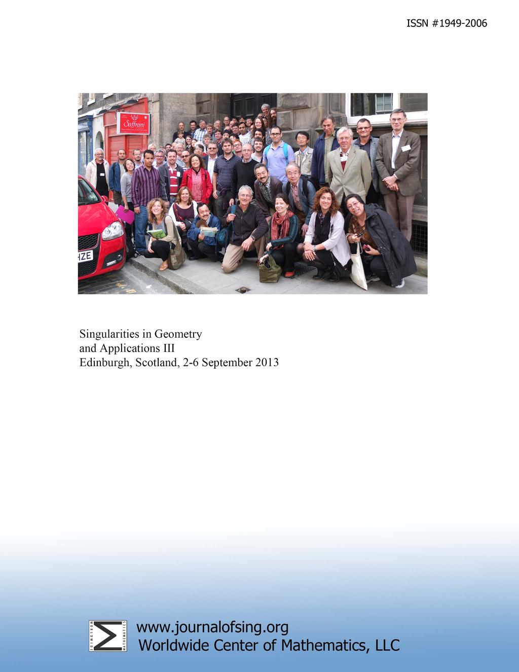
228