Mathematics for Economics MA course
|
|
|
- Alexis Kennedy
- 5 years ago
- Views:
Transcription
1 Mathematics for Economics MA course Simple Linear Regression Dr. Seetha Bandara
2 Simple Regression Simple linear regression is a statistical method that allows us to summarize and study relationships between two continuous (quantitative) variables: One variable, denoted x, is regarded as the predictor, explanatory, or independent variable. The other variable, denoted y, is regarded as the response, outcome, or dependent variable.
3 Introduction The primary goal of quantitative analysis is to use current information about a phenomenon to predict its future behavior. Current information is usually in the form of a set of data. In a simple case, when the data form a set of pairs of numbers, we may interpret them as representing the observed values of an independent (or predictor ) variable X and a dependent ( or response) variable Y. lot size Man-hours
4 Introduction Statistical relation between Lot size and Man-Hour The goal of the analyst who studies the data is to find a functional relation y f (x) between the response variable y and the predictor variable x. Man-Hour Lot size
5 Regression Function The statement that the relation between X and Y is statistical should be interpreted as providing the following guidelines: 1. Regard Y as a random variable. 2. For each X, take f (x) to be the expected value (i.e., mean value) of y. 3. Given that E (Y) denotes the expected value of Y, call the equation E( Y) f ( x) the regression function.
6 Pictorial Presentation of Linear Regression Model
7 Historical Origin of Regression Regression Analysis was first developed by Sir Francis Galton, who studied the relation between heights of sons and fathers. Heights of sons of both tall and short fathers appeared to revert or regress to the mean of the group.
8 Construction of Regression Models Selection of independent variables Since reality must be reduced to manageable proportions whenever we construct models, only a limited number of independent or predictor variables can or should be included in a regression model. Therefore a central problem is that of choosing the most important predictor variables. Functional form of regression relation Sometimes, relevant theory may indicate the appropriate functional form. More frequently, however, the functional form is not known in advance and must be decided once the data have been collected and analyzed. Scope of model In formulating a regression model, we usually need to restrict the coverage of model to some interval or region of values of the independent variables.
9 Uses of Regression Analysis Regression analysis serves Three major purposes. 1. Description 2. Control 3. Prediction The several purposes of regression analysis frequently overlap in practice
10 Formal Statement of the Model General regression model Y 0 1 X 1. 0, and 1 are parameters 2. X is a known constant 3. Deviations are independent N(o, 2 )
11 Meaning of Regression Coefficients The values of the regression parameters 0, and 1 are not known.we estimate them from data. 1 indicates the change in the mean response per unit increase in X.
12 Regression Line If the scatter plot of our sample data suggests a linear relationship between two variables i.e. y x 1 0 we can summarize the relationship by drawing a straight line on the plot. Least squares method give us the best estimated line for our set of sample data.
13 Regression Line We will write an estimated regression line based on sample data as yˆ b0 b1 x The method of least squares chooses the values for b 0, and b 1 to minimize the sum of squared errors SSE n n 2 ( y ˆ i yi ) i1 i1 2 y b b x 0 1
14 Regression Line Using calculus, we obtain estimating formulas: or n i n i i i n i n i n i i i i i n i i n i i i x x n y x y x n x x y y x x b ) ( ) ( ) )( ( b x y b 1 0 x y S S b r 1
15 Estimation of Mean Response Fitted regression line can be used to estimate the mean value of y for a given value of x. Example The weekly advertising expenditure (x) and weekly sales (y) are presented in the following table. y x
16 Point Estimation of Mean Response From previous table we have: n 10 y x The least squares estimates of the regression coefficients are: b n xy x x) ( x 2 xy n x y 10(818755) (564)(14365) 2 10(32604) (564) b (56.4)
17 Point Estimation of Mean Response The estimated regression function is: ŷ x Sales Expenditure This means that if the weekly advertising expenditure is increased by $1 we would expect the weekly sales to increase by $10.8.
18 Point Estimation of Mean Response Fitted values for the sample data are obtained by substituting the x value into the estimated regression function. For example if the advertising expenditure is $50, then the estimated Sales is: Sales (50) 1368 This is called the point estimate (forecast) of the mean response (sales).
19 Example:Retail sales and floor space It is customary in retail operations to asses the performance of stores partly in terms of their annual sales relative to their floor area (square feet). We might expect sales to increase linearly as stores get larger, with of course individual variation among stores of the same size. The regression model for a population of stores says that SALES = AREA +
20 Example:Retail sales and floor space The slope 1 is as usual a rate of change: it is the expected increase in annual sales associated with each additional square foot of floor space. The intercept 0 is needed to describe the line but has no statistical importance because no stores have area close to zero. Floor space does not completely determine sales. The term in the model accounts for difference among individual stores with the same floor space. A store s location, for example, is important.
21 Residual The difference between the observed value y i and the corresponding fitted value. ŷ i e i y i yˆ i Residuals are highly useful for studying whether a given regression model is appropriate for the data at hand.
22 Example: weekly advertising expenditure y x y-hat Residual (e)
23 Estimation of the variance of the error terms, 2 The variance 2 of the error terms i in the regression model needs to be estimated for a variety of purposes. It gives an indication of the variability of the probability distributions of y. It is needed for making inference concerning regression function and the prediction of y.
24 Regression Standard Error To estimate we work with the variance and take the square root to obtain the standard deviation. For simple linear regression the estimate of 2 is the average squared residual. s y To estimate, use ˆ x ei ( yi yi ) n 2 n 2 s 2 y. x sy. x s estimates the standard deviation of the error term in the statistical model for simple linear regression. 2
25 Regression Standard Error y x y-hat Residual (e) square(e) y-hat = X total S y.x
26 Basic Assumptions of a Regression Model A regression model is based on the following assumptions: 1. There is a probability distribution of Y for each level of X. 2. Given that µ y is the mean value of Y, the standard form of the model is f ( x ) y where is a random variable with a normal distribution with mean 0 and standard deviation.
27 Conditions for Regression Inference You can fit a least-squares line to any set of explanatory-response data when both variables are quantitative. If the scatter plot doesn t show an approximately linear pattern, the fitted line may be almost useless.
28 Conditions for Regression Inference The simple linear regression model, which is the basis for inference, imposes several conditions. We should verify these conditions before proceeding with inference. The conditions concern the population, but we can observe only our sample.
29 Conditions for Regression Inference In doing Inference, we assume: 1. The sample is an SRS from the population. 2. There is a linear relationship in the population. 1. We can not observe the population, so we check the scatter plot of the sample data. 3. The standard deviation of the responses about the population line is the same for all values of the explanatory variable. 1. The spread of observations above and below the least-squares line should be roughly uniform as x varies.
30 Conditions for Regression Inference Plotting the residuals against the explanatory variable is helpful in checking these conditions because a residual plot magnifies patterns.
31 Analysis of Residual To examine whether the regression model is appropriate for the data being analyzed, we can check the residual plots. Residual plots are: Plot a histogram of the residuals Plot residuals against the fitted values. Plot residuals against the independent variable. Plot residuals over time if the data are chronological.
32 Analysis of Residual A histogram of the residuals provides a check on the normality assumption. A Normal quantile plot of the residuals can also be used to check the Normality assumptions. Regression Inference is robust against moderate lack of Normality. On the other hand, outliers and influential observations can invalidate the results of inference for regression Plot of residuals against fitted values or the independent variable can be used to check the assumption of constant variance and the aptness of the model.
33 Analysis of Residual Plot of residuals against time provides a check on the independence of the error terms assumption. Assumption of independence is the most critical one.
34 Residual plots The residuals should have no systematic pattern. The residual plot to right shows a scatter of the points with no individual observations or systematic change as x increases. Residuals Degree Days Residual Plot Degree Days

35 Residual plots The points in this residual plot have a curve pattern, so a straight line fits poorly

36 Residual plots The points in this plot show more spread for larger values of the explanatory variable x, so prediction will be less accurate when x is large.
37 Variable transformations If the residual plot suggests that the variance is not constant, a transformation can be used to stabilize the variance. If the residual plot suggests a non linear relationship between x and y, a transformation may reduce it to one that is approximately linear. Common linearizing transformations are: 1 x, log( x) Variance stabilizing transformations are: 1, y log( y), y, y 2
38 Inference about the Regression Model When a scatter plot shows a linear relationship between a quantitative explanatory variable x and a quantitative response variable y, we can use the least square line fitted to the data to predict y for a give value of x. Now we want to do tests and confidence intervals in this setting.
39 Inference about the Regression Model We think of the least square line we calculated from a sample as an estimate of a regression line for the population. Just as the sample mean population mean µ. x is an estimate of the
40 Inference about the Regression Model We will write the population regression line as 0 1 x The numbers and are parameters that describe the 0 1 population. We will write the least-squares line fitted to sample data as b0 b1 x This notation reminds us that the intercept b 0 of the fitted line estimates the intercept 0 of the population line, and the slope b 1 estimates the slope 1.
41 Confidence Intervals and Significance Tests In our previous lectures we presented confidence intervals and significance tests for means and differences in means.in each case, inference rested on the standard error s of the estimates and on t or z distributions. Inference for the slope and intercept in linear regression is similar in principal, although the recipes are more complicated. All confidence intervals, for example, have the form estimate t* Se estimate t* is a critical value of a t distribution.
42 Confidence Intervals and Significance Tests Confidence intervals and tests for the slope and intercept are based on the sampling distributions of the estimates b 1 and b 0. Here are the facts: If the simple linear regression model is true, each of b 0 and b 1 has a Normal distribution. The mean of b 0 is 0 and the mean of b 1 is 1. That is, the intercept and slope of the fitted line are unbiased estimators of the intercept and slope of the population regression line.
43 Confidence Intervals and Significance Tests The standard deviations of b 0 and b 1 are multiples of the model standard deviation. 2 1 ) ( ) ( 1 x x s b S SE b n i i b x x x n s b S SE ) ( 1 ) ( 0

44 Confidence Intervals and Significance Tests
45 Example:Weekly Advertising Expenditure Let us return to the Weekly advertising expenditure and weekly sales example. Management is interested in testing whether or not there is a linear association between advertising expenditure and weekly sales, using regression model. Use =.05
46 Example:Weekly Advertising Expenditure Hypothesis: H Decision Rule: Reject H 0 if or 0 H a t : : t t t ;8 t. 025;8 t
47 Example:Weekly Advertising Expenditure Test statistic: t b1 S( b 1 ) S y. x S( b ) ( x x) b t
48 Example:Weekly Advertising Expenditure Conclusion: Since t =4.5 > then we reject H 0. There is a linear association between advertising expenditure and weekly sales.
49 Confidence interval for 1 b 1 t b ( ; n2) 2 ( S( 1)) Now that our test showed that there is a linear association between advertising expenditure and weekly sales, the management wishes an estimate of 1 with a 95% confidence coefficient.
50 Confidence interval for 1 For a 95 percent confidence coefficient, we require t (.025; 8). From table B in appendix III, we find t(.025; 8) = The 95% confidence interval is: b 1 t 10.8 ( ; n2) 2 ( S( b1 )) 2.306(2.38) (5.31, 16.3)
51 Example: Do wages rise with experience? Many factors affect the wages of workers: the industry they work in, their type of job, their education and their experience, and changes in general levels of wages. We will look at a sample of 59 married women who hold customer service jobs in Indiana banks. The following table gives their weekly wages at a specific point in time also their length of service with their employer, in month. The size of the place of work is recorded simply as large (100 or more workers) or small. Because industry, job type, and the time of measurement are the same for all 59 subjects, we expect to see a clear relationship between wages and length of service.
52 Example: Do wages rise with experience?

53 Example: Do wages rise with experience?
54 Example: Do wages rise with experience? From previous table we have: n 59 y x 4159 y x xy The least squares estimates of the regression coefficients are: b 1 r s s y x b 0 y bx
55 Example: Do wages rise with experience? What is the least-squares regression line for predicting Wages from Length of service (Los)? Suppose a woman has been with her bank for 125 months. What do you predict she will earn? If her actual wages are $433, then what is her residual? The sum of squared residuals for the entire sample is 59 ( y ˆ ) 2 i y i i1
56 Example: Do wages rise with experience? Do wages rise with experience? The hypotheses are: H 0 : 1 = 0, H a : 1 > 0 The test statistics The P- value is: Conclusion: b1 t SE b 1
57 Example: Do wages rise with experience? A 95% confidence interval for the average increase in wages per month of stay for the regression line in the population of all married female customer service workers in Indiana bank is b t * SE 1 1 b The t distribution for this problem has n-2 = 57 degrees of freedom
58 Example: Do wages rise with experience? Regression calculations in Practice are always done by software. The computer out put for the case study is given in the following slide.

59 Example: Do wages rise with experience?
60 Using the regression Line One of the most common reasons to fit a line to data is to predict the response to a particular value of the explanatory variable. In our example, the least square line for predicting the weekly earnings for female bank customer service workers from their length of service is yˆ x
61 Using the regression Line For a length of service of 125 months, our leastsquares regression equation gives yˆ (.5905)(125) $423 per week There are two different uses of this prediction. We can estimate the mean earnings of all workers in the subpopulation of workers with 125 months on the job. We can predict the earnings of one individual worker with 125 months of service.
62 Using the regression Line For each use, the actual prediction is the same,.but the margin of error is different for the two cases. To estimate the mean response, we use a confidence * interval. y 0 1x To estimate an individual response y, we use prediction interval. yˆ $423 A prediction interval estimates a single random response y rather than a parameter like µ y
63 Using the regression Line The main distinction is that it is harder to predict for an individual than for the mean of a population of individuals. Each interval has the usual form y ˆ t * SE The margin of error for the prediction interval is wider than the margin of error for the confidence interval.
64 Using the regression Line The standard error for estimating the mean response when the explanatory variable x takes the value x* is:
65 Using the regression Line The standard error for predicting an individual response when the explanatory variable x takes the value x* is:
66 Prediction of a new response ( ) We now consider the prediction of a new observation y corresponding to a given level x of the independent variable. In our advertising expenditure and weekly sales, the management wishes to predict the weekly sales corresponding to the advertising expenditure of x = $50. ŷ
67 Interval Estimation of a new response ( ) The following formula gives us the point estimator (forecast) for y. yˆ b0 b1 x 1- % prediction interval for a new observation ŷ is: yˆ t ( S ) Where S f ( ; n2) ( x x) S y. x 1 2 n ( x x) f ŷ
68 Example In our advertising expenditure and weekly sales, the management wishes to predict the weekly sales if the advertising expenditure is $50 with a 90 % prediction interval. S S yˆ f f (50) 1368 S y. x n ( x x) ( x x) We require t(.05; 8) = ( )
69 Example The 90% prediction interval is: ˆ t(.05;8) y ( S (72.11) (1233.9, ) f )
70 Analysis of variance approach to Regression analysis Analysis of Variance is the term for statistical analyses that break down the variation in data into separate pieces that correspond to different sources of variation. It is based on the partitioning of sums of squares and degrees of freedom associated with the response variable. In the regression setting, the observed variation in the responses (y i ) comes from two sources.
71 Analysis of variance approach to Regression analysis Consider the weekly advertising expenditure and the weekly sales example. There is variation in the amount ($) of weekly sales, as in all statistical data. The variation of the y i is conventionally measured in terms of the deviations: y i y
72 Analysis of variance approach to Regression analysis The measure of total variation, denoted by SST, is the sum of the squared deviations: SST ( y y) If SST = 0, all observations are the same(no variability). The greater is SST, the greater is the variation among the y values. When we use the regression model, the measure of variation is that of the y observations variability around the fitted line: y i 2 ˆ i y i
73 Analysis of variance approach to Regression analysis The measure of variation in the data around the fitted regression line is the sum of squared deviations (error), denoted SSE: SSE y i yˆ ( i For our Weekly expenditure example SSE = SST = What accounts for the substantial difference between these two sums of squares? ) 2
74 Analysis of variance approach to Regression analysis The difference is another sum of squares: SSR ( yˆ y) i SSR stands for regression sum of squares. SSR is the variation among the predicted responses ŷ i. The predicted responses lie on the least-square line. They show how y moves in response to x. The larger is SSR relative to SST, the greater is the role of regression line in explaining the total variability in y observations. 2
75 Analysis of variance approach to Regression analysis In our example: SSR SST SSE This indicates that most of variability in weekly sales can be explained by the relation between the weekly advertising expenditure and the weekly sales.
76 Formal Development of the Partitioning We can decompose the total variability in the observations y i as follows: y y yˆ y y yˆ i i The total deviation y i y can be viewed as the sum of two components: The deviation of the fitted value around the mean y. The deviation of y i around the fitted regression line. i i ŷ i
77 Formal Development of the Partitioning Skipping quite a bit of messy algebra, we just state that this analysis of variance equation always holds: ( y ) ( ˆ ) ( ˆ i y yi y yi yi ) Breakdown of degree of freedom: n 11 ( n 2)
78 Mean squares A sum of squares divided by its degrees of freedom is called a mean square (MS) Regression mean square (MSR) MSR SSR 1 Error mean square (MSE) SSE MSE n 2 Note: mean squares are not additive.
79 Mean squares In our example: MSR SSR SSE MSE n
80 Analysis of Variance Table The breakdowns of the total sum of squares and associated degrees of freedom are displayed in a table called analysis of variance table (ANOVA table) Source of Variation SS df MS F-Test Regression SSR 1 MSR =SSR/1 MSR/MSE Error SSE n-2 MSE Total SST n-1 =SSE/(n-2)
81 Analysis of Variance Table In our weekly advertising expenditure and weekly sales example the ANOVA table is: Source of variation SS df MS Regression Error Total
82 Analysis of Variance Table The Analysis of Variance table reports in a different way quantities such as r2 and s that are needed in regression analysis. It also reports in a different way the test for the overall significance of the regression. If regression on x has no value for predicting y, we expect the slope of the population regression line to be close to 0.
83 Analysis of Variance Table That is the null hypothesis of no linear relationship is: H 0 0 : 1 We standardize the slope of the leastsquares line to get a t statistic.
84 F-Test for 1 = 0 versus 1 0 The analysis of variance approach starts with sums of squares. If regression on x has no value for predicting y, we expect the SSR to be only a small part of the SST, most of which will be made of the SSE. The proper way to standardize this comparison is to use the ratio F MSR MSE
85 F-Test for 1 = 0 versus 1 0 In order to be able to construct a statistical decision rule, we need to know the distribution of our test statistic F. When H 0 is true, our test statistic, F, follows the F- distribution with 1, and n-2 degrees of freedom. Table C-5 on page 513 of your text gives the critical values of the F-distribution at = 0.05 and.01.
86 F-Test for 1 = 0 versus 1 0 Construction of decision rule: At = 5% level Reject H 0 if F F( ;1, n 2) Large values of F support H a and Values of F near 1 support H 0.
87 F-Test for 1 = 0 versus 1 0 Using our example again, let us repeat the earlier test on 1. This time we will use the F-test. The null and alternative hypothesis are: H : 0 Let =.05. Since n=10, we require F(.05; 1, 8). From table 5-3 we find that F(.05; 1, 8) = Therefore the decision rule is: Reject H 0 if: 0 H a : F 5.32
88 F-Test for 1 = 0 versus 1 0 From ANOVA table we have MSR = MSE = Our test statistic F is: Decision: F Since 20.47> 5.32, we reject H 0, that is there is a linear association between weekly advertising expenditure and weekly sales.
89 F-Test for 1 = 0 versus 1 0 Equivalence of F Test and t Test: For given level, the F test of 1 = 0 versus 1 0 is equivalent algebraically to the two sided t- test. Thus, at a given level, we can use either the t-test or the F-test for testing 1 = 0 versus 1 0. The t-test is more flexible since it can be used for one sided test as well.
90 Analysis of Variance Table The complete ANOVA table for our example is: Source of Variation SS df MS F-Test Regression Error Total
91 Computer Output The EXCEL out put for our example is: SUMMARY OUTPUT Regression Statistics Multiple R R Square Adjusted R Square Standard Error Observations 10 ANOVA df SS MS F Significance F Regression Residual Total Coefficients Standard Error t Stat P-value Lower 95% Upper 95% Intercept AD-Expen (X)
92 Coefficient of Determination Recall that SST measures the total variations in y i when no account of the independent variable x is taken. SSE measures the variation in the y i when a regression model with the independent variable x is used. A natural measure of the effect of x in reducing the variation in y can be defined as: R 2 SST SSE SSR 1 SST SST SSE SST
93 Coefficient of Determination R 2 is called the coefficient of determination. 0 SSE SST, it follows that: 0 R 2 1 We may interpret R 2 as the proportionate reduction of total variability in y associated with the use of the independent variable x. The larger is R 2, the more is the total variation of y reduced by including the variable x in the model.
94 Coefficient of Determination If all the observations fall on the fitted regression line, SSE = 0 and R 2 = 1. If the slope of the fitted regression line b 1 = 0 so that yˆ, SSE=SST and R 2 i y = 0. The closer R 2 is to 1, the greater is said to be the degree of linear association between x and y. The square root of R 2 is called the coefficient of correlation. r 2 R
95 Correlation Coefficient Recall that the algebraic expression for the correlation coefficient is ) ( ) ( ) ( ) ( ) )( ( y y n x x n y x xy n r y y x x y y x x r
96
97
98
99
Inference for the Regression Coefficient
 Inference for the Regression Coefficient Recall, b 0 and b 1 are the estimates of the slope β 1 and intercept β 0 of population regression line. We can shows that b 0 and b 1 are the unbiased estimates
Inference for Regression Inference about the Regression Model and Using the Regression Line, with Details. Section 10.1, 2, 3
 Inference for Regression Inference about the Regression Model and Using the Regression Line, with Details Section 10.1, 2, 3 Basic components of regression setup Target of inference: linear dependency
Correlation Analysis
 Simple Regression Correlation Analysis Correlation analysis is used to measure strength of the association (linear relationship) between two variables Correlation is only concerned with strength of the
Chapter 14 Student Lecture Notes Department of Quantitative Methods & Information Systems. Business Statistics. Chapter 14 Multiple Regression
 Chapter 14 Student Lecture Notes 14-1 Department of Quantitative Methods & Information Systems Business Statistics Chapter 14 Multiple Regression QMIS 0 Dr. Mohammad Zainal Chapter Goals After completing
Statistics for Managers using Microsoft Excel 6 th Edition
 Statistics for Managers using Microsoft Excel 6 th Edition Chapter 13 Simple Linear Regression 13-1 Learning Objectives In this chapter, you learn: How to use regression analysis to predict the value of
Basic Business Statistics 6 th Edition
 Basic Business Statistics 6 th Edition Chapter 12 Simple Linear Regression Learning Objectives In this chapter, you learn: How to use regression analysis to predict the value of a dependent variable based
Estimating σ 2. We can do simple prediction of Y and estimation of the mean of Y at any value of X.
 Estimating σ 2 We can do simple prediction of Y and estimation of the mean of Y at any value of X. To perform inferences about our regression line, we must estimate σ 2, the variance of the error term.
Chapter 16. Simple Linear Regression and dcorrelation
 Chapter 16 Simple Linear Regression and dcorrelation 16.1 Regression Analysis Our problem objective is to analyze the relationship between interval variables; regression analysis is the first tool we will
Inferences for Regression
 Inferences for Regression An Example: Body Fat and Waist Size Looking at the relationship between % body fat and waist size (in inches). Here is a scatterplot of our data set: Remembering Regression In
Inference for Regression Simple Linear Regression
 Inference for Regression Simple Linear Regression IPS Chapter 10.1 2009 W.H. Freeman and Company Objectives (IPS Chapter 10.1) Simple linear regression p Statistical model for linear regression p Estimating
The Multiple Regression Model
 Multiple Regression The Multiple Regression Model Idea: Examine the linear relationship between 1 dependent (Y) & or more independent variables (X i ) Multiple Regression Model with k Independent Variables:
Regression Models. Chapter 4. Introduction. Introduction. Introduction
 Chapter 4 Regression Models Quantitative Analysis for Management, Tenth Edition, by Render, Stair, and Hanna 008 Prentice-Hall, Inc. Introduction Regression analysis is a very valuable tool for a manager
Chapter 16. Simple Linear Regression and Correlation
 Chapter 16 Simple Linear Regression and Correlation 16.1 Regression Analysis Our problem objective is to analyze the relationship between interval variables; regression analysis is the first tool we will
Ch 2: Simple Linear Regression
 Ch 2: Simple Linear Regression 1. Simple Linear Regression Model A simple regression model with a single regressor x is y = β 0 + β 1 x + ɛ, where we assume that the error ɛ is independent random component
Chapter 4. Regression Models. Learning Objectives
 Chapter 4 Regression Models To accompany Quantitative Analysis for Management, Eleventh Edition, by Render, Stair, and Hanna Power Point slides created by Brian Peterson Learning Objectives After completing
Business Statistics. Chapter 14 Introduction to Linear Regression and Correlation Analysis QMIS 220. Dr. Mohammad Zainal
 Department of Quantitative Methods & Information Systems Business Statistics Chapter 14 Introduction to Linear Regression and Correlation Analysis QMIS 220 Dr. Mohammad Zainal Chapter Goals After completing
Chapter 7 Student Lecture Notes 7-1
 Chapter 7 Student Lecture Notes 7- Chapter Goals QM353: Business Statistics Chapter 7 Multiple Regression Analysis and Model Building After completing this chapter, you should be able to: Explain model
Chapter 14 Student Lecture Notes 14-1
 Chapter 14 Student Lecture Notes 14-1 Business Statistics: A Decision-Making Approach 6 th Edition Chapter 14 Multiple Regression Analysis and Model Building Chap 14-1 Chapter Goals After completing this
Inference for Regression Inference about the Regression Model and Using the Regression Line
 Inference for Regression Inference about the Regression Model and Using the Regression Line PBS Chapter 10.1 and 10.2 2009 W.H. Freeman and Company Objectives (PBS Chapter 10.1 and 10.2) Inference about
Inference for Regression
 Inference for Regression Section 9.4 Cathy Poliak, Ph.D. cathy@math.uh.edu Office in Fleming 11c Department of Mathematics University of Houston Lecture 13b - 3339 Cathy Poliak, Ph.D. cathy@math.uh.edu
Chapter 3 Multiple Regression Complete Example
 Department of Quantitative Methods & Information Systems ECON 504 Chapter 3 Multiple Regression Complete Example Spring 2013 Dr. Mohammad Zainal Review Goals After completing this lecture, you should be
9. Linear Regression and Correlation
 9. Linear Regression and Correlation Data: y a quantitative response variable x a quantitative explanatory variable (Chap. 8: Recall that both variables were categorical) For example, y = annual income,
Econ 3790: Business and Economics Statistics. Instructor: Yogesh Uppal
 Econ 3790: Business and Economics Statistics Instructor: Yogesh Uppal yuppal@ysu.edu Sampling Distribution of b 1 Expected value of b 1 : Variance of b 1 : E(b 1 ) = 1 Var(b 1 ) = σ 2 /SS x Estimate of
Ch 13 & 14 - Regression Analysis
 Ch 3 & 4 - Regression Analysis Simple Regression Model I. Multiple Choice:. A simple regression is a regression model that contains a. only one independent variable b. only one dependent variable c. more
The simple linear regression model discussed in Chapter 13 was written as
 1519T_c14 03/27/2006 07:28 AM Page 614 Chapter Jose Luis Pelaez Inc/Blend Images/Getty Images, Inc./Getty Images, Inc. 14 Multiple Regression 14.1 Multiple Regression Analysis 14.2 Assumptions of the Multiple
Keller: Stats for Mgmt & Econ, 7th Ed July 17, 2006
 Chapter 17 Simple Linear Regression and Correlation 17.1 Regression Analysis Our problem objective is to analyze the relationship between interval variables; regression analysis is the first tool we will
Chapter 4: Regression Models
 Sales volume of company 1 Textbook: pp. 129-164 Chapter 4: Regression Models Money spent on advertising 2 Learning Objectives After completing this chapter, students will be able to: Identify variables,
Chapter 14 Simple Linear Regression (A)
") Chapter 14 Simple Linear Regression (A) 1. Characteristics Managerial decisions often are based on the relationship between two or more variables. can be used to develop an equation showing how the variables
Chapter 14 Simple Linear Regression (A) 1. Characteristics Managerial decisions often are based on the relationship between two or more variables. can be used to develop an equation showing how the variables
LI EAR REGRESSIO A D CORRELATIO
 CHAPTER 6 LI EAR REGRESSIO A D CORRELATIO Page Contents 6.1 Introduction 10 6. Curve Fitting 10 6.3 Fitting a Simple Linear Regression Line 103 6.4 Linear Correlation Analysis 107 6.5 Spearman s Rank Correlation
Section 3: Simple Linear Regression
 Section 3: Simple Linear Regression Carlos M. Carvalho The University of Texas at Austin McCombs School of Business http://faculty.mccombs.utexas.edu/carlos.carvalho/teaching/ 1 Regression: General Introduction
(ii) Scan your answer sheets INTO ONE FILE only, and submit it in the drop-box.
 Scan your answer sheets INTO ONE FILE only, and submit it in the drop-box.") FINAL EXAM ** Two different ways to submit your answer sheet (i) Use MS-Word and place it in a drop-box. (ii) Scan your answer sheets INTO ONE FILE only, and submit it in the drop-box. Deadline: December
FINAL EXAM ** Two different ways to submit your answer sheet (i) Use MS-Word and place it in a drop-box. (ii) Scan your answer sheets INTO ONE FILE only, and submit it in the drop-box. Deadline: December
STAT 350 Final (new Material) Review Problems Key Spring 2016
 Review Problems Key Spring 2016") 1. The editor of a statistics textbook would like to plan for the next edition. A key variable is the number of pages that will be in the final version. Text files are prepared by the authors using LaTeX,
1. The editor of a statistics textbook would like to plan for the next edition. A key variable is the number of pages that will be in the final version. Text files are prepared by the authors using LaTeX,
27. SIMPLE LINEAR REGRESSION II
 27. SIMPLE LINEAR REGRESSION II The Model In linear regression analysis, we assume that the relationship between X and Y is linear. This does not mean, however, that Y can be perfectly predicted from X.
Sociology 6Z03 Review II
 Sociology 6Z03 Review II John Fox McMaster University Fall 2016 John Fox (McMaster University) Sociology 6Z03 Review II Fall 2016 1 / 35 Outline: Review II Probability Part I Sampling Distributions Probability
LECTURE 6. Introduction to Econometrics. Hypothesis testing & Goodness of fit
 LECTURE 6 Introduction to Econometrics Hypothesis testing & Goodness of fit October 25, 2016 1 / 23 ON TODAY S LECTURE We will explain how multiple hypotheses are tested in a regression model We will define
Lecture 2 Simple Linear Regression STAT 512 Spring 2011 Background Reading KNNL: Chapter 1
 Lecture Simple Linear Regression STAT 51 Spring 011 Background Reading KNNL: Chapter 1-1 Topic Overview This topic we will cover: Regression Terminology Simple Linear Regression with a single predictor
INFERENCE FOR REGRESSION
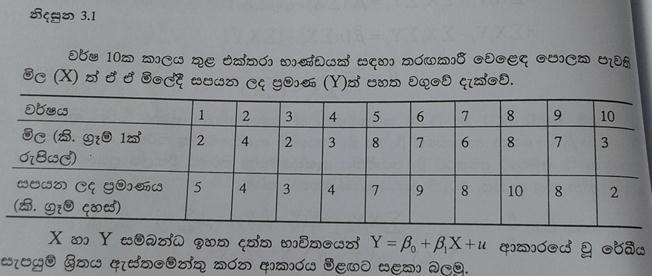
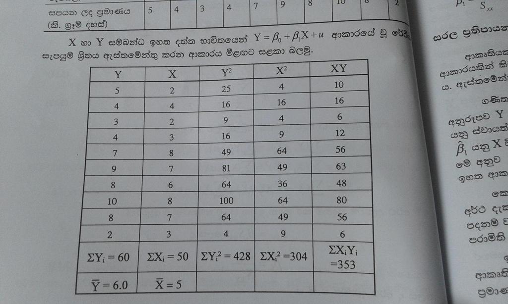
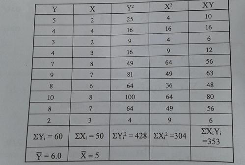
 CHAPTER 3 INFERENCE FOR REGRESSION OVERVIEW In Chapter 5 of the textbook, we first encountered regression. The assumptions that describe the regression model we use in this chapter are the following. We
Basic Business Statistics, 10/e
 Chapter 4 4- Basic Business Statistics th Edition Chapter 4 Introduction to Multiple Regression Basic Business Statistics, e 9 Prentice-Hall, Inc. Chap 4- Learning Objectives In this chapter, you learn:
STAT Chapter 11: Regression
 STAT 515 -- Chapter 11: Regression Mostly we have studied the behavior of a single random variable. Often, however, we gather data on two random variables. We wish to determine: Is there a relationship
STAT5044: Regression and Anova. Inyoung Kim
 STAT5044: Regression and Anova Inyoung Kim 2 / 47 Outline 1 Regression 2 Simple Linear regression 3 Basic concepts in regression 4 How to estimate unknown parameters 5 Properties of Least Squares Estimators:
Ordinary Least Squares Regression Explained: Vartanian
 Ordinary Least Squares Regression Explained: Vartanian When to Use Ordinary Least Squares Regression Analysis A. Variable types. When you have an interval/ratio scale dependent variable.. When your independent
Simple Linear Regression
 9-1 l Chapter 9 l Simple Linear Regression 9.1 Simple Linear Regression 9.2 Scatter Diagram 9.3 Graphical Method for Determining Regression 9.4 Least Square Method 9.5 Correlation Coefficient and Coefficient
Econ 3790: Statistics Business and Economics. Instructor: Yogesh Uppal
 Econ 3790: Statistics Business and Economics Instructor: Yogesh Uppal Email: yuppal@ysu.edu Chapter 14 Covariance and Simple Correlation Coefficient Simple Linear Regression Covariance Covariance between
Simple Linear Regression. Material from Devore s book (Ed 8), and Cengagebrain.com
, and Cengagebrain.com") 12 Simple Linear Regression Material from Devore s book (Ed 8), and Cengagebrain.com The Simple Linear Regression Model The simplest deterministic mathematical relationship between two variables x and
12 Simple Linear Regression Material from Devore s book (Ed 8), and Cengagebrain.com The Simple Linear Regression Model The simplest deterministic mathematical relationship between two variables x and
Simple Linear Regression
 Simple Linear Regression ST 430/514 Recall: A regression model describes how a dependent variable (or response) Y is affected, on average, by one or more independent variables (or factors, or covariates)
4.1 Least Squares Prediction 4.2 Measuring Goodness-of-Fit. 4.3 Modeling Issues. 4.4 Log-Linear Models
 4.1 Least Squares Prediction 4. Measuring Goodness-of-Fit 4.3 Modeling Issues 4.4 Log-Linear Models y = β + β x + e 0 1 0 0 ( ) E y where e 0 is a random error. We assume that and E( e 0 ) = 0 var ( e
Correlation and the Analysis of Variance Approach to Simple Linear Regression
 Correlation and the Analysis of Variance Approach to Simple Linear Regression Biometry 755 Spring 2009 Correlation and the Analysis of Variance Approach to Simple Linear Regression p. 1/35 Correlation
Regression Analysis II
 Regression Analysis II Measures of Goodness of fit Two measures of Goodness of fit Measure of the absolute fit of the sample points to the sample regression line Standard error of the estimate An index
BNAD 276 Lecture 10 Simple Linear Regression Model
 1 / 27 BNAD 276 Lecture 10 Simple Linear Regression Model Phuong Ho May 30, 2017 2 / 27 Outline 1 Introduction 2 3 / 27 Outline 1 Introduction 2 4 / 27 Simple Linear Regression Model Managerial decisions
Lecture 15 Multiple regression I Chapter 6 Set 2 Least Square Estimation The quadratic form to be minimized is
 Lecture 15 Multiple regression I Chapter 6 Set 2 Least Square Estimation The quadratic form to be minimized is Q = (Y i β 0 β 1 X i1 β 2 X i2 β p 1 X i.p 1 ) 2, which in matrix notation is Q = (Y Xβ) (Y
We like to capture and represent the relationship between a set of possible causes and their response, by using a statistical predictive model.
 Statistical Methods in Business Lecture 5. Linear Regression We like to capture and represent the relationship between a set of possible causes and their response, by using a statistical predictive model.
Lecture 10 Multiple Linear Regression
 Lecture 10 Multiple Linear Regression STAT 512 Spring 2011 Background Reading KNNL: 6.1-6.5 10-1 Topic Overview Multiple Linear Regression Model 10-2 Data for Multiple Regression Y i is the response variable
CHAPTER 5 LINEAR REGRESSION AND CORRELATION
 CHAPTER 5 LINEAR REGRESSION AND CORRELATION Expected Outcomes Able to use simple and multiple linear regression analysis, and correlation. Able to conduct hypothesis testing for simple and multiple linear
Lecture 18: Simple Linear Regression
 Lecture 18: Simple Linear Regression BIOS 553 Department of Biostatistics University of Michigan Fall 2004 The Correlation Coefficient: r The correlation coefficient (r) is a number that measures the strength
Formal Statement of Simple Linear Regression Model
 Formal Statement of Simple Linear Regression Model Y i = β 0 + β 1 X i + ɛ i Y i value of the response variable in the i th trial β 0 and β 1 are parameters X i is a known constant, the value of the predictor
Business Statistics. Lecture 9: Simple Regression
 Business Statistics Lecture 9: Simple Regression 1 On to Model Building! Up to now, class was about descriptive and inferential statistics Numerical and graphical summaries of data Confidence intervals
STA121: Applied Regression Analysis
 STA121: Applied Regression Analysis Linear Regression Analysis - Chapters 3 and 4 in Dielman Artin Department of Statistical Science September 15, 2009 Outline 1 Simple Linear Regression Analysis 2 Using
Multiple Regression. Inference for Multiple Regression and A Case Study. IPS Chapters 11.1 and W.H. Freeman and Company
 Multiple Regression Inference for Multiple Regression and A Case Study IPS Chapters 11.1 and 11.2 2009 W.H. Freeman and Company Objectives (IPS Chapters 11.1 and 11.2) Multiple regression Data for multiple
Simple Linear Regression. (Chs 12.1, 12.2, 12.4, 12.5)
") 10 Simple Linear Regression (Chs 12.1, 12.2, 12.4, 12.5) Simple Linear Regression Rating 20 40 60 80 0 5 10 15 Sugar 2 Simple Linear Regression Rating 20 40 60 80 0 5 10 15 Sugar 3 Simple Linear Regression
10 Simple Linear Regression (Chs 12.1, 12.2, 12.4, 12.5) Simple Linear Regression Rating 20 40 60 80 0 5 10 15 Sugar 2 Simple Linear Regression Rating 20 40 60 80 0 5 10 15 Sugar 3 Simple Linear Regression
Lectures on Simple Linear Regression Stat 431, Summer 2012
 Lectures on Simple Linear Regression Stat 43, Summer 0 Hyunseung Kang July 6-8, 0 Last Updated: July 8, 0 :59PM Introduction Previously, we have been investigating various properties of the population
Six Sigma Black Belt Study Guides
 Six Sigma Black Belt Study Guides 1 www.pmtutor.org Powered by POeT Solvers Limited. Analyze Correlation and Regression Analysis 2 www.pmtutor.org Powered by POeT Solvers Limited. Variables and relationships
Chapter 13 Student Lecture Notes Department of Quantitative Methods & Information Systems. Business Statistics
 Chapter 13 Student Lecture Notes 13-1 Department of Quantitative Methods & Information Sstems Business Statistics Chapter 14 Introduction to Linear Regression and Correlation Analsis QMIS 0 Dr. Mohammad
Data Analysis and Statistical Methods Statistics 651
 y 1 2 3 4 5 6 7 x Data Analysis and Statistical Methods Statistics 651 http://www.stat.tamu.edu/~suhasini/teaching.html Lecture 32 Suhasini Subba Rao Previous lecture We are interested in whether a dependent
Linear models and their mathematical foundations: Simple linear regression
 Linear models and their mathematical foundations: Simple linear regression Steffen Unkel Department of Medical Statistics University Medical Center Göttingen, Germany Winter term 2018/19 1/21 Introduction
Lecture 11: Simple Linear Regression
 Lecture 11: Simple Linear Regression Readings: Sections 3.1-3.3, 11.1-11.3 Apr 17, 2009 In linear regression, we examine the association between two quantitative variables. Number of beers that you drink
AMS 315/576 Lecture Notes. Chapter 11. Simple Linear Regression
 AMS 315/576 Lecture Notes Chapter 11. Simple Linear Regression 11.1 Motivation A restaurant opening on a reservations-only basis would like to use the number of advance reservations x to predict the number
Regression Analysis. BUS 735: Business Decision Making and Research. Learn how to detect relationships between ordinal and categorical variables.
 Regression Analysis BUS 735: Business Decision Making and Research 1 Goals of this section Specific goals Learn how to detect relationships between ordinal and categorical variables. Learn how to estimate
Variance Decomposition and Goodness of Fit
 Variance Decomposition and Goodness of Fit 1. Example: Monthly Earnings and Years of Education In this tutorial, we will focus on an example that explores the relationship between total monthly earnings
Regression Analysis. Regression: Methodology for studying the relationship among two or more variables
 Regression Analysis Regression: Methodology for studying the relationship among two or more variables Two major aims: Determine an appropriate model for the relationship between the variables Predict the
SIMPLE REGRESSION ANALYSIS. Business Statistics
 SIMPLE REGRESSION ANALYSIS Business Statistics CONTENTS Ordinary least squares (recap for some) Statistical formulation of the regression model Assessing the regression model Testing the regression coefficients
Lecture 9: Linear Regression
 Lecture 9: Linear Regression Goals Develop basic concepts of linear regression from a probabilistic framework Estimating parameters and hypothesis testing with linear models Linear regression in R Regression
PubH 7405: REGRESSION ANALYSIS. MLR: INFERENCES, Part I
 PubH 7405: REGRESSION ANALYSIS MLR: INFERENCES, Part I TESTING HYPOTHESES Once we have fitted a multiple linear regression model and obtained estimates for the various parameters of interest, we want to
ECON 450 Development Economics
 ECON 450 Development Economics Statistics Background University of Illinois at Urbana-Champaign Summer 2017 Outline 1 Introduction 2 3 4 5 Introduction Regression analysis is one of the most important
Objectives Simple linear regression. Statistical model for linear regression. Estimating the regression parameters
 Objectives 10.1 Simple linear regression Statistical model for linear regression Estimating the regression parameters Confidence interval for regression parameters Significance test for the slope Confidence
Chapter 10. Regression. Understandable Statistics Ninth Edition By Brase and Brase Prepared by Yixun Shi Bloomsburg University of Pennsylvania
 Chapter 10 Regression Understandable Statistics Ninth Edition By Brase and Brase Prepared by Yixun Shi Bloomsburg University of Pennsylvania Scatter Diagrams A graph in which pairs of points, (x, y), are
Regression Analysis IV... More MLR and Model Building
 Regression Analysis IV... More MLR and Model Building This session finishes up presenting the formal methods of inference based on the MLR model and then begins discussion of "model building" (use of regression
CHAPTER EIGHT Linear Regression
 7 CHAPTER EIGHT Linear Regression 8. Scatter Diagram Example 8. A chemical engineer is investigating the effect of process operating temperature ( x ) on product yield ( y ). The study results in the following
Applied Regression Analysis
 Applied Regression Analysis Chapter 3 Multiple Linear Regression Hongcheng Li April, 6, 2013 Recall simple linear regression 1 Recall simple linear regression 2 Parameter Estimation 3 Interpretations of
Ch 3: Multiple Linear Regression
 Ch 3: Multiple Linear Regression 1. Multiple Linear Regression Model Multiple regression model has more than one regressor. For example, we have one response variable and two regressor variables: 1. delivery
Lecture 3: Inference in SLR
 Lecture 3: Inference in SLR STAT 51 Spring 011 Background Reading KNNL:.1.6 3-1 Topic Overview This topic will cover: Review of hypothesis testing Inference about 1 Inference about 0 Confidence Intervals
Chapter 12 - Part I: Correlation Analysis
 ST coursework due Friday, April - Chapter - Part I: Correlation Analysis Textbook Assignment Page - # Page - #, Page - # Lab Assignment # (available on ST webpage) GOALS When you have completed this lecture,
Multiple Linear Regression
 Multiple Linear Regression Simple linear regression tries to fit a simple line between two variables Y and X. If X is linearly related to Y this explains some of the variability in Y. In most cases, there
Bayesian Analysis LEARNING OBJECTIVES. Calculating Revised Probabilities. Calculating Revised Probabilities. Calculating Revised Probabilities
 Valua%on and pricing (November 5, 2013) LEARNING OBJECTIVES Lecture 7 Decision making (part 3) Regression theory Olivier J. de Jong, LL.M., MM., MBA, CFD, CFFA, AA www.olivierdejong.com 1. List the steps
Finding Relationships Among Variables
 Finding Relationships Among Variables BUS 230: Business and Economic Research and Communication 1 Goals Specific goals: Re-familiarize ourselves with basic statistics ideas: sampling distributions, hypothesis
Review of Statistics 101
 Review of Statistics 101 We review some important themes from the course 1. Introduction Statistics- Set of methods for collecting/analyzing data (the art and science of learning from data). Provides methods
Table of z values and probabilities for the standard normal distribution. z is the first column plus the top row. Each cell shows P(X z).
.") Table of z values and probabilities for the standard normal distribution. z is the first column plus the top row. Each cell shows P(X z). For example P(X.04) =.8508. For z < 0 subtract the value from,
Table of z values and probabilities for the standard normal distribution. z is the first column plus the top row. Each cell shows P(X z). For example P(X.04) =.8508. For z < 0 subtract the value from,
Notes for Week 13 Analysis of Variance (ANOVA) continued WEEK 13 page 1
 continued WEEK 13 page 1") Notes for Wee 13 Analysis of Variance (ANOVA) continued WEEK 13 page 1 Exam 3 is on Friday May 1. A part of one of the exam problems is on Predictiontervals : When randomly sampling from a normal population
Notes for Wee 13 Analysis of Variance (ANOVA) continued WEEK 13 page 1 Exam 3 is on Friday May 1. A part of one of the exam problems is on Predictiontervals : When randomly sampling from a normal population
Regression: Main Ideas Setting: Quantitative outcome with a quantitative explanatory variable. Example, cont.
 TCELL 9/4/205 36-309/749 Experimental Design for Behavioral and Social Sciences Simple Regression Example Male black wheatear birds carry stones to the nest as a form of sexual display. Soler et al. wanted
ECO220Y Simple Regression: Testing the Slope
 ECO220Y Simple Regression: Testing the Slope Readings: Chapter 18 (Sections 18.3-18.5) Winter 2012 Lecture 19 (Winter 2012) Simple Regression Lecture 19 1 / 32 Simple Regression Model y i = β 0 + β 1 x
Correlation and Linear Regression
 Correlation and Linear Regression Correlation: Relationships between Variables So far, nearly all of our discussion of inferential statistics has focused on testing for differences between group means
Regression Models - Introduction
 Regression Models - Introduction In regression models there are two types of variables that are studied: A dependent variable, Y, also called response variable. It is modeled as random. An independent
Regression used to predict or estimate the value of one variable corresponding to a given value of another variable.
 CHAPTER 9 Simple Linear Regression and Correlation Regression used to predict or estimate the value of one variable corresponding to a given value of another variable. X = independent variable. Y = dependent
Confidence Interval for the mean response
 Week 3: Prediction and Confidence Intervals at specified x. Testing lack of fit with replicates at some x's. Inference for the correlation. Introduction to regression with several explanatory variables.
Lecture 12: Interactions and Splines
 Lecture 12: Interactions and Splines Sandy Eckel seckel@jhsph.edu 12 May 2007 1 Definition Effect Modification The phenomenon in which the relationship between the primary predictor and outcome varies
Estadística II Chapter 4: Simple linear regression
 Estadística II Chapter 4: Simple linear regression Chapter 4. Simple linear regression Contents Objectives of the analysis. Model specification. Least Square Estimators (LSE): construction and properties
28. SIMPLE LINEAR REGRESSION III
 28. SIMPLE LINEAR REGRESSION III Fitted Values and Residuals To each observed x i, there corresponds a y-value on the fitted line, y = βˆ + βˆ x. The are called fitted values. ŷ i They are the values of
ECON2228 Notes 2. Christopher F Baum. Boston College Economics. cfb (BC Econ) ECON2228 Notes / 47
 ECON2228 Notes / 47") ECON2228 Notes 2 Christopher F Baum Boston College Economics 2014 2015 cfb (BC Econ) ECON2228 Notes 2 2014 2015 1 / 47 Chapter 2: The simple regression model Most of this course will be concerned with
ECON2228 Notes 2 Christopher F Baum Boston College Economics 2014 2015 cfb (BC Econ) ECON2228 Notes 2 2014 2015 1 / 47 Chapter 2: The simple regression model Most of this course will be concerned with
Linear Regression. Simple linear regression model determines the relationship between one dependent variable (y) and one independent variable (x).
 and one independent variable (x).") Linear Regression Simple linear regression model determines the relationship between one dependent variable (y) and one independent variable (x). A dependent variable is a random variable whose variation
Linear Regression Simple linear regression model determines the relationship between one dependent variable (y) and one independent variable (x). A dependent variable is a random variable whose variation
Chapter Learning Objectives. Regression Analysis. Correlation. Simple Linear Regression. Chapter 12. Simple Linear Regression
 Chapter 12 12-1 North Seattle Community College BUS21 Business Statistics Chapter 12 Learning Objectives In this chapter, you learn:! How to use regression analysis to predict the value of a dependent
Chapter 8 Heteroskedasticity
 Chapter 8 Walter R. Paczkowski Rutgers University Page 1 Chapter Contents 8.1 The Nature of 8. Detecting 8.3 -Consistent Standard Errors 8.4 Generalized Least Squares: Known Form of Variance 8.5 Generalized