arxiv: v2 [cond-mat.stat-mech] 23 Jul 2018
|
|
|
- Brett Reeves
- 5 years ago
- Views:
Transcription
1 Nonequilibrium uncertainty principle from information geometry arxiv: v [cond-mat.stat-mech] 3 Jul 018 Schuyler B. Nicholson, 1 Adolfo del Campo,, 3 1,, 3, and Jason R. Green 1 Department of Chemistry, University of Massachusetts Boston, Boston, MA 015 Department of Physics, University of Massachusetts Boston, Boston, MA Center for Quantum and Nonequilibrium Systems, University of Massachusetts Boston, Boston, MA 015 (Dated: July 4, 018) With a statistical measure of distance, we derive a classical uncertainty relation for processes traversing nonequilibrium states both transiently and irreversibly. The geometric uncertainty associated with dynamical histories that we define is an upper bound for the entropy production and flow rates, but it does not necessarily correlate with the shortest distance to equilibrium. For a model one-bit memory device, we find that expediting the erasure protocol increases the maximum dissipated heat and geometric uncertainty. A driven version of Onsager s three-state model shows that a set of dissipative, high-uncertainty initial conditions, some of which are near equilibrium, scar the state space. Myriad phenomena generate structures and patterns that are unique outside of thermodynamic equilibrium. Efforts to understand these processes stretch back to the very beginnings of thermodynamics a pinnacle of physics that encapsulates the quantitative understanding of energy transfer and transformations [1]. A powerful approach to studying thermodynamic processes focuses on uncertainty principles [ 4]. Thermal uncertainty relations have strong resemblances to their quantum counterparts and rest on the foundations of equilibrium statistical mechanics. The recent introduction of nonequilibrium uncertainty relations [5, 6] has generated a flurry of activity [7 13], but these results are largely restricted to nonequilibrium steady-states. They leave open the question of whether there are uncertainty relations for processes that are transient and nonstationary. We address this question here. There are growing links between thermodynamics and information [14 17], some of which place bounds [18 0] on entropy changes [1]. One important example in this context is the erasure of physically-stored information, which dissipates heat and limits the computational power of physical devices []. There is still much to be done to disentangle physical and logical irreversibility in order to clarify the processing of information and thermodynamic function [3]. Of particular interest are extending predictions into practically important regimes where erasure is fast and devices are small when dynamics and statistical fluctuations rule. Progress in this direction requires a firm grasp on the information in the distributions [4] sampled by processes driven transiently away from equilibrium. For nonstationary processes, it is natural to treat the distributions evolving under certain control parameters through ideas formalized in information geometry [5 9]. There, the focus is on the structure of the manifold of probability distributions, along with the distance and velocity paths traversed by the dynamics of the system. Though often presented in a general setting [5], information geometry has connections to thermodynamics [30 34]. For nonstationary irreversible processes, results are scarce, however, and our understanding between thermodynamics and information geometry remains incomplete. A significant challenge to the development of a statistical-mechanical theory for nonstationary processes is that there are few restrictions on the possible nonequilibrium distributions over paths or states. In this Letter, we establish a fundamental connection between the acceleration of the Shannon entropy and the Fisher information that enables us to bring the mathematical machinery of information geometry to bear on the problem. Notation and setting. At the ensemble level, a path is the set of probability distributions a system samples as it evolves over a finite time interval. We define the set of probability distributions P(Ω) = {p : Ω R p x (t) > 0, x Ω, x p x(t) = 1}. A subset { of these distributions belong to the manifold Θ = p(x θ(t)) : θ(t) = {θ 1 (t), θ (t),..., θ N (t)} }, where θ(t) represents the time-dependent control parameters [5] determining the path across the manifold. Empirically, one could sample trajectories through the system state space and construct a distribution at each moment in time from the ensemble of realizations (each distribution being a point on Θ in the large sample limit). Together, these distributions are the path in probability space between the initial distribution, p( ), and the final distribution, p(t f ), over the time interval τ = t f. Here, we assume no particular form for the distributions and instead consider the system dynamics governed by the master equation ṗ x (t) = y W xy (θ(t)), (1) where ṗ x (t) = dp x (t)/ and W xy (t) is the transition rate from state y x. The occupation probability p x (t) = p(x θ(t)) for state x is conditional on the control parameters θ(t). The rate matrix W(t) also depends on θ(t) and follows the usual conventions: for W xy (t) W(t),
2 W xy (t) > 0 when x y and W yy (t) = x y W xy(t) so that x W xy(t) = 0. A system satisfies detailed balance if the currents or thermodynamic fluxes, C xy (t) = W xy (t) W yx (t)p x (t), are zero for all x, y. Otherwise, the existence of current implies the system is undergoing an irreversible process [35]. The current is related to the dynamics through the master equations, ṗ x (t) = y C xy(t). But, it does not satisfy the requirements of a metric and, so, cannot be used to quantify the distance from equilibrium. However, it is well known that the Fisher information is a metric [36], providing a notion of distinguishability between neighboring distributions related by the time-evolution of the dynamics. Here, we arrive at the Fisher information and the geometric uncertainty accumulated along a path across Θ through the matrix, E xy (t) = W xy (t) C xy(t). () The results that follow are built on the foundation set by the properties of this matrix (see Supplemental Material (SM)). Even when the current is nonzero, this matrix satisfies a detailed balance condition, E xy (t) = E yx (t)p x (t). It is similar to a symmetric matrix and, thus, has a complete set of eigenvectors and real eigenvalues [37]. Matrices with a similar form and function are known for discrete-time, discrete-state Markov chains [38, 39] but not for continuous-time Markovian dynamics. As we will show, E allows us to connect the Fisher information (from information geometry) to the entropic acceleration (from thermodynamics). Fisher information and thermodynamics. The Fisher matrix [5], g ij = x p x (t) ln p x(t) ln p x (t), (3) θ i θ j is a metric tensor that gives a statistical measure of distance over a manifold of probability distributions, ds = i,j g ijdθ i dθ j. The Fisher information, I F (t), reflects a change in a probability distribution with respect to a set of control parameters [40]. When parametrized by time it is I F (t) = i,j dθ i g dθ j ij = x [ ] d ln px (t) p x (t). (4) Thus far, the Fisher information is purely a mathematical construction. However, we can relate it to the acceleration of the entropy through the entropy production/flow and thereby add to the known connections between information and thermodynamics. Shannon [41] showed that I y (t) = ln is the information associated with state y. The difference I xy (t) = ln /p x (t) is then the local difference in information or surprise between state y and state x. With this context, consider the Shannon entropy entropy rate, Ṡ(t) x ṗ x (t) ln p x (t) = I(t), (5) which we express as an average, x,y W xy(t)[ ], that is equivalent to an average over the current (up to a factor of 1/) [4]. The connection to nonequilibrium thermodynamics comes from decomposing the entropy rate at any instant in time, Ṡ = Ṡi + Ṡe, into the entropy production rate from sources in the system, Ṡ i, and the rate of entropy exchange with the environment, Ṡ e = x,y W xy(t) ln W xy (t)/w yx (t) [43]. The entropy production Ṡi = F is an average of the generalized forces, F xy = ln W xy (t) ln W yx (t)p x (t) [4], which multiplied by Boltzmann s constant, k B, are the thermodynamic affinities [35]. Here, we set k B = 1. The second derivative of the Shannon entropy is the entropic acceleration, S(t) = d I(t) = x p x (t) ln p x (t) I(t). (6) Our first main result is that this acceleration relates to the Fisher information, which for nonstationary irreversible Markovian processes is an average over the rate of information change in the system, I F (t) = x,y W xy (t) d [ ] ln Eyx (t) E xy (t) = I(t). (7) Combining Eq. (6) and (7), shows that the Fisher information and the entropic acceleration are related: S(t) = x p x (t) ln p x (t) I F (t) = S i + S e. (8) This result can be cast in matrix form with E(t) (SM), which can also be expressed in terms of the thermodynamic forces. The entropic acceleration measures the rate at which the bulk information changes in time, the Fisher information is the local rate of information change on average, and the remainder is their sum, C = x p x(t) ln p x (t) = d I / + di/. Uncertainty and deviations from the geodesic. Now, by introducing a measure of uncertainty over a path across Θ, these results enable us to show that for any initial and final distribution, the entropy rate is bounded from above by the contributions from the local and bulk information rates and the geometric uncertainty about the path. Rao showed the Fisher information matrix satisfies the requirements of a metric [36] and, so, the Fisher information relates to the line element between two distributions infinitesimally displaced from one another, ds = I F (t). The length, L, of a path on the
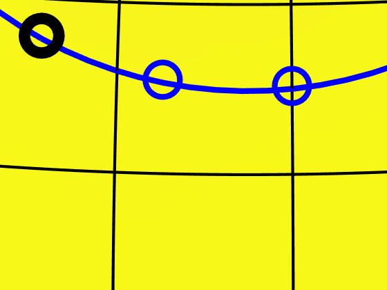
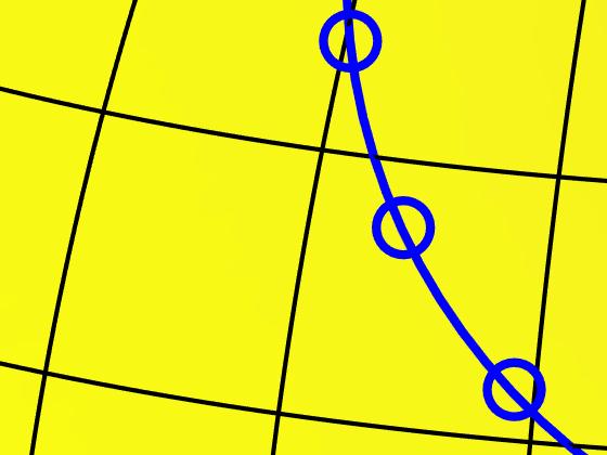
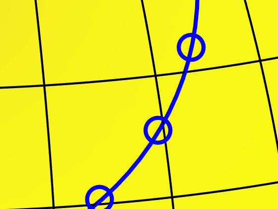
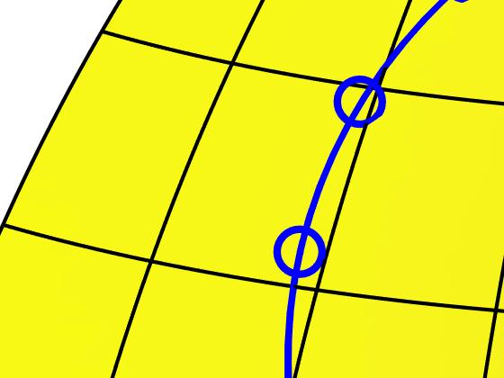
-(c) emerge over time from initial conditions")
 as a function of time τ for five initial")
, which shows the")
. At t = 0, Ṡ() = 0.")

![manifold Θ can then be measured with the statistical distance [44], L = t f](/docs-images/93/118033169/images/3-10.jpg "I F (t).")
 L.")
![(9) Previous work has shown that J L 0 is a temporal variance [7, 8], and](/docs-images/93/118033169/images/3-12.jpg "that, in one representation, can measure cumulative fluctuations in the rate")
![coefficients for irreversible decay processes [45].](/docs-images/93/118033169/images/3-16.jpg "In the current context, the difference between the two terms of the")
 and p(t f ) that measures the cumulative deviations")

![function, A(t), as E[A(t)] = τ 1 t f A(t).](/docs-images/93/118033169/images/3-29.jpg "The difference between the time average of I F and the squared time-average")
![of I F over the path is the time-averaged variance σ = J L τ [ ] = E [I F ]](/docs-images/93/118033169/images/3-31.jpg "E IF 0.")


![These paths correspond to the condition J = L [44] and a variance of zero.](/docs-images/93/118033169/images/3-36.jpg "These certain paths are irreversible, nonstationary paths with zero")


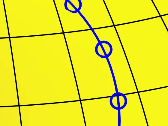
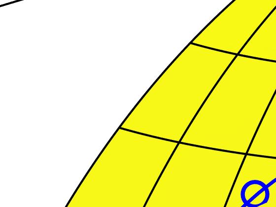
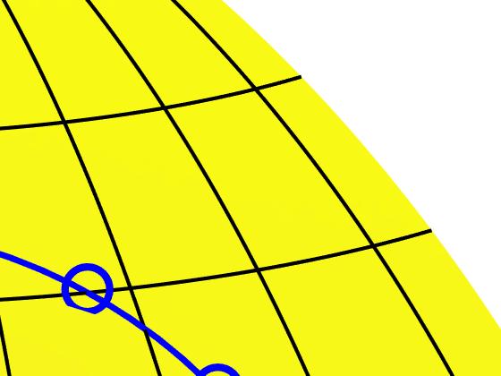
3 3 (a) (b) (c) FIG. 1. Scars on the state space (a)-(c) emerge over time from initial conditions that ultimately dissipate and have higher path uncertainties. The entropy rate Ṡ = Ṡ(t f ) as a function of time τ for five initial conditions equidistant from equilibrium (colors correspond to (b)). The initial conditions are marked by circles in (b), which shows the positive octant of a sphere colored by Ṡ(t f ) when the path reaches the stationary distribution (white square). At t = 0, Ṡ() = 0. (c) The upper bound for Ṡ(t), C σ τ/, for the five select initial conditions as a function of time. manifold Θ can then be measured with the statistical distance [44], L = t f I F (t). The Cauchy-Schwarz inequality yields the statistical divergence, J τ tf I F (t) L. (9) Previous work has shown that J L 0 is a temporal variance [7, 8], and that, in one representation, can measure cumulative fluctuations in the rate coefficients for irreversible decay processes [45]. In the current context, the difference between the two terms of the Cauchy-Schwarz inequality equals the variance or geometric uncertainty of the path connecting p( ) and p(t f ) that measures the cumulative deviations from the geodesic. To illustrate this interpretation, we define the time average for a function, A(t), as E[A(t)] = τ 1 t f A(t). The difference between the time average of I F and the squared time-average of I F over the path is the time-averaged variance σ = J L τ [ ] = E [I F ] E IF 0. (10) This geometric uncertainty is the cumulative deviation from the geodesic connecting the initial and final distributions. It depends on the path and the initial and final distributions. We expect it to be nonzero for most irreversible processes. One notable exception are paths following the geodesic connecting two distributions. These paths correspond to the condition J = L [44] and a variance of zero. These certain paths are irreversible, nonstationary paths with zero geometric uncertainty. It has previously been shown that measuring cumulative deviations from the geodesic amounts to measuring the cumulative fluctuations in nonequilibrium observables [33, 45]. Past work has also used statistical distances (though with other metrics) to measure the dissipation associated with quasistatic transformations [46]. These results, however, do not connect thermodynamic quantities such as the entropic acceleration to the Fisher information for general nonstationary irreversible processes as we do here. Our second main result is a bound on the entropy rate by the geometric uncertainty. It follows from recognizing that the variance satisfies the inequality: σ 1 tf ( [ ] ) I F + E IF J τ τ. (11) The last step uses J L 0 and the nonnegativity of the variance. Defining I τ 1 t f I, this relation becomes I σ 1. (1) The intuition behind this uncertainty relation is that different paths across the manifold of probability distributions Θ can lower the time-averaged rate of information change I, but only at the expense of a corresponding decrease in uncertainty (a smaller excursion from the geodesic). Simply put, the uncertainty places a bound on the cumulative rate of information change. It is worth noting that this information-uncertainty ratio is valid for nonstationary, irreversible paths over any finite time interval between arbitrary probability distributions. To test this inequality, one only needs the basic ingredients of a Markov state model, models that have proven useful for discovering collective variables and analyzing rare events in diverse areas, including protein (un)folding [47, 48]. Another way to write the uncertainty relation is in terms of the entropic acceleration, Eq. (8). Upon integrating, it becomes a bound on the entropy rate Ṡ C σ τ, (13) where, again, C = t f x p x(t) ln p x (t) and Ṡ = Ṡ(t f ) Ṡ(). The quantities C and σ τ/ can both be zero only in a stationary state that is, this uncertainty relation applies specifically to the nonstationary regime
 is bounded by contributions from the local and bulk information dynamics and cumulative deviations")
 flow.")

 becomes τ 1 t f Var [ ɛ(t)] σ /β. The uncertainty measures the cumulative deviations from constant energy rate fluctuations.")
 are")
![constant: I F (t) = β Var [ ɛ(t)] 0. Uncertainty scarring in a single-cycle chemical reaction.](/docs-images/93/118033169/images/4-13.jpg "To illustrate these results, we adapt the kinetic scheme used by Onsager to demonstrate the reciprocal relations of irreversible thermodynamics [49].")
4 4 and are measurable from occupation/transition probabilities. A direct connection to previous stationary uncertainty relations appears to be a subtle question. However, the present result has a clear physical meaning: the entropy rate (from thermodynamics) is bounded by contributions from the local and bulk information dynamics and cumulative deviations from the geodesic (from information geometry). When no heat is exchanged, these information dynamics bound the entropy production. And, when there are no internal sources of entropy production, they bound the entropy (heat) flow. The results so far avoid any assumptions about the probability distributions, rate of driving, or closeness to equilibrium. For additional insight into the bounds placed on energy exchange, consider a system in contact with a heat bath at fixed temperature T, in which the energy of each state of the system is driven slowly. At each moment in time, the probability of state x is p x (t) = e βɛx(t) /Z(t), where ɛ x (t) is the energy of state x and Z(t) is the partition function. Eq. (34) becomes τ 1 t f Var [ ɛ(t)] σ /β. The uncertainty measures the cumulative deviations from constant energy rate fluctuations. The geodesic corresponds to a path where the energy rate fluctuations are time independent. During a nonstationary process operating near this bound, lowering the time-average fluctuations in energy flux will mean smaller excursions from the geodesic where these fluctuations and I F (t) are constant: I F (t) = β Var [ ɛ(t)] 0. Uncertainty scarring in a single-cycle chemical reaction. To illustrate these results, we adapt the kinetic scheme used by Onsager to demonstrate the reciprocal relations of irreversible thermodynamics [49]. The model consists of three states and a kinetics driven by the timedependent rate coefficients, k + = 4 atan(ω 1 t) and k = 4 atan(ω t), with ω 1 = 4 and ω = 6. The inverse tangent function ensures that for large t, every path reaches the same stationary distribution, p x = (1/3, 1/3, 1/3). Our criterion for a path to reach the stationary distribution is that each initial condition must evolve to be within p x (t) p x of the stationary distribution. Under the transformation γ x (t) p x (t), the system travels across the positive octant of a sphere (Fig. (1)). This system and driving protocol localize the effects of the initial condition on the geometric uncertainty about the nonequilibrium path (SM). What we find is that the distance from the stationary state says little about the uncertainty or the entropy rate (dissipation rate). Figure (1b) shows Ṡ = Ṡ(τ) for all physically-relevant initial conditions (color indicates final Ṡ). Five initial conditions are marked (open circles), each point equidistant from the equilibrium state, p x (white square). While these initial conditions are all equally far from equilibrium, their entropy rates exhibit different behavior over time (Figure (1a), color corresponds to those in (b)). Moreover, paths originating on the scar (Fig. (1b)), have a larger maximum value of Ṡ(τ) than those launched FIG.. Accelerating the erasure of information (destroying state x = 0), by increasing ω, generates more (a) uncertainty (σ τ/, dashed lines) about the erasure path and maximum heat dissipated ( q(t), solid lines). (b) The heat dissipated, q(t), follows the geodesic (σ 0) up until the maximum amount of heat is being released. Beyond that point, the system undergoes entropic deceleration. Time series are from p() = [0.5, 0.5] to p(t f ) = [1, 0] for ω = [0.05, 0., 7 = 0.3] shown in blue, black, and red lines, respectively. from off it. These initial conditions are also unique in that they all dissipate for a period of time. Initial conditions off the scar do not dissipate. Regardless of the dissipative nature of these paths, the uncertainty relation holds. The time dependence of the upper bound is shown in Fig. (1c) for the same five initial conditions. Again, those initial conditions originating in the scar have a larger uncertainty and upper bound the entropy rate. Overall, these results are evidence that the distance from the stationary state can be a poor predictor of transient nonequilibrium behavior. Landauer s principle and information erasure. Perhaps nowhere is the connection between information and thermodynamics more apparent than in Landauer s principle [50]. According to this principle, erasing one bit of information requires the dissipation of at least k B T ln thermal energy as heat. Since the bound on Ṡ(t) in Eq. (13), holds for any Markovian evolution between any two distributions, we can explore the connection between the entropy (heat) dissipation and the uncertainty about the erasure path. To examine correlation between erasure paths and the heat release, we consider the erasure of one-bit of information in a model memory device. The model 1-bit memory device initially consists of two states x = {1, 0} that are equally probable, p( ) = [0.5, 0.5]. To measure the heat release, we choose W (t) such that every distribution is of the form p x (t) = Z(t) 1 e βɛx(t), where Z(t) is the partition function, β is the inverse temperature set to one, and ɛ x (t) is the energy at state x (SM). The energy at x = 1, is held fixed and ɛ (t) = c 1 + c /π atan(ωt) depends on ω. Here, c 1 = 0. and c = 0. The parameter ω, controls the rate at k B T ln of energy is dissipated. This restriction on p x (t) means that the entropy rate, Ṡ = x,y W xyp y (ɛ x (t) ɛ y (t)) = q(t), is the average heat exchange between the system and surroundings at an instant in time. From Eq. (13), we know that q(t) C σ τ/. For this sys-
5 5 tem, both C and σ τ/ are positive and q(t) 0, as expected. The higher the rate at which heat is dissipated, the larger the erasure path uncertainty (Fig. (a)). The uncertainty does not increase at a constant rate during the erasure protocol. As energy is initially dissipated, up to the maximum value, the system approximately follows the geodesic across Θ and σ 0. Figure (b) shows σ τ/ is near zero until the system reaches a state of maximal dissipation, after which the path moves off the geodesic. The faster physically-stored information is erased, the faster energy is dissipated and the greater the resulting uncertainty about the path to equilibrium. Conclusions. For processes arbitrarily far from equilibrium, we have established a bound on the entropy production and flow rates via the uncertainty in the path connecting any two arbitrary distributions. This uncertainty relation holds when the system evolves under a time-inhomogeneous Markovian dynamics, making it applicable to a broad class of nonequilibrium processes. It is clear that even for the classical single-cycle system, the proximity to the stationary state is a poor indicator of uncertainty: initial conditions that are statistically equidistant from the stationary state can have dramatically different geometric uncertainties, uncertainties that we showed are linked to the entropy rate. When erasing information in a model one-bit memory device, we find that increasing the speed of erasure comes at the expense of increasing the rate of energy dissipation and the geometric uncertainty about the path to equilibrium. We expect these results to be usefully applied to other kinetic phenomena, such as (bio)chemical reactions [51, 5], and further expand the understanding of processes away from equilibrium, both near and far. Acknowledgments. This material is based upon work supported by the U.S. Army Research Laboratory and the U.S. Army Research Office under grant number W911NF and the John Templeton Foundation. S. B. N. acknowledges financial support from the Office of Global Programs, University of Massachusetts Boston. We thank Sosuke Ito for pointing out the relation between the generalized forces and the matrix E and Tamiki Komatsuzaki for comments on the manuscript. jason.green@umb.edu [1] H. B. Callen, Thermodynamics and an Introduction to Thermostatistics, nd ed. (John Wiley & Sons, Inc., 1985). [] B. Mandelbrot, IRE Transactions on Information Theory, 190 (1956). [3] F. Schlögl, J. Phys. Chem. Solids 49, 679 (1988). [4] J. Uffink and J. van Lith, Found. Phys. 9, 655 (1999). [5] A. C. Barato and U. Seifert, Phys. Rev. Lett. 114, (015). [6] T. R. Gingrich, J. Horowitz, N. Perunov, and J. England, Phys. Rev. Lett. 116, (016). [7] C. Maes, Physical review letters 119, (017). [8] J. M. Horowitz and T. R. Gingrich, Phys. Rev. E 96, (017). [9] P. Pietzonka, F. Ritort, and U. Seifert, arxiv: (017). [10] N. Shiraishi, K. Saito, and H. Tasaki, Phys. Rev. Lett. 117, (016). [11] N. Shiraishi, arxiv: (017). [1] K. Proesmans and C. Van den Broeck, EPL 119, 0001 (017). [13] A. Dechant and S. Sasa, arxiv: (017). [14] C. Jarzynski, Phys. Rev. Lett. 78, 690 (1997). [15] U. Seifert, Rep. Prog. Phys. 75, (01). [16] R. Kawai, J. M. R. Parrondo, and C. Van den Broeck, Phys. Rev. Lett. 98, (007). [17] D. J. A. E. Allahverdyan and G. Mahler, J. Stat. Mech. 009, P09011 (009). [18] D. Hartich, A. Barato, and U. Seifert, J. Stat. Mech. 014, P0016 (014). [19] J. M. Horowitz and M. Esposito, Phys. Rev. X 4, (014). [0] S. Yamamoto, S. Ito, N. Shiraishi, and T. Sagawa, Phys. Rev. E 94, 0511 (016). [1] J. M. R. Parrondo, J. M. Horowitz, and T. Sagawa, Nat. Phys. 11, 131 (015). [] S. Lloyd, Nature 406, 1047 (000). [3] A. B. Boyd and D. M. J. P. Crutchfield, New J. Phys. 18, (016). [4] T. M. Cover and J. A. Thomas, Elements of Information theory, nd ed. (Wiley, 006). [5] S. Amari and H. Nagaoka, Methods of information geometry, Vol. 191 (American Mathematical Soc., 007). [6] D. Brody and N. Rivier, Phys. Rev. E 51, 1006 (1995). [7] J. Heseltine and E. Kim, J. Phys. A 49, (016). [8] S. B. Nicholson and E. Kim, Entropy 18, 58 (016). [9] M. Oizumi, N. Tsuchiya, and S. Amari, Proc. Natl. Acad. Sci. U.S.A. 113, (016). [30] F. Weinhold, J. Chem. Phys. 63, 479 (1975). [31] G. E. Crooks, Phys. Rev. Lett. 99, (007). [3] G. Ruppeiner, Phys. Rev. A. 0, 1608 (1979). [33] D. A. Sivak and G. E. Crooks, Phys. Rev. Lett. 108, (01). [34] S. Lahiri, J. Sohl-Dickstein, and S. Ganguli, arxiv: (016). [35] J. Schnakenberg, Rev. Mod. Phys. 48, 571 (1976). [36] R. C. Rao, J. Royal Statistics Society B10, 159 (1945). [37] R. A. Horn and C. R. Johnson, Matrix Analysis (Cambridge university press, 01). [38] S. B. Nicholson, L. S. Schulman, and E. Kim, Phys. Lett. A 377, 1810 (013). [39] S. B. Nicholson and E. Kim, Physica Scripta 91, (016). [40] B. R. Frieden, Science from Fisher Information, Vol. (Cambridge University Press, 004). [41] C. E. Shannon, The Bell System Technical Journal 7, 63 (1948). [4] M. Esposito and C. Van den Broeck, Phys. Rev. E 8, (010). [43] U. Seifert, Phys. Rev. Lett. 95, (005). [44] W. K. Wootters, Phys. Rev. D 3, 357 (1981). [45] S. W. Flynn, H. C. Zhao, and J. R. Green, J. Chem. Phys. 141, (014); J. W. Nichols, S. W. Flynn, and J. R. Green, ibid. 14, (015). [46] P. Salamon and R. S. Berry, Phys. Rev. Lett. 51 (1983).
6 6 [47] C.-B. Li and T. Komatsuzaki, Phys. Rev. Lett. 111, (013). [48] B. E. Husic and V. S. Pande, J. Am. Chem. Soc. 140, 386 (018). [49] L. Onsager, Phys. Rev. 37, 405 (1931). [50] R. Landauer, IBM J. Res. Dev. 5, 183 (1961). [51] A. C. Barato, D. Hartich, and U. Seifert, New J. Phys. 16, (014). [5] T. McGrath, N. S. Jones, P. R. ten Wolde, and T. E. Ouldridge, Phys. Rev. Lett. 118, (017). [53] J. Norris, Markov Chains, Vol. 1st (Cambridge University Press, 1997). [54] G. E. Crooks, Fisher information and statistical mechanics, Tech. Rep. (Citeseer, 011). [55] Though starting from different initial conditions, q() = [0.5539, , 0.677], q() = [0.513, , ], both regions have equal uncertainty at t = and (numerically) equivalent values of σ and I at all times. SUPPLEMENTAL INFORMATION PROPERTIES OF THE MATRIX, E In this section, we will derive properties of the matrix, E xy (t) = W xy (t) C xy(t), (14) that underlie the results in the main text. We will use bra and ket notation, so that given the N N matrix, E, we have [E p ] x = y E xyp y and [ p E] y = x p xe xy. I. Master equation. The master equation can be recast in terms of the matrix E(t). Multiplying E(t) by the probability and summing gives, E xy (t) = ( W xy (t) C ) xy(t), p y y y (t) E xy (t) = ṗ x (t) ṗx(t), y y E xy (t) = ṗ x (t) = y W xy (t). (15) The final line shows that E(t) is an alternative representation of the dynamics governed by the master equation. We should note that E(t) is not a trivial transformation of W (t). For example, E(t) W (t). Instead, multiplying E(t) by two, shows that if C xy (t) = 0 x, y then E(t) = W (t). In general, however, E xy (t) = W xy (t)+ŵxy(t), where Ŵxy(t) is the time-reversed rates defined [53] by Ŵ xy (t) = W yx (t)p x (t), Ŵ xy (t) = 1 W yx(t)p x (t). (16) The matrix Ŵ (t) defines the microscopically reverse dynamics of W xy (t), which do not satisfy detailed balance in general. In fact, only when W (t) satisfies detailed balance, does W xy (t) = Ŵxy(t). II. Detailed balance condition. The rate matrix has the properties that W xy (t) W(t), W xy (t) > 0 for x y and W yy (t) = x y W xy(t) so that x W xy(t) = 0. Using the last property, the master equation becomes ṗ x (t) = y x = y [W xy (t) W yx (t)p x (t)] C xy (t). (17) The master equation exhibits detailed balance if each of the currents vanish; that is, when the currents or thermodynamic fluxes, C xy (t) = W xy (t) W yx (t)p x (t), are zero for all x, y. Otherwise, the existence of current implies the system is undergoing an irreversible process [35]. Even for processes that are driven or transiently away from equilibrium, C xy (t) 0, the matrix E(t) satisfies a similar detailed balance condition. Since the master equation can be recast in terms of E(t), it also has an analogous form with source and sink terms. Applying the definition of E(t) to the master equation gives ṗ x (t) = [E xy (t) E yx (t)p x (t) + C xy (t)] y x = [ C E xy (t) + C xy (t) ]. (18) y In the final line, we define the current (for E(t)) between states x and y, C E xy(t). Comparing this result to Eq. (17) suggests C E xy(t) = 0, akin to detailed balance, but valid when C xy (t) 0. To prove this detailed balance condition, we can expand the current for E(t): C E xy(t) E xy (t) E yx (t)p x (t) = W xy (t) C xy(t) = C xy(t) + C yx(t) W yx (t)p x (t) + C yx(t) = 0. (19) The last equality follows from the anti-symmetry of the current, C xy (t) = C yx (t). When detailed balance is satisfied for C xy (t) it is also satisfied for Cxy(t): E the condition for both is W xy (t) = W yx (t)p x (t). III. Symmetrization. As is done at equilibrium with W (t), we can show that E(t) is similar to a symmetric matrix, S(t): E(t) S(t). First, we define S xy (t) = 1 px (t) E xy(t). (0)
7 7 To show S(t) is symmetric, we use S(t) and the detailed balance of E(t): E xy (t) = E yx (t)p x (t), px (t)s xy (t) = S yx (t) p x (t), S yx (t) = S xy (t). (1) Since S(t) is a real, symmetric (Hermitian) matrix, it has a complete set of eigenvectors and real eigenvalues [37]. Since E(t) is similar to S(t), it also has a complete set of eigenvectors and real eigenvalues. We note that the eigenvectors and eigenvalues of both matrices are time dependent. The E-representation of the master equation, Eq. (15), does not imply that W (t) is similar to S(t). From the definitions of E(t) and S(t), Eq. (14) and Eq. (0), we know E xy (t) = 1 p x (t)s xy (t) py (t). Re-writing in terms of S(t) gives: S xy (t) = 1 px (t) W C xy (t) xy(t) p x (t). By inspection, W (t) is only similar to S(t) when C xy (t) = 0 x, y and E(t) = W (t). It can be further shown that just because E(t) S(t) through p x (t), this does not imply S (t) W (t), where S xy(t) = S yx(t). Defining S (t) as S xy(t) = 1 px (t) W xy(t). and using the expression for the current, C xy (t) = W xy (t) W yx (t)p x (t) = p x (t)s xy(t) p x (t) S yx(t) p x (t), yields S xy(t) = C xy (t) px (t) + S yx(t). Thus, S (t) cannot be symmetric unless the detailed balance is satisfied, C(t) = 0, or S is the zero matrix. It is the nonstationary, irreversibility of the system that prevents W (t) from satisfying a similarity transform irreversibility is built into E(t). IV. Surprisal rate. Shannon [41] identified the information gained or surprise in observing the state y as ln [4]. Using x E xy(t) = [ 1 E(t)] y, where 1 is a row vector of ones, the surprisal rate is related to E by [ 1 E(t)] y = x [ W xy (t) C ] xy(t) = ṗy(t) = 1 d ln. () This relationship also implies, through conservation of probability, that E(t) p(t) = y ṗy(t) = 0. V. Fisher information. Underlying the principal results of the main text is that E(t) is related to the Fisher information, I F (t), through I F (t) = Ė(t) p(t) = E(t) ṗ(t). Differentiating E(t) p(t) with respect to time gives d E(t) p(t) = E(t) ṗ(t) + Ė(t) p(t). (3) The first term on the right-hand side is the Fisher information, E(t) ṗ(t) = ( W xy (t)ṗ y (t) C ) xy(t)ṗ y (t) p x,y y (t) = x,y = y 1 C yx(t)ṗ y (t) ṗ y (t) = I F (t). (4) The second term is the negative of the Fisher information: Ė(t) p(t) = xy = x,y = x,y (Ẇxy (t) + C xy(t)ṗ y (t) C xy (t)ṗ y (t) C yx (t)ṗ y (t) ) Ċxy(t) = I F (t). (5) From the first to the second line, we use conservation of probability, d/ x W xy(t) = 0, and d/ xy C xy(t) = 0. Plugging Eq. (4) and Eq. (5) into Eq. (3), we see that the conservation of probability leads to d E(t) p(t) = I F (t) I F (t) = 0. VI. Fisher information as entropic acceleration. With the properties discussed so far, we can arrive at the first main result: for systems with dynamics that are governed by continuous-time master equations, the Fisher
8 8 information is part of the entropic acceleration. To show this, we recognize that the matrix E(t) in Property IV can be expressed in terms of the generalized thermodynamic forces, [ E(t) ] y = 1 = 1 = 1 = x C yx (t) x W yx (t)p x (t) W xy (t) x x ( ) Wyx (t)p x (t) W xy (t) W xy (t) 1 W xy (t)e Fxy(t), (6) where F xy (t) = ln W xy (t) ln W yx (t)p x (t). In Property V, we proved that I F = Ė(t) p(t). Using this relation, together with the definition of the thermodynamic forces, shows the Fisher information is given by I F (t) = Ė(t) p(t) = [ d ( W xy (t)e Fxy(t))] x,y = (Ẇxy (t)e Fxy(t) x,y W xy (t) F ) xy (t)e Fxy(t) = x,y W xy (t) d ln ( py (t) p x (t) = I(t). (7) Since ln is the surprisal of state y at time t, the quantity I(t) is the time rate of change in the surprisal difference (between y and x). To connect I F (t) to the entropic acceleration, we differentiate the entropy rate, Ṡ(t) = [ ] py (t) W xy (t) ln, (8) p x,y x (t) with respect to time: S(t) = d [W xy(t)] I xy W xy (t) I xy (t) x,y x,y = d [W xy(t)] I xy (t) I F (t) x,y = x p x (t) ln p x (t) I F (t), (9) where I xy = ln + ln p x (t). From Eq. (7), the second term in the entropic acceleration is minus the Fisher information. The entropy rate Ṡ(t) is an average over the change in information I(t), so S(t) can be thought of as the rate of change of the bulk, or average information, ) S(t) = d I(t) /. The Fisher information, though, is an average over the rate of change in information between each set of states x and y, I F = I(t). Therefore, the first term on the right hand side of Eq. (9) is the sum of the bulk information rate and the average local information rate, x p x (t) ln p x (t) = S + I F = d I(t) + SPECIAL CASES di(t). (30) An intuitive physical interpretation of the results in the main text is acquired by considering several special cases. The Fisher information is I F I = x,y W xy p y Ixy = S i + S e. (31) It is important to note that the angled brackets on the outside of the time derivative refer to the average over the local change, instead of the change in the average quantity, i.e., Si S i, in general. The average entropic accelerations S i and S e are defined as and S i = x,y S e = x,y W xy (t) d ln ( Wxy (t) W yx (t)p x (t) ) (3) W xy (t) d ( ) ln Wxy (t). (33) W yx (t) The uncertainty relation can be written as tf tf [ I F = S i + S ] e σ τ. (34) Steady-states. In a steady state, ṗ x = 0 and the Fisher information is I F = 0. As a consequence, there is zero path uncertainty σ = I = 0. From Eq. (31), this means that the local entropy production rate and entropy flow rate are exactly in balance: S i = F = S e. Geodesic. If the average local rate of information change is constant, (i.e., the path is certain): I = I = S i + S e (geodesic). (35) The average local entropic acceleration is constant, independent of time and distance from the final distribution. Zero entropy flow. If the entropy flow is zero, say, when the system is connected to an idealized bath [4], then the uncertainty principle becomes τ 1 tf S i σ. (36)
9 9 Zero entropy production. If the entropy production is zero, then the uncertainty principle becomes τ 1 tf S e σ. (37) Exponential probability distributions. While the above results are independent of the form of the probability distributions, the special case of an exponential energy distribution gives further physical insight. Of particular interest is a single-component, homogeneous, closed system at thermal equilibrium with a reservoir at inverse temperature β = 1/k B T : p x (t) = Z 1 e βɛx(t). (38) Using the detailed balance condition (Property II above), which holds regardless of the distribution, the probability of state y relative to state x is p x (t) = E yx(t) E xy (t) = e β[ɛy(t) ɛx(t)] = e βqyx(t). (39) We define the energy exchanged as heat during the transition from x to y as q yx = ɛ y (t) ɛ x (t). With this definition, the Fisher equation and the heat are directly related, I F (t) = β q(t) xy = xy = β ɛ(t) = xy W xy (t) q xy (t) W xy (t) ɛ x (t). (40) As a result, the Fisher information is the rate at which energy flows into the system as heat, scaled by the temperature of the reservoir. The time average of this quantity appears in the uncertainty principle, the second main result in the paper. For a system evolving along the geodesic, β q(t) xy is independent of time: energy is exchanged between the system and reservoir as heat at a constant rate. For this special case, we have the Shannon information, S(t) = x the entropy rate, Ṡ(t) = xy p x (t) ln p x (t) = β ɛ(t), (41) W xy (t) ln p y(t) p x (t) = β q(t) xy, (4) and the entropic acceleration, S(t) = β d q(t) xy = β d dq(t) [W xy(t)] q xy (t) + β x xy = β dq(t) p x (t)ɛ x (t) + β. (43) x xy We now drop the subscript xy on the average. Integrating from an initial time,, to a final time, t f, shows that over any arbitrary interval of time, q(t) t tf f = x tf p x (t)ɛ x (t) + q(t), (44) there are two contributions to the energy exchanged as heat. We note that if the heat flow is constant, as in a nonequilibrium steady-state, or zero, as in an equilibrium state, then both sides of this equality must vanish. Also, we can recognize the second term as the time-integrated (necessarily positive) Fisher information up to a factor of β. In this case, the first inequality in the main text is Using this inequality, we get β tf q(t) σ τ. (45) q(t) t tf f x p x (t)ɛ x (t) σ τ β. (46) Energy fluctuations. Crooks, [54] showed that for a canonical ensemble, the Fisher information is equal to the infinitesimal change in energy with respect to a change in the control parameter, ( ɛ I F (θ) = β ɛ ). (47) θ θ If β is the control parameter, this expression becomes the variance measuring energy fluctuations around equilibrium. Here, we derive a similar result. We will also assume that our distributions are exponential, but that the control parameter (here, time) is varied smoothly and arbitrarily. The distributions are then time dependent and β is fixed. In this case, I F measures the fluctuations in the energy rates. Given p x (t) = Z(t) 1 exp( βɛ x (t)), the change in probability is, ṗ x (t) = β ɛ x (t)p x (t) p x (t)ż Z = β ɛ x (t)p x (t) + βp x (t) x ɛ x (t)p x (t). (48) Writing the ensemble average as x p x(t)[ ] =, d ln p x(t) = β ɛ(t) β ɛ x (t), ( ) d ln px (t) = β( ɛ x (t) ɛ(t) ), ( ) d ln px (t) p x (t) = β Var[ ɛ(t)], x I F (t) = β Var[ ɛ(t)]. (49)


 The uncertainty and cumulative rate of information change")

.")


] t0 σ.")


 = [1, 0] at the final time.")

, where Z(t) is the partition function, β is the inverse")


10 10 (a) (b) (c) (d) <, I <, I t t FIG. 3. Scars on the state space (a)-(c) appear over time from either higher information rates or low path uncertainties. (a) Initially, all initial conditions have a low ratio of the cumulative rate of information change, I, and uncertainty, σ. (b) At intermediate times, different initial conditions have a drastically different value of I/σ. (c) At long times, slow initial conditions are washed out by time averaging but those scarring the state space reach the stationary state (open circle) quickly. (d) The uncertainty and cumulative rate of information change for four representative initial conditions. Green and blue lines are initial conditions an equal distance from the stationary state (colored according to the value of I/σ ). Yellow lines correspond to the bright I/σ regions in (c). In this case, the energy is playing the role of our control parameter and β is held fixed, so the Fisher information measures the fluctuations in the energy rate. Using the first inequality from the main text gives, β τ Z tf Var[ (t)] t0 σ. (50) The uncertainty over the path lower bounds timeaveraged fluctuations of the energy rates. The geodesic is a path traversed when systems have no fluctuations in the energy rate. All other paths will have a positive variance. MODELS Landauer principle. Consider a system initially exchanging energy with the reservoir at inverse temperature β and relaxing to thermal equilibrium. The two states x = {1, 0} are observed with probability px (t0 ) = [.5,.5] initially and px (tf ) = [1, 0] at the final time. The net result is the erasure of state x = 0. So that the heat can be measured during this evolution, we choose a driving protocol such that px (t) = Z(t) 1 e β x (t), where Z(t) is the partition function, β is the inverse temperature of the bath, and x (t) is the energy at state x. To ensure that our dynamics generates the prescribed sequence of distributions, we work backwards. Given px (t) for t0 t tf, we estimate p x (t) = [px (t + δt) px (t)]/δt, where δt = was used for all simulations. To find the W (t) that satisfies W (t) p(t)i = p (t)i, we solve the system of linear equations using conservation of probability, W11 (t) = W1 (t), W (t) = W1 (t). There is an infinite family of W (t) that satisfies these conditions given by, " # 1 (t) A p 1 (t)+ap p (t) W (t) =. (51) 1 (t) A p 1 (t)+ap p (t) We set A, which is arbitrary, to one. To calculate the second P inequality in the main text, we need to evaluate x p x (t) ln px (t). Given px (t) = Z(t) 1 e β x (t), the first and second derivatives give, p x (t) = βpx (t) ( (t)p (t) x (t)). (5) p x (t) =β p x (t) [ (t)p (t) x (t)] + + βpx (t) [ (t)p (t) + (t)p (t) x (t)]. (53) For the energies, we hold 1 (t) = (t0 ) constant, making our initial distribution px (t0 ) = [0.5, 0.5], and vary (t) = c1 + cπ atan(ωt), where we use c1 = 0., and c = 0. The first and second derivatives for px (t) are then (t) = 0ω, π[1 + ω t ] (54) (t) = 40ω 3 t. π[1 + ω t ] (55) FIG. 4. The maximum instantaneous average heat and maximum uncertainty grow linearly with increasing driving rate, ω. The coefficients for max hhq(t)ii = a1 ω + a are, a1 = 1.349, a = , while for max[σ τ /] they are a1 = and a = 0.0.
 symmetry and (b) broken symmetry.")
 and max[σ τ/] increase linearly with ω. For 0 evenly spaced values of ω, ranging from 0.05 to 1.")
 k t +.")
.")
.")
![One prominent feature is the two (yellow, [55]) regions of initial conditions that have a large ratio relative to the rest of the state space.](/docs-images/93/118033169/images/11-8.jpg "The time series of these initial conditions are shown in Fig. (3d) (yellow), where we see that it is predominately the small uncertainty that is generating the large ratio.")

![(3d) shows the time series for one of these initial conditions (green solid/dashed lines q( ) = [0.6491, 0.5796, 0.497]). To contrast paths originating from the scar, the blue line in Fig.](/docs-images/93/118033169/images/11-10.jpg "(3d) corresponds to an initial condition (q( ) = [0.4953, 0.5751, 0.6511]) that is equidistant from p but lies outside the scar.")


11 11 (a) 1 k + (t) k (t) k + (t) k (t) 3 k + (t) k (t) (b) 1 k (t) k (t) k + (t) k + (t) 3 k (t) k + (t) FIG. 5. Kinetic scheme for a driven version of Onsager s three-state model with (a) symmetry and (b) broken symmetry. In the main text, we describe how the system initially follows the geodesic and only deviates after the maximum heat has been dissipated. We also find for this system that both max q(t) and max[σ τ/] increase linearly with ω. For 0 evenly spaced values of ω, ranging from 0.05 to 1.1 we evolve each for the same time, and record the maximum value of q(t) and σ τ/. These quantities are shown in Fig. (4), with the maximum heat in red and maximum uncertainty in black. Driven versions of Onsager s three-state model For the three state model in the manuscript, the rate matrix takes the form: kt k t + k + t W = kt (kt + k t + ) k t +. kt kt k t + The k + t rate is given by k + t = 4 π atan(ω+ t) and the k t rate is k t = 4 π atan(ω t) as shown in Fig. (6). To test the uncertainty relation, we calculate the ratio, I/σ to confirm that it is larger than 1/, Fig. (3a-c). Each initial condition starts with roughly the same ratio of information to uncertainty, Fig. (3a). Because the rate of information change and the variance are path dependent, the dynamics quickly generate a wide range of ratios, Fig. (3b). One prominent feature is the two (yellow, [55]) regions of initial conditions that have a large ratio relative to the rest of the state space. The time series of these initial conditions are shown in Fig. (3d) (yellow), where we see that it is predominately the small uncertainty that is generating the large ratio. We also see that this large ratio disappears as the path approaches p. Fig. (3c) shows the ratio for the (minimum) time it takes for all initial conditions to become within of p. Also prominent is a scar where initial conditions quickly close in on p at the cost of high cumulative entropic accelerations/change in information. Fig. (3d) shows the time series for one of these initial conditions (green solid/dashed lines q( ) = [0.6491, , 0.497]). To contrast paths originating from the scar, the blue line in Fig. (3d) corresponds to an initial condition (q( ) = [0.4953, , ]) that is equidistant from p but lies outside the scar. The path followed from this starting point has a lower σ and I, showing that the shortest distance from the stationary point is a poor indicator of the behavior of the process. In the main text, we analyze a driven three state model with broken symmetry. For comparison, we show the symmetric driven Onsager model. The same driving protocol is used but the rate matrix is (kt + k t + ) kt k + t W = k t + (kt + k t + ) kt. kt k t + (kt + k t + ) FIG. 6. Rate coefficients for different values of the driving rate ω. The lines in blue and red correspond to ω = 4 and ω = 6, respectively, used in the three state model. As we see, increasing ω increases the rate that k approaches a limiting value. In this model, every initial condition reaches the same stationary state p = [1/3, 1/3, 1/3]. There is a forward cycle and a reverse cycle. We see in Fig. (7) that there is no scarring from high entropy rate initial conditions. Now every initial condition reaches approximately the same final entropy rate in the same time τ. Initial conditions an equal distance from the stationary point seem to have nearly equivalent time evolutions, varying only slightly in the final, maximum value of Ṡ(τ) reached. The upper bound (on Ṡ(τ)) also has nearly the same temporal behavior, regardless of initial condition. It appears that the breaking of the symmetry in the rate matrix leads to the scarring of state space and possibility of dissipative initial conditions.
 FIG.")


12 1 (a) (b) (c) FIG. 7. Lack of state-space scarring in the symmetric, driven Onsager model. (b) Each point on the octant of the sphere is an initial condition that we evolve to the stationary distribution p = [1/3, 1/3, 1/3]. Unlike the asymmetric case, each initial condition generates the same final value of Ṡ(τ). (a) The entropy rate Ṡ(τ) for the set of conditions specifed by the blue circles. (c) The upper bound of these points, all of which evolve similarly in time.
J. Stat. Mech. (2011) P07008
 P07008") Journal of Statistical Mechanics: Theory and Experiment On thermodynamic and microscopic reversibility Gavin E Crooks Physical Biosciences Division, Lawrence Berkeley National Laboratory, Berkeley, CA
Journal of Statistical Mechanics: Theory and Experiment On thermodynamic and microscopic reversibility Gavin E Crooks Physical Biosciences Division, Lawrence Berkeley National Laboratory, Berkeley, CA
Maxwell's Demon in Biochemical Signal Transduction
 Maxwell's Demon in Biochemical Signal Transduction Takahiro Sagawa Department of Applied Physics, University of Tokyo New Frontiers in Non-equilibrium Physics 2015 28 July 2015, YITP, Kyoto Collaborators
Thermodynamic Computing. Forward Through Backwards Time by RocketBoom
 Thermodynamic Computing 1 14 Forward Through Backwards Time by RocketBoom The 2nd Law of Thermodynamics Clausius inequality (1865) S total 0 Total Entropy increases as time progresses Cycles of time R.Penrose
Thermodynamics for small devices: From fluctuation relations to stochastic efficiencies. Massimiliano Esposito
 Thermodynamics for small devices: From fluctuation relations to stochastic efficiencies Massimiliano Esposito Beijing, August 15, 2016 Introduction Thermodynamics in the 19th century: Thermodynamics in
Introduction to Stochastic Thermodynamics: Application to Thermo- and Photo-electricity in small devices
 Université Libre de Bruxelles Center for Nonlinear Phenomena and Complex Systems Introduction to Stochastic Thermodynamics: Application to Thermo- and Photo-electricity in small devices Massimiliano Esposito
arxiv: v2 [cond-mat.stat-mech] 16 Mar 2012
![arxiv: v2 [cond-mat.stat-mech] 16 Mar 2012](/thumbs/73/68169064.jpg "arxiv: v2 [cond-mat.stat-mech] 16 Mar 2012") arxiv:119.658v2 cond-mat.stat-mech] 16 Mar 212 Fluctuation theorems in presence of information gain and feedback Sourabh Lahiri 1, Shubhashis Rana 2 and A. M. Jayannavar 3 Institute of Physics, Bhubaneswar
arxiv:119.658v2 cond-mat.stat-mech] 16 Mar 212 Fluctuation theorems in presence of information gain and feedback Sourabh Lahiri 1, Shubhashis Rana 2 and A. M. Jayannavar 3 Institute of Physics, Bhubaneswar
Nonequilibrium Thermodynamics of Small Systems: Classical and Quantum Aspects. Massimiliano Esposito
 Nonequilibrium Thermodynamics of Small Systems: Classical and Quantum Aspects Massimiliano Esposito Paris May 9-11, 2017 Introduction Thermodynamics in the 19th century: Thermodynamics in the 21th century:
arxiv: v2 [cond-mat.stat-mech] 3 Jun 2018
![arxiv: v2 [cond-mat.stat-mech] 3 Jun 2018](/thumbs/85/91859417.jpg "arxiv: v2 [cond-mat.stat-mech] 3 Jun 2018") Marginal and Conditional Second Laws of Thermodynamics Gavin E. Crooks 1 and Susanne Still 2 1 Theoretical Institute for Theoretical Science 2 University of Hawai i at Mānoa Department of Information and
Marginal and Conditional Second Laws of Thermodynamics Gavin E. Crooks 1 and Susanne Still 2 1 Theoretical Institute for Theoretical Science 2 University of Hawai i at Mānoa Department of Information and
Second law, entropy production, and reversibility in thermodynamics of information
 Second law, entropy production, and reversibility in thermodynamics of information Takahiro Sagawa arxiv:1712.06858v1 [cond-mat.stat-mech] 19 Dec 2017 Abstract We present a pedagogical review of the fundamental
Entropy production fluctuation theorem and the nonequilibrium work relation for free energy differences
 PHYSICAL REVIEW E VOLUME 60, NUMBER 3 SEPTEMBER 1999 Entropy production fluctuation theorem and the nonequilibrium work relation for free energy differences Gavin E. Crooks* Department of Chemistry, University
Beyond the Second Law of Thermodynamics
 Beyond the Second Law of Thermodynamics C. Van den Broeck R. Kawai J. M. R. Parrondo Colloquium at University of Alabama, September 9, 2007 The Second Law of Thermodynamics There exists no thermodynamic
arxiv: v1 [cond-mat.stat-mech] 6 Mar 2008
![arxiv: v1 [cond-mat.stat-mech] 6 Mar 2008](/thumbs/86/93817801.jpg "arxiv: v1 [cond-mat.stat-mech] 6 Mar 2008") CD2dBS-v2 Convergence dynamics of 2-dimensional isotropic and anisotropic Bak-Sneppen models Burhan Bakar and Ugur Tirnakli Department of Physics, Faculty of Science, Ege University, 35100 Izmir, Turkey
CD2dBS-v2 Convergence dynamics of 2-dimensional isotropic and anisotropic Bak-Sneppen models Burhan Bakar and Ugur Tirnakli Department of Physics, Faculty of Science, Ege University, 35100 Izmir, Turkey
The physics of information: from Maxwell s demon to Landauer. Eric Lutz University of Erlangen-Nürnberg
 The physics of information: from Maxwell s demon to Landauer Eric Lutz University of Erlangen-Nürnberg Outline 1 Information and physics Information gain: Maxwell and Szilard Information erasure: Landauer
PHYS 414 Problem Set 4: Demonic refrigerators and eternal sunshine
 PHYS 414 Problem Set 4: Demonic refrigerators and eternal sunshine In a famous thought experiment discussing the second law of thermodynamics, James Clerk Maxwell imagined an intelligent being (a demon
Efficiency at Maximum Power in Weak Dissipation Regimes
 Efficiency at Maximum Power in Weak Dissipation Regimes R. Kawai University of Alabama at Birmingham M. Esposito (Brussels) C. Van den Broeck (Hasselt) Delmenhorst, Germany (October 10-13, 2010) Contents
Emergent Fluctuation Theorem for Pure Quantum States
 Emergent Fluctuation Theorem for Pure Quantum States Takahiro Sagawa Department of Applied Physics, The University of Tokyo 16 June 2016, YITP, Kyoto YKIS2016: Quantum Matter, Spacetime and Information
PHYSICS 715 COURSE NOTES WEEK 1
 PHYSICS 715 COURSE NOTES WEEK 1 1 Thermodynamics 1.1 Introduction When we start to study physics, we learn about particle motion. First one particle, then two. It is dismaying to learn that the motion
Quantum Mechanical Foundations of Causal Entropic Forces
 Quantum Mechanical Foundations of Causal Entropic Forces Swapnil Shah North Carolina State University, USA snshah4@ncsu.edu Abstract. The theory of Causal Entropic Forces was introduced to explain the
Fluctuation theorems. Proseminar in theoretical physics Vincent Beaud ETH Zürich May 11th 2009
 Fluctuation theorems Proseminar in theoretical physics Vincent Beaud ETH Zürich May 11th 2009 Outline Introduction Equilibrium systems Theoretical background Non-equilibrium systems Fluctuations and small
Mathematical Structures of Statistical Mechanics: from equilibrium to nonequilibrium and beyond Hao Ge
 Mathematical Structures of Statistical Mechanics: from equilibrium to nonequilibrium and beyond Hao Ge Beijing International Center for Mathematical Research and Biodynamic Optical Imaging Center Peking
arxiv: v2 [cond-mat.stat-mech] 26 Jan 2012
![arxiv: v2 [cond-mat.stat-mech] 26 Jan 2012](/thumbs/84/89133496.jpg "arxiv: v2 [cond-mat.stat-mech] 26 Jan 2012") epl draft Efficiency at maximum power of minimally nonlinear irreversible heat engines arxiv:1104.154v [cond-mat.stat-mech] 6 Jan 01 Y. Izumida and K. Okuda Division of Physics, Hokkaido University - Sapporo,
epl draft Efficiency at maximum power of minimally nonlinear irreversible heat engines arxiv:1104.154v [cond-mat.stat-mech] 6 Jan 01 Y. Izumida and K. Okuda Division of Physics, Hokkaido University - Sapporo,
Nonequilibrium thermodynamics at the microscale
 Nonequilibrium thermodynamics at the microscale Christopher Jarzynski Department of Chemistry and Biochemistry and Institute for Physical Science and Technology ~1 m ~20 nm Work and free energy: a macroscopic
Information Landscape and Flux, Mutual Information Rate Decomposition and Connections to Entropy Production
 entropy Article Information Landscape and Flux, Mutual Information Rate Decomposition and Connections to Entropy Production Qian Zeng and Jin Wang,2, * State Key Laboratory of Electroanalytical Chemistry,
Information Thermodynamics on Causal Networks
 1/39 Information Thermodynamics on Causal Networks FSPIP 2013, July 12 2013. Sosuke Ito Dept. of Phys., the Univ. of Tokyo (In collaboration with T. Sagawa) ariv:1306.2756 The second law of thermodynamics
Hardwiring Maxwell s Demon Tobias Brandes (Institut für Theoretische Physik, TU Berlin)
") Hardwiring Maxwell s Demon Tobias Brandes (Institut für Theoretische Physik, TU Berlin) Introduction. Feedback loops in transport by hand. by hardwiring : thermoelectric device. Maxwell demon limit. Co-workers:
Hardwiring Maxwell s Demon Tobias Brandes (Institut für Theoretische Physik, TU Berlin) Introduction. Feedback loops in transport by hand. by hardwiring : thermoelectric device. Maxwell demon limit. Co-workers:
Introduction to Fluctuation Theorems
 Hyunggyu Park Introduction to Fluctuation Theorems 1. Nonequilibrium processes 2. Brief History of Fluctuation theorems 3. Jarzynski equality & Crooks FT 4. Experiments 5. Probability theory viewpoint
On the Asymptotic Convergence. of the Transient and Steady State Fluctuation Theorems. Gary Ayton and Denis J. Evans. Research School Of Chemistry
 1 On the Asymptotic Convergence of the Transient and Steady State Fluctuation Theorems. Gary Ayton and Denis J. Evans Research School Of Chemistry Australian National University Canberra, ACT 0200 Australia
Optimal quantum driving of a thermal machine
 Optimal quantum driving of a thermal machine Andrea Mari Vasco Cavina Vittorio Giovannetti Alberto Carlini Workshop on Quantum Science and Quantum Technologies ICTP, Trieste, 12-09-2017 Outline 1. Slow
arxiv: v1 [cond-mat.stat-mech] 28 Sep 2017
![arxiv: v1 [cond-mat.stat-mech] 28 Sep 2017](/thumbs/94/118066307.jpg "arxiv: v1 [cond-mat.stat-mech] 28 Sep 2017") Stochastic thermodynamics for a periodically driven single-particle pump Alexandre Rosas Departamento de Física, CCEN, Universidade Federal da Paraíba, Caixa Postal 58, 5859-9, João Pessoa, Brazil. Christian
Stochastic thermodynamics for a periodically driven single-particle pump Alexandre Rosas Departamento de Física, CCEN, Universidade Federal da Paraíba, Caixa Postal 58, 5859-9, João Pessoa, Brazil. Christian
Optimal Thermodynamic Control and the Riemannian Geometry of Ising magnets
 Optimal Thermodynamic Control and the Riemannian Geometry of Ising magnets Gavin Crooks Lawrence Berkeley National Lab Funding: Citizens Like You! MURI threeplusone.com PRE 92, 060102(R) (2015) NSF, DOE
arxiv: v2 [cond-mat.stat-mech] 9 Jul 2012
![arxiv: v2 [cond-mat.stat-mech] 9 Jul 2012](/thumbs/78/78428944.jpg "arxiv: v2 [cond-mat.stat-mech] 9 Jul 2012") epl draft Stochastic thermodynamics for Maxwell demon feedbacks arxiv:1204.5671v2 [cond-mat.stat-mech] 9 Jul 2012 Massimiliano sposito 1 and Gernot Schaller 2 1 Complex Systems and Statistical Mechanics,
epl draft Stochastic thermodynamics for Maxwell demon feedbacks arxiv:1204.5671v2 [cond-mat.stat-mech] 9 Jul 2012 Massimiliano sposito 1 and Gernot Schaller 2 1 Complex Systems and Statistical Mechanics,
4. The Green Kubo Relations
 4. The Green Kubo Relations 4.1 The Langevin Equation In 1828 the botanist Robert Brown observed the motion of pollen grains suspended in a fluid. Although the system was allowed to come to equilibrium,
Stochastic thermodynamics
 University of Ljubljana Faculty of Mathematics and Physics Seminar 1b Stochastic thermodynamics Author: Luka Pusovnik Supervisor: prof. dr. Primož Ziherl Abstract The formulation of thermodynamics at a
Major Concepts Lecture #11 Rigoberto Hernandez. TST & Transport 1
 Major Concepts Onsager s Regression Hypothesis Relaxation of a perturbation Regression of fluctuations Fluctuation-Dissipation Theorem Proof of FDT & relation to Onsager s Regression Hypothesis Response
Statistical properties of entropy production derived from fluctuation theorems
 Statistical properties of entropy production derived from fluctuation theorems Neri Merhav (1) and Yariv Kafri (2) (1) Department of Electrical Engineering, Technion, Haifa 32, Israel. (2) Department of
Shortcuts to Thermodynamic Computing: The Cost of Fast and Faithful Erasure
 Shortcuts to Thermodynamic Computing: The Cost of Fast and Faithful Erasure arxiv.org:8.xxxxx [cond-mat.stat-mech] Alexander B. Boyd,, Ayoti Patra,, Christopher Jarzynski,, 3, 4, and James P. Crutchfield,
arxiv:cond-mat/ v2 [cond-mat.stat-mech] 25 Sep 2000
![arxiv:cond-mat/ v2 [cond-mat.stat-mech] 25 Sep 2000](/thumbs/92/109029912.jpg "arxiv:cond-mat/ v2 [cond-mat.stat-mech] 25 Sep 2000") technical note, cond-mat/0009244 arxiv:cond-mat/0009244v2 [cond-mat.stat-mech] 25 Sep 2000 Jarzynski Relations for Quantum Systems and Some Applications Hal Tasaki 1 1 Introduction In a series of papers
technical note, cond-mat/0009244 arxiv:cond-mat/0009244v2 [cond-mat.stat-mech] 25 Sep 2000 Jarzynski Relations for Quantum Systems and Some Applications Hal Tasaki 1 1 Introduction In a series of papers
Thermodynamics of feedback controlled systems. Francisco J. Cao
 Thermodynamics of feedback controlled systems Francisco J. Cao Open-loop and closed-loop control Open-loop control: the controller actuates on the system independently of the system state. Controller Actuation
Boundary Dissipation in a Driven Hard Disk System
 Boundary Dissipation in a Driven Hard Disk System P.L. Garrido () and G. Gallavotti (2) () Institute Carlos I for Theoretical and Computational Physics, and Departamento de lectromagnetismo y Física de
Fluctuation relations and nonequilibrium thermodynamics II
 Fluctuations II p. 1/31 Fluctuation relations and nonequilibrium thermodynamics II Alberto Imparato and Luca Peliti Dipartimento di Fisica, Unità CNISM and Sezione INFN Politecnico di Torino, Torino (Italy)
Derivation of the GENERIC form of nonequilibrium thermodynamics from a statistical optimization principle
 Derivation of the GENERIC form of nonequilibrium thermodynamics from a statistical optimization principle Bruce Turkington Univ. of Massachusetts Amherst An optimization principle for deriving nonequilibrium
Non-equilibrium phenomena and fluctuation relations
 Non-equilibrium phenomena and fluctuation relations Lamberto Rondoni Politecnico di Torino Beijing 16 March 2012 http://www.rarenoise.lnl.infn.it/ Outline 1 Background: Local Thermodyamic Equilibrium 2
arxiv: v2 [cond-mat.stat-mech] 24 Oct 2007
![arxiv: v2 [cond-mat.stat-mech] 24 Oct 2007](/thumbs/72/66290493.jpg "arxiv: v2 [cond-mat.stat-mech] 24 Oct 2007") arxiv:0707434v2 [cond-matstat-mech] 24 Oct 2007 Matrix Product Steady States as Superposition of Product Shock Measures in D Driven Systems F H Jafarpour and S R Masharian 2 Bu-Ali Sina University, Physics
arxiv:0707434v2 [cond-matstat-mech] 24 Oct 2007 Matrix Product Steady States as Superposition of Product Shock Measures in D Driven Systems F H Jafarpour and S R Masharian 2 Bu-Ali Sina University, Physics
Entropy production and time asymmetry in nonequilibrium fluctuations
 Entropy production and time asymmetry in nonequilibrium fluctuations D. Andrieux and P. Gaspard Center for Nonlinear Phenomena and Complex Systems, Université Libre de Bruxelles, Code Postal 231, Campus
Lecture 6: Irreversible Processes
 Materials Science & Metallurgy Master of Philosophy, Materials Modelling, Course MP4, Thermodynamics and Phase Diagrams, H. K. D. H. Bhadeshia Lecture 6: Irreversible Processes Thermodynamics generally
Chapter 2 Review of Classical Information Theory
 Chapter 2 Review of Classical Information Theory Abstract This chapter presents a review of the classical information theory which plays a crucial role in this thesis. We introduce the various types of
Reflections in Hilbert Space III: Eigen-decomposition of Szegedy s operator
 Reflections in Hilbert Space III: Eigen-decomposition of Szegedy s operator James Daniel Whitfield March 30, 01 By three methods we may learn wisdom: First, by reflection, which is the noblest; second,
arxiv: v4 [cond-mat.stat-mech] 3 Mar 2017
![arxiv: v4 [cond-mat.stat-mech] 3 Mar 2017](/thumbs/95/123892055.jpg "arxiv: v4 [cond-mat.stat-mech] 3 Mar 2017") Memory Erasure using Time Multiplexed Potentials Saurav Talukdar, Shreyas Bhaban and Murti V. Salapaka University of Minnesota, Minneapolis, USA. (Dated: March, 7) arxiv:69.87v [cond-mat.stat-mech] Mar
Memory Erasure using Time Multiplexed Potentials Saurav Talukdar, Shreyas Bhaban and Murti V. Salapaka University of Minnesota, Minneapolis, USA. (Dated: March, 7) arxiv:69.87v [cond-mat.stat-mech] Mar
arxiv:physics/ v2 [physics.class-ph] 18 Dec 2006
![arxiv:physics/ v2 [physics.class-ph] 18 Dec 2006](/thumbs/74/69907237.jpg "arxiv:physics/ v2 [physics.class-ph] 18 Dec 2006") Fluctuation theorem for entropy production during effusion of an ideal gas with momentum transfer arxiv:physics/061167v [physicsclass-ph] 18 Dec 006 Kevin Wood 1 C Van den roeck 3 R Kawai 4 and Katja Lindenberg
Fluctuation theorem for entropy production during effusion of an ideal gas with momentum transfer arxiv:physics/061167v [physicsclass-ph] 18 Dec 006 Kevin Wood 1 C Van den roeck 3 R Kawai 4 and Katja Lindenberg
Information and Physics Landauer Principle and Beyond
 Information and Physics Landauer Principle and Beyond Ryoichi Kawai Department of Physics University of Alabama at Birmingham Maxwell Demon Lerner, 975 Landauer principle Ralf Landauer (929-999) Computational
Biology as Information Dynamics
 Biology as Information Dynamics John Baez Stanford Complexity Group April 20, 2017 What is life? Self-replicating information! Information about what? How to self-replicate! It is clear that biology has
A New Class of Adiabatic Cyclic States and Geometric Phases for Non-Hermitian Hamiltonians
 A New Class of Adiabatic Cyclic States and Geometric Phases for Non-Hermitian Hamiltonians Ali Mostafazadeh Department of Mathematics, Koç University, Istinye 886, Istanbul, TURKEY Abstract For a T -periodic
Advanced sampling. fluids of strongly orientation-dependent interactions (e.g., dipoles, hydrogen bonds)
") Advanced sampling ChE210D Today's lecture: methods for facilitating equilibration and sampling in complex, frustrated, or slow-evolving systems Difficult-to-simulate systems Practically speaking, one is
Advanced sampling ChE210D Today's lecture: methods for facilitating equilibration and sampling in complex, frustrated, or slow-evolving systems Difficult-to-simulate systems Practically speaking, one is
Entropy as an effective action: general expression for the entropy of Esposito s non-equilibrium polymer model
 Entropy as an effective action: general expression for the entropy of Esposito s non-equilibrium polymer model Tom Weinreich and Eric Smith August 30, 2011 Abstract In this summer project, we sought to
Tutorial: Statistical distance and Fisher information
 Tutorial: Statistical distance and Fisher information Pieter Kok Department of Materials, Oxford University, Parks Road, Oxford OX1 3PH, UK Statistical distance We wish to construct a space of probability
A universal tradeoff between power, precision and speed in physical communication
 A universal tradeoff between power, precision and speed in physical communication Subhaneil Lahiri, 1, Jascha Sohl-Dickstein, 1, 2, and Surya Ganguli 1, 1 Department of Applied Physics, Stanford University,
Summer Lecture Notes Thermodynamics: Fundamental Relation, Parameters, and Maxwell Relations
 Summer Lecture Notes Thermodynamics: Fundamental Relation, Parameters, and Maxwell Relations Andrew Forrester August 4, 2006 1 The Fundamental (Difference or Differential) Relation of Thermodynamics 1
Information in Biology
 Lecture 3: Information in Biology Tsvi Tlusty, tsvi@unist.ac.kr Living information is carried by molecular channels Living systems I. Self-replicating information processors Environment II. III. Evolve
arxiv: v4 [cond-mat.stat-mech] 25 Jun 2015
![arxiv: v4 [cond-mat.stat-mech] 25 Jun 2015](/thumbs/92/110483139.jpg "arxiv: v4 [cond-mat.stat-mech] 25 Jun 2015") Thermalization of entanglement Liangsheng Zhang, 1 Hyungwon Kim, 1, 2 and David A. Huse 1 1 Physics Department, Princeton University, Princeton, NJ 08544 2 Department of Physics and Astronomy, Rutgers
Thermalization of entanglement Liangsheng Zhang, 1 Hyungwon Kim, 1, 2 and David A. Huse 1 1 Physics Department, Princeton University, Princeton, NJ 08544 2 Department of Physics and Astronomy, Rutgers
arxiv: v3 [cond-mat.stat-mech] 15 Nov 2017
![arxiv: v3 [cond-mat.stat-mech] 15 Nov 2017](/thumbs/74/69995856.jpg "arxiv: v3 [cond-mat.stat-mech] 15 Nov 2017") Limits of Predictions in Thermodynamic Systems: A Review Robert Marsland III Department of Physics, Boston University, 590 Comm. Ave., Boston, Massachusetts 02215, USA Jeremy England Physics of Living
Limits of Predictions in Thermodynamic Systems: A Review Robert Marsland III Department of Physics, Boston University, 590 Comm. Ave., Boston, Massachusetts 02215, USA Jeremy England Physics of Living
Information Theory in Statistical Mechanics: Equilibrium and Beyond... Benjamin Good
 Information Theory in Statistical Mechanics: Equilibrium and Beyond... Benjamin Good Principle of Maximum Information Entropy Consider the following problem: we have a number of mutually exclusive outcomes
Fluctuation theorem between non-equilibrium states in an RC circuit
 arxiv:1502.00571v3 [cond-mat.stat-mech] 20 Apr 2015 Fluctuation theorem between non-equilibrium states in an RC circuit Léo Granger 1,5, Jumna Mehlis 2,3, Édgar Roldán3,5, Sergio Ciliberto 4, and Holger
G : Statistical Mechanics
 G25.2651: Statistical Mechanics Notes for Lecture 15 Consider Hamilton s equations in the form I. CLASSICAL LINEAR RESPONSE THEORY q i = H p i ṗ i = H q i We noted early in the course that an ensemble
Fluctuation theorem in systems in contact with different heath baths: theory and experiments.
 Fluctuation theorem in systems in contact with different heath baths: theory and experiments. Alberto Imparato Institut for Fysik og Astronomi Aarhus Universitet Denmark Workshop Advances in Nonequilibrium
Vectors. January 13, 2013
 Vectors January 13, 2013 The simplest tensors are scalars, which are the measurable quantities of a theory, left invariant by symmetry transformations. By far the most common non-scalars are the vectors,
Information in Biology
 Information in Biology CRI - Centre de Recherches Interdisciplinaires, Paris May 2012 Information processing is an essential part of Life. Thinking about it in quantitative terms may is useful. 1 Living
Monte Carlo. Lecture 15 4/9/18. Harvard SEAS AP 275 Atomistic Modeling of Materials Boris Kozinsky
 Monte Carlo Lecture 15 4/9/18 1 Sampling with dynamics In Molecular Dynamics we simulate evolution of a system over time according to Newton s equations, conserving energy Averages (thermodynamic properties)
Newtonian Mechanics. Chapter Classical space-time
 Chapter 1 Newtonian Mechanics In these notes classical mechanics will be viewed as a mathematical model for the description of physical systems consisting of a certain (generally finite) number of particles
A statistical mechanical interpretation of algorithmic information theory
 A statistical mechanical interpretation of algorithmic information theory Kohtaro Tadaki Research and Development Initiative, Chuo University 1 13 27 Kasuga, Bunkyo-ku, Tokyo 112-8551, Japan. E-mail: tadaki@kc.chuo-u.ac.jp
MASSACHUSETTS INSTITUTE OF TECHNOLOGY Physics Department Statistical Physics I Spring Term 2013 Notes on the Microcanonical Ensemble
 MASSACHUSETTS INSTITUTE OF TECHNOLOGY Physics Department 8.044 Statistical Physics I Spring Term 2013 Notes on the Microcanonical Ensemble The object of this endeavor is to impose a simple probability
PHYSICAL REVIEW LETTERS
 PHYSICAL REVIEW LETTERS VOLUME 80 1 JUNE 1998 NUMBER 22 Field-Induced Stabilization of Activation Processes N. G. Stocks* and R. Mannella Dipartimento di Fisica, Università di Pisa, and Istituto Nazionale
Derivations for order reduction of the chemical master equation
 2 TWMCC Texas-Wisconsin Modeling and Control Consortium 1 Technical report number 2006-02 Derivations for order reduction of the chemical master equation Ethan A. Mastny, Eric L. Haseltine, and James B.
Bounds on thermal efficiency from inference
 Bounds on thermal efficiency from inference Ramandeep S. Johal, Renuka Rai and Günter Mahler Department of Physical Sciences, Indian Institute of Science Education and Research Mohali, Sector 81, S.A.S.
arxiv: v2 [quant-ph] 1 Oct 2017
![arxiv: v2 [quant-ph] 1 Oct 2017](/thumbs/76/73184617.jpg "arxiv: v2 [quant-ph] 1 Oct 2017") Stochastic thermodynamics of quantum maps with and without equilibrium Felipe Barra and Cristóbal Lledó Departamento de Física, Facultad de Ciencias Físicas y Matemáticas, Universidad de Chile, Santiago,
Stochastic thermodynamics of quantum maps with and without equilibrium Felipe Barra and Cristóbal Lledó Departamento de Física, Facultad de Ciencias Físicas y Matemáticas, Universidad de Chile, Santiago,
Fluctuation response inequality out of equilibrium
 Fluctuation response inequality out of equilibrium Shin-ichi Sasa (Kyoto), Andreas Dechant (Tohoku) Non-equilibrium statistical physics of complex systems @KIAS 2018/07/10 1 "The energy of the universe
Liouville Equation. q s = H p s
 Liouville Equation In this section we will build a bridge from Classical Mechanics to Statistical Physics. The bridge is Liouville equation. We start with the Hamiltonian formalism of the Classical Mechanics,
PHYSICAL REVIEW LETTERS
 PHYSICAL REVIEW LETTERS VOLUME 86 28 MAY 21 NUMBER 22 Mathematical Analysis of Coupled Parallel Simulations Michael R. Shirts and Vijay S. Pande Department of Chemistry, Stanford University, Stanford,
Free energy recovery in single molecule experiments
 Supplementary Material Free energy recovery in single molecule experiments Single molecule force measurements (experimental setup shown in Fig. S1) can be used to determine free-energy differences between
Even if you're not burning books, destroying information generates heat.
 Even if you're not burning books, destroying information generates heat. Information and Thermodynamics: Experimental verification of Landauer's erasure principle with a colloidal particle Antoine Bérut,
STOCHASTIC PROCESSES Basic notions
 J. Virtamo 38.3143 Queueing Theory / Stochastic processes 1 STOCHASTIC PROCESSES Basic notions Often the systems we consider evolve in time and we are interested in their dynamic behaviour, usually involving
CHAPTER V. Brownian motion. V.1 Langevin dynamics
 CHAPTER V Brownian motion In this chapter, we study the very general paradigm provided by Brownian motion. Originally, this motion is that a heavy particle, called Brownian particle, immersed in a fluid
Giant Enhancement of Quantum Decoherence by Frustrated Environments
 ISSN 0021-3640, JETP Letters, 2006, Vol. 84, No. 2, pp. 99 103. Pleiades Publishing, Inc., 2006.. Giant Enhancement of Quantum Decoherence by Frustrated Environments S. Yuan a, M. I. Katsnelson b, and
Kibble-Zurek dynamics and off-equilibrium scaling of critical cumulants in the QCD phase diagram
 Kibble-Zurek dynamics and off-equilibrium scaling of critical cumulants in the QCD phase diagram Raju Venugopalan BNL/Heidelberg arxiv:1310.1600 [cond-mat.stat-mech] Heidelberg Seminar, June 8 th, 2016
Stochastic equations for thermodynamics
 J. Chem. Soc., Faraday Trans. 93 (1997) 1751-1753 [arxiv 1503.09171] Stochastic equations for thermodynamics Roumen Tsekov Department of Physical Chemistry, University of Sofia, 1164 Sofia, ulgaria The
arxiv: v2 [cond-mat.stat-mech] 28 Mar 2013
![arxiv: v2 [cond-mat.stat-mech] 28 Mar 2013](/thumbs/72/66486526.jpg "arxiv: v2 [cond-mat.stat-mech] 28 Mar 2013") Distribution of Entropy Production in a Single-Electron Box arxiv:303.6405v2 [cond-mat.stat-mech] 28 Mar 203 J. V. Koski, T. Sagawa, 2 O.-P. Saira,,3 Y. Yoon, A. Kutvonen, 4 P. Solinas,,4 M. Möttönen,,5
Distribution of Entropy Production in a Single-Electron Box arxiv:303.6405v2 [cond-mat.stat-mech] 28 Mar 203 J. V. Koski, T. Sagawa, 2 O.-P. Saira,,3 Y. Yoon, A. Kutvonen, 4 P. Solinas,,4 M. Möttönen,,5
Chapter 13. Eddy Diffusivity
 Chapter 13 Eddy Diffusivity Glenn introduced the mean field approximation of turbulence in two-layer quasigesotrophic turbulence. In that approximation one must solve the zonally averaged equations for
Temperature Fluctuations and Entropy Formulas
 Temperature Fluctuations and Entropy Formulas Does it or does not? T.S. Biró G.G. Barnaföldi P. Ván MTA Heavy Ion Research Group Research Centre for Physics, Budapest February 1, 2014 J.Uffink, J.van Lith:
Entropy Production and Fluctuation Relations in NonMarkovian Systems
 Entropy Production and Fluctuation Relations in NonMarkovian Systems Tapio Ala-Nissilä Department of Applied Physics and COMP CoE, Aalto University School of Science (formerly Helsinki University of Technology),
Aspects of nonautonomous molecular dynamics
 Aspects of nonautonomous molecular dynamics IMA, University of Minnesota, Minneapolis January 28, 2007 Michel Cuendet Swiss Institute of Bioinformatics, Lausanne, Switzerland Introduction to the Jarzynski
in order to insure that the Liouville equation for f(?; t) is still valid. These equations of motion will give rise to a distribution function f(?; t)
 is still valid. These equations of motion will give rise to a distribution function f(?; t)") G25.2651: Statistical Mechanics Notes for Lecture 21 Consider Hamilton's equations in the form I. CLASSICAL LINEAR RESPONSE THEORY _q i = @H @p i _p i =? @H @q i We noted early in the course that an ensemble
G25.2651: Statistical Mechanics Notes for Lecture 21 Consider Hamilton's equations in the form I. CLASSICAL LINEAR RESPONSE THEORY _q i = @H @p i _p i =? @H @q i We noted early in the course that an ensemble
Synchronization of thermal Clocks and entropic Corrections of Gravity
 Synchronization of thermal Clocks and entropic Corrections of Gravity Andreas Schlatter Burghaldeweg 2F, 5024 Küttigen, Switzerland schlatter.a@bluewin.ch Abstract There are so called MOND corrections
PY 351 Modern Physics Short assignment 4, Nov. 9, 2018, to be returned in class on Nov. 15.
 PY 351 Modern Physics Short assignment 4, Nov. 9, 2018, to be returned in class on Nov. 15. You may write your answers on this sheet or on a separate paper. Remember to write your name on top. Please note:
(# = %(& )(* +,(- Closed system, well-defined energy (or e.g. E± E/2): Microcanonical ensemble
(* +,(- Closed system, well-defined energy (or e.g. E± E/2): Microcanonical ensemble") Recall from before: Internal energy (or Entropy): &, *, - (# = %(& )(* +,(- Closed system, well-defined energy (or e.g. E± E/2): Microcanonical ensemble & = /01Ω maximized Ω: fundamental statistical quantity
Recall from before: Internal energy (or Entropy): &, *, - (# = %(& )(* +,(- Closed system, well-defined energy (or e.g. E± E/2): Microcanonical ensemble & = /01Ω maximized Ω: fundamental statistical quantity
Open boundary conditions in stochastic transport processes with pair-factorized steady states
 Open boundary conditions in stochastic transport processes with pair-factorized steady states Hannes Nagel a, Darka Labavić b, Hildegard Meyer-Ortmanns b, Wolfhard Janke a a Institut für Theoretische Physik,
Non equilibrium thermodynamic transformations. Giovanni Jona-Lasinio
 Non equilibrium thermodynamic transformations Giovanni Jona-Lasinio Kyoto, July 29, 2013 1. PRELIMINARIES 2. RARE FLUCTUATIONS 3. THERMODYNAMIC TRANSFORMATIONS 1. PRELIMINARIES Over the last ten years,
Verschränkung versus Stosszahlansatz: The second law rests on low correlation levels in our cosmic neighborhood
 Verschränkung versus Stosszahlansatz: The second law rests on low correlation levels in our cosmic neighborhood Talk presented at the 2012 Anacapa Society Meeting Hamline University, Saint Paul, Minnesota
Dissipation and the Relaxation to Equilibrium
 1 Dissipation and the Relaxation to Equilibrium Denis J. Evans, 1 Debra J. Searles 2 and Stephen R. Williams 1 1 Research School of Chemistry, Australian National University, Canberra, ACT 0200, Australia
The energy speed accuracy trade-off in sensory adaptation
 SUPPLEMENTARY INFORMATION DOI: 1.138/NPHYS2276 The energy speed accuracy trade-off in sensory adaptation 1 The effective potential H(m) In the main text, we introduced a set of F a and F m functions to
Efficiency at the maximum power output for simple two-level heat engine
 Efficiency at the maximum power output for simple two-level heat engine Sang Hoon Lee 1 Jaegon Um 2 3 and Hyunggyu Park 1 2 1 School of Physics Korea Institute for Advanced Study Seoul 2455 Korea 2 Quantum
Multiple Integrals and Vector Calculus (Oxford Physics) Synopsis and Problem Sets; Hilary 2015
 Synopsis and Problem Sets; Hilary 2015") Multiple Integrals and Vector Calculus (Oxford Physics) Ramin Golestanian Synopsis and Problem Sets; Hilary 215 The outline of the material, which will be covered in 14 lectures, is as follows: 1. Introduction
Multiple Integrals and Vector Calculus (Oxford Physics) Ramin Golestanian Synopsis and Problem Sets; Hilary 215 The outline of the material, which will be covered in 14 lectures, is as follows: 1. Introduction