Partial Differential Equations with Stochastic Coefficients

Transcription

1 Partial Differential Equations with Stochastic Coefficients Hermann G. Matthies gemeinsam mit Andreas Keese Institut für Wissenschaftliches Rechnen Technische Universität Braunschweig

2 Why Probabilistic or Stochastic Models? 2 Many descriptions (especially of future events) contain elements, which are uncertain and not precisely known. Future rainfall, or discharge from a river. More generally, the action from the surrounding environment. The system itself may contain only incompletely known parameters, processes or fields (not possible or too costly to measure) There may be small, unresolved scales in the model, they act as a kind of background noise. All these items introduce a certain kind of uncertainty in the model.

3 Ontology and Modelling 3 A bit of ontology: Uncertainty may be aleatoric, which means random and not reducible, or epistemic, which means due to incomplete knowledge. Stochastic models give quantitative information about uncertainty. They can be used to model both types of uncertainty. Possible areas of use: Reliability, heterogeneous materials, upscaling, incomplete knowledge of details, uncertain [inter-]action with environment, random loading, etc.

4 Quantification of Uncertainty 4 Uncertainty may be modelled in different ways: Intervals / convex sets do not give a degree of uncertainty, quantification only through size of sets. Fuzzy and possibilistic approaches model quantitative possibility with certain rules. Mathematically no measure. Evidence theory models basic probability, but also (as a generalisation) plausability (a kind of lower bound) and belief (a kind of upper bound) in a quantitative way. Mathematically no measures. Stochastic / probabilistic methods model probability quantitatively, have most developed theory.

5 Physical Models 5 Models for a system S may be stationary with state u, exterior action f and random model description (realisation) ω, which may include random fields S(u, ω) = f(ω). Evolution in time may be discrete (e.g. Markov chain), may be driven by discrete random process u n+ = F(u n, ω), or continuous, (e.g. Markov process, stochastic differential equation), may be driven by random processes du = (S(u, ω) f(ω, t))dt + B(u, ω)dw (ω, t) + P(u, ω)dq(ω, t) In this Itô evolution equation, W (ω, t) is the Wiener process, and Q(ω, t) is the (compensated) Poisson process.

6 References (Incomplete) 6 Formulation of PDEs with random coefficients, i.e. Stochastic Partial Differntial Equations (SPDEs): Babuška, Tempone; Glimm; Holden, Øksendal; Xiu, Karniadakis; M., Keese; Schwab, Tudor Spatial/temporal expansion of stochastic processes/ random fields: Adler; Fourier; Karhunen, Loève; Krée; Wiener White noise analysis/ polynomial chaos/ multiple Itô integrals: Cameron, Martin; Hida, Potthoff; Holden, Øksendal; Itô; Kondratiev; Malliavin; Wiener Galerkin methods for SPDEs: Babuška, Tempone; Benth, Gjerde; Cao; Ghanem, Spanos; Xiu, Karniadakis; M., Keese Adjoint Methods: Giles; Johnson; Kleiber; Marchuk; M., Meyer; Rannacher, Becker

7 Statistics 7 Desirable: Uncertainty Quantification or Optimisation under uncertainty: The goal is to compute statistics which are deterministic functionals of the solution: Ψ u = Ψ(u) := E (Ψ(u)) := Ψ(u(ω), ω) dp (ω) Ω e.g.: ū = E (u), or var u = E ( (ũ) 2), where ũ = u ū, or Pr{u u } = E ( ) χ {u u } Principal Approach:. Discretise / approximate physical model (e.g. via finite elements, finite differences), and approximate stochastic model (processes, fields) in finitely many independent random variables (RVs), stochastic discretisation. 2. Compute statistics: Via direct integration (e.g. Monte Carlo, Smolyak (= sparse grids)). Each integration point requires one PDE solution (with rough data). Or approximate solution with some response-surface, then integration by sampling a cheap expression at each integration point.

8 Model Problem 8 Geometry Aquifer 2D Model simple stationary model of groundwater flow (Darcy) (κ(x) u(x)) = f(x) & b.c., x G R d κ(x, u) u(x) = g(x), x Γ G, u hydraulic head, κ conductivity, f and g sinks and sources.

9 Stochastic Model 9 Uncertainty of system parameters e.g. κ = κ(x, ω) = κ(x) + κ(x, ω), f = f(x, ω), g = g(x, ω) are stochastic fields ω Ω = probability space of all realisations, with probability measure P. Assumption: < κ κ(x, ω) < κ. Possibilities: Bounded distributions (such as beta), or transformation / translation of Gaussian field γ κ(x, ω) = φ(x, γ(x, ω)) := F κ(x) (Φ(γ(x, ω))) x e.g. log-normal distribution (but this violates assumption), κ(x, ω) = a(x) + exp(γ(x, ω))

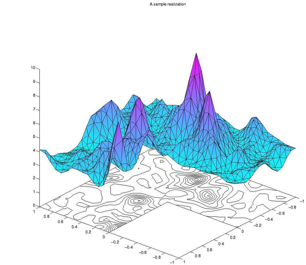
10 Realisation of κ(x, ω)

11 Stochastic PDE and Variational Form Insert stochastic parameters into PDE stochastic PDE (κ(x, ω) u(x, ω)) = f(x, ω), x G & b.c. on G Solution u(x, ω) is a stochastic field in tensor product form W S u(x, ω) = µ v µ (x) u (µ) (ω) = µ v µ (x)u (µ) (ω) W is a normal spatial Sobolev space, and S a space of random variables, e.g. S = L 2 (Ω, P ). Then W S L 2 (Ω, P ; W). Variational formulation: Find u W S, such that v W S : a(v, u) := v(x, ω) (κ(x, ω) u(x, ω)) dx dp (ω) = Ω Ω G [ G v(x, ω)f(x, ω) dx + G ] v(x, ω)g(x, ω) ds(x) dp (ω) =: f, v.

12 Mathematical Results 2 To find a solution u W S such that for v : a(v, u) = f, v is guaranteed by Lax-Milgram lemma, problem is well-posed in the sense of Hadamard (existence, uniqueness, continuous dependence on data f, g in L 2 and on κ in L -norm). may be approximated by Galerkin methods, convergence established with Céa s lemma Galerkin methods are stable, if no variational crimes are committed Good approximating subspaces of W S have to be found, as well as efficient numerical procedures worked out. Different ways to discretise: Simultaneously in W S, or first in W (spatial), or first in S (stochastic).

13 Computational Approach 3 Principal Approach:. Discretise spatial (and temporal) part (e.g. via finite elements, finite differences). 2. Represent computationally stochastic fields which are input to problem. 3. Compute solution/statistics: Directly via high-dimensional integration (e.g. Monte Carlo, Smolyak, FORM). Or approximate solution with response-surface, then integration Variational formulation discretised in space, e.g. via finite element ansatz u(x, ω) = n l= u l(ω)n l (x) = [N (x),..., N n (x)][u (ω),..., u n (ω)] T = N(x) T u(ω): K(ω)[u(ω)] = f(ω). Remark on Computing with Averages: Ku = f K u, as K and u are not independent, but if K and f are independent u = K f = K f K u = f

14 Example Solution 4 Geometry 2.5 flow = flow out.5 2 Sources Dirichlet b.c Realization of κ Realization of solution Mean of solution Variance of solution x Pr{u(x) > 8}.5 y.5

15 First Summary 5 Probabilistic formulation to quantify uncertainty, or find variation / distribution of response, Mathematical formulation in variational form gives well-posed problem Numerical approach may first perform familiar space / time semi-discretisation, Computational representation of input stochastic fields is needed, Statistics / Expectations may be computed either through direct integration with various methods (best known is Monte Carlo) or indirectly by first computing representation of solution u(ω) in terms of stochastic input, and then perform integration

16 Computational Requirements 6 How to represent a stochastic process for computation, both simulation or otherwise? Best would be as some combination of countably many independent random variables (RVs). How to compute the required integrals or expectations numerically? Best would be to have probability measure as a product measure P = P... P l, then integrals can be computed as iterated one-dimensional integrals via Fubini s theorem, Ψ dp (ω) = Ω... Ω Ψ dp (ω )... dp l (ω l ) Ω l

17 Random Fields 7 Consider region in space G, a random field is a RV κ x at each x G, alternatively for each ω Ω a random function a realisation κ ω (x) on G Mean κ(x) = E (κ ω (x)) now a function of x and fluctuating part κ(x, ω). Covariance may be considered at different positions C κ (x, x 2 ) := E ( κ(x, ) κ(x 2, )) If κ(x) κ, and C κ (x, x 2 ) = c κ (x x 2 ), process is (weakly) homogeneous. Here representation through spectrum as a Fourier sum or integral is well known. We have to deal with another function (RV) at each point x! Need to discretise spatial aspect (generalise Fourier representation). One possibility is the Karhunen-Loève Expansion. Need to discretise each of the random variables in Fourier synthesis. One possibility is the Polynomial Chaos Expansion.

18 Karhunen-Loève Expansion I 8 KL mode KL mode Eigenvalue-Problem for Karhunen-Loève Expansion KLE. Other names: Proper Orth. Decomp.(POD), Sing. Value Decomp.(SVD), Prncpl. Comp. Anal.(PCA): C κ (x, y)g j (y) dy = κ 2 jg j (x) G gives spectrum {κ 2 j} and orthogonal KLE eigenfunctions g j (x) Representation of κ: κ(x, ω) = κ(x) + κ j g j (x)ξ j (ω) =: κ j g j (x)ξ j (ω) = κ j g j (x) ξ j (ω) j= with centred, uncorrelated random variables ξ j (ω) with unit variance. Truncate after m largest eigenvalues optimal in variance expansion in m RVs. A sparse representation in tensor products. j= j=

19 Karhunen-Loève Expansion II 9 Singular Value Decomposition: To every random field with vanishing mean w(x, ω) W L 2 (Ω) (W Hilbert) associate a linear map W : W L 2 (Ω). W : W v W(v)(ω) = v( ), w(, ω) W = v(x)w(x, ω) dx L 2 (Ω). KLE is SVD of the map W, the covariance operator is C w := W W, and u, v W : u, C w v W = W(u), W(v) L2 (Ω) = ( E (W(u)W(v)) = E G G G u(x)w(x, ω) dx u(x)e (w(x, ω)w(y, ω)) v(y) dy dx = G G ) v(y)w(y, ω) dy G u(x) G = C w (x, y)v(y) dy dx The covariance operator C w is represented by the covariance kernel C w (x, y). Truncating the KLE is therefore the same as what is done when truncating a SVD, finding a sparse representation.

20 Representation in Gaussian Random Variables 2 How to handle the RVs {ξ j (ω)} in the KLE? In L 2 (Ω, P ) take the Hilbert subspace Θ of centred Gaussian RVs. Let {θ k (ω)} be an orthonormal (uncorrelated and unit variance) basis in the Gaussian Hilbert space Θ. For Gaussian RVs: uncorrelated independent. On a m-dimensional subspace Θ (m) = span{θ,..., θ m } we have (with the notation θ m (ω) = (θ (ω),..., θ m (ω)) R m ): Θ (m) can be represented by R m with a Gaussian product measure Γ m : dγ m (θ m ) = (2π) m/2 exp( θ m 2 /2) dθ m m m = dγ (θ j ) = (2π) /2 exp( θj 2 /2) dθ j j= j= Represent {ξ j (ω)} as functions of those Gaussian RVs, i.e. as functions of basis.

21 Polynomial Chaos Expansion 2 As Θ L p (Ω) p <, finite products of Gaussians are in L 2 (Ω): Theorem[Polynomial Chaos Expansion]: Any RV r(ω) L 2 (Ω, P ) can be represented in orthogonal polynomials of Gaussian RVs {θ m (ω)} m= =: θ(ω): r(ω) = ϱ (α) H α (θ(ω)), with H α (θ(ω)) = h αj (θ j (ω)), α J j= where J := N (N) = {α α = (α,..., α j,...), α j N, α := j= α j < }, are multi-indices, where only finitely many of the α j are non-zero, and h l (ϑ) are the usual Hermite polynomials. The series converges in L 2 (Ω). In other words, the H α are an orthogonal basis in L 2 (Ω), with H α, H β L2 (Ω) = E (H α H β ) = α! δ αβ, where α! := j= (α j!). H n = span{h α : α = n} is homogeneous chaos of degree n, and L 2 (Ω) = n= H n. Especially each ξ j (ω) = α ξ(α) j H α (θ(ω)) from KLE may be expanded in PCE.

22 Second Summary 22 Representation in a countable number of uncorrelated independent Gaussian RVs Allows direct simulation independent Gaussian RVs in computer by random generators (quasi-random), or direct hardware (e.g. sample noise from sound device). Each finite dimensional joint Gaussian measure Γ m (θ m ) is a product measure, allows Fubini s theorem (Γ m (θ) = m l= Γ (θ l )). Polynomial expansion theorem allows approximation of any random variable which depends on this representation, especially also the output / response u(x, ω) = u(x, θ), resp. in the spatially discretised case u(ω) = u(θ). Still open: How to actually compute u(θ)? How to perform integration? In which order?

23 Computational Approaches 23 The principal computational approaches are: Direct Integration (Monte Carlo) Directly compute statistic by quadrature: Ψ u = E (Ψ(u(ω), ω)) = Ψ(u(θ), θ) dγ (θ) by numerical integration. Θ Perturbation Assume that stochastics is a small perturbation around mean value, do Taylor expansion and truncate usually after linear or quadratic term. Response Surface Try to find a functional fit u(θ) v(θ), then compute with v. Integrand is now cheap. Stochastic Galerkin Use an ansatz for the solution u(θ) = β u(β) H β (θ) in the stochastic dimension, then do Galerkin method to obtain u (β). Observe that this is one possible functional form of response surface.

24 Stability Issues 24 For direct integration approaches direct expansion (both KLE and PCE) pose stability problems: Both expansions only converge in L 2, not in L (uniformly) as required spatially discrete problems to compute u(θ z ) for a specific realisation θ z may not be well posed. Convergence of KLE may be uniform if covariance C κ (x, x 2 ) smooth enough. E.g. not possible for C κ (x, x 2 ) = exp(a x x 2 + b) here for truncated KLE there are always regions in space where κ is negative. Truncation of PCE gives a polynomial, as soon as one α j is odd, there are θ j values where κ is negative compare approximating exp(ξ) with a truncated Taylor poplynomial at odd power. This can not be repaired. Like negative Jacobian in normal FEM. For methods which directly require u(θ z ) for a specific realisation, transformation method κ(x, ω) = φ(x, γ(x, ω)) possible with KLE of Gaussian γ(x, ω).

25 Stochastic Galerkin I 25 Recipe: Stochastic ansatz and projection in stochastic dimensions u(θ) = β u (β) H β (θ) = [..., u (β),...][..., H β (θ),...] T = uh(θ) Goal: Compute coefficients u (β). Directly through projection as explained, has problems. 2. Through stochastic Galerkin Methods (weighted residuals), α : E ( H α (θ)(f(θ) K(θ)u(θ)) ) =, requires solution of one huge system, only integrals of residua 3. For stochastic Galerkin methods the convergence issues of KLE and PCE may be solved. A (forgivable) variational crime like numerical integration in normal FEM.

26 Stochastic Galerkin II 26 Of course we can not use all α J, but we limit ourselves to a finite subset J k,m = {α J α k, ı > m α ı = } J. Let S k,m = span{h α : α J k,m }, ( ) m + p + then dim S k,m = p + m k dim S k,m

27 Third Summary 27 Integration may require many evaluations of integrand, if combined with expensive to evaluate integrand tremendous effort (this hits direct Monte Carlo). Direct integration and response surface method is conceptually simple, but may have stability problems. Stochastic Galerkin methods require solution of huge system, and a bit more changes to existing programs. Stochastic Galerkin methods require only much cheaper integrands of residua. Stochastic Galerkin methods are stable (here (variational) crime pays).

28 Results of Galerkin Method 28 err. 4 in mean m = 6 k = x.5 y.5 err. 4 in std dev m = 6 k = x.5 y.5 u (α) for α = (,,,,, ) x y Error 4 in u (α) Galerkin scheme x y

29 Galerkin-Methods for the Linear Case 29 α satisfy: [ β G N(x) E (H α (θ)κ(x, θ)h β (θ)) N(x) T dx ] u (β) = E (f(θ)h α (θ)) }{{} =:α! f (α) More efficient representation through direct expansion of κ in KLE and PCE and analytic computation of expectations. κ(x, θ) = κ j ξ j (θ)g j (x) j= r κ j ξ j (γ) H γ (θ)g j (x). γ J 2k,m j=

30 Resulting Equations 3 Insertion of expansion of κ ( α satisfy): κ j ξ j (γ) E (H α H β H γ ) N(x) g }{{} j (x) N(x) T dx β γ j }{{} =: (γ) α,β K j u (β) = α! f (α) K j is a sparse stiffness matrix of a FEM discretisation for the material g j (x). As j, κ j, and as γ, ξ (γ) j. The Hermite polynomials form an algebra, i.e. H β H γ = ɛ c(ɛ) β,γ H ɛ; the c (ɛ) known, they are the structure constants of the Hermite algebra. Therefore the matrix (γ) = ( (γ) α,β ) may be evaluated analytically. (γ) α,β = E ( H α ɛ c (ɛ) β,γ H ɛ ) = ɛ c (ɛ) β,γ E (H αh ɛ ) = ɛ β,γ are c (ɛ) β,γ α! δ αɛ = α! c (α) β,γ

31 Tensor Product Structure 3 The equations have the structure of a Kronecker or tensor product κ j ξ j (γ) (γ) α,β K j (γ) α 2,β K j (γ) α,β 2 K j (γ) α 2,β 2 K j u(β ). = γ j..... u (β N) f (α ).. f (α N) or with tensors u = [u (β),..., u (βn) ] and f = [f (α),..., f (αn) ] K u = κ j ξ j (γ) (γ) K j u = f j γ #dof space #dof stoch linear equations (curse of dimensions). Exploit parallelism in the multiplication, parallel operator-sum Block-matrix efficiently stored and used in tensor-representation.

32 Sparsity Structure of 32 Non-zero blocks for increasing degree of H γ

33 Approximation Theory 33 Stability of discrete approximation under truncated KLE and PCE. Matrix stays uniformly positive definite. Convergence follows from Céa s Lemma. Convergence rates under stochastic regularity in stochastic Hilbert spaces stochastic regularitry theory?. Error estimation via dual weighted residuals possible. Stochastic Hilbert spaces start with formal PCE: R(θ) = α J R(α) H α (θ). Define for ρ and p norm (with (2N) β := j N (2j)β j ): R 2 ρ,p = α R (α) 2 (α!) +ρ (2N) pα.

34 Stochastic Hilbert Spaces Convergence Rates 34 Define for ρ, p : (S) ρ,p = {R(θ) = α J R (α) H α (θ) : R ρ,p < }. These are Hilbert spaces, the duals are denoted by (S) ρ, p, and L 2 (Ω) = (S),. Let P k,m be orthogonal projection from (S) ρ,p into the finite dimensional subspace S k,m. Theorem: Let p >, r > and let ρ. Then for any R (S) ρ,p : R P k,m (R) 2 ρ, p R 2 ρ, p+r c(m, k, r) 2, where c(m, k, r) 2 = c (r)m r + c 2 (r)2 kr. dim S k,m grows too quickly with k and m. Needed are sparser spaces and error estimates for them.

35 Matrix Expansion Errors 35 H γ is orthogonal on polynomials of degree < γ (γ) αβ = E (H αh β H γ ) = hence sum over γ is finite. for γ > α + β, K j in a finite dimensional space One can choose J such that expansion J κ j ξ j (γ) (γ) K j u j= γ is arbitrarily close to = N(x) E (κ(x, θ)h α (θ)h β (θ)) N(x) T dx u (β), β G and hence global matrix uniformly positive definite. This stability argument is only valid for the Galerkin method.

36 Properties of Global Equations 36 K u = j α κ j ξ j (α) (α) K j u = f Each K j is symmetric, and each (α). Block-matrix K is symmetric. SPDE ist positive definite. Appropriate expansion of κ K is uniformly positive definite stability. Solving the Equations: Never assemble block-matrix explicitly. Use K only as multiplication. Use Krylov Method (here CG) with pre-conditioner.

37 Block-Diagonaler Pre-Conditioner 37 Let K = K = stiffness-matrix for average material κ(x). Use deterministic solver as pre-conditioner: P = K = I K... K Good pre-conditioner, when variance of κ not too large. Otherwise use P = block-diag(k). This may again be done with existing deterministic solver. Block-diagonal P is well suited for parallelisation.

38 Parallelising the Matrix-Vector Product 38 α : (K u) (α) = J j γ β κ j ξ (γ) j (γ) α,β K j u β K j = deterministic solver. This may be a (lower-level) parallel program to do K j u β. Parallelise operator-sum in j several instances of deterministic solver in parallel. Distribute u and f Parallelise sum in β. Sum in α may also be done in parallel, but usually not essential.

39 Further Sparsification 39 One term of matrix vector product may also be written as κ j ξ (γ) j (γ) K j u = κ j ξ (γ) j K j u( (γ) ) T. Use discretised version of KLE of right hand side f(ω) with KLE eigenvectors f l : f(ω) = f + ϕ l φ l (ω)f l = f + ϕ l φ (α) l H α (ω)f l. l l α In particular α! f (α) = l ϕ l φ (α) l f l. As ϕ l, only a few l are needed. Let φ = (φ (α) l ), ϕ = diag(ϕ l ), and ˆf = [..., f l,...]; then the SVD of f(ω) is f = [..., f (α),...] = ˆfϕφ T = l Similar sparsification needed for u via SVD with small m: ϕ l f l φ l. u = [..., u (β),...] = [..., u m,...]diag(υ m )(y (β) m ) T = ûυy T. Then K j u( (γ) ) T = (K j û)υ ( (γ) y) T is much cheaper.

40 Computation of Moments 4 Let M (k) f k { times }}{ = E f(ω)... f(ω) = E ( f k ), or clearer (as M (k) f is symmetric) M (k) f = E ( f k ), with M () f = f and M (2) f = C f and symmetric tensor product. KLE of C f is C f = l ϕ l f l f l. For deterministic operator K, just compute Kv l = f l, and then Kū = f, and ( M (2) u = C u = E ũ k) = ϕ l v l v l. l As ũ(ω) = l α ϕ l φ (α) l M (k) u = k l... l k m= H α (ω)v l, it results that k ϕ lm α (),...,α (k) n= ) φ α (n) l n E (H α() H α(k) v l... v lk.

41 Non-Linear Equations 4 Example: Use κ(x, u, ω) = a(x, ω) + b(x, ω)u 2, and a, b random (similarily as before). Space discretisation generates a non-linear equation A( β u(β) H β (θ)) = f(θ). Projection onto PCE: a[u] = [..., E H α (θ)a( β u (β) H β (θ)),...] = f = ˆfϕφ T Expressions in a need high-dimensional integration (in each iteration), e.g. Monte Carlo or Smolyak (sparse grid) quadrature. After that, a should be sparsified or compressed. The residual equation to be solved is r(u) := f a[u] =.

42 Solution of Non-Linear Equations 42 As model problem is gradient of some functional, use a quasi-newton (here BFGS with line-search) method, to solve in k-th iteration ( u) k = H k r(u) u k = u k + ( u) k H k = H + k (a j p j p j + b j q j q j ) j= Tensors p and q computed from residuum and last increment. Notice tensor products of (hopefully sparse) tensors. Needs pre-conditioner H for good convergence: May use linear solver as described before, or just preconditioner (uses again deterministic solver), i.e. H = Dr(u ) or H = I K.

43 Fourth Summary 43 Stochastic Galerkin methods work. They are computationally possible on todays hardware. They are numerically stable, and have variational convergence theory behind them. They can use existing software efficiently. Software framework is being built for easy integration of existing software.

44 Important Features of Stochastic Galerkin 44 For efficency try and use sparse representation throughout: ansatz in tensor products, as well as storage of solution and residuum and matrix in tensor products, sparse grids for integration. In contrast to MCS, they are stable and have only cheap integrands. Can be coupled to existing software, only marginally more complicated than with MCS.

45 Outlook 45 Stochastic problems at very beginning (like FEM in the 96 s), when to choose which stochastic discretisation? Nonlinear (and instationary) problems possible (but much more work). Development of framework for stochastic coupling and parallelisation. Computational algorithms have to be further developed. Hierarchical parallelisation well possible.