INFLUENCE OF SPATIAL VARIATIONS OF RAILROAD TRACK STIFFNESS AND MATERIAL INCLUSIONS ON FATIGUE LIFE

Transcription

1 University of Nebraska - Lincoln DigitalCommons@University of Nebraska - Lincoln Mechanical (and Materials) Engineering -- Dissertations, Theses, and Student Research Mechanical & Materials Engineering, Department of 2015 INFLUENCE OF SPATIAL VARIATIONS OF RAILROAD TRACK STIFFNESS AND MATERIAL INCLUSIONS ON FATIGUE LIFE Celestin Nkundineza University of Nebraska - Lincoln, celestink@gmail.com Follow this and additional works at: Part of the Applied Mechanics Commons, Engineering Science and Materials Commons, Metallurgy Commons, Operations Research, Systems Engineering and Industrial Engineering Commons, Other Mechanical Engineering Commons, Structural Engineering Commons, and the Transportation Engineering Commons Nkundineza, Celestin, "INFLUENCE OF SPATIAL VARIATIONS OF RAILROAD TRACK STIFFNESS AND MATERIAL INCLUSIONS ON FATIGUE LIFE" (2015). Mechanical (and Materials) Engineering -- Dissertations, Theses, and Student Research This Article is brought to you for free and open access by the Mechanical & Materials Engineering, Department of at DigitalCommons@University of Nebraska - Lincoln. It has been accepted for inclusion in Mechanical (and Materials) Engineering -- Dissertations, Theses, and Student Research by an authorized administrator of DigitalCommons@University of Nebraska - Lincoln.

2 INFLUENCE OF SPATIAL VARIATIONS OF RAILROAD TRACK STIFFNESS AND MATERIAL INCLUSIONS ON FATIGUE LIFE By Celestin Nkundineza A Dissertation Presented to the Faculty of the Graduate College at the University of Nebraska In Partial Fulfillment of Requirements For the Degree of Doctor of Philosophy University of Nebraska Major: Mechanical Engineering and Applied Mechanics Under the Supervision of Professor Joseph A. Turner Lincoln, Nebraska November, 2015

3 INFLUENCE OF SPATIAL VARIATIONS OF RAILROAD TRACK STIFFNESS AND MATERIAL INCLUSIONS ON FATIGUE LIFE Celestin Nkundineza, Ph.D. University of Nebraska, 2015 Advisor: Joseph A. Turner Railroad transportation is very important for economic growth and effective maintenance is one critical factor for its economic sustainability. The high repetitive forces from a moving railcar induce cyclic stresses that lead to rail bending and potential deterioration due to fatigue crack initiation and propagation. Previous research for prediction of fatigue life has been done under the assumptions of a uniform track bed and a homogeneous rail. However the spatial variation of the track stiffness is expected to increase the maximum stresses in the rail and, therefore, accelerate the fatigue process. The research described in this dissertation is focused on the variations of the track modulus as well as the inclusions within the rail and their role on fatigue life. The computational procedure is based on the automated preprocessing and post processing of several hundreds of finite element models of the rail across a set of crossties chosen from a random ensemble with representative statistical variations. The model parameters are estimated from field track deflection dynamic measurement data in comparison with deflection data from FE models. A multiaxial fatigue model is used for the estimation of fatigue cycles to crack initiation while the extended finite element method (XFEM) is used for the computation of the crack propagation directions and the stress intensity factor range as the indicator of the crack propagation rate. The results show that a nonuniform track bed can reduce fatigue life up to 100 times in comparison with the behavior expected for a uniform trackbed. The role of inclusion stiffness relative to the background rail steel and inclusion location are both important for fatigue life. Both effects also influence the direction of the initiated crack propagation. The results of this work are expected to be used for the effective maintenance and scheduling of rail inspection.

4 i ACKNOWLEDGEMENT I would like to express my appreciations to my Advisor Dr. Joseph Turner for his time and patience, great technical guidance, significant feedbacks, review comments and mentorship he provided me through all the way of this research and dissertation writing. I would also like to appreciate Dr. Shane Farritor in collaboration with Dr. Sheng Lu for sharing the field measurement data and other relevant information that I used in this research. I would like to thank my Committee Members, Dr. Shane Farritor, Dr. Cho W. Solomon To and Dr. Elizabeth Jones for their time, patience, helpful suggestions and comments on my dissertation. I gratefully acknowledge the sponsors of my PhD studies including The Department of Mechanical and Materials Engineering at The University of Nebraska- Lincoln (UNL) and the Government of Rwanda. I would like to thank the following participants who provided support through education and techniques. 1) All Professors who taught me courses ranging from core engineering to entrepreneurship through which I gained education that sharpened my skills and proactivity perspectives necessary for this research work. 2) My research group members in QUISP lab for their helpful comments and suggestions. Thanks to all Turner Engineering Lab group members for all the helps I received. 3) My fellow graduate students that I interacted with for their thoughts. I would also like to thank my family members and friends for their support and shared joy. Last but not least thanks to Huskers for the Touch Downs!

5 ii LIST OF FIGURES Figure 1-1. Schematic showing the different planes to identify defect planes in relation to the rail section Figure 1-2. A picture that shows a transverse Fissure in the rail head [24] Figure 1-3. A picture that shows a compound fissure in the rail [24] Figure 1-4. Detail fracture originating from a shell [24] Figure 1-5. Half Moon Shaped Base [24] Figure 1-6. A schematic diagram of ultrasonic testing unit in Quantitative Ultrasonic for Inspection and Structural Prognosis (QUISP) Lab at UNL Figure 1-7. Fish plate joint Figure 2-1. Through-thickness crack in an infinite plate subject to a remote tensile stress Figure 2-2. Modes of fracture. (a) Mode I fracture, (b) Mode II fracture, (c) Mode III fracture [50] Figure 2-3. Stress components in the plane normal to the crack boarder (regenerated from [55]) Figure 2-4. Crack and crack tip contour represented in 2 dimensional coordinate system x1 x Figure 2-5. Definition of local orthogonal Cartesian coordinates at point s on the crack front, the crack is in x1 x3 plane [71]. x2 is perpendicular to the plane of crack. x1 is normal to the crack front, x3 is tangential to the crack front Figure 2-6. A schematic diagram of a typical fatigue crack growth stages (regenerated from [83]) Figure 2-7.Coordinates of normal direction to the principle plane of maximum principle stress, σ1along the vector n Figure 2-8. The variation of the constants Cσ, k and Cb with respect to values BA = R2/R1 [110] Figure 2-9. Fatigue and critical plane and related terminology in a specimen subjected to multiaxial loading Figure S-N curve for sequential law (regenerated from [94]) Figure 0-1. High speed train truck [147] Figure 0-2. A schematic to illustrate the elements of railway track Figure 0-3. Parts of the rail Figure 0-4. Load components on the rail Figure 0-5. Simulated wheel/rail impact force history at a rail joint [152] Figure 0-6. Winkler model for the rail on elastic foundation (regenerated from [153]).. 69 Figure 0-7. Pasternak foundation model for railroad track [182] Figure 0-8. (a) Example of un-discretized model. (b) Discretized model Figure 0-9. Transformation of element global coordinates (a) to element parametric coordinate system (b) Figure 0-10.Linear tetrahedral element Figure Quadratic tetrahedral element (10 nodes)

6 Figure Linear hexahedral element (8 nodes) Figure Quadratic hexahedral element (20 nodes) Figure Quadratic hexahedral element (27 nodes) Figure Rail-wheel contact modelling Figure Contact modelling of a rectangular block loaded by a loaded spherical block Figure Pressure distribution on the rail\wheel elliptic contact area due to the loaded wheel. The y axis is along lateral direction of the rail while the x axis is along longitudinal direction of the rail. The pressure distribution is therefore σzz(x, y) if z is taken as vertical axis of the rail Figure Track section model used in finite element analysis of the rail stresses and deformations Figure Maximum of principal stresses (max(σ1)) in the rail discretized at different global element sizes Figure Some of the stress tensor elements in rail FE model at different global element sizes Figure Normal stress profiles (MPa): (a) σ1 on top view of the rail (b) σxx contour plot on top view of the rail (c) σyy contour plot on top view of the rail (d) σzz contour plot on top view of the rail (e) σzz contour plot on side view of the rail cross section through which passes the vertical plane Figure Shear stresses: (a) von Mises Stress, (b) σxy and (c) σyz on a zoomed in rail cross-section under the load application surface area Figure XFEM of the rail track section model with crack at the base of the rail Figure (a) A right side view, (b) a left side view and (c) view from rail bottom of normal longitudinal stress distribution around the rail base crack. Left side is the side of load application Figure J integral from contours 4 to 8 for a crack length a = 1 mm. The first contour has a radius of 1 mm as the element size. Contours are then equally spaced by the same distance which is equal to the first contour radius Figure J integral from contours 4 to 8 for a crack length a =5.0 mm Figure J- Integral at different contours taken at crack edge point located at x = mm, where x is the lateral axis with originating from the rail vertical centerline Figure J- Integral of different contours taken at crack edge middle point (x = 0.0) Figure Averaged stress intensity factors over the last 5 contours for a crack length a = 4.0 mm Figure Averaged stress intensity factors over the last 5 contours for a crack length a = 6.0 mm Figure The maximum averaged stress intensity factor with respect to the crack length Figure Directions of crack propagation along the crack front for crack sizes a = 2.5 mm, a = 4.0 mm and a = 6.0 mm iii

7 Figure 4-1. (a) and (b) Schematic diagram of UNL equipment working principle for vertical track deflection measurement (regenerated from [43]). (c) Instrumentation and location of rail deflection measurement equipment [44] Figure 4-2. Relative deflection measurement data of the rails (Courtesy of MRail,Inc [243]) Figure 4-3 (a) The dimensions of the rail half cross section in mm, (b) The dimensions of the crosstie section in mm Figure 4-4. Rail contact patch area for wheel load application and its local coordinate system Figure 4-5. Boundary conditions: Displacement constraints and load applications on the model Figure 4-6. Displacement constraint conditions, a case with unconstrained displacements at the rail end sides. L=533.4 mm Figure 4-7. Displacement constraint conditions, a case with periodic displacement constraint conditions at the rail end sides Figure 4-8. Rail vertical deflection profile with free ends boundary conditions Figure 4-9. Rail vertical deflection profile with periodic boundary conditions at the ends Figure Deflection versus crosstie moduli relationship Figure Maximum principal stress fringes on the model Figure Relationship of maximum principal stresses with respect to crosstie moduli variation for a uniform track bed Figure Relationship of von Mises stress with respect to crosstie moduli Figure Some of the stress tensor components with respect to crosstie modulus Figure Deflection relationship with respect to maximum stresses in the rail under varying uniform track support modulus ranging from 200 MPa to 300MPa Figure Relationship of rail maximum principal stress with respect to the ratio of crosstie moduli Figure Relationship of maximum principal stresses with respect to the ratio of the crosstie moduli variation Figure Component of the stress tensor as the stiffness ratio in the crossties varies Figure The rail geometric simplification for the long rail model with rectangular cross-section and rectangular surface of load application Figure Gaussian distribution curves for some examples of randomly distributed crosstie moduli with a mean of: (a) 200 MPa and (b) 250 MPa. Oval points indicate numbers picked from data pool with a SD of 100 MPa and diamond points indicate numbers from a data pool with a SD of 40 MPa Figure 4-21 Examples of Gaussian distribution of crosstie moduli Figure A model that has average track moduli of 100 MPa, at a SD of 60 MPa and the load at position Figure A model that has average track moduli of 100 MPa, at a SD of 60 MPa and the load at position iv

8 Figure A model that has average track moduli of 100 MPa, at a SD of 60 MPa and the load at position Figure Relationship of the rail deflections with respect to the rail deflections average crosstie moduli Figure Relationship of the maximum stresses with respect to average crosstie moduli Figure Maximum deflections at different load positions under random track support moduli with a mean of 250 MPa and standard deviation (SD) of 96 MPa, first trial of the realization Figure Maximum deflections at different load positions under random track support moduli with a mean of 250 MPa and standard deviation of 74 MPa, first trial Figure Maximum deflections at different load positions under random track support moduli with a mean of 250 MPa and standard deviation of 60 MPa, first trial Figure Maximum deflections at different load positions under random track support moduli with a mean of 250 MPa and standard deviation of 22 MPa, first trial Figure Maximum longitudinal bending stress at different load positions under random track support moduli with a mean of 250 MPa and standard deviation of 96 MPa, first trial Figure Maximum longitudinal bending stress at different load positions under random track support moduli with a mean of 250 MPa and standard deviation of 74 MPa, first trial Figure Maximum longitudinal bending stress at different load positions under random track support moduli with a mean of 250 MPa and standard deviation of 60 MPa, first trial Figure Maximum longitudinal bending stress at different load positions under random track support moduli with a mean of 250 MPa and standard deviation of 22 MPa, first trial Figure Highest of maximum longitudinal stresses at different standard deviations of track support moduli Figure Average of maximum longitudinal stresses at different standard deviations of track support moduli Figure Maximum principal stress at different load positions under random track support moduli with a mean of 250 MPa and standard deviation of 96 MPa, first trial. 156 Figure Maximum principal stress at different load positions under random track support moduli with a mean of 250 MPa and standard deviation of 60 MPa, first trial. 157 Figure Maximum principal stress at different load positions under random track support moduli with a mean of 250 MPa and standard deviation of 22 MPa Figure Average of maximum principal stresses at different standard deviations of track support moduli Figure Maximum of maximum principal stresses at different standard deviations of track support moduli Figure Maximum principal stresses at different Gaussian simulations (results from a single realization at each standard deviation and mean) v

9 Figure Average of maximum principal stresses at different Gaussian simulations (results from a single realization at each standard deviation and mean) Figure Normalized number of loading cycles to fatigue crack initialization, normalized on number of cycles of a uniform Figure (a) Number for loading cycles and (b) Normalized number of cycles (normalized by number of fatigue cycles of a uniform track) to fatigue crack initialization at a given fatigue coefficient exponent b = and at different fatigue strength coefficients Figure Number of loading cycles to fatigue crack initiation in rail steels of different fatigue coefficient exponents and at a given fatigue strength coefficient of 936 MPa Figure Normalized number of fatigue loading cycles by maximum number of fatigue cycles in all cases as function of track support moduli with different rail steel fatigue coefficient exponent with fatigue strength coefficient of 936 MPa Figure Normalized number of fatigue loading cycles by maximum number of fatigue cycles in all cases as function of track support moduli with different rail steel fatigue strength coefficient at fatigue coefficient exponent b= Figure Normalized number of minimum fatigue loading cycles (reduction factor of fatigue cycles from the maximum possible fatigue cycles) at different fatigue coefficient exponents Figure Normalized number of minimum fatigue loading cycles (reduction factor of fatigue cycles from the maximum possible fatigue cycles) at different fatigue strength coefficients and at fixed fatigue coefficient exponent b= Figure Contour plot of von Mises stresses on exaggerated deformed rail crack view from the top of the rail Figure Stress intensity factor along a semi elliptical crack defined by major axis z1 = 5 mm (on z axis) and y1 =3 mm (on y axis) Figure Effective stress intensity factors with respect to the longitudinal axis Figure Crack propagation directions. Red arrows: crosstie moduli ratio = Figure All mode of fracture SIFs with uniform track modulus Figure Effective stress intensity factors at the elliptic crack edge points. The x axis is the rail lateral taking origin from the rail vertical mid-plane. y axis is the rail vertical axis from that takes origin from the rail Figure Maximum effective stress intensity factor with respect to track modulus ratio of the crosstie moduli Figure 5-1. Example of transverse cross section of the track FE model with inclusion. xf = 14.8 mm. F is the wheel load. (x, y) is global coordinate of the track in transverse plane. (x, h) is position coordinate for the rail inclusion position with origin at the top point on the rail running surface Figure 5-2 (a) Stress profile in the rail cross section with inclusion, σ1(y, z). (b) zoomed in stress profile in the neighborhood of the inclusion, σ1(y, z). (c) Stress profile around inclusion side towards negative z axis σ1y, +z, (d) Stress profile around inclusion side towards positive z axis σ1(y, z) vi

10 Figure 5-3. Absolute maximum principal stress concentration factor with respect to ratio of inclusion material modulus E to the rail material modulus Es Figure 5-4. Maximum principal stress profile across inclusions (E = 386 GPa) at central vertical axis (x = 0). (a) h = 10 mm, (b) h = 30 mm Figure 5-5. Maximum principal stress profile across inclusions (E = 386 GPa) at central vertical axis (x = 0). (a) h = 50 mm, (b) h = 70 mm, (c) h = 90 mm, (d) h = 110 mm. 187 Figure 5-6. Examples of models of with introduced inclusions at h = 30 mm. (a) x = -28 mm, (b) x = -16 mm, (c) x = 16 mm, (d) x = 28 mm Figure 5-7. Example of models of with introduced inclusions (E = 386 GPa) at h = 30 mm. (a) x = - 28 mm, (b) x = - 16 mm, (c) x = 16 mm, (d) x = 28 mm Figure 5-8. Examples of FE models of with introduced inclusions (E = 386 GPa) in the web offside of the centerline. (a) x = - 4 mm and h = 60 mm (b) x = 4 mm and h = 60 mm,(c) x = - 4 mm and h = 100 mm ; (d) x = 4 mm and h = 100 mm Figure 5-9. (a) Stress concentration factors in the head of the rail with stiff inclusion stiffer inclusion (E = 386 GPa). The x distance represents the lateral position from the rail centerline. h represents the vertical position from the rail top surface. (b) Example of inclusion in a model and its position illustration Figure (a)the stress concentration factors due to a stiff inclusion (E/Es = 1.9) at different locations in middle of the head and web of the rail. The horizontal axis is the vertical distance from the top rail surface towards the rail foot. (b) Illustration of x and h variation along the rail cross section Figure 5-11.x, y, z components of unit vector normal to the maximum principal plane normal to the maximum principal stress around (a) stiff inclusion (E/Es = 1.9) and (b) soft inclusion (E/Es = 0.5) along the vertical centerline (x=0.0). α1 is the angle between the vector to the x axis, β1 is the angle between the vector and the y axis and γ1 is the angle between the vector and the z axis Figure x, y, z Components of unit vector normal to the maximum principal plane normal to the maximum principal stress around (a) stiff inclusion (E/Es = 1.9) and (b) soft inclusion (E/Es =0.5) along a vertical line at x = 4 mm. α1 is the angle between the vector to the x axis, β1 is the angle between the vector and the y axis and γ1 is the angle between the vector and the z axis Figure x, y, z components of unit vector normal to the maximum principal plane normal to the maximum principal stress around (a) stiff inclusion (E/Es =1.9) and (b) soft inclusion (E/Es =0.5) along a vertical line at x = - 4 mm. α1 is the angle between the vector to the x axis, β1 is the angle between the vector and the y axis and γ1 is the angle between the vector and the z axis. h is the distance from rail top surface to the inclusion center Figure 5-14.Vector orientations of maximum principal stresses in the rail boundaries surrounding (a) stiff inclusion, (b) soft inclusion vii

11 viii LIST OF TABLES Table 4-1. Average relative deflections of the track at different section (Courtesy of MRail,Inc) Table 4-2. Maximum principal stresses and their principal plane normal directions for crosstie moduli with a mean of 150 MPa and a SD of 60 MPa Table 5-1 Stress concentration factors in the mid region of the rail in a presence of soft inclusion (E/Es = 0.5). x is the lateral distance from the vertical mid centerline, h is the vertical distance from the rail top surface Table 5-2. Stress concentration factors in the mid region of the rail in a presence of soft inclusion (E/Es = 0.5) Table 5-3 Fatigue life factor due to the presence of stiff inclusion in the rail head Table 5-4. Fatigue life factor due to the presence of stiff inclusion in the mid region of the rail cross section

12 ix TABLE OF CONTENTS LIST OF FIGURES... II LIST OF TABLES... VIII CHAPTER 1: INTRODUCTION Impact of railroad to economic growth Rail problems Railroad track maintenance and scheduling Inspection operations in railroad transportation Outline of the Dissertation CHAPTER 2: FRACTURE MECHANICS AND FATIGUE LIFE PREDICTION Basics of fracture mechanics Analytical solution of stress intensity ranges around elliptic cracks Computation of stress intensity factors from J - Integrals Fracture criterion for a three dimensional elliptic crack Review of fatigue life prediction Effective stress intensity factor analysis Stress based fatigue life prediction Stresses in rail Multiaxial fatigue life Probabilistic approaches for fatigue life prediction Review of cracks initiated at inclusions and railroad fatigue crack life predictions CHAPTER 3: MODELLING OF COUPLED TRAIN TRACK MECHANICS Train/track components description Rail Loads Impact loads Principal of load transfer Review of analytical modelling of train track dynamics Distributed parameter modelling Finite Element Method for Track Mechanics Types of elements for 2D and 3D solid meshing... 81

13 x Finite element for railroad track structural analysis implemented in Abaqus Finite element for rail fatigue fracture mechanics Summary CHAPTER 4: INFLUENCE OF SPATIAL VARIATIONS OF TRACK STIFFNESS ON RAIL STRESS AND FATIGUE LIFE Introduction Spatial variation of track stiffness and influence to train track performance Measurement of track stiffness, modulus and deflection Static measurements Dynamic measurements of track stiffness and deflections Track modulus statistics and their impact on track fatigue life Uniform and nonuniform track support modulus Long track section with randomly distributed track support moduli Computed results for long track model Variation of mean track modulus Influence of varying standard deviation of track support modulus Impact of track stiffness statistics on fatigue Nonuniform short track section and fatigue crack initiation Impact of track modulus variation over a long track on fatigue crack initiation Impact of track modulus variation on crack propagation rate and directions Summary CHAPTER 5: INFLUENCE OF INCLUSIONS IN RAIL Introduction Stress concentration due to an inclusion Influence of inclusion locations on stress concetration The spatial distribution of stress concentration factors Orientation of maximum principal plane around inclusions Impact of inclusions on fatigue crack initiation and propagation Summary CHAPTER 6: CONCLUSIONS AND FUTURE PROJECTIONS

14 xi REFERENCES APPENDICES Appendix A. Computational details for long track model: A flow chart for the preprocessing Appendix B. Computational details for long track model: pre-processing script and programming Appendix C. Computational details for long track model: post-processing script Appendix D. Computational details for short track model with inclusions: Example of pre-processing scripts and programming.... Error! Bookmark not defined.

15 1 CHAPTER 1: INTRODUCTION 1.1 Impact of railroad to economic growth Railroad systems have been an important factor for technological progress [1] that raised the worldwide economy to another level relative to other means of transportation. Different approaches to evaluate how railroads impacted economies of the countries have been analyzed by different authors. Some of these approaches include social savings [2], growth accounting techniques [3] which is based on estimating the Total Factor Productivity (TFP) growth to measure the contribution of technological change to economic growth, and market access approach [4]. All these approaches have found that railroad transportation somehow has contributed to economic growth in all countries where they were implemented. The very first prominent analysis of railroad impact to the economies of countries was done by Fogel [2]. In this analysis it was demonstrated that railroad transportation contributed to economic growth by generating social savings. The social savings were calculated based on the estimated additional cost for transport of the railroad output from one year using the next best alternative. The social savings are thus estimated as (P ALT P FC ) Q FC 1-1 where P FC and P ALT are respectively the price of railroad and alternative means of transport, and Q FC is the railroad transport output in the reference year. In case of countries lacking alternative cheap transportation, such as waterways, inferring landlocked countries, the social saving would be high because the price of alternative transportation would be very high. In case of developing countries and poor countries, the demand of transportation is high which means Q FC is large and therefore increases the social savings. The next best alternative transportation option was evaluated to be waterways. The findings showed that the railroads increased the social savings in most of the countries of

16 2 the world where they were implemented. Not only did the railroad transportation contribute highly to economic growth of developing countries and countries which lacked the presence of waterways but also it contributed to the economic growth of the developed countries and that had enough waterways. For example, a country like the United States with enough waterways, the social saving was estimated to be 3.7 % while countries with fewer waterways like Mexico the contribution of railroads to economic growth through social savings was estimated to be 38.5% [3]. Beginning transportation used waterways in the Unites States [5], however waterways faced constraints because of their locations and seasonal availability. In the same study conducted by [5] the challenges of railroad fuel economy and fuel efficiency while meeting the requirements of pollution control are addressed. It was recognized that as compared to other modes of transportation, railroads require less energy and emit fewer pollutants. Nevertheless, historians and economists including [3], [6] have been reluctant to accept this criterion due to the fact that despite social savings, many railroads suffered financial problems, and some railroad networks were not exploited fully. Rather, a new approach described in [3] was used to evaluate the impact of railroads on economic growth in Spain. The findings were that despite the predicted high impact of railroad on Spanish economy, the growth accounting technique found that the impact of railroads on the Spanish economic growth was less not as significant. This technique is founded on measuring the impact of a technological change to economic growth based on estimation of the Total Factor Productivity (TFP) growth [5] as a function of technological change (in this case the railroad transportation) inputs and outputs. This TFP is also known as the Solow Residual (ΔA/A) and is derived from the expression Y = K s K L s L A, 1-2 where Y is the total output, K denotes the service provided by capital stock, L is the total number of hours worked, and s K and s L are the factor income shares of labor and capital, respectively.

17 3 By taking the logarithm of both sides of Eq. 1-2 and differentiating the result with respect to variables Y, K, L, one obtaines a differential equation which can be changed into a difference equation that is a typical Cobb-Douglas production function as ΔY Y = s K ΔK K + s L ΔL The analysis based on Eq. 1-3 led to the understanding that the railroads contributed less to economic growth in Spain due to the reason that railroad transport had less importance in Spanish GDP before L + ΔA A 1-3 Ronaldson and Hornbeck [3] did an analysis of the historical impact of railroads on the American economy. They analyzed the railroad network access county by county and compared their agricultural land values with railroads transportation and without them. Agricultural lands values dropped by 64%; and the expansion of waterways and roads reduced this loss by 13% to 20%. Therefore their overall conclusion was that railroads impacted the American economy by reinforcing market access resulting in a reduced expression for general equilibrium of economic trade theory. After the birth of railways, there were developments in the construction of industries and engines, in civil engineering, communications etc. Railroads acted as a major force to American economic development by being an idea, construction enterprise and a producer and construction enterprise [7]. The railroad idea led many entrepreneurs and enterprisers to entertain new innovative plans, with enhanced hopes and new ways of conceiving the future. As a construction enterprise, the construction of railroad stimulated supply and demand. It stimulated labor, goods production for labor, capital and land. Supplies included market goods to laborers, investments for construction capital, labor salaries and the unused lands. The railroad as a producer and transportation service, carried passenger and freight at lower cost and higher volume than other means of transportation. Petersen [8] described the freight transport under globalization and its impact to Africa. Globally transport was a key role for economic growth of countries until the 1970s when it dropped down due to emerging telecommunication technologies that replaced some of the transport activities. Nevertheless transport regained again and was seen to appear as

18 4 an important element in factors for economic growth in the 1990s due to the economic restructuring that was characterized by standardization of production and distribution systems which necessitated improved transport technologies. On the other hand improved transport technologies reduced transport costs; and contrarily a lack of proper management and maintenance of transport infrastructures will hinder the reduction of transport costs. Railroads can contribute to economic growth better than roads if rail infrastructures is well managed. Historically, railroads were introduced in Africa during colonialization. According to the study conducted by Jedwab and Morari [9], after independence in many African countries, railroads were characterized by poor maintenance; nevertheless, this study concluded that many cities in Africa which were served by railroad lines were characterized by greater economic growth than cities which were not reached by railroads. The supply and demand of the economy based on railroad transportation led to railway components that were subjected to repeated cyclic forces due to the axle loads and train speeds which kept increasing with time as the economy reached a higher level. Therefore rails started to break down. German engineer Wöhler [10] initiated the field of fatigue analysis after realizing that many railway axles were breaking due to fatigue. Later on with other incidents in different structures such as aircraft components, rocket motors, bridges, ships, and oil containers the endeavor of the research in fatigue design and the application of linear fracture mechanics took a higher level. Advances in fatigue and fracture mechanics along the railroads have been detailed by several authors. The field of fracture mechanics was developed and other fields involved with inspection such as those using ultrasonic and electromagnetic waves became of great interest. These developments resulted in new strategies for safety technology against failure of railroad components as well as in other fields thereby improving the service life of many products. 1.2 Rail problems Broken rails are major causes of derailments in North America. The derailments caused by rail damage result in loss of lives and tremendous damage costs with respect to the train, its freight and the track bed, resulting in a nontrivial impact on the economy. The

19 5 costs due to broken rails are discussed by Schafer and Barken [11]. An average of $525,000 per derailment incident is spent for track and equipment. Derailment cases include recent ones in Montgomery, West Virginia in February 2015, where 27 railcars carrying oil derailed and the leaking oil caught fire leading to evacuation of nearby residents. According to an FRA report, the derailment was caused by a vertical split head broken rail. Two previous inspections in December 2014 and another in January 2015 missed the identification of potential defects that would lead to the broken rail. Other cases include a Canadian National Train derailment in October 2013 due to rail fracture that initiated undetected despite rail flaw inspection that was conducted two months before [12]. The rail fracture in this incident was initiated due to the replacement of the low rail by a high rail to reduce the super-elevation in the curve. A high rail sits much higher in the track than a low rail. However the high rail experienced high stresses leading to the crack initiation and fast propagation. Another case is the Hartfield train derailment in the United Kingdom which was reported to have been caused by rail fracture. The investigation found out that the rail section where the fracture occurred had been fragmenting due to rolling contact fatigue (RCF). RCF is known to be a result of high stresses developed at the interface of the wheel and rail contact due to excessive forces exerted at this interface [13]. The excessive forces come primarily from the axle shifting relative to the rail too far to one side or the other particularly in curves and crossings. Another cause of RCF as described in [13] is the rail vehicle suspension especially the yaw stiffness which is the resistance to horizontal rotation of the train truck. The potential increase of RCF with increase in yaw stiffness can be explained by the fact that higher forces are required to deflect the suspension -which has higher lateral stiffness (yaw stiffness)- when the train is running on curves. Higher truck stiffness is necessary to provide stability of the rail vehicle when traveling at higher speed and therefore restricting the hunting motion. A softer suspension induces instability for a train traveling at higher speeds. Therefore the compensation for train stability comes at the expense of increased RCF that leads to fatigue crack initiation.

20 6 Research showed that 22.7 % of train derailments in United States during the period of were due to broken rails and welds [14]. As induced stresses get higher in the rail and above the critical stresses that the rail can support, the progression of existing defects in the rails will initiate, and also, cracks will initiate and propagate. Rail defects are inherent to different causes including the manufacturing processes, rail joint methods such as welding, cyclic loading, geometric conditions of the track and spatial track stiffness variations [15]. Rail fatigue cracks can initiate from flaws which are introduced in rail during manufacturing followed by cyclic stresses and can develop and propagate to a certain extent undetected until the rail fails completely. The growth and propagation of the fatigue cracks are driven by the number of developed stress cycles through loading. Not only are these stresses induced by passing the train loads but also by thermal expansion and compression. Manufacturing processes may introduce impurities of some chemical composition which turn into inclusions that may initiate cracks that can grow as the rail is loaded cyclically. After cracks initiate and grow to a certain size, they can be detected using ultrasonic tools and other inspection methods [16 19]. As described in [20] welding can introduce high carbon content liquid resulting in brittle cementite structure which can reduce the load carrying capacity of the weld. The rolling train introduces wear to the rail which in turn is enhanced by impact loads from the rolling stock. The geometric conditions that lead to rail failure include curves that carry high axle loads on high or low rail, hence leading to mechanical deformation or plastic flow of the rail head. Research has shown that track stiffness is another major factor for the rail degradation [21 23]. A stiffness that is too low can lead to high deflections of the rail hence causing increased bending stresses in the rail. A stiffness that is too high, also leads to increased wheel/rail contact stresses. There are many factors that influence rail defects and therefore it has been reported to be impossible to predict the rail service life accurately [24]. In order to describe different defects, specific terminology is used for different planes of defects and stress development in the rail [24]. The vertical plane is used to describe stresses developing in a vertical direction normal to the rail length. The horizontal

21 7 plane represents stresses developing horizontally along the rail. Defects which are in the horizontal planes are typically named horizontal defects. The transverse plane contains stresses developing transversally along the cross section of the rail. These planes are depicted in Figure 1-1. Figure 1-1. Schematic showing the different planes to identify defect planes in relation to the rail section. A defect type can be identified by its plane of development, origin and direction. There are many different defect types; a complete description can be found in [24]. The most critical defect types are defects that develop in the transverse plane including transverse fissure, compound fissure, and detail fracture. These defects develop in the transverse plane, usually are internal in origin and are not visibly identified until the defect progresses to the rail head. A transverse fissure such as the one depicted in Figure 1-2 spreads outwards as a smooth, bright, or dark round or oval surface in the transverse plane starting from a crystalline center or nucleus inside the head of the rail [24]. The compound fissure in Figure 1-3 starts internally from a horizontal separation of a longitudinal seam or inclusion inherent from manufacturing and develops longitudinally before it starts to

22 8 develop transversally upward or downward. This defect results in oblique failure and is considered to be the most hazardous rail defect. Figure 1-2. A picture that shows a transverse Fissure in the rail head [24]. Figure 1-3. A picture that shows a compound fissure in the rail [24]. A detail fissure which is represented in Figure 1-4 has its origin from shelly spots, head checks, or flaking near the surface of the rail head. It can also originate from a longitudinal seam or streak near the running surface on the gage side. It grows slowly to a size of 10 or 15 % of the rail head cross section before reaching rapid and complete failure. Web defects include a broken base that develops due to improper bearing of the tie plate. As discussed in [24] a broken base has two main types of failure: broken base and base failure. A broken base is normally a half-moon failure as shown in Figure 1-4. A base fracture results from a nick on the base, due to improper handling, leading to a visible identifiable progressive transverse fracture at the base of the rail. This progression can be slow until it reaches a greater distance in the rail section. On the other hand complete and sudden failure can occur after this fissure has progressed only a very small distance [24].

23 9 Figure 1-4. Detail fracture originating from a shell [24]. Figure 1-5. Half Moon Shaped Base [24]. Rail defect growth is classified as normal, rapid or sudden. In normal growth, the defect develops over a certain period of time in gradual stages and can be uninterrupted. Rapid growth means recent defect evolution in numerous small stages. Sudden growth means the defect has been developed recently in a few large steps. 1.3 Railroad track maintenance and scheduling Railroad track maintenance is a critical factor for rail transportation productivity and safety. Without proper maintenance there is a risk to passenger life or loss of goods such as oil or gas and train damage due deteriorated rails that are not maintained properly. Therefore railroad maintenance scheduling is designed to solve the problem of preventing any type of rail accidents while minimizing the costs. This problem has been discussed by [25 28]. Also, planning models for maintenance production have been reviewed in [29]. In the study conducted by Ferreira and Murray [25] in which a model of future maintenance activities in relation with current maintenance activities, and track deterioration was developed. They noted that in 1993/94, track maintenance productivity lagged behind standard maintenance practice by an estimated $62 million which represented 16% of potential operating cost savings if the best practice of maintenance was used. Therefore they noted that a need to have the best maintenance productivity to maximize the benefit of the railroad operator is indispensable. This need is coupled with

24 10 the need to understand the causes of track deterioration. With regard to this issue their study was focused on track degradation issues and related maintenance support tools. Therefore maintenance support tools are often developed optimally by considering the interrelations between different degradation model variables including track components and geometry, axle loads, speeds, tonnages, track standards, management practices, investment decisions and climate with track condition. In addition budgetary constraints and risk assessment are other constraints that include train delays, derailments, revenue impact and ride quality. It was shown that the track performance in a certain time period is a function of maintenance activity since the previous maintenance work, traffic activities and environmental factors [25]. 1.4 Inspection operations in railroad transportation Railroad health monitoring is very important for the railroad industry so that failures can be prevented as much as possible thereby improving the economics of railroad operations. There are different techniques to investigate rail health from its manufacturing to its use in service. Different researchers have been dedicated to the study of such approaches. For example Jeong [30] conducted a study of rail integrity emphasizing engineering analyses which were validated by laboratory and field testing. In this analysis an investigation of different defects developed in the rail were found to be the basis of rail integrity and were integrated in the scheduling of inspections. Current rail manufacturing methods use improved technology such as optical cameras, ultrasonic probes, and eddy current techniques to minimize the introduction of defects in the rails. The defects introduced by improper use and handling are considered to be random and therefore it is difficult to control them in a maintenance scheduling scheme. As discussed by many researchers in the past many of the rail failures are caused by rail fatigue damage. The causes of rail fatigue include cracks that develop and propagate to a certain extent unnoticed until the rail fails completely. The initiation of these cracks begins after a number of stress cycles have developed as the trains pass. These stresses are induced by application of the train loads through the contact of train wheels and the rail surface,

25 11 loadings due to thermal expansion and compression. Comprehensive studies of loading types on railroad rails have been described by several authors. The loading from the train wheels in contact with the rail initiate wheel rail surface stresses and rail deflection that initiate track defects and deterioration. The identification of flaws, defects and condition of the track is accomplished by railroad engineers using different established techniques. Ultrasonic and electromagnetic induction based tools are used to detect internal defects such as inclusion and cracks [19], [31], [32]. Ultrasonic techniques are also used to detect any longitudinal defect across the rail head such as vertical split in heads and shear defects. Ultrasonic testing has been identified as the mainstay of rail testing technique in United States since the 1950s after taking over the induction technique which was developed in the 1920s. The induction technique is still extensively used in some parts of the world such as Russia. The basic principle of ultrasonic techniques is that a beam of ultrasonic wave energy is sent into the rail and the reflected or scattered ultrasonic wave energy is analyzed using ultrasonic transducers [33], [34]. As illustrated in Figure 1-6 the ultrasonic wave is sent into a sample from an ultrasonic transducer. The transducer can be coupled with the specimen using direct contact coupling, air coupling or liquid coupling. When the wave hits the front wall not all of its energy is transmitted into the material but a part of it is reflected because of the change in transmission resistance of the medium quantified as impedance. The transmitted wave after reaching the back wall will be also reflected. The reflected waves are then received by the transducers. The reflected waves are quantified by considering their amplitudes and phase. Any reflected wave between the front and back walls would then indicate a flaw in the sample. However for heterogeneous materials as the wave propagates it keeps scattering. In some cases, the reflected scattered waves and reflected waves from defects are of the same amplitude and phase. Therefore it may be difficult to distinguish the flaws from the heterogeneity of the materials. Because the defects are not always predictable the ultrasonic wave energy can be sent at several incident angles so that the chance to detect a defect is maximized.

26 12 Ultrasonic unit accessories Display Backwall signal Ultrasonic sensor Frontwall signal Test sample Figure 1-6. A schematic diagram of ultrasonic testing unit in Quantitative Ultrasonic for Inspection and Structural Prognosis (QUISP) Lab at UNL. The electromagnetic wave induction technique[35] works on the principle that a current stream is sent into the rail via contact brushes, hence making the rail to be a part of the current flow circuit. If the current meets a defect, it will travel around it; the result will be a distortion of induced electromagnetic field associated with the current flow which is detected by a set of transducers and sensors. Visual defects detection techniques [16] are used to detect rail surface defects and other visible defects such as a broken or missing fastener, visible cracked crosstie, etc.

27 13 Visual defects detection includes techniques like eddy current method, computer vision [36] that uses tools such as optical cameras and lasers, and visual detection by human eyes. The advantage of visual defect detection systems is that they do not need contact coupling with the rail and therefore they are classified as non-contact inspection systems. The major disadvantage is that they are usually unable to detect internal defects. Eddy current detection systems can discover internal defects which are closer to the surface such as transverse cracks and spalls of the rail head [37]. Alternatively research work has been done to combine eddy current and ultrasonic techniques so that both internal defects and rolling contact fatigue defects can be detected simultaneously [38]. The basic principle of eddy current detection technique is that an open ferrite core is wound with the coils supplied with a high frequency current. If the ferrite core is placed at a distance less than 20 mm from an electric conducive material an eddy current will flow into that rail material in a plane perpendicular to the plane of the magnetic field produced by the alternating current flowing through the sensor coils. The density of the eddy current depends on the supply frequency and electromagnetic properties of the rail (conductivity and permeability), and the distance between the sensor and the rail surface. Any change in rail properties caused by flaws, for example, will change the density of the eddy current and therefore change the coupling magnetic flux. It is this change that will indicate the presence of defects. This change is discovered by measuring the impedance of the coil. As reported in [37], one problem of eddy current sensors is that they sometimes indicate false defects; for example, fishplate joints between two standard rails (refer to Figure 1-7) will not be distinguished from transverse cracks. One of the solutions to this problem is that a map of false defects including the mileage of their locations is carried together with eddy current sensor so that they can be eliminated from detected real defects.

28 14 Figure 1-7. Fish plate joint. Track deflection and track stiffness/modulus measurements are described in [39 46]. Track stiffness is defined as load per unit deflection of the rail. Track modulus is defined as the load per unit deflection of the substructure of the track. A track with low stiffness exhibits high deflection. High track deflections mean high bending moments which influence the fatigue of the track. Track stiffness is a combination of stiffness in the rail, stiffness of crossties, fasteners, rail pads, ballast, sub ballast, embankment fill and subsoil. The stiffness in one component is different from the stiffness in the other component. As a consequence the overall stiffness is nonlinear and changes with the amplitude and frequency of the load for a given longitudinal portion of the track. 1.5 Outline of the Dissertation This dissertation combines five chapters. The second chapter encompasses an extensive review of fracture mechanics theory and fatigue models. A particular emphasis is put on the derivations of stress intensity factors and stresses at the tip of elliptical cracks that develop in the rails more than other types of cracks. Also, in this chapter, fatigue models which are used for uniaxial loading and multiaxial loading are reviewed in two categories: fracture based fatigue models and fatigue based fatigue models. An introduction to the principal stress orientation is also given to provide a preliminary understanding of stress orientation angles that can be used for elliptical fatigue crack orientation in the rail in subsequent chapters. Also the rail wheel contact stresses which will be used in the finite element models are reviewed.

29 15 The third chapter consists of a description of the components of the coupled train track, interacting loads, finite element formulation and how it is applied in computational fracture mechanics. An example of the finite element analysis applied to rail track and the convergence study is given for the track models that will be used in the subsequent chapters. Also, the extended finite element formulation for cracks and an example of analyzing a stationary crack in the rails are given. The fourth chapter deals with the spatial variation of track stiffness and its influence on fatigue crack initiation and propagation. It starts with the review of track modulus estimation models and measurements techniques. After this, the model of the track support modulus using track deflection measurement data and short track finite element model with valid geometry of the rail. The effect of the variation of track support modulus in a short section of the track is also analyzed. After this, a long track model with randomly distributed track support modulus is studied by varying the statistics of the crosstie modulus in the range that allows rail deflections of same range as experimental measurements which results in automatic parameterized models. An analysis of the computationally generated vertical deflections, stresses, and effect to fatigue life is done with respect to these statistics. The fifth chapter entails the modeling and analysis of inclusions in the rail and their effect on fatigue life of the rail. Stiff inclusions as well as soft inclusions are introduced in the model one by one in each model at different positions in the rail cross section. The stresses around inclusions are investigated and their maximum values and orientations are extracted from the computational output. The orientation angles of higher stresses are used to predict the orientation of fatigue cracks emanating from rail inclusions which are thereafter introduced in the models are discussed. Finally, in chapter six, the results are summarized and conclusions are drawn.

30 16 CHAPTER 2: FRACTURE MECHANICS AND FATIGUE LIFE PREDICTION 2.1 Basics of fracture mechanics The basic idea of fracture mechanics theory originates from Griffith s work [47] that refers to the surface tension of liquids. He theorized that the surface of the solid also possesses surface tension energy which increases as the crack propagates thereby balancing the increase of externally or internally released energy. Griffith s balance theory states that d da (U V) = γ, 2-1 where U and V, respectively, are the work of external forces and elastic strain energy, A is the crack surface area and γ is the specific surface tension energy of the solid. Irwin [48] defined the measure of energy available for crack extension by an energy release rate G as G = d(u V). da 2-2 Therefore the energy release rate can be defined as the rate of released potential energy by fracture per unit area of crack surface. The potential energy in an elastic body is defined as Π = V U. 2-3 For example for a crack of length 2a in an infinite plate shown in Figure 2-1 subject to a remote tensile stress σ, the energy release rate G is given by [49] where E is the Young s modulus of the solid. G = πσ2 a E, 2-4

31 17 Figure 2-1. Through-thickness crack in an infinite plate subject to a remote tensile stress. For the fracture to occur the energy release rate must reach the critical energy release rate as a function of critical remote stresses and critical crack size. If the stress is fixed below the critical stress, then the crack size must reach the critical value in order for the critical energy release rate to be attained. Another alternative method is to express the available fracture energy in terms of asymptotic stress and displacement fields around the crack as [48], [49] σ ij ( K 2πr ) f ij(θ), 2-5 where σ ij is the Cauchy stress tensor, r is the distance from the crack tip, θ is the angle with respect to the plane of the crack, f ij are functions that depend on the crack geometry and loading conditions. K is called the stress intensity factor which basically depends on the crack and the solid geometry and the nature of the loading. The crack fractures in three modes: opening mode which is known as mode I fracture and is characterized by the stress intensity factor denoted as K I ; sliding mode known as mode II fracture and characterized by the stress intensity factor denoted as K II ; and, the tearing mode of fracture known as mode III fracture and characterized by the stress intensity factor K III. All these modes of fracture are depicted in Figure 2-2.

32 18 (a) (b) (c) Figure 2-2. Modes of fracture. (a) Mode I fracture, (b) Mode II fracture, (c) Mode III fracture [50]. For the plate in Figure 2-1, the stress intensity factor for mode I fracture is given by: K I = σ πa. 2-6 f ij as well as complete expressions of stresses near the crack tip were derived by Irwin [48] and a detailed review can be found in [49]. In the fracture mechanics field, the treatment of crack problems started by studying two dimensional crack propagation and the stress distribution around the crack tip. Irwin provided a well detailed derivation of stresses and stress intensity factors around a crack tip for this problem [48]. This study led to a knowledge that the stresses around the crack tip exhibit singularities proportional to the inverse square root of the distance from the crack edge to the point of stress considered. Later on fracture mechanics researchers started looking at cracks in three dimensional solids. The most popular crack configuration was a penny shaped crack. Investigators of this type of problem include Sneddon [51] who studied a crack oriented in a known orientation and obtained the stresses around the crack tip using the Hankel transform and Westermann [52] who looked at particular loading of shear stresses on the faces of cracks and obtained the stress and displacements fields.

33 Analytical solution of stress intensity ranges around elliptic cracks A more complicated configuration of three dimensional cracks is an elliptic shaped crack which is also encountered as an internal crack in rails. Green and Sneddon [53] were the first to study the stress distribution around an elliptical crack in solids subjected to symmetric normal loadings with respect to crack faces. They derived the analytical solution for stress distribution around the crack. Referring to this work Kassir and Sih [54] worked on a more general closed form solution of stress distribution around an elliptical crack in a three dimensional solid under arbitrally loading. The elliptic crack in a three dimensional solid subjected to the symmetric loading, with loads normal to the planes of the crack, are prone to propagation until reaching critical value of stress intensity factor K I of mode I fracture. The tearing and sliding modes of fracture are influenced by related stress intensity factors K II and K III for respective mode II and mode III fractures. Therefore to find the closed form solution of stresses and all SIFs of elliptical cracks under arbitrary loading Kassir and Sih [54] decomposed the problem into two parts: The case of the elliptic crack subjected to normal loading which allowed them to determine the expression of K I and the case of the same crack subjected to shearing loads which allowed them to provide the expressions of K II and K III. They postulated that the criterion of fracture does not depend solely on the critical value of K I but also on stress intensity factors K II and K III. Therefore the fracture criterion is assumed to be a value which is a function of the three SIFs. The approach of Kassir and Sih [54] focused on computing the stress distribution under arbitrary shear loads. The derivation started from choosing the harmonic functions that solve the equations of Navier displacements. Navier displacements equation is derived from the three main equations. These include the constitutive equation σ ij = λδ ij ε kk + 2με ij, 2-7 where λ and μ are the Lamé constants defined as

34 20 λ = Eμ (1 + ν)(1 2ν), μ = E 2(1 + ν). 2-8 the equation of elastic motion equilibrium σ ij x j + b i = ρa i, 2-9 and the strain displacement equation ℇ ij = 1 2 ( u i x j + u j x i ) The Navier displacement equilibrium equation is then obtained upon substituting the strain displacement equation into the constitutive equation and having the resulting relation substituted into the equilibrium equation of motion. The result is then: (λ + μ) 2 u j x j x i + μ 2 u i x j x j + b i = ρ 2 u i t Under equilibrium, and with neglecting the body forces, the Eq becomes (λ + μ). u + μ 2 u = 0, 2-12 where is the gradient operator, and u is the displacement vector. Eq is equivalent to writing with Eq when body forces are neglected (b i = 0) and if static equilibrium is considered ( 2 u i t 2 = 0).

35 21 z σ zz σ tz Crack σ nz σ nn σ nt θ σ tt r p n t Figure 2-3. Stress components in the plane normal to the crack boarder (regenerated from [55]). Kassir and Sih [54] assumed a displacement potential as u = φ + z ψ, 2-13 where φ and ψ are real harmonic functions, such that 2 φ = 0 and 2 ψ = The relations in Eq. 2-12, Eq and Eq led to expressing the displacements and stress components around an elliptical crack as functions of partial derivatives of the potential function as [54]. φ x = 2(1 ν) f z, φ y = 2(1 ν) g z, 2-15 φ z = (1 2ν)ψ,

36 22 ψ = f x + g y, The crack edge is defined by x 2 a 2 + y2 b 2 = 1, 2-16 and z = 0, where a and b are respectively the minor and major semi axes of an elliptic crack. A potential function of the form provided by Green and Sneddon [53] was used together with ellipsoidal coordinates. Whittaker and Whatson [56] demonstrated that the Cartesian coordinates (x, y, z) can be converted into ellipsoidal coordinates (ξ, ζ, η) using the following relations a 2 (a 2 b 2 )x 2 = (a 2 + ξ)(a 2 + ζ)(a 2 + η), b 2 (b 2 a 2 )y 2 = (b 2 + ξ)(b 2 + ζ)(b 2 + η), a 2 b 2 z 2 = ξζη where ξ, ζ and η are roots of an equation in s x 2 a 2 + s + y2 b 2 + s + z2 s 1 = 0, 2-20 and are bounded by: > ξ 0 ζ b 2 η a 2 The functions f and g were expressed in terms of a potential function H given as where f(x, y, z) = 1 AH(x, y, z), 2 g(x, y, z) = 1 BH(x, y, z),

37 23 H(x, y, z) = ( x2 a 2 + s + y2 b 2 + s + z2 s 1) ds ξ Q(s), 2-23 and Q(s) = s(a 2 + s)(b 2 + s), and, A and B are the coefficients to be determined. Therefore, referring to Figure 2-1 and performing lengthy manipulations through Eqs (or 2-11), 2-13, 2-15, 3-19, 2-21, 2-22 and 2-23, Kassir and Sih [54] obtained the stress field containing stress intensity factors as K I σ nn = (2r) 1 cos θ 2 (1 sin θ 2 sin 3θ 2 ) 2 (2r) 1 sin θ 2 (2 + cos θ 2 cos 3θ 2 ) 2 K II O (r 1 2), K I σ zz = (2r) 1 cos θ 2 (1 + sin θ 2 sin 3θ 2 ) + 2 (2r) 1 sin θ 2 cos θ 2 cos 3θ 2 + O (r1 2), 2 K I K II K II σ tt = (2r) 1 2ν cos θ 2 2 (2r) 1 2ν sin θ 2 + O (r1 2), σ nt = K III (2r) 1 2 sin θ 2 + O (r1 2), 2-27 K I σ nz = (2r) 1 2 sin θ 2 cos θ 3θ cos K II (2r) 1 cos θ 2 (1 sin θ 3θ sin 2 2 ) O (r 1 2), and K III σ tz = (2r) 1 cos θ 2 + O (r1 2) In Eqs , r is the radial distance from the point of intersection between the crack edge and its normal plane to the point considered in the plane normal to the crack edge and θ is the angle between that radial line and the crack plane. The stresses σ nn, σ tt and σ nt are related to Cartesian coordinates stresses σ xx, σ yy and σ xy through the relations [54]

38 24 σ nn = 1 2 (σ xx + σ yy ) (σ xx σ yy )cos 2β + σ xy sin 2β, σ tt = 1 2 (σ xx + σ yy ) 1 2 (σ xx σ yy ) cos 2β σ xy sin 2β, and σ nt = 1 2 (σ xx σ yy )sin 2β + σ xy cos 2β, where β is the angle between the x axis, which is the major axis of the elliptical crack and the tangential axis t from the point of intersection of the crack edge and the normal plane to the crack edge. K I was determined in [54] from an equation of tensile stress developed by applying a symmetric load p perpendicular to the elliptic crack and it was found to be defined as K I = p 1 E(k) (b a ) 2 (a 2 sin 2 φ + b 2 cos 2 φ) K II and K III depend on the shear angle ω and the location on the crack edge. Upon the analysis of the relation represented by Eq. 2-33, it was found that K I is greatest for φ = π 2 for any ratio a. It was concluded that the fracture criterion would depend on a b critical value which is a combination of all K I, K II and K III such as f(k I, K II, K III ) = f cr The stress intensity factors K II and K III were determined in [54] by solving stress equations for an elliptical crack under shear loading along the crack surfaces (sliding and tearing) giving K II = 4μ (ab) 3 (a 2 sin 2 φ + b 2 cos 2 φ) 1 4 (absinφ + bacosφ),

39 25 4μ(1 ν) K III = (ab) 3 (a 2 sin 2 φ + b 2 cos 2 φ) 1 4 (aasinφ bbcosφ), where φ is the angle between the major axis x and the line from the center of ellipse to the point of the major circle, of radius a obtained by projecting in parallel with minor axis y the intersection point of normal plane and the crack edge to the major circle. The coefficients A and B are given by A = ab 2 k 2 q cosω 4μ((k 2 ν)e(k) + νk 2 K(k)), 2-37 B = ab 2 k 2 q sinω 4μ((k 2 + νk 2 )E(k) + νk 2 K(k)), 2-38 where k 2 = 1 b2 a 2 and k 2 = b2 a 2. K(k) and E(k) are complete first and second elliptic functions, respectively, defined as K(k) = π 2 0 dα, k 2 sin 2 α and π 2 E(k) = 1 k 2 sin 2 α 0 dα q is the shear load component of the applied load and ω is the angle between the shear load component and the elliptic crack major axis. Therefore because the point p on Figure 2-3 changes along the crack edge, stress intensity factors change and therefore the stress field functional relationships with r and θ vary with the position of point p. The work detailed above is limited to cracks under arbitrary loading with uniform distribution. Shah and Kobayashi [57] investigated the case of an elliptical crack under arbitrary normal loading with a polynomial distribution. In this problem, the crack is

40 26 considered to be flat and perpendicular to the distributed load directed along the z axis and as a polynomial function of x and y such that N M p(x, y) = A ij x i y j i=0 j=0 The expressions of stress intensity factors were developed using potential functions introduced by Segedin [58] to solve the Navier equations of elastic equilibrium represented by Eq The equations of displacements (u, v and w) and stress components σ xx, σ yy, σ xy, σ yz and σ xz were later expressed in terms of partial derivatives of potential function φ [54]. In correlation with the polynomial loading function, the potential function φ was represented as a polynomial of H (n) and derivatives H (n) which are harmonic[58] as N M φ = C ij i=0 j=0 (i+j) H (i+j+1) (x, y, z) x i y j N M = φ ij, i=0 j= where H (n) (x, y, z) = ( x2 a 2 + s + y2 b 2 + s + z2 (n) s 1) ds ξ Q(s) Therefore φ ij is determined by performing integrations with appropriate boundary conditions and ellipsoidal coordinates stipulated in Eqs. 2-17, 2-18, and Keeping harmonic potential functions, the potential function was solved thereby enabling to get the stress equations to be derived which led to expressions of stress intensity factors. The imposed boundary conditions are σ zz = p(x, y), ( x2 a 2 + y2 < 1, z = 0), 2-44 b2

41 27 w = 0, ( x2 a 2 + y2 b 2 > 1, z = 0), and 2-45 σ xz = σ yz = 0, (z = 0) The relation in the Eq was used in the displacements and stress equations derived in [54] and modified in [57] separately using φ ij for i 3 and j 3 and i + j 3. Therefore K I that corresponds to each φ ij can be obtained. After this, all the K I s were superimposed to obtain the overall K I as 1 K I = 8G ab ( π ab ) 2 (a 2 sin 2 +b 2 cos 2 θ) 1 4 (C 00 + C 10cosθ a 4C 20 cos 2 θ a 2 4C 30 cos 3 θ a 3 4C 03 sin 3 θ b 3 ). + C 11cosθsinθ ab 4C 21 cos 2 θ sinθ a 2 b 4C 02 sin 2 θ b 2 + C 01sinθ b 4C 12cosθ sin 2 θ ab The coefficients C ij are obtained by satisfying the boundary conditions defined by Eqs. 2-44, 2-45, and Because the loading was considered to be normal to the crack surface only K I is needed as the fracture is in opening mode only. Further, the loading function is limited to a certain number and form of polynomial degree and function. Astroshchenko et al. [59] investigated a similar problem but considered the loading to be any function which can be expressed as a Fourier series in the form [59] P(x, y) = P(r, θ) = P 0 c 2 + P n c (r)cos nθ + P c n (r)sin nθ, 2-48 n=1 where r and θ are elliptic coordinates related to the Cartesian coordinates by x = arcos θ and y = brsin θ. The SIF was obtained by using the potential function in Eq to satisfy the boundary condition defined by Eqs. 2-44, 2-45, and Afterwards Eq is substituted in, giving a system of dual integral equations. They transformed this system

42 28 of dual integrals into a system of linear equations that were solved to give the expression of crack opening displacement w(r, θ). The stress intensity factor K(φ) which was initially defined to be was solved to give [59] E K(φ) = 4(1 ν 2 ) π 2 lim w(x, y, 0), 2-49 s 0 s 1 K(φ) = π b ( b2 a 2 cos2 φ + sin 2 4 φ) ( i) n ( 1) k [A c kn cosnφ + A s kn sinnφ]. n=0 k= where φ defines the angle with x axis at which the considered point Q(x, y ) is located on the crack front such that x = acosφ, y = bsinφ. s is the distance from the arbitrary point of the COD. The determination of stress intensity factors discussed above is only applicable to crack problems which are linear elastic. The method discussed above is also limited by loading types which include a uniformly distributed load, normal or inclined to a crack or if the load distribution can be approximated by analytical equations. For arbitrally distributed load very limited analytical solutions can be established especially if the loaded body has a complex geometry. In these instances of nonlinear elastic or plastic materials or complicated loading other methods can be used. These methods include J integral equations (also known as contour integral equations) and discretized techniques known as extended finite element method to obtain stress intensity factors Computation of stress intensity factors from J - Integrals The J- integral is the equivalent of the energy release rate which is utilized for both linear and nonlinear elastic materials which was introduced in [60]. Therefore the J- integral takes the form

43 29 J = dπ da, 2-51 where Π is the potential energy defined as Π = U F, and A the crack area; where U is the strain energy stored in the body and F is the work done external forces and A is the crack surface area. Therefore the J- integral is defined as the rate of released potential energy. The complete detailed analysis of potential energy in solid bodies undergoing fracture can be found in references [61], [62]. The expression of the J- integral has been derived from expression in Eq using balance laws, the divergence theorem and the Reynolds transport theorem by authors including [63 67] to be a path independent contour integral represented by u i J = lim (Wδ 1j σ ij ) n Γ 0 x j dγ, Γ where Γ is the closed contour enclosing the crack tip as shown in Figure 2-4. W is the strain energy density which is given by ε ij W = σ ij dε ij, where σ ij is the stress in a direction n j, that is a component of unit vector normal to the contour Γ such that the stress tensor component T i is given by T i = σ ij n j. 2-54

44 30 x 2 n Γ x 1 Figure 2-4. Crack and crack tip contour represented in 2 dimensional coordinate system x 1 x 2. Here, u i is the displacement of a point considered on the contour Γ. The condition that the contour radius should be small is needed to establish an average of measure of strain fields at the tip of the crack. Note that the relation represented in Eq is particular to the two dimensional crack problem depicted in Figure 2-4. For two dimensional bodies it can be shown that the J-Integral is related to the three mode stress intensity factor by the relation [60], [68] (1 v 2 )(K 2 I + K 2 II ) + (1 + v)k 2 III = EJ 1, 2-55 where K I, K II andk III, respectively are mode I, mode II and mode III stress intensity factors. In Eq J 1 = (Wn 1 T i u i x 1 ) ds, 2-56 where W is the strain energy, n i are the direction cosines of the normal to the contour, T i are the traction components, u i are the displacement components, ds is the infinitesimal area. It is noticed that J 1 is the first component of J k = (Wn k T i u i x k ) ds, 2-57 which is also path-independent provided the contour touches each surface of the crack at the tip. It can be shown that [69], [70]:

45 31 J 2 = (1 + v)(1 + κ) K 2E I K II, 2-58 where κ = 3 4v for plane strain and κ = (3 v)(1 + ν) for plane stress. For the three dimensional bodies and non-elastic materials, the integral J k maybe defined as [70] J k = lim ( 1 r 0 2 σ u i ij n x k T i u i ) ds k x k The integral is along the contour in a plane like a plane defined by vectors x 1 x 2 in Figure 2-5 normal to the edge. Here, r is the radius of the contour that goes out to a distance r along the crack face, around a circuit of radius r and back to the edge along the opposite crack face. Now, for a stationary crack, provided K III is small, K I and K II may be determined by the integration of Eq and substituting in Eqs and 2-58 [70]. For a propagating crack, a virtual crack advance λ(s) is considered which results in computing a virtual released energy as [71], [72] δπ = JΔa = L J k λ(s)ds, 2-60 where L is the crack front under consideration. The new J- integral J defines the energy released per unit crack advance.

46 32 x 2 θ r x 1 Crack front s x 3 Figure 2-5. Definition of local orthogonal Cartesian coordinates at point s on the crack front, the crack is in x 1 x 3 plane [71]. x 2 is perpendicular to the plane of crack. x 1 is normal to the crack front, x 3 is tangential to the crack front Fracture criterion for a three dimensional elliptic crack The fracture criterion for a three dimensional crack dates to the work done in [73 75]. Much work has focused on self-similar crack growth which means the crack keeps growing in one mode, only. This result occurs when the load is applied symmetrically and is normal to the crack surface or parallel to the crack surface. In the case of a symmetric normal load, therefore, the crack grows in one plane and depends only on the stress intensity factor, K I. This is the case of most problems analyzed in the literature or by classical fracture mechanics. In the case of mixed mode and/or unsymmetrical loading where the resultant load is neither normal nor parallel to the crack surface but is still symmetric to the crack surface, the fracture criterion no longer relies on a single fracture mode stress intensity factor but instead on a relation that generalizes all combined modes of the fracture as function of three stress intensity factors K I, K II and K III. Here, this criterion is obtained from strain energy functions and energy release rate relations.

47 33 The very first established crack propagation criteria in two dimensions is the maximum tensile stress criterion (MTS) which postulates the condition to predict the critical stress and crack growth angle as σ θθ θ = 0, 2 σ θθ θ 2 < 0 at θ = θ 0, and σ θθ c = K Ic 2πr 0, 2-61 where θ 0 =crack initiation angle; and K Ic =mode I fracture toughness. The earliest fracture criterion for three dimensional crack problems includes the work done by Sih and Cha [75], in which they established a fracture criterion that consists of the minimum strain energy density quadratic function of the three stress intensity factors with singular term factor 1/r. That is dw = 1 f(k dv r I, K II, K III, K 2 I, K 2 II, K 2 III ). A term S = r dw dv was defined to be strain energy density factor. Crack extension occurs when S reaches a critical value S cr. It is postulated that the crack will initiate at the nearest neighbor point among an ensemble of points having spherical coordinates (r, θ, φ) located at the crack border. The locus characterized by this minimum strain energy function is the new surface of the fracture. They also worked on an example of an elliptical crack embedded in a three dimensional solid and found that the fracture initiates at the ends of the minor axis and that failure occurs at a minimum load if the load is at 60 o with respect to the crack surface and in the plane of the major axis. The strain energy consists of two quantities namely the dilatational and the distortional energy [75]. The former corresponds with the volume change while the latter is due to the shape change. Brittle fracture occurs when an element exceeds a certain volume limit. In this case, previous findings indicate that the strain energy is minimum when dilatational energy is greater than the distortional energy. Figure 2-5 represents a special case where φ = 0. In this problem all elements on the spherical surface of radius r surrounding the point P are considered. The elemental volume is given by dv = dndtdz. The strain energy density considered at each element can be written in terms of stresses at the element by [75]

48 34 dw dv = 1 2E (σ nn 2 + σ 2 tt + σ 2 zz ) ν E (σ nnσ tt + σ tt σ zz + σ nn σ zz ) (1 + ν) + (σ 2 E nt + σ 2 tz + σ 2 nz ), 2-62 where σ nn = K I 2r κ + 1 2λcosθ + O(1), κ + κ2 (2 2κ 3 ) K II 2r κ 1 2λcosθ (2 + κ + κ2 2κ 3 ) 2-63 σ tt = K I 2r 2ν κ κ + 1 2λcosθ K II 2r 2ν κ κ 1 2λcosθ + O(1), 2-64 σ zz = K I 2r κ + 1 2λcosθ + O(1), κ 3κ2 (2 2κ 3 ) + K II 2r κ 1 2λcosθ (2 + κ κ2 2κ 3 ) 2-65 σ nt = K III 2r 1 κ κ 1 2λcosθ + O(1), 2-66 σ tz = K III 2r 1 κ κ + 1 2λcosθ + O(1), and 2-67 σ nz = K I 2r κ 1 2λcosθ + O(1). + κ κ2 (2 2κ 3 ) + K II 2r κ + 1 2λcosθ (2 κ + κ2 2κ 3 ) 2-68 In Eqs λ and κ depend on spherical angles and crack geometry such that λ = λ(φ, φ, crack geometry) and κ = κ(θ, λ). For an elliptical crack these parameters are defined by [76] λ = cosφ + b2 a 2 sinφ sinφ cosφ, ab and

49 35 k = ± 1 + ( tanθ λ ) 2. The stress intensity factors must be independent of geometric coordinate variables r, θ, and φ. In the case of an elliptical crack subjected to an inclined tensile load p at an angle β between the load and the crack plane and the angle ω between the x axis and the load projection to the crack plane, the SIFs are represented by Eqs. 2-33, 2-35 and Because the stresses are expressed in terms of the stress intensity factors, the strain energy density factor was found to be a quadratic function of the stress intensity factors of the form S = a 11 K 2 I + 2a 12 K I K II + a 22 K 2 II + a 33 K 2 III The coefficients a ij are determined upon substituting relations from Eq to Eq into Eq. 2-62, neglecting nonsingular terms O(1) and expressing S in terms of SIFs. The result is a 22 = a 11 = κ μλκ 2 cos θ κ 1 [2(1 2ν) + ], 2-70 κ a 12 = κ2 1 8μλκ 2 cos θ [(2ν 1) + 1 κ ], 2-71 κ μλκ 2 cos θ [4(1 2ν)(κ 1) + 1 (κ + 1)(3 κ)], and 2-72 κ a 22 = 1 4μλκ 2 cos θ On the other hand the strain energy density factor is decomposed into dilatational and distortional energy as S = S v + S d Yehia and Shephard [77] postulated that

50 36 S v = 1 2ν 6E (σ xx + σ yy + σ zz ) 2, and 2-75 S d = 1 6μ (σ xx 2 + σ 2 yy + σ 2 zz σ xx σ yy σ xx σ zz σ zz σ yy + 3σ 2 xy ) Therefore each of the terms on the right hand side of Eq can be expressed in terms of the quadratic terms similar to Eq The crack will extend when S reaches a minimum critical value at the spherical surface of radius r. Therefore the critical strain energy density factor and the point corresponding to it are obtained by differentiating S(θ, φ) with respect to θ and, where π θ π and π < φ < π, such as 2 2 S θ θ=θ 0 = 0 and S φ φ=φ 0 = Because S is a relative minimum at (θ 0, φ 0 ) the following conditions must be met: ( 2 2 S θ φ ) 2 S θ 2 2 S φ 2 < 0, and 2 S θ 2 > 0, and 2 S > φ2 The results provided by Sih and Cha [75] indicate that the minimum permissible load is defined by the load angles ω = 0 o and β = 60 o for the tensile loading of an elliptical crack. For the compressive loading the minimum permissible load is characterized by the angles β = 30 o and ω = 0 o. Also their results show that although the initial crack was given flat crack surfaces, the crack did not extend in the same plane. Therefore it would not be possible to predict the next elemental crack extension using the fracture criterion theory postulated above because the crack surface would no longer lie in the same plane. Other fracture criteria that have been established include a maximum energy release rate by Palaniswamy and Knauss [78] and Nuismer [79]. In these criteria, it is proposed that the branched crack will propagate in a direction where the energy release rate will be maximum and the crack initiates when this energy release rate reaches the critical value. The problem was limited to two dimensions under the tensile loading and therefore this

51 37 criterion is related to the maximum stress intensity factor under mode I fracture. This criterion is not yet utilized for solving the problem of an elliptical crack in a three dimensional solid under an arbitrary loading because the strain energy density function criterion suits well these types of problems of mixed mode crack propagation in three dimensions. The stresses and stress intensity factors at the tip of the crack are important parameters to establish the fracture criterion and to be able to predict the direction of propagation in any condition of loading and dimensions. Not only do these stresses not vary with the applied loads but also the geometry of the structure and the constraints applied to the structure. For example, it is hypothesized that the stresses around the crack tip in rail would be a function of the loading, rail geometry and track stiffness. Establishing an analytical solution for such problems is very complicated and cumbersome. Therefore finite element method (FEM) as well as extended finite element method (XFEM) are utilized to compute the stresses, stress intensity factors and crack propagation directions around the crack tips in complicated structures with complex loads. In this dissertation it will be shown how the track stiffness influences the stresses in the rail and stress intensity factors at the tip of the rail embedded elliptical cracks. 2.2 Review of fatigue life prediction The motivation for fatigue research follows from the dominance of fatigue failures among all engineering failures which is estimated to be 80% [80]. Fatigue life estimation was first established by German engineer Wöhler [10] after realizing that many railway axles were breaking due to fatigue. However the work immediately after was limited to calculations of the fatigue life of structures and the stages of fatigue crack growth were not discussed until a century later. The first work of estimating the fatigue crack growth life and stages was by Paris et al. [81] and then later on critically analyzed by Paris and Erdogan [82]. The former investigator performed experiments on structures subjected to cyclic tensile loading and established a relationship between the crack growth rate and stress intensity factor range of mode I crack loading as

52 38 da dn = C(ΔK)m, 2-79 where a is the crack size, N is the number of the loading cycles, C and m are the constant parameters obtained by experimental data, and ΔK is the stress intensity factor range defined as ΔK = K I max K. It is recalled that the stress intensity factor is related to Imin the strain energy release rate which is responsible for the crack extension. From the relation in Eq the number of loading cycles from an initial crack length a i to the final critical crack length a c that corresponds to critical stress intensity factor can be computed as a c da N = a C(ΔK) m, 2-80 i Note that this equation is mostly valid in Stage II of da/dn versus ΔK curve that was initiated by Paris et al. [81], which is illustrated in Figure 2-6. Stage II starts from ΔK Th to ΔK IC. In this case ΔK Th is the stress intensity factor range at the crack initiation and ΔK IC is the stress intensity range at the critical crack size. Figure 2-6. A schematic diagram of a typical fatigue crack growth stages (regenerated from [83]). The fatigue crack initiation is described by Tanaka and Mura [84], [85] and they postulated that the crack is most likely to initiate from the slip bands formed in grains

53 39 during low strain fatigue of polycrystalline metals. The number of loading cycles for the crack initiation can be defined as the number of cycles at which the stored strain energy, resulting from the accumulated dislocations reaches a critical value. Tanaka and Mura [86] also investigated the crack initiation around inclusions found in high strength alloys. They pointed out that the fatigue strength is reduced when inclusions are present and the mechanism of crack initiation in high strength steels is governed by the slip band emanating from a debonded inclusion. Similar observations were made by Suresh [87] who provided a comprehensive description of the microscale fatigue crack initiation. In his book fatigue crack nucleation is described based on the cyclic deformation of different types of material crystals and from these concepts of crystal deformations, uniaxial and multiaxial fatigue deformations are comprehensively explained. Therefore in order to develop an accurate model of fatigue one needs to understand very well the microstructural design and properties of the material. As discussed above the initial crack is on a microscale level which detection techniques cannot find. Therefore some engineers consider the threshold stress intensity factor range ΔK Th as corresponding to an initial crack at the macroscale level as that which can be detected. On the other hand Suresh discusses that ΔK Th is considered as the maximum stress intensity range for certain inspection equipment accuracy and a number of elapsed cycles. For example, if the measuring instrument is accurate to 0.1mm and if below at least 10 7 fatigue cycles there is no crack advance detected, the stress intensity factor range that gives a crack advance of 0.1 mm with at least 10 7 is considered as the threshold stress intensity factor range. With regard to fracture under a constant load, fracture initiation is distinguished along two failure types: ductile fracture and brittle fracture. Ductile fracture is preceded by a large deformation over a long period of time, related to yielding or plastic flow. Brittle fracture is preceded by small deformation and is sudden. Yielding is influenced by the shear stress. The criteria for yielding can be classified into several categories. The Tresca yield criterion is based on the fact that maximum shear stresses reach a critical shear stresses k, given as

54 40 σ 1 σ 3 /2 = k Von Mises Yield criteria stands when the material absorbs distortional energy which is equal to distortional energy in uniaxial tension at the point of yield. In this case (σ 1 σ 2 ) 2 + (σ 2 σ 3 ) 2 + (σ 3 σ 1 ) 2 = 2σ 2 Y, 2-82 where σ Y is the yield stress under uniaxial tension. The criteria of fracture is given by a balance between stress intensity factors and fracture toughness at the tip of the crack. Continuum mechanics can predict the stress and the strain at the tip of the crack while the fracture depends on the microstructure of the material. As described earlier, the fatigue prediction model described by Paris s law in Eq applies only to uniaxial constant amplitude loading with zero mean and on an already initiated fatigue crack which extends in one direction. In fact, there are several factors that influence aspects of the crack initiation and growth under cyclic loading. These factors call upon different techniques to predict the crack initiation and the growth. Others include whether the cyclic load has a constant amplitude loading, whether the mean of the loading cycle is zero or not, or whether the load is uniaxial or multiaxial. In practice, most problems such as those encountered in the railroad industry are inherent to structures which are subjected to multiaxial cyclic loads therefore resulting in multiaxial cracks. Models have already been developed to predict the fatigue time of a material subjected to a multiaxial cyclic loading until the crack is initiated. Such models can be found in the works detailed in [87 89]. Moreover, Paris law includes only the stress range to compute the crack growth rate which is not enough for accuracy. In this regard Sih and Barthelemy [73] argued that the crack growth rate should depend not only on the stress range but also on the mean of the stress. Further to that they also predicted that a crack under multiaxial loading will not propagate only in one direction but may go in different directions and therefore it has a dependency on all stress intensity factors of mode I, II and III. For this reason they established a model for mixed mode fatigue crack prediction based on the extension of strain energy density factor concept to predict the growth of the fatigue cracks. The models

55 41 include the participation of the stress mean and all mode stress intensity factors because they might be present. They postulated that the crack advances by an amount Δa when a critical amount of the strain energy density ΔS is accumulated within an element after a finite number of the loading cycles ΔN leading to a relation Δa ΔN = CΔS, 2-83 where C is a constant provided by the experimental data and S is the strain energy given by Eq and hence ΔS = S max S min. The crack will grow in a direction where a minimum strain energy density S min occurs and therefore ΔS would be replaced by ΔS min = S max min S min min. Note that for cyclic loading, as the load reverses from maximum to minimum in time; the strain energy density at every point reverses from a maximum to a minimum. On the other hand at every instant the strain energy varies from point to point. S max min strain energy is maximum and to a point where it is minimum. S min min corresponds to an instant when the corresponds to an instant of the loading cycle when the strain energy is minimum and at a point where it is minimum. Also, the experimental data suggested the following relation Δa ΔN = C(ΔS min) n, 2-84 where n is an exponent determined from experimental data. The relation in Eq can be applied to compute the number of loading cycles until a failure of a center plate crack subjected to normal loading and to a cylindrical bar under the combined cyclic extension and torsion [73]. Also multiaxial fatigue crack propagation is attempted. The shortcoming in this model was that only the first increment of crack advance can be computed and afterwards the crack takes a zig zag path. There is no established method to give the fatigue crack path until failure hence making it difficult to compute the fatigue life. Several other investigators have attempted to approximate the fatigue life of a crack under multiaxial loads using equivalent stress intensity factors and critical plane analysis.

56 Effective stress intensity factor analysis An effective stress intensity factor, or commonly referred to an equivalent stress intensity factor, can be computed from the three stress intensity factors and be used in the Paris equation. Tanaka [90] provided an expression for the range of effective stress intensity factor range for a multiaxial fatigue crack as ΔK eff = [(ΔK I ) 4 + 8(ΔK II ) 4 + 8(ΔK III) 4 4 ], ν where ΔK I = K I max K Imin, ΔK II = K II max K IImin and ΔK III = K III max K IIImin. The expression in Eq is then used in Paris law (Eq. 2-79) by substituting ΔK with ΔK eff. Alternatively, Sehitoglu et al [91] did an investigation based on the crack closure concept and noted that the Paris law in Eq instead depends on several other factors. They wrote down its universal description as da dn = C (ΔK eff ) m, 2-86 where C and m are material constants and ΔK eff is the effective stress intensity range which is dependent on several other variables such as ΔK eff = f ( S max σ o, R, H E, σ σ H, geometry, microstructure, a), 2-87 where S max is the maximum applied stress measure, σ o is the uniaxial yield strength, R is the applied load ratio (ratio of maximum load to the minimum load), H is the hardening (or plastic) modulus, E is the Young s modulus, σ is the von Mises equivalent stress, σ H is the hydrostatic stress, a is the crack length. Besides the understanding of the fatigue crack initiation, the fatigue life and the stages, one also needs to be aware of the mechanisms of fatigue crack growth as these mechanisms cannot be ignored when estimating the fatigue life. Ritchie [80] discussed the fatigue mechanisms and the use of high strength materials in structures experiencing 1

57 43 critical fatigue and cyclic loading. The fatigue crack growth mechanisms can be distinguished into intrinsic and extrinsic mechanisms. The intrinsic mechanisms are characterized by the creation of micro-cracks and micro-voids which are caused by phenomena such as dislocation pile-ups or interface de-cohesion in a region of the high stress concentration which is usually localized in front of the crack tip. The intrinsic mechanisms have a toughening effect on ductile materials due to the plastic zone formed by the dislocation mechanisms. The extrinsic mechanisms consist of formation of inelastic zones around the crack wake or from physical contact between the crack surfaces by means of wedging, bridging, sliding or combinations of those. Intrinsic mechanisms are known to have a toughening effect on brittle materials; and under cycling loading, they influence the crack closure in ductile materials. It is also noted that intrinsic mechanisms are related to the materials properties and therefore their role is independent of the crack geometry and the size whereas the extrinsic mechanisms are very much dependent on the crack size because their action relates to the crack wake. Ritchie [80] included the effect of these mechanisms within the Paris law. For example because the extrinsic mechanisms leads to crack closure, the effective stress intensity range is defined as ΔK eff = K max K cl if (K min K cl ), and 2-88 ΔK eff = K max K min if ( K min K cl ), 2-89 where K cl is the stress intensity factor to close the crack. The expression of the stress intensity factor formulation for crack closure was established by Suresh and Ritchie [92]. Several other fatigue models have been proposed and the most recent studies focus on the multiaxial fatigue life prediction because most real fatigue problems are associated with multiaxial stresses. These fatigue prediction models include the work in references [73], [91], [93 106]. You and Lee [107] conducted a review of the multiaxial fatigue research between the period of 1980 and 1996 and classified them into five categories of fatigue criterion. These are the fatigue criterion based on the empirical formula and the modifications of the Coffin-Manson equation, the application of stress or strain invariants, the critical plane method, the spatial averaging of stress or strain and the approach of accumulated energy in the material. On the other hand fatigue is divided into two main

58 44 categories: low cycle fatigue (LCF) and high cycle fatigue (HCF). The strain and energy based fatigue models are suited for low cycle fatigue while stress based models are better suited to high cycle fatigue. Therefore the S-N (stress amplitude versus number of cycles to failure) curve has been utilized for HCF life prediction while the ε- N curve models [88], [89], [99], [108] has been used for LCF prediction and in some cases for HCF Stress based fatigue life prediction This method is based on the theory of stresses and equilibrium of solids that is well detailed by authors in [109], [110]. The understanding of stress theory starts by defining the important terms. A stress vector t is defined as the limit of the traction force F acting on an infinitesimal surface area A that surrounds an arbitrary point by which the stress vector is being evaluated. This relation can be written as [109] t = lim A 0 F A The stress vector t is a product of stress tensor S and a unit vector n in a given direction and is expressed as t = Sn In Cartesian coordinates, the stress tensor is represented by the matrix S as σ xx σ xy σ xy S = [ σ xy σ xz σ yy σ yz σ yz ]. σ zz 2-92 It can be shown that the stress tensor S can be decomposed into the three main components normal to the three main principal planes where the shear stresses are zero. Therefore the result is a diagonal stress matrix such that Sn = σ n In, 2-93 where n is a unit vector whose components are normal to the principal plane s, and I is the identity matrix. The stresses whose directions are normal to the principal planes are called

59 45 principal stresses. The principal stresses can be computed by finding the eigenvalues of S. They are given by the zeroes of the determinant S σ n I = 0, 2-94 which leads to σ 3 n I 1 σ 2 n + I 2 σ n I 3 = 0, 2-95 with I 1 = σ xx + σ yy + σ zz = trs, I 2 = σ 2 xx σ 2 yz σ 2 xz + σ xx σ yy + σ yy σ zz + σ zz σ xx, and I 2 = σ xx σ yy σ zz σ xx σ 2 yz σ yy σ 2 xz σ zz σ 2 xy + 2σ xy σ yz σ xz = det S, defined as the stress invariants. It is remarked that stress invariants I 1, I 2 and I 3 remain invariant regardless of the coordinate transformation because the roots of the characteristic equations must stay always the same at a given point as the transformation of coordinate will not change the direction of the principal planes. Upon solving Eq for the eigenvalues, the three principal stress components are obtained as σ 1, σ 2, and σ 3. These stresses are normal to the three perpendicular principal planes defined by the eigenvectors which have unit vectors that can be computed upon substituting the principal stresses into Eq Therefore a matrix can be defined in terms of three eigenvectors by n x n 1 x2 n x3 n = [n 1 n 2 n 3 ] = [ n y1 n y2 n x4 ]. n z1 n y3 n x5 2-96

60 46 y n 1, σ 1 β 1 γ 1 α 1 ψ 1 φ 1 x z Figure 2-7.Coordinates of normal direction to the principle plane of maximum principle stress, σ 1 along the vector n 1. Referring to Figure 2-7 it can be noted that n x1 = cosα 1, n y1 = cosβ 1, and n z1 = cosγ Similarly, Figure 2-7 can be reconstructed for the other principal plane normal vectors n 2 and n 3 such that similar equations to Eq can be written as n x2 = cos α 2, n y2 = cos β 2, and n z2 = cos γ 2, n x2 = cosα 2, n y2 = cosβ 2, and n z2 = cosγ The relations in Eqs.2-97, 2-98, and 2-99 are important for identifying the orientation of maximum principal stress which is normal to the principal plane. The orientation of directional vector n 1 of maximum principal stress can be obtained by rotating the x axis about the y axis by an angle ψ 1 and then rotating the resultant axis by an angle φ 1. To obtain the angles ψ 1 and φ 1 consider the following relations derived from Figure 2-7:

61 47 cosα 1 = sinγcosφ 1, cosβ 1 = sinγsinφ From Eq and Eq we obtain φ 1 = tan 1 ( cosβ 1 cosα 1 ) Similarly: cosγ 1 = sin β 1 cos ψ 1 cosα 1 = sinβ 1 sinψ From Eq and Eq we obtain ψ 1 = tan 1 ( cosα 1 cos γ 1 ) The relations in Eq and Eq will be used to identify the orientation of crack initiation around the inclusions in the later sections. It is also important to define the effective stress which commonly also referred as equivalent stress. The effective stress is usually important in calculating the fatigue life. The effective stress which is related to the von Mises stress is written as σ e = 3 2 τ oct = 1 2 (σ 1 σ 2 ) 2 + (σ 2 σ 3 ) 2 + (σ 3 σ 1 ) 2, where τ oct is called the octahedral shear stress Stresses in rail Rails are subjected to complex structural stresses that act simultaneously during the loading from a train passage. Those stresses include flexural stresses, contact stresses, and thermal stresses. All these stresses must be considered when evaluating the rail fatigue life [111].

62 48 The contact stresses are generally compressive except the resulting transverse shear stresses which reverse as the rolling load passes [112]. The contact stresses have been suspected to be the cause of the rail head failure because they often exceed the yield stress. The yield region is located at 3.81 to 7.62 mm below the rail head due to highest principal shear stress. Contact stresses between the wheel and the rail can be analytically computed using the Hertzian theory of contact pressure between two bodies as detailed by Johns and Davies [112]. This theory has been verified using finite element method in [113], [114] and a good agreement has been achieved. The theory is based on a simple principle that the two contacting bodies will result in an elliptical boundary due to elastic deformation. In this analysis, some assumptions are stipulated: during deformation, the contacting bodies the wheel and the rail- have constant radii constant, no plastic deformation is considered and the contact patch area is considered to be small as compared with the smallest dimensions of the contacting bodies. The elliptical contact patch is defined as x 2 a 2 + y2 b 2 = 1, where a and b are major and minor principal axis respectively. In this case y is the lateral axis and x is the longitudinal axis. The stress distribution in this ellipsoidal area is defined by σ z (x, y) = σ max 1 x2 a 2 y2 b 2, where σ max = C σb, b = C 3 Δ b PΔ, a = b, and k Δ = 2R 1R 2 ( 1 υ υ 2 2 ). R 1 + R 2 E 1 E 2

63 49 Here, E 1 and E 2 are the elastic moduli, respectively, of the rail and the wheel. υ 1 and υ 2 are the Poisson s ratios, respectively, of the rail and the wheel. The constants C σ, k and C b can be found from the Figure 2-8 for the point at R 2 R 1 = B A surface radius and R 2 is the wheel radius. [110] where R 1 is the rail contact Figure 2-8. The variation of the constants C σ, k and C b with respect to values B A = R 2/R 1 [110].

64 Multiaxial fatigue life For a uniaxial fatigue, the stress amplitude is related to the number of loading cycles of the fatigue life of a structure when the load is not fully reversed (meaning the mean stress amplitude is not zero) and is given by Morrow [115] where σ m = σ max+σ min 2, σ a = σ max σ min 2 σ a = (σ f σ m )(2N f ) b, 2-109, σ f is the fatigue strength coefficient, N f is the number of load cycles to fatigue failure and b is the fatigue strength exponent which ranges from to From the relation in Eq it can be shown that the number of cycles to fatigue failure is [87] 1 N f = (σ a σ ) b σ m (1 f σ ) b. f In Eq the term 1 2 (σ a b σ ) is equal to the number of cycles to failure with zero mean f stress. When the stresses are multiaxial and fluctuating the effective stress which characterizes the deformation of the structure is computed based on the amplitudes of principal stresses as σ a,e = 1 2 (σ 1a σ 2a ) 2 + (σ 2a σ 3a ) 2 + (σ 3a σ 1a ) 2, where σ ka = σ kmax σ kmin 2 mean terms of principal stress as with k = 1,2,3. The mean stress is also computed based on the σ a,m = 1 2 (σ 1m σ 2m ) 2 + (σ 2m σ 3m ) 2 + (σ 3m σ 1m ) The relations in Eq and Eq can be used in Eq to compute the number of cycles to failure due to multiaxial loads.

65 Critical plane analysis in multiaxial fatigue life prediction The critical plane approach predicts the crack extension for proportional loading [87] and non-proportional loading. The critical plane is the plane in which the maximum shear stress and maximum normal stress lie. The maximum shear stress and maximum normal stresses are then the primary parameters to characterize multiaxial fatigue crack growth as referenced in [96], [108], [ ]. For proportional loading the plane in which the crack is initiated and extends is revealed by such a plane with maximum normal tensile stress or shear stress. This plane will stay fixed even if the load is multiaxial. However this plane will change at every instant of cyclic load which results in computationally intensive work to calculate locally the instantaneous maximum tensile stress or shear stress. Proportional loading is the one that results in constant ratio of principal stresses as described by σ 2 σ 1 = λ 1, and σ 3 σ 1 = λ 2, where λ 1 and λ 2 are constants. When using a critical plane approach one needs then to identify the orientation of the plane, compute the number of cycles remaining to initiate the crack or the number of cycles to the failure by using experimental results from uniaxial stress- life data obtained under the fully reversed loading conditions. The Figure 2-9 depicts the fatigue of a specimen subjected to the cyclic load P. The critical plane in which the crack will initiate is defined by the angles γ and φ between the reference coordinate axes x, y and z and the critical plane orientation coordinate axes x, y and z. It can be shown that the components of the stress and the strain in the new coordinates can be obtained from direct transformation of stress and strain in the reference coordinates as σ ij = R ki σ kl R lj, ε ij = R ki ε kl R lj, where

66 52 cosγ cosφsinγ sinφsinγ {R kl } = [ sinγ cosφcosγ sinφcosγ ]. 0 sinφ cosφ The normal stress acting on the critical plane is therefore σ z z critical plane is σ x y. z z and the shear stress in the φ x y y Figure 2-9. Fatigue and critical plane and related terminology in a specimen subjected to multiaxial loading. If the stresses σ kl in the reference planes are known at every point in the specimen, then these stresses can be rotated at all possible angles γ and φ and the stresses in the new coordinates can be computed and defined as σ ij. The rotation that exhibits the maximum normal stresses and shear stresses will be retained to contain the critical plane. If the load fluctuations are proportional then the critical plane is constant at all instants. Otherwise the critical plane will change at every instant during the load application resulting in complex computations. On the other hand, some simplifications have been proposed by considering the combination of tensile load or bending and torsion loading which result in mode I and mode III fatigue crack failure. Other techniques and algorithms for approximating the critical plane for fatigue crack initiation under multiaxial loading have been proposed in [123], [124].

67 Criterion for critical plane of multiaxial fatigue failure After computing the critical planes at all points in the structure, one needs a criterion for multiaxial fatigue failure. Finley [125] established a criterion for multiaxial fatigue crack initiation based on a linear combination of maximum normal stress σ n,max and maximum shear stress τ p and material parameters α and β as τ p + ασ n,max = β The material parameters can be determined experimentally. The application of this criterion is well detailed in [126], [127]. These parameters are determined from fully reversed torsion fatigue limit (t 1 ) and fully reversed rotated bending fatigue limit (f 1 ), with α = 3t 1 f 1 3, and β depends on a number of fatigue cycles to failure and can be determined from fully reversed torsion which gives an S-N curve described by β = κn λ + t Eq can be rearranged such that a log plot of logn versus log (β t 1 ) is obtained so that the parameters κ and λ are found from fits of the test data. The principal of critical plane that contains shear stress amplitude and maximum normal stress has led to the estimation of multiaxial fatigue life model as [127] max(τ p ) + 3 ( t 1 f ) σ H,a 1 3 t 1 ( t 1 f ) σ H,m = κn λ + t 1, where τ p is the shear stress in the critical plane. In Eq σ H,a and σ H,m are respectively the amplitude and mean of hydrostatic stresses defined by σ H,a = 1 2 [σ H,max σ H,min ], and

68 54 σ H,m = 1 2 [σ H,max + σ H,min ], where σ H,max and σ H,min are respectively the maximum and minimum hydrostatic stresses over the loading period. In other words σ H,max = max iε[1,k] ( σ H(t i )) and σ H,min = max iε[1,k] (σ H(t i )) Recall that the hydrostatic stress is the mean of the principal stresses as σ H (t) = 1 3 tr(σ(t)) The model described above is normally applicable to HCF prediction. Stress strain based fatigue models known as Smith-Watson-Topper (SWT) [128] and Fatemi-Socie (FS) [129] that combine maximum normal stress to the critical plane and the total strain have been adopted for predicting the life of HCF and LCF. The SWT critical plane model is based on the product amplitude of the maximum principal strain, 1 Δε 2 1max and the maximum normal stress σ 1 max on the principal plane which is equal to the function of the number of cycles until tensile failure as Δε 1max σ 1 max = σ f E (2N f) 2b + σ f ε f (2N f ) b+c Here, σ f is known as the fatigue strength coefficient which can be approximated as the true fracture strength σ f corrected for necking. In a monotonic tension test for most metals [87], b is the fatigue strength Basquin exponent which is in range of to for most metals, c is the fatigue strength plasticity exponent and is in the range of -0.5 to -0.7, ε f is the fatigue plasticity coefficient which is approximately equal to the fracture ductility ε f, N f is the number of cycles to failure. The numerical values of the parameters for many materials are tabulated in [130]. As an example the data for air-cooled 1015 steel are σ f = 827MPa, ε f = 0.95, b = 0.11, and c = This model suits well the fatigue life prediction of structures undergoing multiaxial fatigue with non-proportional loading or out of phase loading. Furthermore in the study conducted by Roessle and Fatemi [131], it was found that the fatigue strength can be expressed as a function of Brinell hardness (HB) or ultimate strength (σ u ) as

69 55 σ f = 4.25HB (MPa), and σ f = 1.05σ u (MPa) The relation in Eq is more advantageous because the hardness can be measured with minimal sample damage while the determination of ultimate strength requires a destructive testing. The Fatemi-Socie (FS) critical plane model is evaluated as a function of maximum shear stress amplitude 1 2 Δγ max in the critical plane and maximum normal stress σ n max on the critical plane. The maximum normal stress will play the role of opening the crack and drives the crack to fatigue failure under tensile loading while it will close the crack if the loading is compressive. The relation is given by 1 2 Δγ max [1 + k ( σ n max σ y )] = [ (1 + ν e)σ f E (2N f ) b + (1 + ν p )ε f (2N f ) c ] [1 + kσ f 2σ y (2N f ) b ], where σ y is the yield strength (e.g, 228 MPa for air-cooled 1015 steel and 1172 MPa for tempered 4340 steel). The relation represented by Eq is the shear mode based uniaxial fatigue model which gives better fatigue life prediction than the models based on von Mises [108], [132]. The fatigue model in Eq and Eq have been applied to study different fatigue problems followed by validation with the laboratory experiments as described in [96], [132]. It has then been observed that when these models are combined with hardness properties they give better approximations close to the experimental results than the other fatigue models Sequential law in multiaxial fatigue For the case in which load amplitude varies at different cycles, Mesmacque et al. [94] proposed a method to predict the fatigue life based on the S-N curve that gives the number of cycles to failure at a given stress level. In this method the stress amplitude σ i at the level i is considered to be applied for n i cycles. As illustrated in Figure 2-10, if the

70 56 number of cycles to fatigue failure is N i for this stress level, therefore the residual number of cycles to failure after n i cycles of stress amplitude σ i is N i n i. On the Wöhler curve N i n i corresponds to the admissible stress σ ad which is also called the damage stress after n i cycles of loading at level i. The damage parameter D i was introduced and defined as D i = σ ad σ i σ u σ i, where σ u is the ultimate stress. Note that the first cycle corresponds with damage D i = 0, and the last cycle corresponds to damage D i = 1. σ σ u σ eq σ ad σ i N eq N i n i N i Log(N f ) Figure S-N curve for sequential law (regenerated from [94]). The damage is shifted to the level i + 1 by D i = σ ad σ i σ u σ i+1 = σ eq σ i+1 σ u σ i+1, where σ eq is the damage stress at level i + 1, σ i+1 is the applied stress at level i + 1. In this procedure σ eq is calculated from Eq and the corresponding number of cycles N eq to σ eq is obtained from the Wöhler curve at level i + 1 of n i cycles at level i. The obtained N eq corresponds then to N i+1. From the Wöhler curve, n i+1 is obtained referring to stress

71 57 σ i+1 and therefore the residual life time at level i + 1 is N i+1 n i+1. This procedure is repeated until the damage is equal to Probabilistic approaches for fatigue life prediction In many structures, loading and fatigue strength are uncertain. In these instances, stochastic models to predict the fatigue life are used. In most cases, the applied load to a structure is known but what may be forgotten is that this load is varied by different processes in nature such as winds, rough roads, variability of track stiffness- due to erosion, soil properties etc. In this regard, Lin and Yang [133] used a probability distribution of random crack size at a given time and probability distribution of random time at which a given crack size is reached. Paris law was modified such that the crack size would be a Markov random process parameter. The random process X(t) is used to randomize the crack growth rate such that da dt = X(t)F(a, ΔK, K max, R, S), where a is the crack size, K max is the maximum stress intensity factor, R is the ratio of maximum stress intensity factor to the minimum stress intensity factor, S is the applied constant cyclic stress amplitude. X(t) can be an uncorrelated or correlated random process between two successive time instants. If X(t) is uncorrelated random process it is modeled as white noise and if it is a correlated process it is expressed as a pulse train such as N(t) X(t) = Z k w(t τ k ), k=1 where N(t) is the homogeneous counting process, representing the previous number of pulse trains before time t is reached. Z k is the amplitude of the k th pulse and τ k is the arrival time of the k th pulse. The Markovian process generates the statistical moments of random time until the given crack size is reached. The process X(t) in Eq is defined using experimental data. Several other stochastic models prior to the model above were reviewed in [134].

72 58 Recently, Lu and Liu [135] experimentally investigated the effect of random loading on fatigue crack propagation and found that the extreme value of the probability distribution of loading gives a good approximation for probabilistic fatigue crack growth prediction. In their findings, they concluded that for high overload in high cycle fatigue (HFC) the sequence of random loading has no impact on crack growth as compared with the sequence of deterministic loading. However the sequence of random overload in HCF would have a larger impact on the crack growth as compared with the sequence of deterministic loadings. Stochastic prediction of load history was also investigated by Ling et al. [136] using three modeling techniques namely rainflow counting, the Markov chain method, and autoregressive moving average (ARMA). The models included the update using real time monitoring data. Ling and Mahadevan [137] integrated structural health monitoring with fatigue damage prognosis. Structural health monitoring was achieved by real time load monitoring and crack inspection. Because the inspection equipment may present some data uncertainties due to measurement noise, the crack detection was assumed probabilistic and therefore a model of probability of detection was used to estimate the actual crack size as a function of measured crack. The results of health monitoring were used in the crack growth prognosis simulation which accounted for all sources, uncertainties and errors. These uncertainties were connected using a Bayesian probabilistic method. This method was applied to a rotorcraft and the Bayesian hypothesis was applied. A similar study was also conducted by Neerukatti et al. [117] where a fatigue crack growth model was established by combining a model based on measurements. They concluded that this combination results in more accurate prediction than a prediction based only on physical modelling or measurements data. In summary, stochastic predictions intervene when the loading sequence or amplitude is uncertain leading to the uncertainty of crack propagation and hence the total fatigue life prediction is not deterministic. On the other hand the uncertainty of loading leads to uncertainties of stresses developed in structures. Some other sources for these uncertainties may include variable track stiffness as will be discussed later.

73 Review of cracks initiated at inclusions and railroad fatigue crack life predictions Fatigue crack initiation at inclusions has been studied by different authors using different techniques. Wang et al. [138] developed a deterministic model to predict the crack initiation and the crack growth life and validated them with experiments. Tanaka and Mura [86] developed a model of the initiation of a fatigue crack at inclusions based on an energy criterion which consists of reaching a critical self-strain energy of dislocation dipoles accumulated at the damaged part in the material. Cerullo [139] studied crack growth near alumina inclusions in roller bearings using finite elements. Gonzalez et al. [140] studied fatigue spall initiation and propagation using ultrasonic scanning in accelerated service life tests. Zhang et al [141] performed a fatigue life prediction of high strength material using an ultrasonic fatigue test system. From the test data, they identified an empirical prediction model. Liu et al [142] investigated fatigue cracks initiated at inclusions in pearlite rail steel and characterized their fatigue properties with three different mechanisms of crack initiation around the inclusion. Those mechanisms were micro-crack initiation in a local deformation band ahead of the inclusions, interfacial surface de-coherence, and the breaking of inclusions acting like a crack. Non Destructive Testing (NDT) using acoustic emission was used to detect the region of crack initiation. Scanning electron microscope was then used to analyze the microstructure which revealed that the crack initiated from elongated inclusions. Then fatigue models were introduced by Tanaka and Mura [86]. In case of the railroad fatigue life prediction, the techniques discussed above have been also used together with the finite element method (FEM) as well as the extended finite element (XFEM) in efforts to characterize the multiaxial fatigue life of rail wheels including the work done in [143], and rail wheel contact fatigue [144]. Fatigue threshold based crack initiation criteria are described in [1]. George and Tzou [145] used a three dimensional finite element model to predict the remaining fatigue life of an initial transverse circular crack of 0.5 in radius in rail steel. The crack was allowed to extend in mode I and mode II. The point of instability was governed by the fracture toughness of the rail steel. The strain energy density was used as the criterion to predict the crack profiles

74 60 developed for two stage fatigue loading cycles in the present mode I and mode II. Stresses were analyzed for each increment of self-similar growing crack using their developed finite element method. Jablonski et al [146] performed the analysis of fatigue crack growth rate in rail with respect to the loading spectrum using laboratory experiments. The loading spectrum was varied from general freight- which generate light stresses, to the heavy freight-of approximately 125 ton coal train [146]. In regard to determining the fatigue life of the railroad, frequent inspections are usually scheduled in railroad industry. This chapter reviewed the principal of fracture mechanics and fatigue life prediction as applied to railroad integrity problems. The emphasis was put on analytical techniques to determine the stresses, stress intensity factors as well as approximated analytical fatigue models. In fact, the railroad fatigue fracture is a complicated problem and the utilization of the analytical approach is very limited. This limitation is caused by the complexity of the rail geometry and the loading which is multiaxial. For example, an analytical solution of the stress intensity factors for crack propagation rate in the rail maybe very difficult to find. To solve this problem, as discussed in the last section, researchers usually use FEM as well as XFEM to determine the stresses, SIFs and crack propagation angles while evaluating fatigue life to crack initiation and propagation in the rail over a uniform track bed. Experiments are also usually carried out for stress measurement and crack propagation. In the subsequent chapter the principles of FEM and XFEM will be discussed with regard to how these methods are applied on modelling the railroads stresses, inclusions, and fatigue cycles to crack initiation and propagation rate and directions. Therefore, the next chapter includes examples that demonstrate the use of FEM and XFEM to model and analyze a loaded homogeneous rail over a uniform track bed.

75 61 CHAPTER 3: MODELLING OF COUPLED TRAIN TRACK MECHANICS 3.1 Train/track components description A railway track consists of the rails, rail pads, crossties, ballast and sub-ballast. The railcar interacts with the rails through the wheel sets. The wheel set of the train is connected to the side frame of the train via the primary suspension. The primary suspension is built of dampers and springs to offer higher stiffness to the moving railcar as is required for higher speed trains which is shown in Figure 3-1. But, the higher stiffness on the primary suspension leads to higher forces generated by wheel on the rail, therefore, leading to faster deterioration of the track. Different parts of the railroad track are illustrated in Figure 3-2 while the parts of the rail cross-section are shown Figure 3-3. There is also a secondary suspension and it is commonly constructed using pneumatic systems with compressed air. It connects the car body to the truck therefore minimizing the forces transferred from the car body to the truck and giving a smoother ride to passengers. In this case, the secondary suspension does not have a harmful effect on the degradation of the rail because it does not allow as much force to be transferred from the rail car to the wheel.

76 62 Figure 3-1. High speed train truck [147]. Train wheel Crosstie Rail Rail pads Ballast -0.3m Subgrade- 0.1m Figure 3-2. A schematic to illustrate the elements of railway track. Head Web Base Figure 3-3. Parts of the rail.

77 Rail Loads Rail loads come from the railcar weight and the effect of speed, acceleration, and cornering to the load transfer from front wheels to back wheels and vice versa and left wheels to right wheels and vice versa. When a rail vehicle is stationary and the track is horizontal, the load will transfer into the rail through the wheels equitably assuming the car body and truck masses are symmetrically distributed. For example a rail car of 400,000 lbs which has 8 wheels, assuming two trucks on one car with 4 wheels for each truck, will transfer a load of 50,000 lbs into the rail at the point of contact between the rail and the wheel. The loads transferred into the rail when the rail vehicle is stationary are categorized as static loads and the loads transferred into the rail when the rail vehicle is moving are categorized as dynamic loads. Dynamic loads include the static loads plus loading due to the movement of the railcar. The dynamic part of this load is a function of the velocity, geometry of the wheel and the static weight of the rail car. At any instant during motion, the loading on the rail is decomposed into three load components: vertical load, longitudinal load and lateral load. The three load components are illustrated in Figure 3-4.

78 64 Vertical Force Track foundation Lateral Force Longitudinal Force Figure 3-4. Load components on the rail Impact loads A comprehensive review of impact loads was done by Remennikov and Sakdirat [148]. Impact loads originate from different sources such as imperfections of either the wheel or the rail and they increase as the train vehicle speed increases [149]. Impact loads can be generated when a moving rail vehicle has wheel flats or shells, when the wheels are corrugated, or when the wheels pass the rail joints, rail surface irregularities, or variations of spatial track stiffness such as having one sleeper unsupported or partially supported or in the transition from a bridge. Impact loads are known to be one of the sources of elevated stresses at the interface of wheel rail contact. In the study conducted by Dukkipati and Dong [150] to investigate the impact loads due to wheel flats and shells using FE models, they found that impact loads are affected by the shape and size of the flat or shell, axle load, vehicle speed and rail-pad stiffness. Furthermore it was concluded that reducing the rail-pad stiffness in track with concrete ties would reduce the dynamic loads. The wheel/rail impact loads have been categorized into three main loads: P 0 which is the static load, P 1 which is a high-frequency dynamic load that occurs when a vibration

79 65 mode between a rail and wheel is excited (coupled by a very stiff contact patch) and P 2 which is a low frequency force that occurs when the wheels and the rail vibrate in phase on the ballast. P 2 has a direct influence on the track degradation. A simplified formula to compute P 2 was provided in [151] and is given by P 2 = Q + (A z V m mck ), 3-1 Where m = m v, m v +m y C = 1 [ πc y 4 K y (M v +m z ) ], K = K y m v, with definitions: Q = maximum static wheel load (N), V m = maximum normal operating speed (m/s), m v = effective vertical unsprang mass per wheel (kg), A y = total angle of vertical ramp discontinuity (estimated to be 0.02 rad for British Railways Standards), m y = effective vertical rail per wheel (kg), C y = effective vertical rail damping rate per wheel (Ns/m), K y = effective vertical rail stiffness per wheel (N/m). In case of the standards of British railways design the values of A y, m y, C y, K y are specified to be respectively rad, 245kg, Ns/m, and N/m. A complete

80 66 study on how the variation of K y influences the vertical displacement of the train is needed in order to control this force. In the study of Zhai and Cai [152], they looked into the effect of speed on the dynamic forces P 1 and P 2 generated when the train vehicle passes over a rail joint. As shown in Figure 3-5, both P 1 and P 2 increase with increased speed but P 1 increases at much higher rate than P 2. It can also be noted that the dynamic behavior of these forces are evaluated within a time span of a very few milliseconds. At low speeds, about 40 km/hr, P 1 and P 2 are approximately equal. On the other hand, at high speeds, about 250 km/hr, the difference between P 1 and P 2 is significant.

81 67 Figure 3-5. Simulated wheel/rail impact force history at a rail joint [152] Principal of load transfer The vertical load experienced by the rail under a moving train is an amplified function of speed and the train wheel size. A simplified formula has been adopted by railroad researchers [153] and American Railway Engineering and Maintenance-of-Way Association (AREMA), and is given by P d = P s + θ P s, 3-2 The AREMA manual has provided an estimation of θ based on field tests as θ = 0.33 v D, where v is the rail car speed in miles per hour (mph) and D is the diameter of the wheel in inches. The loading of train track is categorized into two main loads: quasi-static loads and dynamic loads. The quasistatic load remains unchanged with time and is the result of factors such as rail geometry and train weight. The dynamic load component varies with

82 68 time and it results from the static loads, train track interaction inertial forces, track stiffness variations, geometric irregularities, such as corrugations, wheel unevenness and train speed. 3.3 Review of analytical modelling of train track dynamics The train track interaction is complicated due to the inherent increased degrees of freedom and geometric nonlinearities involved in the dynamics especially at the contact of the wheel-rail interface. On the other hand this problem has been investigated by many researchers for resolving different issues in the railroad industry. A number of authors have considered the vibrations of track response due to a moving load at a given velocity, and therefore neglecting the vibrations of the train. Other authors considered the vibrations of the train separated from the track under motives of train ride comfort and train ride stability. On the other hand other researchers considered both cases coupled together because, for instance, the vibration of the train influences the speed of rail deterioration and vice versa. The vibration of the track has a direct effect on ground vibrations and acoustic noise which in turn have negative effects on the environment. Recently many researchers have focused on the problem of ground vibrations generations due to high speed trains [154], [155]. This is mainly due to the fact that high speed trains are spreading widely in transportation modes, and the dynamic effect from high speed trains is different from that of traditional trains at low speeds. High speed trains induce faster propagating waves of stress and vibrations in the track and these waves can travel longer distances, and are more likely to damage other structures not only in the vicinity of the rail bed but also away from it. Therefore modelling this type of high speed train track dynamics has been a very challenging problem because it needs to account for a larger portion of the railroad vicinity. Researchers have recently focused on using finite element analysis to solve such problems [156], [157]. Also experimental methods [ ] have been utilized to investigate the ground borne vibrations due to high speed trains. A moving train causes the vibrations of the track which can accelerate the deterioration of the track as well as the speed at which the train components will age. To

83 69 model the dynamic motion of coupled train-track different coupled models are developed. Depending on the features to be studied, models can be chosen in a way that provides simplification. For example, when studying ride comfort quality of passengers and the effects of vehicle loading to track deterioration, vertical dynamic models are developed and are analyzed [ ]. In these models the vertical motion is decoupled from the lateral motion. Whereas when studying the rail vehicle stability and guidance, in other words handling performance, planar dynamics models need to be developed and studied [ ]. In some cases it is imperative to couple the train planar dynamics and the train vertical dynamics to study the interacting lateral and vertical motions of the rail vehicle as well as their effect on the track dynamics and condition as has been done in [ ] Distributed parameter modelling The track can be modeled as a beam supported by a continuum or by discrete elements. The most widely used continuum model is the Winkler model owing to its simplicity and its accuracy. The Winkler model consists of a beam continuously supported by an elastic foundation as shown in Figure 3-6. This model has been used by the researchers to determine the track support modulus such as the work in [43], [179], [180]. Figure 3-6. Winkler model for the rail on elastic foundation (regenerated from [153]). The Winkler model is governed by the following relation

84 70 EId 4 w dx 4 + kw(x) = q(x), 3-3 which can be derived using the beam theory for which an infinitesimal section of the beam is considered, and the equations of the balance of shear force and moments are used. The combination and simplification of these equations yields Eq. 3-3, where q is per unit length distribution of the wheel load, E is the Young s modulus of the rail beam, I is the second moment of the rail cross section, w is the beam deflection under influence of the wheel load, k is per unit length stiffness of the elastic foundation, or in particular case of railroad, the track modulus, and x is the beam horizontal absolute coordinate. The boundary conditions can be assumed for a very long beam such that the deflections and the bending moments at both ends are zero. It can be shown that the solution to Eq. 3-3 is given by w(x) = Pβ 2k e βx (cosβx + sinβx), where P is the total load of the wheel, k is the track stiffness, and β = ( k ) 4 4EI Another model which is commonly used is the Pasternak model which consists of a rail modeled as a Timoshenko beam and the remaining supports of the rail are modeled as a series of elastic springs and dampers in parallel as shown in Figure 3-7. Authors including Kargarnovin and Younesian [181] studied the dynamics of a Timoshenko beam on Pasternak foundation under a moving load. The resulting equations of motion which are partial differential equations in nature are usually solved using the Fourier transform together with the residue method and the integral transformations. The derivation of equations of motion and solutions have been studied by others as well [165].

85 71 Figure 3-7. Pasternak foundation model for railroad track [182]. Other more complicated distributed parameter models of railroad track have been developed in [183], [184]. Such models include a beam of rail modeled as an Euler Bernoulli beam or Timoshenko beam connected with the crosstie by springs and dampers which represent the railpad. The crossties are connected to the ground by also a combination of springs and dampers. In other cases, the shear deformation in the ballast is considered and therefore the crossties will be linked to rigid masses of the ballast by springs and dampers and the ballast will be connected to the subgrade by springs and dampers. The shear deforming elements are represented by springs and dampers connecting the rigid masses of the ballast which are next to each other. Because finding the analytical solution of the partial differential equations (PDEs) that result from such analytical models can be cumbersome the finite element method (FEM) is usually used to provide a discrete solution of such complex PDEs. A train dynamic analysis is usually carried out using models distinguished by three planes of view: the longitudinal plane, the side plane and the horizontal plane. The longitudinal plane view represents a model that undergoes bounce, pitch motion. The side view plane model represents bounce, roll and lateral displacements. The plan view plane model encompasses lateral displacements and yaw motions. The lateral motion of the vehicle has a coupling effect to vertical motion of the rail and the vehicle [178]. The

86 72 coupling results from an offset of the wheelset center point which causes the rail vehicle vertical forces to apply a torsional moment on the rail. 3.4 Finite Element Method for Track Mechanics The finite element method for solid mechanics solves partial differential equations used to model a physical problem based on subdividing a continuum model (example shown in Figure 3-8) into small elements with each element having shapes that can be defined with polynomial functions. The functions are determined by the interpolating functions called shapes functions weighted by the nodal global coordinates of the elements. Therefore each node corresponds to a shape function. For a one dimensional element with two nodes there exist two shape functions. For two dimensional elements with four nodes, there are four shape functions, and for three dimensional elements with 8 nodes there are 8 shape functions needed. (a) Figure 3-8. (a) Example of un-discretized model. (b) Discretized model. (b) On the other hand the shape functions can be linear polynomials or quadratic polynomials depending on the number of nodes in an element. For example, for a 1D element with two nodes the shape function is linear, for 1D element with three nodes, the shape function is quadratic. Choosing a linear shape function or a quadratic shape function depends on the accuracy and computational speed needed. Quadratic elements will mostly achieve better accuracy but will increase the computational time. As represented in Figure 3-9 the nodal global coordinates (x i, y i, z i ) of a global coordinate system (x, y, z) are first

87 73 represented by local nodal coordinates (ξ i, η i, ζ i ) of a local (or isoparametric) coordinate system(ξ, η, ζ). The nodal coordinates (ξ i, η i, ζ i ) can have only values of 1 or -1 meaning that 1 < ξ < 1, 1 < η < 1, and 1 < ζ < 1. It can be shown that each shape function takes a value of 1 at its corresponding node and a value of zero at the other nodes. Therefore a point taken inside the element has its global coordinates defined as n x = i=1 N i (ξ, η, ζ)x i, n y = i=1 N i (ξ, η, ζ)y i, n z = i=1 N i (ξ, η, ζ)z i. 3-7 Suppose that the element undergoes a deformation after which the nodal coordinates becomes (x i, y i, z i ) while the point (x, y, z) has moved to a new coordinate (x, y, z ) such that x = x u, y = y v and z = z w where u, v, and w are the displacements of the point within the element. Expressing (x, y, z) as functions of (x, y, z ), and (u, v, w) and nodal coordinates (x i, y i, z i ) as function of (x i, y i, z i ) and nodal displacements (u i, v i, w i ) leads to interpolating the displacements within an element as It can be shown that for a hexagonal element with 8 nodes the shape functions in local n u = N i (ξ, η, ζ)u i i=1 3-8 n v = N i (ξ, η, ζ)v i i=1 n w = N i (ξ, η, ζ)w i i= coordinates are given by

88 74 N i (ξ, η, ζ) = 1 8 (1 + ξξ i)(1 + ηη i )(1 + ζζ i ), 3-11 where i=1,2,,8 and is the node number, and (ξ i, η i, ζ i ) is the local coordinate of node i. (x 3, y 3, z 3 ) (x 7, y 7, z 7 ) y (x 4, y 4, z 4 ) (x 8, y 8, z 8 ) (x 1, y 1, z 1 ) (x 5, y 5, z 5 ) z (x 2, y 2, z 2 ) (x 6, y 6, z 6 ) (a) x η ( 1,1,1) (1,1, 1) ( 1,1, 1) (1,1, 1) ζ ( 1, 1,1) (1, 1,1) ( 1, 1, 1) (1, 1, 1) ξ (b) Figure 3-9. Transformation of element global coordinates (a) to element parametric coordinate system (b). For solid mechanics problems the FEM is mostly used to find the stresses, strains and displacements. Comprehensive details on FEM can be read in [ ]. It is noted

89 75 that the stress and strain quantities are related by the constitutive equation that was defined by Eq The finite element equations of the strains can be derived from Eq and be represented by { ε x ε y εz γ xy γ xz γ yz} u i = [B] { vi}=[b]{u e } w i 3-12 where ε x, ε y, and ε z are the normal strain components respectively in the x, y and z coordinates, and γ xy, γ xz, and γ yz are shear strain components respectively in xy, xz, and yz planes, and the vector {u e } is the nodal displacement vector of the element combining all nodes three displacement components u i = w i = w 1 w 2 w 3 w 4 w 5 w 6 w 7 { w 8 } u 1 u 2 u 3 u 4 u 5 u 6 u 7 { u 8 }, v i = v 1 v 2 v 3 v 4 v 5 v 6 v 7 { v 8 }, respectively, in the x, y and z directions at nodes 1, 2,3,,8, and [B] is a 6 by 24 displacement differential matrix given by, and N i / x N i / y 0 [B] = 0 N i / y 0 N i / x N i / z 0, i = 1,2,3,,8. [ 0 N i / z N i / z 0 N i / y] N i / x

90 76 Here, N i = {N 1 N 2 N 3 N 8 }, and therefore N i / x, N i / y and N i / z are row vectors of differential interpolating polynomials for each element, with respect to each global coordinate x, y, and z. It can be converted into the differential of the interpolating polynomials at each element node with respect to local coordinates through a Jacobian matrix as N i N i x ξ N i = [J] 1 N i, for i = 1,2,3, 8, y η N i N i { z } { ζ } 3-14 where [J] is the Jacobian matrix that is given by x ξ x [J] = η x [ ζ y ξ y η y ζ z ξ z. η z η] 3-15 Substituting Eq. 3-8, Eq. 3-9, and Eq in Eq. 3-15, the Jacobian matrix can be expressed as N 1 ξ N 1 [J] = η N 1 [ ζ N 2 ξ N 2 η N 2 ζ N 3 ξ N 3 η N 3 ζ N 4 ξ N 4 η N 4 ζ N 5 ξ N 5 η N 5 ζ N 6 ξ N 6 η N 6 ζ N 7 ξ N 7 η N 7 ζ x N 1 8 x 2 ξ x 3 N 8 x 4 η x 5 N x 6 8 x 7 ζ ] [ x 8 y 1 y 2 y 3 y 4 y 5 y 6 y 7 y 8 z 1 z 2 z 3 z 4 z. 5 z 6 z 7 z 8 ] 3-16 After computing the strain vector in an element, the stress is computed through the relation [188] that is derived from the constitutive model as

91 77 {σ} = [D]{ε} where [D] is the elasticity matrix. The overall objective of the finite element method is to find physical quantities such as stress, displacements, strains, heat flow, temperature, etc. The extended Hamilton s principle together with the principle of virtual work are commonly used to formulate the finite element equations or algorithms by which these quantities are resolved. A good detailed analysis of Hamilton s principle and virtual work to finite element analysis can be found in [189]. The extended Hamilton s principle for deformable bodies is stated by t 2 [δt (δu δw e )]dt = 0, t where T is the kinetic energy, U is the strain energy, and W e is the work done by external forces. The strain energy in a solid body is given by U = 1 2 {ε}t [D]{ε}dV V e 3-19 = 1 2 {u e} T ( [B] T [D][B]dV V e ) {u e } = 1 2 {u e} T [k e ]{u e }, where [k e ] = [B] T [D][B]dV V e is called the element stiffness matrix. For static problems the kinetic energy is zero otherwise the kinetic energy of the element is given by

92 78 T = 1 2 ρ{u }T {u }dv V e 3-20 = 1 {u 2 e} T ( ρ{n} T {N}dV) {u V e e} = 1 2 {u e} T [m e ]{u e}, where [m e ] = V e ρ{n} T {N}dV and is called the element mass matrix. The work done by external forces on an element is given by W e = {u e } T {N} T {f b }dv V e + {u e } T {N} T {f s }dv S e = {u e } T ( {N} T {f b } V e ) + {u e } T ( {N} T {f s } s e ) = {u e } T {F b } + {u e } T {F s } = {u e } T f e, where f e = {F b } + {F s } and is called the element force vector Substituting Eq. 3-19, Eq and Eq in Eq gives t 2 [δ 1 2 {u e} T [m e ]{u e} δ 1 2 {u e} T [k e ]{u e } + δ{u e } T f e ] dt = t 1 Integrating the first term by parts with the condition that δ{u e} = 0 at t 1 and t 2, and performing algebraic manipulation of Eq it reduces to [m e ]{u e } + [k e ]{u e } = f e The stiffness matrix is computed in the local coordinate system as

93 [k e ] = [B] T [D][B] det([j]) dξ dη dζ The integration in Eq can be cumbersome to perform. Therefore an approximation based on Gaussian integration points is often used to facilitate the computation such that the element stiffness matrix is given by n m l w i w j w k i=1 j=1 k=1 ([B] T [D][B] det([j])) ξ=ξi, η=η j,ζ=ζ k Similarly the mass matrix is computed as [m e ] = ρ{n} T {N} det([j]) dξ dη dζ It can also be carried by Gaussian integration as n m l w i w j w k i=1 j=1 k=1 (ρ{n} T {N} det([j])) ξ=ξi, η=η j,ζ=ζ k where n, m, and l are the Gaussian integration points in each direction. Note that Eq is based on the local coordinate system. For the computation, the displacements in global coordinate system U e are needed and can be obtained using transformation matrix [T] on the displacements in the local coordinate system such that {U e (x i, y i, z i )} = [T]{u e (ξ i, η i, ζ i )} Therefore Eq becomes [M e ]{U e } + [K e ]{U e } = F e, 3-29 where [M e ] = [T] T [m e ][T], [K e ] = [T] T [k e ][T] and F e = [T] T [k e ].

94 80 For the static case the kinetic energy is zero and therefore U e = 0 so that the element governing equation of motion is [K e ]{U e } = {F e } The next step is to assemble all the elemental matrix equations into one global matrix equation. This operation is done by considering the nodes which are shared by elements that have the same displacements and therefore by adding the forces at those nodes results in adding the stiffness from each element that corresponds with the shared nodes. The global matrix will then be written as [M]{u } + [K]{u} = {F} After assembling the global mass and stiffness matrices the constraints on displacements are imposed which results in a reduced matrix by eliminating some rows and columns which correspond to zero displacements. The programming procedures of the finite element analysis is been described in [190], [191]. In case of a static system, the acceleration vector {U } reduces to zero. The solution is therefore carried out by solving the nodal displacement from [K]{u} = {F} From the displacements, strains can be computed using equation Eq The stresses can then be computed using the constitutive relation represented in Eq Eq represents the simplest form of the finite element problems that are treated as linear. However, in reality, many problems are nonlinear either due to geometric nonlinearities, or material nonlinearities; or time varying due to dynamic loading; or both nonlinear and time varying. In the case of time varying linear finite element, Eq is solved using a Newmark algorithm. For geometric nonlinearities, the main problem is that the stiffness matrix is a function of displacement, in other words [K] = [K(u)]. In this case, the solution can be obtained by applying a Newton-Raphson procedure. Material nonlinearities are characterized by plasticity behavior where the constitutive matrix is a

95 81 function of the strains and stresses which means {σ} = [D(ε, σ)]{ε}. In this case the stresses are computed incrementally and the constitutive matrix [D] is updated at each increment such that {Δσ} = [D(ε, σ)]{δε}. More details on the finite element method for nonlinear and dynamic systems can be found in [186], [187], [192], [193] Types of elements for 2D and 3D solid meshing Two dimensional solid bodies can be meshed with rectangular or triangular shaped elements. Three dimensional solid bodies can be meshed with tetrahedral elements, or hexahedral elements or prismatic elements. Elements can have linear or quadratic shape functions. The linear triangular element has 3 nodes; and, the linear rectangular element has 4 nodes; with each node at each corner of the element. The quadratic triangular element contains 6 nodes with an extra node at each edge mid center point of the element while the quadratic rectangular element has 8 nodes; 4 nodes at the corners and 4 nodes with each one along each edge of the element. The tetrahedral elements are distinguished into linear tetrahedral elements (in Figure 3-10), and quadratic tetrahedral elements (in Figure 3-11). Linear tetrahedral elements have 4 nodes with each node at one of the corners of the element. A quadratic tetrahedral element has 10 nodes with 4 nodes at the corners of the element and 6 nodes each one in the middle of the edge of the element.

96 82 Figure 3-10.Linear tetrahedral element (4 nodes). Figure Quadratic tetrahedral element (10 nodes). Prismatic elements are characterized by six faces and can be linear with 6 nodes, each node at each corner, or quadratic with 15 nodes, each node at each corner and in the center of each edge. A linear hexahedral element (in Figure 3-12) has 8 nodes distributed at the corners of the elements. A quadratic hexahedral element (in Figure 3-13) has 20 nodes, with 8 nodes at the corners of the element and 12 nodes distributed at the center points of the element edges; or, 27 nodes (in Figure 3-14), with 20 nodes distributed as in the aforementioned element, and extra 7 nodes with which 6 nodes are distributed at the centers of every face of the element and the 7 th node at the center of the element.

97 83 Figure Linear hexahedral element (8 nodes). Figure Quadratic hexahedral element (20 nodes). Figure Quadratic hexahedral element (27 nodes). Studies that compare results from models with different elements have concluded that the linear quadrilateral elements for 2 dimensional problems and linear hexahedral elements for 3D problems perform much better than the linear triangular in two dimensional problem and tetrahedral elements in three dimensional problems in terms of computational accuracy and convergence. Linear tetrahedral elements are likely to exhibit distortions and computational instability. Other studies found out that quadratic triangular and tetrahedral elements have equivalent performance respectively as linear quadrilateral

98 84 and hexahedral elements in terms of accuracy and computational efficiency. The advantage of hexahedral elements is that they yield elements of good shape quality when the topology is simple. However for complex topology, it is difficult to generate hexahedral elements and therefore in these circumstances, quadratic tetrahedral elements are preferred. On the other hand linear quadratic elements exhibit less computational time and would achieve a good quality given good quality of the mesh. In response to this issue, researchers have proposed algorithms to improve linear tetrahedral elements shape so that computational time can be optimized when dealing with problems of complicated geometry. These problems include applications that deal with computational fluid dynamics such as aerospace or biomedical systems simulation. Work on the improvement of linear tetrahedral elements mesh can be found in [194], [195]. On the other hand, it has been reported that prismatic elements yields the same accuracy as quadratic tetrahedral elements but require more computational time as they have more nodes per element which makes tetrahedral elements to be superior to prismatic elements. In some instances such as when modelling the boundary layer of viscous flow around a solid object with a complex surface topology, it is not feasible to generate tetrahedral elements because the solution has a gradient normal to the object surface. In this case prismatic elements are much more viable [196] and are generated such that the triangular faces are parallel to the object surface while the rectangular faces are normal to the object surface. In this dissertation, three dimensional solid bodies for rail road track will be meshed by quadratic tetrahedral elements and linear hexahedral elements. Quadratic tetrahedral elements will be used in regions where complicated shapes are required including the region that contains the wheel rail contact patch (represented as an elliptic shape), and for the region that contains inclusions because these regions will be characterized by spherical shapes. The linear hexahedral elements will be used in the remaining regions of the models, where it is more convenient.

99 Finite element for railroad track structural analysis implemented in Abaqus In this dissertation, the commercial FE software Abaqus was used to model the wheel rail contact. The initial simulation included both wheel and rail at the contact to study the stresses due to a realistic wheel rail interaction. The finite element method is used to compute the distribution of stresses in the rail when loaded by a train wheel. The stresses in the rail are obtained by FEM Abaqus code solving the assembled matrix equation at the contact of the wheel and the rail as shown in Figure Therefore the elements at the contact region should be much finer otherwise the stress gradient would be very high leading to computational instability where the equilibrium equation of motion of an element is not achieved. Because the wheel is carrying a heavy weight from the train, induced stresses in the rail are very high such that very fine meshes are required to achieve the computational stability and therefore requiring high computer memory that may not be available. Figure Rail-wheel contact modelling.

100 86 To investigate how the stresses are distributed below the contact surface between two bodies, a simple geometric model was designed which includes a ball on a cubic block such the one modelled in Figure It is seen that highest von Mises stresses are not exactly at the top surface of contact but a few mm below the contact surface. This fact reveals when a body is loaded by a heavy object, this loading will cause a crack emanating not from the contact surface but a few mm below the contact surface. In the case of rail wheel interaction this has been the case and experimental data have shown that most of the cracks in the rail originate a few mm below the top rail surface growing transversally, upward and downward until complete failure of the rail [197], [198]. At this point, also, previous finding from experiments have shown the location of maximum shear stress [199]. Other work based on FEM for wheel rail contact interactions and effects on overall performance of train-track dynamics have been examined in [ ] particularly focusing on the role of impact loading at rail joints. Figure Contact modelling of a rectangular block loaded by a loaded spherical block.

101 87 Wheel rail contact model simplified Modelling the wheel rail contact is computationally expensive when contact algorithms are involved. To overcome this problem the pressure resulting from the wheel rail contact can be computed analytically as represented in Eq For this reason a simplified model can be used to investigate the stresses by finite element method. Instead of applying the load through a contacting wheel to the rail the pressure distribution represented by Eq illustrated in Figure 3-17, is used. The dynamic load acting at one wheel and amplified by speed and wheel diameter is calculated using Eq. 3-2 to be P d = kn, where railcar velocity is taken to be 60 mph, and the train wheel diameter D w to be 36in, while the static load P s is equal to 1/8 of the whole railcar weight and therefore equal to kn. The maximum normal pressure at the elliptic contact area is calculated through Eq to be MPa. The elliptic contact area for this load has a major semi-axis a = 9.2 mm and minor semi-axis b = 7.8 mm. Figure Pressure distribution on the rail\wheel elliptic contact area due to the loaded wheel. The y axis is along lateral direction of the rail while the x axis is along longitudinal direction of the rail. The pressure distribution is therefore σ zz (x, y) if z is taken as vertical axis of the rail.

102 88 The other boundary conditions are such that the rail is tied to the crossties which are fixed at the bottom. The ties are given a Young s modulus which represents the total rail support. The determination of this Young s modulus in the crossties is detailed in Chapter 4. Moreover the rail length is chosen to be a size of rail section lying on three crossties such that the ends of the rail touch the center points of the crossties at the ends as represented in Figure Figure Track section model used in finite element analysis of the rail stresses and deformations. The next step is to determine the size of elements to be used in the rail model. The element size at the area of load application is given much smaller element size as compared to the global element. The global size is changed and the finite element model is repetitively run at each given global element size. The computed maximum stress quantities in the rail are compared with those for different element sizes to find which the largest element size is needed for the results to converge to a stable solution. If the global element size for solution convergence requires a smaller local element size at the area of load application, then this local element size would be reduced again to a much smaller element size than the selected global element size. The maximum global size of elements that the solution of maximum stress converges to a stable solution is found to be 6 mm. As shown in Figure 3-19, at the element

103 89 size of 6mm, the values of max(σ 1 ) are found to stay in a narrow range while the results for element sizes above 6 mm fluctuates in a larger range of values. This result indicates that those results are inaccurate. Also, the same observation is illustrated in Figure 3-20 more particularly for the shear stresses and longitudinal stresses. Figure Maximum of principal stresses (max(σ 1 )) in the rail discretized at different global element sizes. Figure Some of the stress tensor elements in rail FE model at different global element sizes.

104 90 The maximum principal stress, σ 1, occurs at the points on the side of the load application closest to the middle horizontal line of the rail top surface. On this side just a few mm from the center of the rail to the edge of load application, as shown in Figure 3-21 (a), these stresses are tensile. The same area the maximum principal stress is located, is where the lateral stress, σ xx, is maximum, as shown in Figure 3-21(b). This means that the orientation of the maximum principal stress is close to the lateral orientation. Now, if a crack initiate at the top surface, it means it would start from this point propagating towards the longitudinal direction. It can be also confirmed that the maximum compressive stress occurs at the center of the wheel rail contact patch. The vertical normal stresses are highest in the center of the contacting patch of the wheel and rail, as shown in Figure 3-21 (c) and it approaches the maximum value of the pressure applied. The longitudinal tensile stress or bending tensile stress, as shown in Figure 3-21 (d) and (e) is the highest at the bottom surface of the rail directly beneath the load center. The compressive bending stress is maximum at the top surface at the center of load application.

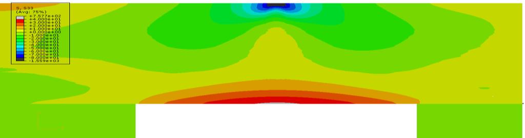
105 91 Wheel load application (a) (c) (b) (d) (e) Figure Normal stress profiles (MPa): (a) σ 1 on top view of the rail (b) σ xx contour plot on top view of the rail (c) σ yy contour plot on top view of the rail (d) σ zz contour plot on top view of the rail (e) σ zz contour plot on side view of the rail cross section through which passes the vertical plane.

106 92 The maximum von Mises stress is located a few mm below the contact surface as shown in Figure 3-22 (a). The stress profile is similar to that of profile in Figure 3-16 which means a higher deformation in this region. A few mm below the load surface at the far ends of the minor axis, is the shear stress σ xy reaches a maximum. This stress is positive at the end near the rail center and negative at the other end, as depicted in Figure 3-22 (b). Similar behavior is observed for shear stress σ yz below few mm below the elliptic load surface at the ends of major axis, as shown in Figure 3-22 (c). (a) (b) Figure Shear stresses: (a) von Mises Stress, (b) σ xy and (c) σ yz on a zoomed in rail cross-section under the load application surface area. (c)

107 Finite element for rail fatigue fracture mechanics The finite element method is also used to model cracks in the solid as a numerical technique which is usually called upon fracture problems that do not have a closed form of solution that can predict the crack initiation and propagation. Two main methods can be used: stiffness derivative virtual crack extension and energy domain integral. The virtual crack extension stiffness derivative method is discussed here whereas the continuum approach is described in [49]. The stiffness derivative formulation consists of using the energy release rate as an indicator of crack propagation and by expressing this energy release rate in terms of the finite element solution. Recall that the energy release rate is the rate of released potential energy per unit of crack advance. The potential energy itself is the energy difference between strain energy and the work done by external forces or Π = U F. Therefore the potential energy can be written in terms of the finite element solution as [49] Π = 1 2 {u}t [K][u] {u} T {F} The energy release rate is given by G = ( Π a ) = {u}t a {[K]{u} {F}} 1 2 [K] {F} {u}t {u} + {u}t a a Substituting Eq in Eq and assuming no traction forces on the crack surface, the strain energy release rate reduces to G = 1 2 {u}t [K] a {u}. 3-35

108 94 The relation in Eq indicates that the strain energy release rate is the function of the stiffness derivative with respect to the crack advance. To apply this relation a region surrounding the crack is chosen and the element stiffness matrices are assembled into one global stiffness matrix that represents the crack region only. The energy domain integral represented and derived in [49], [64], [72] has been the base of finite element formulations for fracture mechanics as an alternative to virtual crack extension. This energy domain integral is extended in three dimensions as a weighted average over a crack length ΔL as [49] J ΔL = ΔL J(η)qdη, or J ΔL = lim ro 0 S 0 [Wδ 1i σ ij u j x 1 ] qn i ds, 3-36 where J(η) is the point-wise value of J, S 0 is the surface area of the cylindrical outer counter of length ΔL and radius r o surrounding the crack tip, q is the weighting function representing the normalized crack tip advance Δa(η) such that it is zero at the crack edge and 1 at the crack outer contour, or in other words q = Δa(η) Δa max, 3-37 where Δa max is the maximum crack advance, and η is the local coordinate in the direction of the crack normal to the crack edge at a given point, W is the strain energy density function that is defined in Eq Applying the divergence theorem to Eq. 3-37, and assuming there are no thermal strains, plastic strains, or body forces the energy integral of a crack domain of volume V enclosed by two cylindrical surfaces S 0 and S 1 with radii r 0 and r 1 can be written as u j J ΔL = V (σ ij Wδ x 1i ) q dv 1 x i crack faces u j x 1 q ds. 3-38

109 95 The first term represents the domain energy integral related to the strain energy inside the volume considered, while the second term is related to the energy of traction forces on the crack faces. For the finite element implementation of the domain energy integral represented by Eq the normalized crack advance q is interpolated as a summation of the element nodal normalized crack advances weighted by their corresponding shape functions as n q = N l q l. l= Therefore, n q = N l ξ k x i ξ k x j 3 l=1 k=1 q l, 3-40 and the discretized volume J- integral is then written as m u j J = {[(σ ij Wδ x 1i ) q ] det ( x j )} 1 x i ξ k V p=1 u j w p (σ 2j q) w x f p crack faces where w p and w f are the weighting factors, m is the number of Gaussian points meaning that the quantity in { } p is evaluated at the Gaussian points. If there are no traction faces the computation over the crack surface is zero. The computation of the J- integral leads the stress intensity factors and crack propagation direction which in turn can be used in fatigue models such as Paris law to determine fatigue life. Commercial finite element codes such as Abaqus are able to handle such complicated fracture problems in three dimensions which are difficult to solve analytically because the fatigue and the crack propagation depends on the three modes of fracture. Commercial software uses the contour integral algorithm stated in Eq More details about how fracture mechanics is implemented in Abaqus are found in [71]. Malingo et al. [204] also studied this type of problem. They studied three dimensional crack growth using Abaqus and compared the results with previous experiments and found they agreed

110 96 well. Because the stresses are at the crack edge are very high, fine meshing at the crack front as the crack propagates is required. This requires very fine meshes in the entire domain where the crack will propagate therefore incurring more computational time. The technique used to alleviate this problem is to have fine meshes at the crack front, and as the crack advances remeshing is done. This remeshing can be technically problematic for the crack advancement in a complex geometric model. Moreover the crack needs to follow the elements edges which may give false results as compared with reality Extended finite element method for rail fatigue fracture mechanics The extended finite element method (XFEM) was introduced in the work of Moës et al [205]. XFEM works on a principle that the elements intersected by the crack can be enriched by specific functions thereby adding additional degrees of freedom to their nodes. The enrichment method was initiated by Belytschko and Black [206]. Further details on the enrichment method as well as work on the applicability of XFEM to model crack initiation and propagation are given in the literature [ ]. The method provides flexibility in modelling because it does not require remeshing and the crack need not follow the elements edges as requires traditional FEM. Here, XFEM allows the cracks to follow a curved path within an element. Therefore complex crack shapes such as non-planar cracks can be modelled [215], [216]. Initially XFEM was limited to cracks propagating in linear elastic materials, but recently models that use cohesive elements with XFEM have been introduced allowing the modelling of cracks of larger nonlinear elastic zone at the crack front [217], [218]. Currently XFEM has been extended to modelling crack propagation in elastic materials under dynamic loading [210]. The XFEM is currently implemented in Abaqus [219], [220]. XFEM is formulated on the basis of standard finite element displacements which are enriched by additional degrees of freedom. The elements through which the crack passes are enriched by two additional degrees of freedom at each node while elements that contain the crack tip are enriched by an additional 8 degrees of freedom on their each node. The displacement formulation in XFEM is written as [205]

111 97 u xf (x) = u i N i (x) + N i (x)h(x)a i + [N i (x) F α (r, θ)b iα ] i I i L i K α=1 The first term of the right hand side in Eq represents the classical finite element formulation of a body without a crack. The third term represents the finite element formulation of enriched elements by additional degrees of freedom a i which are multiplied by the Heaviside function; that is, H(x)=1 if x is on one side and H(x) =-1 if x is on the other side of the crack. This enrichment is specific for elements surrounding the crack faces in 3D or the crack path in 2D and excludes elements that contain the crack front or crack tips respectively in 3D or 2D. Therefore this Heaviside function allows the discontinuity of the crack to be modelled. In the third term, the elements that contain the crack tip or crack front are enriched of the nodes by 8 additional degrees of freedom b iα which multiply 4 polar functions defined by 4 F α (r, θ) = { r sin ( θ 2 ), r cos (θ 2 ), r sin (θ 2 ) sin(θ), r cos (θ 2 ) sin(θ)}, 3-43 where I is the total number of the nodes in the finite element model. L is the total number of nodes to be enriched by jump functions i.e the nodes of the elements that contain the crack path or crack surface. K is the total number of nodes that contain the crack tip or crack front. N i (x) are the usual shape functions used in classical finite element. In 2D, x can be defined by two local coordinates such that(x) = (ξ, η); where ξ is tangential axis to the crack path and η normal axis to the crack path. Therefore +1, for η > 0 H(ξ, η) = { 1, for η < 0. In 3D, x is the local coordinate vector such that x = (ξ, η, ζ). The Heaviside function is valued by signed distance to the crack faces defined by level set functions φ (ξ, η, ζ) [221] as +1, for φ(ξ, η, ζ) > 0 H(ξ, η, ζ) = { 1, for φ(ξ, η, ζ) < 0.

112 98 In Eq. 3-43, r and θ are defined as functions of signed distance to the crack surface and signed distance to the crack front as r = φ 2 (ξ, η, ζ) + ψ 2 (ξ, η, ζ) and θ = atan ( φ(ξ,η,ζ) ) where ψ(ξ, η, ζ) is the level set variable indicating the signed distance from ψ(ξ,η,ζ) the crack front [221]. Eq then is used in Eqs. 3-8, 3-9 and 3-10 in the standard finite elements. If the enrichment terms are eliminated then standard finite elements will be analyzed. If the enrichment terms remain the extended finite elements analysis will take into account the jumps conditions enrichments and crack tip enrichments in the analysis; thereby providing the means to compute the crack path and the crack propagation direction Rail crack analysis with XFEM In this section simulations for cracks in the rail are described. The rail is subjected to a vertical elliptically distributed loads with a maximum pressure of MPa at the center of the elliptic contact area and longitudinal loads of 4 MPa at the rail ends. The rail is discretized with linear hexahedral elements of 2 mm in the neighborhood of the crack and quadratic tetrahedral elements of 1 mm in the neighborhood of the elliptically distributed load. XFEM implemented in Abaqus computes the J- integrals and stress intensity factors at the static crack edge in the loaded rail. Eight contours are first investigated. It is expected that the J- Integrals converge to a stable value as the number of contours is increased. The first contour integral is defined by the smallest radius which is the enrichment radius. The enrichment radius is estimated to be equal to the element size at the top of the crack. The first example includes a rectangular crack perpendicular to the base of the rail as shown in Figure In this case, it is expected that the crack propagation is dominated by mode I fracture. This will be verified by the crack propagation directional angles as well as the values of stress intensity factors. The crack is given different initial crack lengths. The computed stress intensity factors as well J- Integrals are then compared.

113 99 Figure XFEM of the rail track section model with crack at the base of the rail. The J- integral is directly related to the energy release rate per unit area of the crack surface. Alternatively the J-integral is obtained by a contour integration of the energy englobed in a closed cylindrical ring surrounding the crack edge as described by Eq Also, as shown in Figure 3-24 (a) it is seen that the stress profile around the crack as viewed from the side of the rail, opposite which the load wheel load is applied is quite similar to the known stress configuration of a two dimensional crack [49] which can be modeled as a vertically propagating crack in a plate lying in the longitudinal plane of the rail. In Figure 3-24 (b), it is observed that the crack side which is below the load application experiences less longitudinal stresses than the other side. This is also shown in Figure 3-24 (c) where the longitudinal stress profile is widely concentrated towards the right rail base side, opposite to the rail base side below the load application. This means the crack will propagate faster when located in the offside of the load application. This is also predicted by the stress intensity factor at the crack edge, which is expected to be higher at the offside of load application than that at the crack edge side below the load.

114 100 (a) (b) (c) Figure (a) A right side view, (b) a left side view and (c) view from rail bottom of normal longitudinal stress distribution around the rail base crack. Left side is the side of load application. By the definition of the contour integration, this result should stay constant as the ring radius changes in accordance with the property of contour integration that is path

115 101 independent. However this does not happen until the ring radius is large enough because of numerical inaccuracy. Therefore the J-integral obtained from a small ring is skewed and generally has larger value because it defines the energy per unit area and there stress concentrations at the crack tip are high. As the ring becomes larger the J- integral becomes smaller until a certain value of the ring radius is attained. Above this ring radius the J- integral is expected to stay constant. As shown in Figure 3-25 and Figure 3-26, the J- integral becomes smaller along the crack edge as the contour integration radius is increased to a larger value and the values of J- integrals at the outer contours are close to each other. Also, in the middle of the crack there is a shape increase and decrease of J- integrals. The reason for this might be that at this point, there a discontinuity of opposite crack propagation directions. Figure J integral from contours 4 to 8 for a crack length a = 1 mm. The first contour has a radius of 1 mm as the element size. Contours are then equally spaced by the same distance which is equal to the first contour radius.

116 102 Figure J integral from contours 4 to 8 for a crack length a =5.0 mm. Figure J- Integral at different contours taken at crack edge point located at x = mm, where x is the lateral axis with originating from the rail vertical centerline. Also, the J- integral converges to a lower value when the radius of contour integration is increased at different crack lengths as illustrated in Figure It can be noted that the J- integral converges at contour 6 for most of crack lengths. The convergence

117 103 is seen when the J- Integral does not change as the contour number is increased. The convergence is seen at contour 6 because the J- integral on contours higher than contour 6 have a steady value as seen in Figure 3-27 which illustrates contours for a point located at ¼ rail base distance from the base side. The convergence is also achieved for cracks of lengths 2.5 mm, 4.0 mm and 6.0 mm when the J integral is taken from the midpoint of the crack edge as shown in Figure 3-28 where the J- integrals reach steady values after certain contours. Figure J- Integral of different contours taken at crack edge middle point (x = 0.0). Figure Averaged stress intensity factors over the last 5 contours for a crack length a = 4.0 mm.

118 104 The crack fracture analysis for this problem is dominated by mode I fracture. This is shown by higher K I values as compared to other mode stress intensity factors K II and K III which are very low as illustrated in Figure 3-29 and Figure 3-30 for the two different crack lengths. Note that the K I generally increases from the left side of the rail base (side of the wheel load application) to right side of the rail, keeping in mind that the load is concentrated on the left side of the rail central axis. Therefore, the right side of the crack is predicted to propagate faster than the left side. Figure Averaged stress intensity factors over the last 5 contours for a crack length a = 6.0 mm. Also, as the initiated crack increases in length, the maximum stress intensity factor increases. This result is in accordance with the basic fracture mechanics principle for a crack in two dimension under mode I which is defined by K I = σ a, where σ is the remote stress which can be approximated in this case by σ zz.

119 105 Figure The maximum averaged stress intensity factor with respect to the crack length. If mode I fatigue fracture is dominant it implies that the fatigue life can be approximately predicted using the same principles used for predicting the fatigue life of structures under uniaxial fatigue crack propagation such that K eq K I. This result can be achieved by transforming Paris law ( Eq ) as a (ΔK eq) m c N = da a 0 c Previous studies have determined the critical K eq for the pearlitte steel rail to be equal to 1100 MPa (mm). The critical crack size a c is obtained by interpolating data represented by Figure 3-30 as the crack length that corresponds to critical stress intensity factor. ΔK eq = K eqmax K eqmin. In this case K eqmin = 0 because the load varies from zero to its maximum. The utilization of the relation in Eq requires that the crack propagates in the same plane because the data used are based on cracks incremental to the same plane and actually the equivalent stress intensity is approximately the same as K I for mode I loading.

120 106 On the other hand the direction of crack propagation can be checked for the angle that shows the direction of the virtual crack advance. For a smooth crack that is propagating in one plane these angles at all points of the crack edges should be zero. This outcome is confirmed by the results shown in Figure 3-32 for angles of crack propagation directions for different lengths of the crack. The angle of crack propagation for all points varies between 3.0 o and 2.0 o almost symmetrically from left to right, the left being the side of the load application and the right being the opposite side. Figure Directions of crack propagation along the crack front for crack sizes a = 2.5 mm, a = 4.0 mm and a = 6.0 mm. At the crack edge in the rail section that lies with an interval of the lateral axis from mm to 60.0 mm the magnitude of the angle of crack propagation is less than 0.5. Also, the angle of propagation at the crack edges near the sides of the rail foot increases sharply to 3 degrees. This angle lies in the plane perpendicular to the crack front at the point considered and extending from the crack plane as is initially illustrated in Figure 2-5.

121 107 In this case it is a longitudinal plane along the rail. For positive angle the crack advance would be towards the positive z- axis (which is in the longitudinal direction of the rail) and for negative angle the crack would advance in a direction of negative z- axis, of the global coordinate system. The values of these angles are not invariant and they are slightly different along the crack edge because, as it is well known, for ductile materials, the crack fracture surface will be characterized by a rough surface. The angle of crack advances are small enough to be characterized as kinks that produce this roughness but allowing the crack to propagate in the same plane or to be self similar. This remark is also made from the dominance of K I and these angles reveal that the crack will keep propagating in the one plane meaning that the base of the rail is not affected by the multiaxial loading by the vertical load and longitudinal load. Instead, the bending stresses at the base will induce a uniaxial crack propagation at the base of the rail. 3.5 Summary In this chapter, the techniques to model the railroad track were discussed. The distributed parameter modelling was discussed. The emphasis was put on the use of FEM and XFEM to model the rail stresses and crack propagation rate as well as directions by use of examples. The principles of finite elements were discussed including element shape selection. Quadratic tetrahedral and linear hexahedral elements were chosen to be used in all FE simulations encountered in this dissertation owing to their accuracy and convergence. The modelling of the wheel in contact with the rail is very challenging because it requires very small element sizes over a large portion of the model. Therefore, it necessites very high computational time. To address this problem the wheel load was modelled as a pressure distributed over elliptical contact area using the relations derived in the literature of contact theory. Good correlation of stress distribution in a simplified model with the stress distribution n the model of the wheel in contact with the rail was observed. The simplified model is chosen to be used in the subsequent simulations. The convergence of the finite element model simulation was discussed. A global element size of 6 mm was chosen to provide converging results.

122 108 Besides the anaysis of track simulations with FE, XFEM was used to simulate rectangular cracks of different sizes perpendicular to the rail longitudinal axis. It was remarked that these cracks will propagate in the same plane. This remark was due to the fact that the stress intensity factors were dominated by mode I fracture stress intensity factor and the angle of crack propagation was close to zero. Also, the convergence of XFEM was discussed based on J- integrals at different contours. It was remarked that at least 6 contours were needed to get converging results for cracks. However a uniform track bed was considered. In the subsequent chapter, a track bed with spatial varying stiffness is considered and FEM together with XFEM is used to compute the stresses, fatigue cycles to crack initiation as well as crack propagation parameters including stress intensity factors and crack propagation angles. The selection of element shapes, sizes and the number of integration contours are based on the results obtained in this chapter.

123 109 CHAPTER 4: INFLUENCE OF SPATIAL VARIATIONS OF TRACK STIFFNESS ON RAIL STRESS AND FATIGUE LIFE 4.1 Introduction Stiffness defines the structural capacity to withstand deflections under loading. Therefore the stiffness of a structure implies how much force is required to produce one unit of deflection. The stiffness of a continuous structure can vary spatially along it. The one dimensional variation of the stiffness can be quantified as the gradient with respect to incremental distance x as k x 0. And if the stiffness varies spatially, the deflection will vary accordingly. In this section an investigation of track stiffness variation is conducted with two main aspects: 1) a study of track stiffness variation over a short distance of the rail and 2) a study of track stiffness variation within over a longer distance of the track will be studied by generating random track stiffness values in many sections of the track. In each of these studies the modellinng is done using the finite element method. The range of the track modulus is determined by comparing the FE model deflections with deflections obtained from measurements. As defined by Selig et al. [41] the track stiffness k is the defined as ratio of a concentrated vertical force, P, and the maximum deflection of the rail (δ m ), as k = P δ m. 4-1 Using Euler Bernoulli beam bending theory, and considering the assumption that the rail can be modeled as a beam supported by an elastic foundation, the equation governing the deflection is given as

124 110 EId 4 δ dx 4 = q = uδ, 4-2 where u is the track modulus, E is the rail Young s modulus of elasticity, I is the moment of inertia of the rail, and x is the horizontal distance along the rail measured from the applied load point, and q is the vertical foundation supporting force per unit length. Eq.4-2 is similar to Eq. 3-3 with a difference that the former is a concentrated load while the latter is a distributed load over a finite length of the rail. The solution to Eq. 4-2 leads to the track modulus given as [41]. u = (k)4 3 (64EI) Here k represents the stiffness of the whole track structure including the effect of the rail flexural rigidity modulus, EI, whereas the track modulus, u, represents the remainder of the track including the track fasteners and ties, ballast, slab ballast, and subgrade and therefore it excludes the effect of the rail. The relation in Eq. 4-3 represents a spatially uniform stiffness; it means, k x = Spatial variation of track stiffness and influence to train track performance The track stiffness varies both longitudinally and vertically as discussed in [23]. In the vertical direction the track stiffness is a constituent of the rail stiffness, rail pad stiffness, the crosstie stiffness, the ballast stiffness and subgrade stiffness. Also studies have shown that the track stiffness is nonlinear in the vertical direction because of the nonlinear behavior of the rail pad stiffness as well as the ballast stiffness [222]. The variations of track stiffness along the rail have been studied also by [ ]. This variation can be considered on a large scale or small scale. On the large scale the track stiffness variation is caused by, for example, the introduction of bridges, level crossings, tunnels, culverts, and switch panels. On the small scale the track variation is caused by factors such as ballast

125 111 compaction, variation of soil properties, supports under sleepers, and sleeper bays. Also research analyses have demonstrated that the stiffness is not static in the vertical direction. Rather it is dynamic and it depends on loads and time or frequency of the loads [ ]. Track stiffness and its performance on the dynamic responses of coupled train track has been extensively examined. Such studies include the work of [225] where the continuous varying dynamic stiffness along several kilometers has been measured and the studies on its effect on the dynamics of the rail and wheel rail dynamic interaction. It was found that a global low stiffness would lead to higher deflections of the rail, thereby increasing the bending moments while global stiffness would lead to higher wheel rail interaction forces which increases stresses at the wheel rail contact interface. Although the findings indicated that the track stiffness varies along the track, the extent to which the spatial stiffness variation would affect either the rail integrity or the dynamics of both rail and the train was not investigated. Studies to investigate the effect of track stiffness on the speed of the train and train vibrations have been done using discrete finite element [229]. Also a similar study was conducted in [230] which investigated the effects of track irregularities and the spatial stiffness variation were investigated. It was argued that spatial variation of stiffness has an effect on parametric excitation of the rail car but not to the extent that the track irregularities do, according to their calculations and measurements. The works done in [162], [223], [225], [227], [231] show that the spatial stiffness variation increases the wheel rail contact forces. Therefore the rail surface deteriorates due to high stresses developed at the contact interface. On the other hand when it comes to predicting the rail fatigue life, researchers assume a track bed of uniform average modulus to describe cyclic stresses and bending moments developed in the rail as well as rail for crack growth problems [1], [197], [198], [ ] and also to study the fatigue life of the railroad bridges. The rail fatigue life studied in previous work is therefore based on fatigue crack growth which depends on loads acting on the rail, temperature, and residual stresses found in rail after manufacture or temperature increase by welding.

126 112 The work presented in this chapter is focused on the influence of spatial track stiffness variation to the track fatigue life and crack initiation. Preliminarily, the relation between the statistics of track stiffness on the rail stresses is studied. The crosstie Young s modulus is used as the parameter that models the track support modulus. This approach is achieved by comparing the example measurements of rail vertical deflection with the rail deflection given by the finite element analysis. The crosstie modulus that yields the rail deflection in finite element method in same range of the rail deflections is chosen as the crosstie modulus that represents the total track support. The details of measurement technology utilized by MRail, Inc can be found in [44] and are reviewed in the next section. Different cases of track models and track modulus variations are considered to quantify the tangible effects of track stiffness variation to the damage of the rail. A short model of the track which consists of a single rail, a middle crosstie and two half side crossties is used to estimate the crosstie Young s modulus that, under given boundary conditions, would give the same rail deflection as rail deflections measured in the field under real loads. The track geometric model in this case is studied with periodic boundary conditions and the results are compared with the model of free ends. Then, the ratio of the side crosstie stiffness with respect to the middle crosstie is varied and the influence of the stiffness variation to the rail stresses is investigated. In this case the rail has free ends and the crossties are fixed on the bottom. The side crossties are given periodic boundary conditions on far end sides. Lastly, a long track model composed of a single geometrically simplified rail with rectangular cross section, ten crossties fixed at the bottom, and periodic boundary conditions applied at both ends of the rail is used. The stiffness of the track is considered to be random with an average modulus in the crossties and two statistical cases: first, by fixing the standard deviation of the moduli and varying the moduli average around the modulus that represent the total track support modulus. Second, the moduli standard deviation is varied and the moduli mean is fixed. Both types of stiffness statistics are used to compute the statistics of the stresses in the rail. The statistics of cyclic stresses at a given point in the rail within the context of cyclic loading can be used to determine the number

127 113 of cycles to crack initiation using a multiaxial fatigue model, and the stress intensity factor ranges for fatigue crack propagation rate. 4.3 Measurement of track stiffness, modulus and deflection Possible maintenance issues associated with the railroad track can be identified by measurement of the track stiffness. The measured track stiffness is compared with the desired track stiffness [22], [237] for healthy railroad track. For evaluation of track performance, the optimal track stiffness is a necessary parameter to take into consideration. When the stiffness is too low it results in a large deflection of the rail while a high stiffness causes large wheel rail interaction forces and induces high stresses at the contact interface of the wheels and rail [223], [228]. Therefore by measuring the track stiffness railway engineers can decide whether to replace the rail or to rehabilitate the track substructure and superstructure components. Different measurements methods are available. They can be static or dynamic measurements. Static measurements rely on static loads and track deflection relationships. The track stiffness obtained in this case is assumed to be independent of the railcar speed. Dynamic measurements consist of obtaining the relationship of track deflections under a moving load. The stiffness obtained in a dynamic measurement is a function of moving load speed and therefore as a function of excitation frequency. This excitation frequency is normally due to irregularities on track causing load impacts Static measurements Early static measurements as described in [41] are: deflection basin test, single load point test, multiple axle vehicle load test, and computation from track model. The deflection basin method is based on the equilibrium of vertical forces acting on the track which includes railcar loads acting on the rail through wheels P j and the track resistance forces. The track resistance forces are determined by measuring the crosstie deflections δ i normalized by a length S. If the track modulus defines the modulus per unit of track

128 114 longitudinal length per unit vertical distance down deep into the track, from the equilibrium equation, the modulus can be deduced as u = S n j=1 P j m i=1 δ i. 4-4 where S is the center to center crosstie spacing, n is the number of the wheels and m is the number of crossties that are deflecting under the vertical loads. The relation in Eq. 4-4 assumes a linear load and deflection relationship. However the track load and the deflection relationship is not really linear. Therefore a better approximation can be obtained by computing the modulus from the incremental loads and the incremental crosstie deflection relationship which is u = n j=1 (P h P h 1 ) j S m ( δ h δ h 1 ). 4-5 i=1 i The single load test is an easier way of estimating local track modulus. The modulus estimated using the deflection basin method requires measurements of crosstie deflections over a very long distance. The single load test considers only the load from a single wheel and will uses the relations in Eq. 4-1 and Eq. 4-3 respectively to estimate the vertical track stiffness and track modulus. To account the nonlinearities, the track stiffness, as a function of the load, is computed as a ratio of load change to rail deflection change. The multiple axle vehicle test uses the railcar with two or three axle trucks for loading and the deflection basin method can be used to estimate the track modulus. On the other hand computer models [238] can be used to superpose the rail deflections from loadings of two axle bogies. The computation from track model uses a computer program such as GEOTRACK [238] to predict the effect of different parameters in the track on track stiffness and modulus. In the case considered in this chapter, a computer model with static loads is developed.

129 Dynamic measurements of track stiffness and deflections Dynamic measurements are a more accurate representation of the track modulus under given loading conditions as it has been demonstrated that the track modulus is influenced by different dynamic parameters including the railcar speed and load excitation frequency. Therefore the dynamic measurement of the stiffness is specific to a certain range of railcar speed as well as excitation frequencies. For example, the rail deflections under high railcar speeds can be accomplished by high speed deflectograph [239], [240] which measures the rail deflection velocity under high speed travelling railcar using a number of laser sensors mounted on a beam positioned in front of one of the wheels. One sensor is placed at the far end of the beam away from the wheel acting as the reference as it is directly positioned above the undeformed rail. The other sensors are mounted on the same beam in the proximity of the wheel and register the rail deflection velocity. This technique has also been extended to measure the vertical deformation velocity of a road under higher driving speed [241]. Another measurement technique based on track deflection velocity measurement to evaluate dynamic track modulus from the speed of moving load has been carried out in the work described in [242] where geophones are used and placed at the crosstie locations. The oscillation speed of the moving track when the train passes is recorded by the geophones and this signal can be converted into track modulus by applying the deflection basin test method as well as modified beam on elastic foundation. The shortcoming of this method is that the continuous modulus over very long distance cannot be measured. Another technique to measure the track dynamic global stiffness is introduced in [237] where a Rolling Stiffness Measurement Vehicle consisting of a two axle wagon is equipped with a loading mass and measurement tools consisting of force transducers and accelerometers. The track is then excited by two oscillating masses and the track stiffness is calculated from the measured oscillating force and acceleration as a complex value with the magnitude being a function of oscillating frequency. The drawback of this technique is that the real track stiffness under full train loading cannot be measured.

130 116 Another technique to measure the track modulus based on vertical deflection measurement has been developed at the University of Nebraska and the details pertaining to the design, instrumentation and operations for railroad maintenance are given in [43], [44], [46]. It is based on coupled camera laser sensors mounted on a beam positioned in front of the train truck wheels. The measurement technique consists of two laser sensors and a camera as shown in Figure 4-1 (a) and (b). The camera is placed between the two laser sensors at distances L 1 and L 2 from each laser sensor. Camera and laser sensors are placed horizontally at height H from the undeflected rail. When the rail deflects under loading of wheel, for a distance y w the vertical position of the camera from the undeflected rail surface becomes h; on the other hand this position is not truly the position from zero rail deflection as shown in Figure 4-1 (a) as at that horizontal distance the rail has some small deflection represented by y c. The laser light is emitted at angles θ 1 and θ 2 crossing each other before they reach the rail surface. The laser light therefore make a light spot pattern on the rail surface, an image that is taken by the camera. The width of this light spot pattern on the top surface of rail is represented by distance d on Figure 4-1 (b). This width can be determined by analyzing the camera image using a computer program. Knowing the measurement of d, and because L 1 and L 2, and the angles θ 1 and θ 2 are known, the relative vertical deflection of the rail from the position of the rail top surface can be determined and is given by [43] y r = H h = H d + (L 1 + L 2 ) 1 tan θ tan θ 2 4-6

131 117 (a) (b) (c) Figure 4-1. (a) and (b) Schematic diagram of UNL equipment working principle for vertical track deflection measurement (regenerated from [43]). (c) Instrumentation and location of rail deflection measurement equipment [44]. Example measurements of the rail deflection measurement are shown in Figure 4-2. As it is demonstrated in Figure 4-1 the relative deflection represents how much the rail has deflected at the point of rail surface contact with the wheel relative to the deflection of the rail top surface below the camera. The positive data therefore means that there is a

132 118 deflection; but, as shown in Figure 4-2 measurement data have an oscillatory pattern along the rail and this oscillatory pattern includes negative measurement data. The negative measurement data therefore mean either that the rail at the contact with the wheel has jumped upward or the wheel has lost a contact with the rail due to train vibration. Figure 4-2. Relative deflection measurement data of the rails (Courtesy of MRail,Inc [243]). The rail deflecting upward would mean that the rail top surface which is being measured is already in vibratory motion which has been initiated earlier such that the wheel tends to follow this motion. Also, it can be pointed that the measurements are affected by different factors as discussed in [43], [44], [46], [244] including the train kinematics such as pitch motion and the rail geometry irregularities. These measurements will be used to estimate the modulus of the crossties supporting the rail in the finite element models used here. Because the negative deflections do not reflect the track modulus, only positive measured deflections are used to compare the track deflections given by the finite element model. Initially the averages of relative track deflections represented by positive values at different sections of the track are calculated.

133 119 The track is divided into different intervals as shown in Table 4-1 and these averages range from 2.0 to 3.5 mm. Table 4-1. Average relative deflections of the track at different section (Courtesy of MRail,Inc). Interval Intervals in m Average deflection in mm Number Start point End point Left rail Right rail Track modulus statistics and their impact on track fatigue life In this section the impact of spatial variation of the track support modulus on the cyclic stresses generated by repeated loadings from the train wheel is studied using finite element method. Field measurements are used to determine the range of crosstie modulus of the models. The model consists of a single rail that lies on three crossties, extends between center to center of the side crossties and has a length of mm. The cross-section dimensions of the rail and longitudinal section view of the crosstie are shown in Figure 4-3 (a) and (b).

134 120 (a) (b) Figure 4-3 (a) The dimensions of the rail half cross section in mm, (b) The dimensions of the crosstie section in mm. The crossties are given fixed boundary conditions at the bottom. The crosstie Young s modulus represents the total track bed modulus that would yield the same track deflection in the real situation of a track under a running railcar. Therefore, for the model

135 121 of the track a support modulus which gives a deflection that falls in the range of 1.0 mm and 4.0 mm is needed. The same model geometry is used in [245] but in their work the wheel rail contact surface area is assumed rectangular. Here, the same loading as shown in Figure 3-17 is used for which the wheel in contact with the rail results in an elliptically distributed load on the rail top surface. The load is also applied eccentrically on the rail with the load center is offset by 14.8 mm from the rail vertical mid plane. After substituting in numerical values in Eq , this loading is represented by σ y y (z, x ) = MPa 1 z 2 (9.2mm) 2 x 2 (7.8mm) 2, 4-7 which is distributed at the elliptic contact surface area defined by z 2 (9.2mm) 2 + x 2 (7.8mm) 2 = 1, 4-8 where, x, y, z are the local coordinate axes having origin shown in Figure 4-4. The center of the ellipse of load application is defined by axes z 1 = 9.2 mm, and x 1 = 7.8 mm such that x = x 14.8 mm, y = y mm and z = z mm. The global coordinate system has origin at the right side base edge center of the rail section as shown in Figure 4-5 and Figure 4-6, if it is extended to full length of mm and has similar orientation as the coordinate system shown at the left hand side of Figure 4-4. The mechanical properties of the rail consist of a Young modulus of 200 GPa and a Poisson s ratio of 0.3. The model is repeatedly run with Abaqus with different crosstie moduli and a relationship between the deflection and crosstie modulus is established.

136 122 y z x Figure 4-4. Rail contact patch area for wheel load application and its local coordinate system. Appropriate finite element shapes, element types, and element sizes are chosen according to the accuracy needed to be achieved. For example, a global element of 6 mm is used to yield a good solution convergence. An element size of 1 mm is used the region that has the surface area of load application. Quadratic tetra hexahedral elements are used in this region because the elliptic distribution of the load is applied. The remaining section uses linear hexahedral elements. As discussed in Section both types of elements, quadratic tetrahedral elements and linear hexahedral elements, yield the same accuracy of solution but can be used differently depending on the geometry of the model. Also, the former takes slightly higher computer power than the latter. The former is used for complex geometry and the latter suits the simple geometry well. The boundary conditions are such that the crossties are fixed at the bottom as represented in Figure 4-5. The relation in Eq. 4-7 is used to add the vertical loading condition whereas a longitudinal tensile load of 4 kn is used as represented in Figure 4-5. This load comes from the findings of longitudinal loads in rail in [239]. For one case, periodic boundary conditions are applied at end sides of the side crossties and the rail end sides are unconstrained as it is represented in Figure 4-6. In another case, periodic

137 123 displacement constraint boundary conditions are applied as shown in Figure 4-7. In both cases, the rail and the crossties are tied together. Figure 4-5. Boundary conditions: Displacement constraints and load applications on the model. y L x Figure 4-6. Displacement constraint conditions, a case with unconstrained displacements at the rail end sides. L=533.4 mm.

138 124 Figure 4-7. Displacement constraint conditions, a case with periodic displacement constraint conditions at the rail end sides. The maximum vertical displacement solution in both cases is compared. Therefore if it is noticed that both cases yield close vertical deflections of the rail the first case will be preferred for further analysis. The periodic displacement constraints in this problem define boundary conditions of the rail such that both ends of the rail behave as if they are connected. Simply, referring to Figure 4-6 or Figure 4-7 these constraints can be represented by u(x, y, 0) = u(x, y, L), 4-9 v(x, y, 0) = v(x, y, L), and 4-10 w(x, y, L) w(x, y, 0) = L, 4-11 where u, v and w are displacements components respectively in x, y and z directions. These conditions are applied on CAE models through programming scripts detailed in Appendices B and D.

139 125 Figure 4-8. Rail vertical deflection profile with free ends boundary conditions. The comparisons of rail vertical deflections for the two models, one with free ends boundary conditions and another with periodic boundary conditions at the ends indicates that the maximum deflection achieved for both models are almost the same with a negligible difference of 4 %. The model with free ends achieves a highest deflection of 3.3 mm while the periodic boundary conditions based rail model that achieves a deflection of 3.16 mm. However the deformation is quite different as shown by the contour plots of deflections in Figure 4-8 and Figure 4-9. On the other hand this difference does not affect the results very much the results when choosing only the maximum values. For simplicity and computer power efficiency the model with free ends is chosen to be used for the next studies because of the need to run several models such that computer time is saved.

140 126 Figure 4-9. Rail vertical deflection profile with periodic boundary conditions at the ends Uniform and nonuniform track support modulus The FE model is first used to calculate the deflection as a function of support modulus assuming a uniform track bed. The relationship between the rail deflection and spatially uniform crosstie modulus is established. It is found that this relationship exhibits the monotonically decreasing behavior as shown in Figure This result means a slight decrease of the uniform modulus will lead to an increase in the rail deflection. However if the modulus is very high a further increase will not change anything on the rail deflection significantly. The data points are fit by the equation y r = E E 2, 4-12 where y r is the maximum rail deflection in mm and E is the crosstie Young modulus in MPa, which allows the resulting deflection for a given modulus to be estimated. The maximum principal stress profile around the rail is depicted in Figure The highest maximum principal stress in the rail is found to be located in the proximity of the load application.

141 127 Figure Deflection versus crosstie moduli relationship. A similar behavior to the modulus deflection curve is observed in the relationship of maximum principal stress versus the uniform crosstie Young s modulus as shown in Figure However, although the trend is similar the stress changes within a small range. For example a reduction in modulus from 1000 MPa to 200 MPa yields a change of approximately 0.6 MPa which is less than 0.3% of stress increase. This result shows that an increase in the average modulus for a uniform track bed does not significantly change the stresses in the rail or the fatigue life of the rail at the considered section even if the rail deflection is high. Similar behavior can be observed for other stresses. But in case of von Mises stresses the trend is in the opposite direction; an increase of the track modulus leads to an increase of von Mises stresses.

142 128 Figure Maximum principal stress fringes on the model. Figure Relationship of maximum principal stresses with respect to crosstie moduli variation for a uniform track bed. As illustrated in Figure 4-13 the von Mises stress increases slightly as the modulus increases. This outcome is because a stiffer track support results in higher deformations near the load application. Note that the von Mises stress is related to the deviatoric stress

143 129 tensor which indicates how much deformation has occurred. It is also noticed that other stress tensor components, as plotted in Figure 4-14, change very slightly over a wide span of change of uniform track modulus. There exists an optimum track support modulus below which rail stress increases due to bending and above which other factors to induce wheel rail surface interaction stresses are more important. The deteriorating effect of the track bed that is too stiff is beyond the scope of this dissertation. Figure Relationship of von Mises stress with respect to crosstie moduli. Also, if a significant decrease in modulus leads to significantly increased rail deflection and slightly increased maximum principal stress it implies that a significant increase in rail deflection should lead to a slight increase in maximum stress which ca be seen in Figure The basic idea behind this phenomenon is that under uniform track modulus there will be less change in bending moment in the rail as the modulus is changed.

144 130 Figure Some of the stress tensor components with respect to crosstie modulus. Figure Deflection relationship with respect to maximum stresses in the rail under varying uniform track support modulus ranging from 200 MPa to 300MPa.

145 131 After determining the crosstie modulus range for the finite element model, the impact of the variation of the modulus in the two successive crossties on the maximum stresses in the rail is studied by repetitively running the FE code parameterized by the ratio of the middle crosstie modulus and the side crosstie modulus. The uneven track support can be represented using different Young moduli of neighboring crossties, one as a ratio of the other. This procedure gave information about how a localized sudden change of track support modulus can affect the fatigue life of the rail while changing the magnitude of the maximum cyclic stresses in the rail. The maximum crosstie modulus is set to be 500 MPa. In this model stresses are analyzed against the ratio of the modulus of the middle crosstie to the modulus of the neighboring crosstie. As shown in Figure 4-16 the maximum principal stress, σ 1 increases significantly as this ratio increases or decreases. The minimum of the maximum principal stress occurs when the ratio is 1. This stress varies from 375 MPa to 610 MPa when the modulus ratio changes from 1 to 8. This change in stress is very significant which implies that if there is an abrupt deterioration of track support foundation it can result in a very fast degradation of the rail if there is an initial defect such as a crack. The same trend is also observed on the rail vertical deflection versus track moduli ratio as shown in Figure The deflection is a minimum for a ratio of 1 and increases to 5.5 mm for a ratio of 8 mm.

146 132 Figure Relationship of rail maximum principal stress with respect to the ratio of crosstie moduli. Figure Relationship of maximum principal stresses with respect to the ratio of the crosstie moduli variation.

147 133 Figure Component of the stress tensor as the stiffness ratio in the crossties varies. The variation of crosstie modulus affects only the normal stresses and will not affect the shear stresses as indicated in Figure This result is mainly because the uneven track support modulus induces additional bending moments in the rail and these bending moments affect only the normal stresses and not the shear stresses. A similar result is observed when the modulus is uniform and whether it is increased or reduced the shear stress stays nearly constant Long track section with randomly distributed track support moduli Now that the influence of localized modulus variation is known the next step is to see how spatial variations in standard deviations and averages of randomly distributed track support moduli influence the maximum stresses in the rail thereby changing the fatigue life of the track. Such an approach is not currently used in other fatigue models for maintenance scheduling. To achieve this goal, a long track across a set of many crossties is needed to represent the statistics of track stiffness. In the case considered here 20 crossties are selected to represent a typical rail that spans the length of two railcars.

148 134 Such a model can be computationally expensive such that geometric simplification is used to eliminate the need of small elements. It is assumed that the rail has a rectangular cross section with same cross section area as the actual rail. The calculations resulted in a cross section area of 73 mm width and 186 mm height. The rail has a length of m. The center to center distance between two neighboring crossties is mm. The crossties have the same dimensions as in the previous section, a height of mm, a width of mm and a length of mm. It is assumed that the load applied on this rectangular beam from the wheel is of uniform pressure with the same total force magnitude as 1/8 th of the total railcar static weight because one railcar has 8 wheels. The load of 142 kn is applied at a rectangular surface area. This load is in the same range that is usually used in simulation of the rail loading with FE by other researchers [153], [222], [239]. Periodic boundary conditions are applied at the end of the rail. The contact pressure distribution described earlier by Eq and Eq is applied on a rectangular surface with same area as the elliptic surface for a realistic wheel-rail contact. The area of the elliptic contact surface is given by A c = πz 1 x 1, 4-13 where z 1 and x 1 are respectively the major and minor semi axes of the elliptic contact area between the railcar wheel and the rail. The pressure applied to the rail with rectangular geometry is the average of the pressure distribution on the wheel-rail elliptic contact surface area and is given by P v = 1 A c P c (z, y)dzdx 4-14 x 1 z 1 1 x2 x 1 2 = 1 σ πz 1 x max 1 z2 2 1 z x2 2 1 x 1 x 1 z 1 1 x2 x2 1 dzdx, P v = 2σ max

149 135 w p = πz 1 x 1 /w r 2z 1 2x 1 w r Figure The rail geometric simplification for the long rail model with rectangular cross-section and rectangular surface of load application. This pressure is applied over a rectangular surface area. The width of the surface area across the top surface of the rail is equal to the width of the rail w r and therefore the width of this area is given by w p = πz 1 x 1 /w r as shown in Figure Another stipulation for this model is that the load is applied only on rail section positions located in the middle of the two neighboring crossties. Also, the crossties have constrained displacements as the boundary conditions at the bottom. The rail has periodic constraints for displacements represented by Eqs.4-9, 4-10 and 4-11 where L = m. This model accounts multiple railcars with each rail car having this length such that at every distance L there is similar loading on the rail and therefore causing similar displacement constraints. Although this is not exactly accurate the results should be much more approximate to the real conditions.

150 136 The crosstie moduli are generated randomly as chosen from a pool of data with a Gaussian distribution having the chosen mean and standard deviation. The crosstie moduli means are chosen to be below 500 MPa which means a maximum vertical rail deflection above 1.0 mm as it is computed for the short track model. A single run of the model then includes a long track with a static load at a given position and random crosstie moduli at a given average and standard deviation. The load is moved to different positions on the rail to constitute a complete realization of the model at fixed crosstie moduli mean and standard deviation. Each realization is repeated multiple times. In the case considered here it is repeated 5 times. Afterwards, the moduli standard deviation is incremented and at each increment the process of realization is made and repeated. The moduli standard deviation is incremented up to a certain number of realizations to complete a whole Gaussian simulation (same mean and different standard deviations). The mean can be changed in order to perform a different Gaussian simulation. A complete simulation consists of multiple Gaussian simulations each having a different mean. The random crosstie moduli are selected from a pool of Gaussian distribution with a chosen mean and standard deviation (SD). The resulting average and standard deviation of the 20 values is not exactly equal to that of the input distribution because of the finite number of values. This problem is remediated in two different ways and the results are compared. In the first case, for each standard deviation 19 models are created. Then multiple realizations of these 19 models with the same mean and standard deviation are repeated up to 5 times. 6 increments on standard deviations are done. The means are varied 3 times. Therefore 1710 models are run. Basically, this led to increased memory capacity, but, the models could be simulated separately therefore allowing easy management of memory. In the second case, a set of 20 random crosstie moduli are picked and these numbers are perturbed to give the same average and standard deviation as the requested mean and standard deviation of the pool of infinite data. This method is very beneficial because the perturbed numbers are still Gaussian distributed and there is no need to repeat. Thus, the

151 137 memory required in comparison with the previous case is reduced by 5 times because 342 models are run instead of 1710 models. Examples of Gaussian distribution of track support moduli, for the first case are shown in Figure For these 4 examples it is shown that as the requested standard deviation is high (in this case the highest requested standard deviation is 100 MPa and it is represented by curves with lower peaks in Figure 4-20) the higher is the perturbation of the average from the requested mean. For instance for the random numbers requested in the Gaussian data pool exhibiting the standard deviation of 100 MPa and mean of 250 MPa, it respectively resulted in averages of MPa and MPa while a lower standard deviation of 40 MPa both means resulted sample averages of MPa and MPa. Figure 4-20 also highlights the probability density of numbers close to the mean in an interval bounded by points E 1 and E 2 where both Gaussian distribution curves cross each other. If the standard deviation of the moduli population increases from σ E1 to σ E2 keeping the mean the same, the probability density, decreases while this probability density of numbers far away from the mean or outside this interval will increase. That is why a request of a sample of numbers with high standard deviation returns a sample that has an average different from the mean of the Gaussian distribution from which the sample is requested.

152 138 (a) Figure Gaussian distribution curves for some examples of randomly distributed crosstie moduli with a mean of: (a) 200 MPa and (b) 250 MPa. Oval points indicate numbers picked from data pool with a SD of 100 MPa and diamond points indicate numbers from a data pool with a SD of 40 MPa. (b)

153 139 Correcting random track moduli to yield given average and standard deviation The simulations used different samples with each having 20 crosstie moduli of the pool of many numbers of same mean and standard deviation. Each sample is used in the simulation and the samples are as many as 5 so that the resulting average and standard deviation of 5 samples is as close as the mean and standard deviation of the pool. However it is found that the resulting averages are off and the difference tends to increase as the standard deviation increases. For an additional simulation, a set of 20 random track moduli are tried in a single realization for each mean and SD such that the statistics are based on a set of 20 data. Each realization, of 20 runs, is repeated for a number of SD increments and then the whole process is repeated for different means. The random set of values selected is first perturbed so that its average and standard deviation (which in this case is taken as square root of the second moment about the mean) are the same as the mean and standard deviation of the pool of Gaussian data distribution. To do this suppose each data set carries N numbers representing the crosstie moduli. Let also X i represent each individual data point in the set of numbers. Let μ be the mean of the pool of Gaussian data distribution at given standard deviation σ. If the μ x and σ x are the average and standard deviation of the sample data set, we want to perturb X i to X i such that the new data set will have a new average μ x = μ and standard deviation σ x = σ. To get started, the average of the data set is expressed as μ x = N i=1 X i N, 4-16 Therefore the new data in the sample that gives the same average as the population mean can be perturbed as X i = X i + μ μ x, for i = 1, 2, N The second moment about the mean (variance) in the new sample can be written as

154 140 σ 2 x = N X i 2 i=1 N μ Note that N is the normalization because the mean is not included in the sample. In other words the probability for the mean of infinity numbers to be in the sample is almost zero. Because changing the sample elements will change its standard deviation the sample elements must be perturbed again such that its mean does not change but the standard deviation becomes σ. To achieve this a perturbation number is added to the elements on the left of the sample median and subtracted from the elements which are on the right of the sample median. Therefore the elements need to be ordered from the smallest to largest so that the variance can be written as N/2 σ 2 = (X n + c) 2 + n=1 N (X n c) 2 n= N 2 +1 μ 2, 4-19 where X 1 X 2 X n 1 X n X n+1 X N 1 X N. Subtracting Eq from Eq gives N 2 Δ σ 2 = (X n + c) 2 + n=1 N (X n c) 2 n= N 2 +1 N 2 i=1 X i N, 4-20 where Δ σ 2 = σ 2 σ 2 x. Expanding the terms in parentheses on the right hand side of Eq and performing algebraic manipulation gives N/2 N X n c X n c + nc 2 nδ σ2 = 0, n=1 n= N This expression can be also written as c Δ μ x c Δ σ 2 = 0, 4-22 N N 2 n=1. where Δ μx = X n= N n X 2 +1 n

155 141 From Eq. 4-22, c can be found as c = 1 2 Δ μ x 1 2 Δ μ 2 x + 4Δ σ Note that the other value of c is disregarded because it would result in negative elements of the perturbed sample. The new sample has the following elements X i = X i + μ μ x + c for X i < X med, and X i = X i + μ μ x c for X i > X med, 4-24 where X med = 1 2 (Xn 2 + Xn 2 +1 ). n=n Therefore the algorithm that randomly chooses a set of data in a pool of data with a given mean and standard deviation is extended to include Eq This new algorithm that implements this adjustment has to include certain constraints such as Δ 2 μx + 4Δ σ 2 0 and X i > X lb where X lb is a chosen minimum value (lower bound) that is allowed to be in a set. For example, negative numbers cannot be allowed in the set. Also, a constraint on the upper bound can be added, such that the modulus cannot be above a certain chosen limit. If the set of data does not meet these constraints then the set is rejected and another set of data is randomly chosen until all constraints are met. Gaussian distribution of randomly generated track moduli in a single realization Four example sets of track moduli can be represented on Gaussian distribution curves as shown in Figure One thing to notice is that the sets with higher standard deviation keeps the Gaussian distribution behavior but the data with less standard deviation seem to have a disturbed Gaussian distribution. These sets of track support moduli have exactly the statistics requested. A constraint 20 MPa as the minimum value of data in each set is applied. Another thing to realize is that as the standard deviation increases it implies many fluctuations in the data meaning that we have very small values and very large values. In reality, it is not very common when to have a track that has large fluctuation track support moduli variations. Therefore the results which are inherent to lower standard deviation can be more important as they could relate to reality.

156 142 Figure 4-21 Examples of Gaussian distribution of crosstie moduli. In the following section a study of the influence of the track support moduli statistics on stresses, particularly principal stresses and bending stresses (longitudinal stresses) and deflections is made. In the first case the stresses and deflections as functions of variation of the mean of track support moduli are studied. In the second case the stresses and deflections as functions of varying standard deviation of the track support moduli are investigated. 4.5 Computed results for long track model In this section the results of stresses and fatigue cycles in a long track with randomly varying track modulus are provided. The study compares the stresses and the fatigue cycles in the rail supported by randomly varying modulus at different means and fixed standard deviation. Then, the stresses and fatigue cycles to crack initiation in the rail of a track supported by randomly varying track modulus at different standard deviations and mean are computed. The final study looks at the impact of track modulus variation on the crack propagation rate.

157 Variation of mean track modulus This section consists on computing maximum stresses each time the load is applied at any of the 19 positions that are chosen separated by equal intervals and their averages over all positions at a fixed mean and Standard Deviation (SD) of random track support moduli. The track moduli mean is incremented from 100 to 550 MPa in increments of 50 MPa all with the same SD of track support moduli. Therefore a total of 190 code runs are performed and 190 output databases are analyzed by scripting and programming to extract and manipulate the data. The contours of maximum principal stress for three examples both at a mean of 100 MPa and a SD of 60 MPa but for different positions of the load applications are shown in Figure 4-22, Figure 4-23, and Figure As expected the stresses are compressive on the top while tensile at the bottom of the rail model. Figure A model that has average track moduli of 100 MPa, at a SD of 60 MPa and the load at position 1.

158 144 Figure A model that has average track moduli of 100 MPa, at a SD of 60 MPa and the load at position 2. Figure A model that has average track moduli of 100 MPa, at a SD of 60 MPa and the load at position 9. The resulus from the analysis are given in terms of deflection and stress. As the modulus average increases the average deflection in the rail decreases as shown in Figure 4-25 (a) and (b). The average of the highest maximum principal stresses as well as the average of the highest maximum principal stresses in the rail decrease as the average modulus in the crossties increases, as illustrated respectively in Figure 4-26 (a) and (b). Note that the trend of the curve that illutrates the variation of principal stresses with respect to the variation of track moduli (Figure 4-26 (a) and (b) ) is similar to the trend of the curve of the variation of deflections with respect to the track support moduli variation (Figure 4-25 (a) and (b)). This result confirms that the stress and deflection have a linear relationship as already observed in Figure 4-15.

159 145 (a) (b) Figure Relationship of the rail deflections with respect to the rail deflections average crosstie moduli.

160 146 (a) Figure Relationship of the maximum stresses with respect to average crosstie moduli. (b)

161 147 The directions of the maximum principal stresses are found to be dominated by longitidinal directions which means the highest stresses in the rail are longitudinal tensile or compressive stresses. These directions are tabulated in Table 4-2, for the case of average track support moduli of 150 MPa, as cosines of the angles between the normal to the principal plane and the coordinate axes. Therefore α is the angle between the normal and x axis, β is the angle between the normal and the y axis and γ is the angle between the normal and the z axis. It is observed that the cosines of γ are close to one while the cosines of α and β are close to zero. This result means that the resulting unit vector is close to z- axis and thererore the maximum stresses have a longitudinal direction. Table 4-2. Maximum principal stresses and their principal plane normal directions for crosstie moduli with a mean of 150 MPa and a SD of 60 MPa. Crosstie No σ 1 (MPa) cos α cos β cos γ E E E E E E E E E E E E E E E E E E E E E

162 Influence of varying standard deviation of track support modulus Figure 4-27, Figure 4-28, Figure 4-29, and Figure 4-30 show examples for the resulting maximum deflections at each load position shift with a change in standard deviation of the track support moduli with a mean of 250 MPa. For example for a standard deviation of 22 MPa as shown in Figure 4-30 the maximum deflections is around 1.68 mm and when the standard deviation increases to 60 MPa as shown in Figure 4-29 the maximum deflections increased to around 1.9 mm. For a standard deviation of 74 MPa, the maximum deflection increased to about 2.2 mm as shown in Figure However, an increase in standard deviation to 95 MPa resulted in decrease of maximum deflection to around 1.65 mm. This result can be explained by probabilistic phenomena. As the standard deviation increases the random numbers selected are more likely to be far away from the mean, or in other words the probability to randomly choose numbers far away from the mean is higher than before the standard deviation is increased. In this case if there are more track moduli which are far away from the mean and they are close to each other, although they may be smaller but the fact that their difference is small will lead to less deflection because the ratio of those moduli is small according to the illustration in Figure Another way to explain this is that as the standard deviation becomes higher, the track is likely to have very high crosstie moduli which have a larger difference; but, as shown in Figure 4-10, higher track moduli lead to less deflections even if their differences are large.

163 149 Figure Maximum deflections at different load positions under random track support moduli with a mean of 250 MPa and standard deviation (SD) of 96 MPa, first trial of the realization. However, if we continue multiple repetitions of a realization, maximum deflections will likely be high at increased standard deviation. In this case 5 repetition of each realization are made. As a result the overall deflection in 5 trials at moduli standard deviation of 100 MPa is increased. Keeping in mind that the results presented in the Figure 4-27, Figure 4-28, Figure 4-29, and Figure 4-30 are for one of 5 repeated realizations, it is expected that the maximum deflection increases with increased standard deviation after a sufficient number of realization repetitions is completed for each SD. It will be shown that the overall longitudinal stress at this SD is higher than the one obtained for a SD of 80 MPa. Note that not only the maximum deflections increased but also the minimum deflections decreased as the standard deviation increased. For example, the highest minimum deflection occurred for a moduli standard deviation of 20 MPa is 1.53 mm, as shown in Figure 4-30, and is reduced to the lowest minimum deflection of 1.2 mm when the track moduli standard deviation become 100 MPa, as shown in Figure 4-27.

164 150 Figure Maximum deflections at different load positions under random track support moduli with a mean of 250 MPa and standard deviation of 74 MPa, first trial. Figure Maximum deflections at different load positions under random track support moduli with a mean of 250 MPa and standard deviation of 60 MPa, first trial.

165 151 Figure Maximum deflections at different load positions under random track support moduli with a mean of 250 MPa and standard deviation of 22 MPa, first trial. The maximum bending stress tends to follow the same trend as the maximum deflections in the rail. This result can be confirmed by comparing, for instance, the results represented in Figure 4-27 and Figure Also, the maximum principal stress increases as the standard deviation of the track support moduli increases except when the standard deviation (SD) of the moduli is 100 MPa. These remarks are based on the results shown in Figure 4-31, Figure 4-32, Figure 4-33, and Figure To get the increased longitudinal stress at higher standard deviation more trials are needed. Therefore, as shown in Figure 4-35 where maximum values of bending stresses are selected among values obtained in 5 trials for all load positions at each increment of SD, the bending stresses generally increase with increased standard deviation.

166 152 Figure Maximum longitudinal bending stress at different load positions under random track support moduli with a mean of 250 MPa and standard deviation of 96 MPa, first trial. Figure Maximum longitudinal bending stress at different load positions under random track support moduli with a mean of 250 MPa and standard deviation of 74 MPa, first trial.

167 153 Figure Maximum longitudinal bending stress at different load positions under random track support moduli with a mean of 250 MPa and standard deviation of 60 MPa, first trial. Figure Maximum longitudinal bending stress at different load positions under random track support moduli with a mean of 250 MPa and standard deviation of 22 MPa, first trial.

168 154 The maximum bending stresses are found to increase as the SD of track support moduli increased for different modulus means. This trend remark can be observed in Figure The average maximum longitudinal stress calculated based on the maximum longitudinal stresses obtained when the load is applied at different rail positions is found not to follow a specific trend when the SD of track support moduli is changed. As shown in Figure 4-36, the average longitudinal stress fluctuates around its value when the SD is zero. Figure Highest of maximum longitudinal stresses at different standard deviations of track support moduli.

169 155 Figure Average of maximum longitudinal stresses at different standard deviations of track support moduli. Rail maximum principal stresses. The rail maximum principal stresses tend to follow the same trend as the longitudinal stresses discussed before. These can be seen by comparing the Figure 4-37, Figure 4-38, Figure 4-39, Figure 4-40, and Figure 4-41 to the corresponding results of longitudinal stresses from the same SD of track moduli. The difference lies in the fact that the principal stress has smaller values than the longitudinal stresses. While the longitudinal stresses values are above 200 MPA the principal stresses vary around 100 MPa. Note that the longitudinal stresses are the absolute values and therefore they may represent either compressive or tensile. The largest longitudinal stresses are compressive because they are located on the top of the rail where the load is directly applied and therefore they result in larger magnitudes of minimum principal stresses, which are compressive in nature, instead of maximum principal stresses. In other words, the maximum principal stresses are the

170 156 results of tensile stresses seen at the base of the rail and hence the maximum principal stresses reveal the range of tensile stresses and in this case they would be around 100 MPa. Similarly to the longitudinal stresses, as shown in Figure 4-37, Figure 4-38, and Figure 4-39 the maximum principal stress increases as the track moduli SD increases except at the last increment of SD when the SD is 100 MPa for a single trial. Figure Maximum principal stress at different load positions under random track support moduli with a mean of 250 MPa and standard deviation of 96 MPa, first trial.

171 157 Figure Maximum principal stress at different load positions under random track support moduli with a mean of 250 MPa and standard deviation of 60 MPa, first trial. Figure Maximum principal stress at different load positions under random track support moduli with a mean of 250 MPa and standard deviation of 22 MPa.

172 158 The results from multiple trials of the realizations include the average of maximum principal stresses and highest of the maximum principal stresses versus the SD of track moduli as shown in Figure 4-40 and Figure 4-41 respectively. The average of maximum principal stresses fluctuates around its value for zero standard deviation and the highest of the maximum principal stresses increases with an increase of standard deviation. Note that each Gaussian simulation includes the simulation of all realizations of standard deviations under the same mean of track support moduli data. It can also be noted that these stresses increase with increasing mean for standard deviations which are less than 80 MPa. As depicted in Figure 4-41 if the mean is increased within a range of higher values and if the standard deviation is very high, then the increase in stresses is significant. Figure Average of maximum principal stresses at different standard deviations of track support moduli.

173 159 Figure Maximum of maximum principal stresses at different standard deviations of track support moduli. More Gaussian simulations could be done after reducing the number of trials for each realization to 1. One may expect similar results, however because there is a constraint on the bound of the sets, it clearly influenced the statistics of track support moduli on the maximum of maximum principal stresses as well as average of maximum principal stresses. As shown in Figure 4-42, the maximum stresses increase with increasing standard deviation for all Gaussian simulations.

174 160 Figure Maximum principal stresses at different Gaussian simulations (results from a single realization at each standard deviation and mean). The increase in maximum principal stresses is found to be significant as the SD of moduli data increases especially for a track with lower mean of support modulus. This can be very useful to correct the fatigue model if the track modulus is found changing along the rail. In other words, the maximum stress that is used in fatigue life prediction and that is known to develop under uniform track support modulus must be increased to a higher value depending on how much is the standard deviation of the track support moduli variation. The average of maximum principal stresses at different positions of load application is not affected by the standard deviation of moduli data if the mean is high enough. If the mean is low enough these averages will slightly increase as the SD of moduli data increase more particularly at higher SD. This phenomenon is demonstrated in Figure The reason for this outcome is that at high mean of track moduli, the stress change is very little resulting to a flat average of stresses as the standard deviation increases.

175 161 Figure Average of maximum principal stresses at different Gaussian simulations (results from a single realization at each standard deviation and mean). However if the mean is low a higher change in standard deviation will cause the stress to increase remarkably. In the Figure 4-43, it is observed that the average of maximum principal stresses starts to increase significantly at the mean of 150 MPa and at the standard deviation above 60 MPa. In this section it was shown that the variation of track support modulus represented by crosstie Young s modulus lead to increased maximum stress. This was demonstrated in two cases where the maximum stress was studied against the ratio of two close crosstie moduli and it was found that the highest maximum stress increases as the ratio increases or decreases from unity. In another case the effect of track support modulus statistics such as mean and standard deviation on the maximum stresses in the rail were studied. It was

176 162 found that the stresses increase at a higher rate as the mean is very low and as the standard deviation is high. 4.6 Impact of track stiffness statistics on fatigue Because the statistics of track support modulus have an effect on maximum stress in the rail, obviously they also have an effect on fatigue life. Reviewed in section 2.2 the fatigue life can be computed based on either aspect of two fatigue models: stress based fatigue model or fracture based fatigue model. In the stress based fatigue, the maximum stress developed during cyclic loading is a key parameter to fatigue life determination for crack initiation. For the fracture based fatigue models, the stress intensity factor ranges (which are functions of maximum stresses and minimum stresses) are key parameters for fatigue crack growth rate and life determination. It is expected that if the crack is placed in a region where the maximum stress occurs and if it is under influence of track support modulus variations therefore the stress intensity factors will be also influenced by the track support modulus variation especially the ratio of the modulus of under two neighboring crossties that surround the rail section where the crack is detected. This hypothesis is based on the fact that the stress intensity factors are proportional to crack tip stresses. In this section the stress based fatigue models are applied to convert the relationship of crosstie moduli and maximum stresses into the relationship of crosstie moduli and number of loading cycles that can be allowed on the rail before the crack initiation. Then the track stiffness statistics corresponding with maximum stresses can be used to compute the fatigue number of loading cycles. In the fracture based fatigue model, the crosstie ratio can be considered to estimate the proper stress intensity factors that lead to computation of the number of loading cycles for crack propagation and directions until failure.

177 Nonuniform short track section and fatigue crack initiation The fatigue life of the crack initiation in the short track model is studied using the principal stresses computed from the finite element analysis and the multiaxial fatigue model represented by Eqs , and For the total fatigue life, the critical plane approach can be applied but the application of critical plane is beyond the study in this dissertation. To study the fatigue life for crack initiation, the important fatigue parameters of rail steel are needed namely: fatigue coefficient exponent b which ranges in from to and the fatigue strength coefficient of these properties can be extracted from the literature. For example according to research done in [246] for pearlite rail steel b = and σ f = 936 MPa. Another example is an air cooled steel with properties: b = 0.11 and σ f = 827 MPa. As shown in Figure 4-44 the two rail steels sustain only a low number of fatigue loading cycles to crack initiation as the ratio of the two crosstie moduli decreases or increases from unity. It can be said that the optimum track for highest fatigue life is met when the track support modulus is uniform. And, as the ratio increases or decreases the number of fatigue life cycles decreases. Also, these results show that the unevenness of track support modulus has a much higher influence on the rail deterioration with low material fatigue strength coefficient than a rail with a high material coefficient as indicated in Figure 4-45 (a); here, for a chosen fatigue coefficient exponent b = (which is a typical coefficient for pearlite steel), with high fatigue strength coefficient such as 1200 MPa, the fatigue life stays higher for low stiffness ratio or high stiffness ratio, than a rail with low fatigue strength coefficient such as 400 MPa, whereas a very low or very high stiffness ratio the fatigue life shows a large reduction. On the other hand the normalized fatigue cycle curves can be important to study this influence of track modulus with a very little dependence on fatigue strength coefficients as shown in Figure 4-45 (b) where the normalized cycles are close to each other at different strength coefficients and the same modulus ratio except when this ratio diverges from unity.

178 164 Figure Normalized number of loading cycles to fatigue crack initialization, normalized on number of cycles of a uniform. It can be said that the optimum track modulus for highest fatigue life is met when the track support modulus is uniform as shown in Figure 4-44 for a ratio of unity. As the ratio increases or decreases the number of fatigue life cycles decreases as well. The results show that the number of fatigue cycles to crack initiation reduces by factor of around 100 when the modulus ratio is 3 or These results also show that the unevenness of track support modulus has a much higher influence on the rail deterioration than the material fatigue strength coefficient. The common sense is that a higher fatigue strength coefficient leads to a larger number of cycles to fatigue life. This result is confirmed in Figure 4-44 where the number of cycles at fatigue strength coefficient of 936 MPa is higher than fatigue cycles for σ f = 827 MPa. The number of cycles to fatigue crack initiation is also reduced for lower coefficient exponents in material as shown in Figure 4-44.

179 165 (a) Figure (a) Number for loading cycles and (b) Normalized number of cycles (normalized by number of fatigue cycles of a uniform track) to fatigue crack initialization at a given fatigue coefficient exponent b = and at different fatigue strength coefficients. (b)

180 166 The number of cycles to fatigue crack initiation is also reduced by decreasing the fatigue coefficient exponent in a material as demonstrated in Figure This figure shows that even for a uniform track, the fatigue cycles reduce from to 10 6 when the fatigue exponent b ranges from to which means the fatigue exponent more important for material fatigue properties than the fatigue strength coefficient. Referring to Figure 4-45 and Figure 4-46 it is clear that the increase of fatigue coefficient exponent greatly influences the fatigue life. Figure Number of loading cycles to fatigue crack initiation in rail steels of different fatigue coefficient exponents and at a given fatigue strength coefficient of 936 MPa.

181 Impact of track modulus variation over a long track on fatigue crack initiation The long track model is also examined with regard to fatigue loading cycles. The cycles are computed by applying Eq , Eq and Eq Because the rail cross section is simplified to be a rectangular section as well as the load application is modified as uniformly distributed load over a rectangular surface area, it is convenient to express the fatigue life to crack initiation normalized by the number of cycles for maximum number of cycles computed in all ranges of track moduli through all load position. As shown in Figure 4-47, when the normalized number of fatigue cycles to crack initiation are computed for different track support modulus averages it is noticed that as the average of moduli increases, the number of fatigue cycles increases; which means that the track deteriorates faster as the track support moduli are reduced. Also, referring to the same figure, it can be observed that the rail steel fatigue coefficient exponent reduces, the fatigue life increases, and this fatigue life increases much faster for very low average track support modulus. In other words, the rate of increase of fatigue cycles versus track support average modulus increases as the fatigue coefficient exponent become smaller.

182 168 Figure Normalized number of fatigue loading cycles by maximum number of fatigue cycles in all cases as function of track support moduli with different rail steel fatigue coefficient exponent with fatigue strength coefficient of 936 MPa. Referring to Figure 4-48, it is remarked that the change of fatigue strength coefficient has a little effect on the fatigue life to crack initiation for a given track support average modulus.

183 169 Figure Normalized number of fatigue loading cycles by maximum number of fatigue cycles in all cases as function of track support moduli with different rail steel fatigue strength coefficient at fatigue coefficient exponent b= The normalized number of fatigue loading cycles represents the reduction factor of fatigue loading cycles in the rail with track support moduli standard deviation. It is determined based on choosing a minimum ratio among computed ratios of each position fatigue loading cycles over the maximum fatigue loading obtained through all simulations for different standard deviations of the track moduli. The normalized fatigue cycles reduce as the standard deviation increases. This behavior is depicted in Figure 4-49 for different fatigue coefficient exponents with σ f = 936 MPa. Figure 4-50 shows results for different fatigue strength coefficients with b = The decrease of fatigue cycles ceases at higher standard deviation. For reduced rail fatigue coefficient exponent the fatigue reduction factor for a given SD is very low and for increased fatigue coefficient exponent the reduction factor is high. But, changing the fatigue strength coefficient does not affect the number of fatigue cycles at a given standard deviation of the track support moduli as shown in Figure 4-50.

184 170 Figure Normalized number of minimum fatigue loading cycles (reduction factor of fatigue cycles from the maximum possible fatigue cycles) at different fatigue coefficient exponents. Another remark is that as the fatigue coefficient exponent decreases, the rate of decrease of fatigue cycles increases. For example, referring to Figure 4-49, for a standard deviation of 20 MPa, the fatigue reduction factor when the b decreases from to is about while it becomes around 10 1 when it decreases from to The decrease in fatigue cycle s reduction factor as the standard deviation of the track moduli means that if the track support modulus exhibits a high level of unevenness it will lead to faster deterioration of the track. Earlier we found that this type of track support modulus distribution leads to increased maximum principal stress in the track which implies that the change of principal stress can be a good indicator of the integrity of the track.

185 171 Figure Normalized number of minimum fatigue loading cycles (reduction factor of fatigue cycles from the maximum possible fatigue cycles) at different fatigue strength coefficients and at fixed fatigue coefficient exponent b= In conclusion it was found that track support moduli variation has a very high influence on the track degradation. This outcome was shown by the increase in principal stresses and the corresponding reduction of allowed fatigue loading cycles before the initiation of a crack in the rail for significant spatial variation of track support moduli. The significant variation show increased standard deviation and decreased average of randomly distributed track support moduli. With regard to the fatigue model material parameters used the fatigue coefficient exponent has a much higher influence on track degradation when the track support moduli are low. On the other hand the results shown in this section are for the mean umber of fatigue cycles to the crack initiation. Also, the influence of track modulus variation on the stresses can predict the effect on crack propagation. The crack propagation speed is due to increased stress intensity ranges according to Paris law. The stress intensity ranges are function of stress ranges which in this case is the maximum stress. Therefore, there is no doubt that the track stiffness variation will accelerate the crack propagation in the same way that rising

186 172 of stresses due to track modulus variation reduces the fatigue loading cycles to crack initiation Impact of track modulus variation on crack propagation rate and directions In order to determine the effect of track modulus variation on crack propagation rate and direction, a study of stress intensity factors and crack propagation directions is done. First, a static semi elliptical crack is made on the top of the rail on the right side of the load application. The exaggerated deformations of the crack and contour plots of von Mises stresses are illustrated in Figure The semi elliptic crack has a semi major and minor axes of 3 mm and 5 mm respectively. Figure Contour plot of von Mises stresses on exaggerated deformed rail crack view from the top of the rail. As shown in Figure 4-52 the stress intensity factors vary along the crack edge and the highest peaks are observed at the deepest point of the crack basically close to y = 168 mm where y is the vertical axis originating from the rail foot base. The highest peak is K I of mode I fracture, which is the opening mode. It can also be noted that all the three stress intensity factors for all modes of fracture namely, opening mode, sliding mode and tearing mode, are equitably dominant therefore leading to multiaxial crack propagation.

187 173 Figure Stress intensity factor along a semi elliptical crack defined by major axis z 1 = 5 mm (on z axis) and y 1 =3 mm (on y axis). For multiaxial crack propagation, an effective stress intensity factor is used to quantify the crack propagation rate. The effective stress intensity factors are computed using the relation in Eq As shown in Figure 4-53 the track modulus ratio in two neighboring crossties has a very little effect on the effective stress intensity factors of the longitudinal crack on the running surface of the rail. This means the crack propagation rate is not affected by track modulus variation when the crack is located on the running surface of the rail.

188 174 Figure Effective stress intensity factors with respect to the longitudinal axis. Another characteristic that is studied is the direction of propagation of the crack in the rail lying on crossties of unequal moduli. The direction of propagation indicated by angle θ which is the angle of propagation direction of crack edge point in a plane perpendicular the tangent to the crack edge at the point considered with respect to the original direction which is assumed to be the crack plane. As shown in Figure 4-54 the crack propagation directions in both cases of uniform track moduli, and varying moduli characterized by crosstie moduli ratio of ¼, are almost the same except at a few points, where the arrows of crack directions in the two cases, differed as shown in Figure 4-54.

189 175 Figure Crack propagation directions. Red arrows: crosstie moduli ratio = Blue arrows: crosstie moduli = 1.0. Black line: crack border. For more investigation an elliptical crack is initiated transversely 20 mm from the rail running surface centered along the rail vertical centerline. The crack has a lateral major axis of 3 mm and a vertical minor axis of 2 mm. Hexahedral elements of 1 mm size are used around the crack and the stress intensity factors, crack propagation and crack edge coordinates are requested in XFEM. The stress intensity factors are computed based on maximum tangential stress as the criterion for crack initiation. The models are run for different cases where the crossties moduli are different in ratio and with the maximum modulus of the crosstie is 500 MPa. Figure 4-55 depicts a typical case of a uniform modulus where the opening mode of fracture is more dominants than other modes. This implies that the crack will propagate in the directions parallel to the

190 176 plane of the crack faces or otherwise opening mode of fracture. This is confirmed by the crack propagation directions angles which are zero at all points of the crack edge. Figure All mode of fracture SIFs with uniform track modulus. On the other hand the stress intensity factors around the edge of the crack for two cases of crosstie modulus ratio of 1 and crosstie modulus ratio of 0.25 are shown in Figure As this figure shows, when the track support modulus is not uniform, the effective stress intensity factor increases at all points on the edge of the crack growing transversally inside the rail.

191 177 Figure Effective stress intensity factors at the elliptic crack edge points. The x axis is the rail lateral taking origin from the rail vertical mid-plane. y axis is the rail vertical axis from that takes origin from the rail. A more general study of track support modulus variation modeled as the ratio of neighboring crosstie Young s modulus is conducted using a variety of ratios. The maximum effective stress intensity factor is extracted for each ratio. As Figure 4-57 shows, the effective stress intensity factor is a minimum for a uniform track modulus. Also, it should be noted that there is a big jump of effective stress intensity factor when the ratio deviates from the unity. For a modulus ratio of 1, the maximum effective intensity factor is 60 MPa mm while for other ratios which are below 0.5 and above 2.0 the maximum effective stress intensity factor is above 80 MPa mm. This outcome leads to the conclusion that the variation of track bed modulus will increase the crack propagation of the transverse cracks inside the rail.

192 178 Figure Maximum effective stress intensity factor with respect to track modulus ratio of the crosstie moduli. 4.7 Summary In summary, the influence of the nonuniformity of the track modulus in a short section of the track and the track modulus statistical variability over a long track on stresses and crack initiation fatigue life was studied. The influence of the nonuniformity of track modulus on crack propagation rate and direction was also studied. It was found that for a uniform track the increase of the average modulus leads to increased stresses. The stresses in a nonuniform track are increased significantly as compared with those for a uniform track. The nonuniformity of short track modulus was quantified as the ratio of the two neighboring crossties as the variability becomes significant. This increase in stresses lead to reduced fatigue cycles to crack initiation and increased effective stress intensity factor ranges at the tip of a stationary crack below the running surface of the rail. The increase of effective stress intensity factor range means increased crack propagation rate according to Paris law.

193 179 In case of the statistical variability of track modulus over a long track model, it was found that an increased standard deviation leads to increased highest maximum stresses, mainly principal stresses and normal longitudinal stresses. Also there is a slight increase in the average of the maximum stresses at multiple points of the load application as the standard deviation of track moduli increases. The stresses increased to a much higher level when the mean of the track moduli is smaller. The application of a multiaxial fatigue model on the stresses found from the outputs of finite element models of the long track revealed that the increase in standard deviation up to 80 MPa for track with mean of 150 MPa leads to a reduced number of fatigue cycles to crack initiation. The multiaxial model applied to different fatigue coefficient exponents and fatigue strengths coefficient. It was found that the reduction of fatigue cycles due to an increase in standard deviation is more significant for highest fatigue coefficient exponent of -0.05, typically 100 times less, than a lowest fatigue strength exponent of , which yielded 5 times less fatigue cycle reduction. On the other hand, the effect of standard deviation on fatigue cycles to crack initiation is independent of the fatigue strength coefficient. This allows design and inspection engineers of railroad track to study the influence of track moduli statistics on fatigue life of the rail irrespective of fatigue strength of the rail material; or, in cases that the rail fatigue strength is unknown.

194 180 CHAPTER 5: IN RAIL INFLUENCE OF INCLUSIONS 5.1 Introduction Inclusions in railways components are known to have a great impact on the fatigue life. They can be found in rails due to manufacturing impurities as silica. Inclusions can be detected experimentally by ultrasonic methods. Inclusions can be classified into two types: stiffer inclusions or softer inclusions in comparison with the modulus of the material that contains them. In this chapter the influence of inclusions is studied using finite element models by varying the inclusion position across the rail cross section. The purpose of this study is to quantify how inclusions at different positions in the rail affect stresses developed in the rail under repeated wheel loading and the overall rail degradation. An inclusion below the critical size that can be detected ultrasonically is considered. According to the literature current ultrasonic tools can detect inclusions with 2 mm radius and above. Thus for the work here an inclusion of 1.5 mm radius is used for the finite element analysis and is placed at different positions above the base of the rail, in the middle of the two crossties. The center of the inclusion is placed in the same transversal plane that passes through the center of the load application. A total of 72 models with inclusions centered at 72 positions are studied. Each inclusion center is defined by a coordinate (x, h) as lateral ordinate from the rail vertical centerline and the vertical ordinate from the rail top surface point respectively as shown in shown in Figure 5-1. The wheel force vertical centerline is estimated at x = mm which a quarter of the width of the rail head from the rail vertical centerline.

195 181 F xf h x Inclusion y x Figure 5-1. Example of transverse cross section of the track FE model with inclusion. x F = 14.8 mm. F is the wheel load. (x, y) is global coordinate of the track in transverse plane. (x, h) is position coordinate for the rail inclusion position with origin at the top point on the rail running surface. 5.2 Stress concentration due to an inclusion In this section the stress concentrations are computed with respect to elastic modulus. Multiple FE models with an inclusion at the same position and different materials are analyzed. Here, the stress concentration factor is computed as a ratio of the highest absolute maximum principal stress around the inclusion over that of the stress around an inclusion of the same material as the surrounding rail.

196 182 An example of the stress profile across the rail cross section is shown in Figure 5-2 (a). A zoomed in region of the principal stress contour plot across a stiff inclusion (E = 386 GPa) is shown in Figure 5-2 (b). It can see be that around the inclusion there are two main types of stress concentrations which are namely compressive stress (indicated in blue) and tensile stresses (indicated in yellow to red colors). These stresses are symmetric across the longitudinal axis z, as shown in Figure 5-2 (c) and Figure 5-2 (d). (a) σ 1 (x, y), z = mm b) σ 1 (x, y) (c) σ 1 (x, y), z < 0 (d) σ 1 (x, y), z > 0 Figure 5-2 (a) Stress profile in the rail cross section with inclusion, σ 1 (y, z). (b) zoomed in stress profile in the neighborhood of the inclusion, σ 1 (y, z). (c) Stress profile around inclusion side towards negative z axis σ 1 (y, +z), (d) Stress profile around inclusion side towards positive z axis σ 1 (y, z).

197 183 In addition to the stress is distribution around the inclusion, stress concentration factors are computed by varying the inclusion material. The ratio of the absolute maximum principal stress around the inclusion to the absolute maximum principal stress in the same element of the rail if the inclusion had the same material as the rail is calculated. As illustrated in Figure 5-3 the stress concentration increases as the ratio of the inclusion modulus E to the rail steel material modulus E s increases from unity and as it decreases from unity. Figure 5-3. Absolute maximum principal stress concentration factor with respect to ratio of inclusion material modulus E to the rail material modulus E s. As the inclusion modulus ratio decreases from unity the stress concentration factor reach a maximum value between 2.5 and 3 and the same trend happens when the ratio increases from unity to infinity; the stress concentration factor becomes asymptotic towards a value of 3. The stress concentration is computed based on the absolute value of the highest maximum principal stress. Thus, for an inclusion elastic modulus greater than the rail elastic modulus the maximum principal stress (which is most likely tensile) around

198 184 inclusion will increase but for an inclusion with elastic modulus less than the rail elastic modulus it is the magnitude of the maximum compressive stress that increases. Therefore a stiffer inclusion is predicted to be more important with regard to crack nucleation because of the increase of tensile stress. 5.3 Influence of inclusion locations on stress concetration In this section multiple FE models each having an inclusion at different positions in the rail are studied. The preprocessing is accomplished by writing a script that automatically generates Abaqus input files with the inclusion center parameterized by different positions in the rail transversal cross section. Here all inclusions have the material properties classified in two cases: stiff inclusion and soft inclusion. A stiff inclusion, Al 2 O 3 with elastic modulus 386 GPa is used giving E/E s 2, almost double of that of the rail. A soft inclusion with elastic modulus 100 GPa is used giving E/E s 0.5. The same input files can be copied, without changing the meshing and element nomenclature, in order to calculate the stresses for the homogeneous rail. While performing the post processing of the output stress fields, models with soft inclusions (in our case it is chosen to be 100 GPa) and stiff inclusions (Al 2 O 3 inclusions) are preprocessed first. The nomenclature of the elements that contain the maximum stresses is saved so that it can be referred to extract the stress of a homogeneous rail. The desired data are extracted including the highest maximum principal stresses and the element number that they belong to. These element numbers are saved so that the stresses in the same elements of homogeneous rail model can be extracted. Therefore data are extracted twice from track models with homogeneous rail. First, referring to elements that induced maximum stress in presence of stiff inclusions; and second, referring to the element that induced the maximum stress in the presence of a soft inclusion. The stress concentration factor is given by the ratio of the stresses from models with inclusions in rail to the stresses from the models of homogeneous rail in both cases of soft and stiff inclusions.

199 185 Inclusion position is identified using the coordinates h and x, as shown in Figure 5-1. The analysis done here is based on maximum principal stress profile in the transversal plane that passes through the inclusion center. The behavior of the stress profile around the inclusion, taken as σ 1 (x, y), changes as the inclusion coordinate h is increased along the rail cross section central vertical axis of symmetry as shown in Figure 5-5 and Figure 5-5. In each of the images shown in these figures, the inclusion is surrounded by a pair of compressive stress region and a pair of tensile stress region. The compressive stress profile around the inclusion is at points which are nearest to the load center and farthest to the load center. The tensile stresses are on the other sides as if the axes that join the pair are perpendicular. Another thing to notice on Figure 5-5 and Figure 5-5 which depict the stress profile of σ 1 (x, z) is that both maximum compressive stress and tensile stress decrease as a coordinate h increases along the rail centerline. However we cannot hold on to this conclusion because the figures represent a sample of inclusion positions among many of those which are used in the simulations. Therefore a more careful look on the highest of maximum principal stresses will be taken later. Also, it is observed that as the distance h increases the maximum principal stress profile around the inclusion shifts as if it is rotating clockwise around the inclusion as it can be seen in Figure 5-5 from (a) to (d). This clock wise rotation of stress profile happens when an inclusion is above the neutral axis above the center of gravity, because of the eccentric loading. Note that the neutral axis is at h = mm. Below the neutral axis of the rail the stress profile rotates counter clockwise as it is indicated in Figure 5-5 from (d) to (f). This rotation is due to the fact when the load is applied on the top of the rail, it has a greater compressive effect in the region above the rail neutral axis and a greater tensile effect in the region below the neutral axis. When an inclusion is located above the neutral axis the rail points around the inclusion which are closest and farthest to center of the load application experience compression. This compression is mirrored symmetrically with respect to the inclusion center. As the distance h increases, the closest point around an inclusion from the load center rotates clockwise while the farthest point rotates counterclockwise.

200 186 (a) h (b) Figure 5-4. Maximum principal stress profile across inclusions (E = 386 GPa) at central vertical axis (x = 0). (a) h = 10 mm, (b) h = 30 mm.

201 187 h (a) (b) (c ) (d) Figure 5-5. Maximum principal stress profile across inclusions (E = 386 GPa) at central vertical axis (x = 0). (a) h = 50 mm, (b) h = 70 mm, (c) h = 90 mm, (d) h = 110 mm.

202 188 This situation changes when the inclusion passes the neutral axis because as opposed to compressive stresses above the neutral axis there tends to be tensile stresses below neutral axis at points which are closest to the load application center. Therefore as the inclusion is shifted down, the compressive stress region on rail inclusion boundary rotates counterclockwise to the region of increasing tensile stress. Similar stress mechanisms around the inclusion are observed when analyzing the stress profile at the rail inclusion boundary at a depth of h = 10 mm as the inclusion changes from x = -28 mm to x = 28 mm (left to right) as shown in Figure 5-6. A particular remark is observed for the stress profile around inclusions on the left side of vertical center axis which is the case of Figure 5-6 (a) and Figure 5-6 (b). It is seen that the compressive stress region rotates clock wise as the inclusion gets closer to the center of load application. Also, the stress profile makes a pattern of 4 main stress zones two for compression and two for tension. The tensile stress gets larger as the inclusion moves closer to the load. However as the inclusion moves far from the load center particularly in the right side of the rail, the distinction of compressive stress and tensile stress profiles around the inclusion disappears and the inclusion is surrounded by the rail boundaries which have quite uniformly distributed maximum tensile principal stress as it is shown by Figure 5-6 (b) and (c). This is because the load has less effect on the stress distribution at the far region in the rail from the load application points.

203 189 (a) (b) (c) (d) Figure 5-6. Examples of models of with introduced inclusions at h = 30 mm. (a) x = -28 mm, (b) x = -16 mm, (c) x = 16 mm, (d) x = 28 mm. For inclusions at the far end of left side in the railhead, 30 mm below the rail top surface, the maximum principal stress distribution does not also show a particular zone of

204 190 compressive stress concentration separated from tensile stress concentraation on rail boundary with inclusion. This is the case of stress profile depicted in Figure 5-7 (a). However as the inclusion gets closer to the vertical centerline, meanning that it is getting closer to the load application center, the stress concentration spots start to show up distinctively separated into compressive stress zones and tension zones in a symmetric pattern as shown in Figure 5-7 (b). Again, below 30 mm towards the right side of the rail head, as shown by Figure 5-7 (c) and (d) those compressive and tensile stress concentration regions surrounding inclusion desappear and the inclusion is surrounded by uniform profile of tensile maximum principal stress which is weak as compared with the tension in the left side of the rail head that is closer to the load application. It can also be pointed out that when inclusion is introduced in a region which is characterized by a compressive stress concentration, these compressive stresses are eliminated and are replaced by tensile stresses at shown in Figure 5-7 (c). When inclusions are introduced in the web of the rail, it is noticed that inclusions which are on the left side have similarities among them in terms of maximum principal stress distribution the same as inclusions in the right side. The inclusions in the left side as shown in Figure 5-8 (a) and (b) demonstrate that the stress profile has some symmetry where the top and bottom have a narrow zone of compressive maximum principal stresses while the sides have tensile maximum principal stress profile. Also, as mensioned above these inclusions in the left side are introduced in compressive zone and the compressive maximm principal sresses dominated by tensile stresses surrounding the inclusion except the small spots of compressive maximum principal stresses at the top and bottom of the inclusion.

205 191 (a) (b) (c) Figure 5-7. Example of models of with introduced inclusions (E = 386 GPa) at h = 30 mm. (a) x = - 28 mm, (b) x = - 16 mm, (c) x = 16 mm, (d) x = 28 mm. (d)

206 192 (a) (b) (c) (d) Figure 5-8. Examples of FE models of with introduced inclusions (E = 386 GPa) in the web offside of the centerline. (a) x = - 4 mm and h = 60 mm (b) x = 4 mm and h = 60 mm,(c) x = - 4 mm and h = 100 mm ; (d) x = 4 mm and h = 100 mm. The inclusions on the right side of the web, as represented in

207 193 Figure 5-8 (c ) and (d) induce a thin profile of low tensile maximum principal stress all around the inclusion which is the same case as the stress profile for inclusions placed on the right side of the rail head. 5.4 The spatial distribution of stress concentration factors The stress concentration factor is the ratio of the highest maximum principal stress surrounding a stiff inclusion over the maximum principal stress at the same point in a rail of homogeneous and continuous material without an inclusion. Stress concentration factors at localized points due to an inclusion are important to study because they provide information on how much the inclusion influences the stress as compared with the stress of a homogeneous rail. As shown in Figure 5-9 (a) the stress concentration factor (SCF) due a SiO 2 inclusion varies between 1.0 and 1.5. With introduction of a stiff inclusion, certain positions of the inclusion may develop higher SCF than others. In the case of a stiff inclusion in the rail head, it is observed that the SCF is the highest when the inclusion has a depth of 20 mm and below under the wheel load application. Note that the load is applied in the left side from the central vertical axis defined by x = 0 as shown in Figure 5-9 (b). As the inclusion approaches the vertical centerline, the SCF factors decreases except the positions which are at h h 30 mm as shown in Figure 5-9 (a) and Figure 5-10 (a). Also, the SCF starts increasing as the inclusion position in rail head is at x 0.0 mm. However, it starts decreasing again as the position approaches the side of the rail. On the other hand as the inclusion, the SCF is found to increase until the inclusion position reaches the neutral axis that is shown in Figure 5-10 (b). However at a depth of the neutral axis the SCF is highest if the inclusion position is in the region of negative x axis. This region is also the side of load application and the side which is characterized by compressive stresses as shown in Figure 5-10 (b). In the positive x axis the SCF is lowest. This outcome is because an inclusion which is located in a compressive stress region will likely induce a relative increase in tensile stresses than an inclusion which is located in a tensile stress region.

208 194 (a) x = - 24 mm Inclusion h = 20 mm (b) Figure 5-9. (a) Stress concentration factors in the head of the rail with stiff inclusion stiffer inclusion (E = 386 GPa). The x distance represents the lateral position from the rail centerline. h represents the vertical position from the rail top surface. (b) Example of inclusion in a model and its position illustration.

209 x = 4 mm 195 Neutral axis (a) h = 120 mm Neutral axis (b) Figure (a)the stress concentration factors due to a stiff inclusion (E/E s = 1.9) at different locations in middle of the head and web of the rail. The horizontal axis is the vertical distance from the top rail surface towards the rail foot. (b) Illustration of x and h variation along the rail cross section.

210 196 The SCF due to an inclusion below the neutral axis has a decreasing trend generally as the distance h increases. As the tabulated results in Table 5-1 and Figure 5-2 show when a soft inclusion is introduced in the rail at any point on the cross section passing through the load application center the highest maximum principal stress in the rail surrounding the inclusion becomes lower than what would be without introduction of a soft inclusion. However one may think that this is in contradiction with Figure 5-3 for the absolute stress maximum concentration factor for wide range of materials that showed that this factor is always greater than one. In fact, the results in Table 5-1 and Figure 5-2 apply to the highest maximum principal stresses around the rail. As discussed earlier, when a stiff inclusion is replaced by a soft inclusion this material reverse is followed by stress reversal where the maximum principal stress σ 1, which is likely to be tensile, reduces and the minimum principal stress σ 3 which is likely to be compressive stress reduces but increases in magnitude. Therefore the stress concentration factor computed based on highest absolute maximum principal stress will be always higher than one unit because it will use either one of σ 1 or σ 3 that has the magnitude. If the factor is computed based on the highest maximum principal stress this factor will be greater than unity for a stiffer inclusion and less than a unity for a softer inclusion.

211 197 Table 5-1 Stress concentration factors in the mid region of the rail in a presence of soft inclusion (E/E s = 0.5). x is the lateral distance from the vertical mid centerline, h is the vertical distance from the rail top surface. x (mm) h(mm) Table 5-2. Stress concentration factors in the mid region of the rail in a presence of soft inclusion (E/E s = 0.5). h (mm) x(mm)

212 Orientation of maximum principal plane around inclusions It is also important to investigate the orientations of the maximum principal plane because it provides the information of which plane a crack around an inclusion would nucleate. The principal plane is predicted by the eigenvector related to the maximum principal stress obtained by solving the eigenvalues of the Cauchy stress tensor. Note that the eigenvector can take a negative or positive value and still give the same principal plane. Therefore, absolute values of the unit vectors are considered to predict the orientation of the principal plane. The unit vector is defined by n = cos α 1 x + cos β 1 y + cos γ 1 z where x, y and z are the unit vectors on the x, y and z axes, and where n = 1. The maximum principal planes in the rail head around stiff inclusions ( E/E s = 1.9) have the same directions to that of around soft inclusions (E/E s = 0.5) in the same location as shown in Figure 5-11(a) and (b) for inclusion positions at the vertical centerline of the rail. However as the inclusion is positioned deeper from the rail head the directions of the principal stresses are different between the cases of a stiff inclusion and a soft inclusion. On the other hand as the inclusion position is closer to the rail base the directions are the same for both two cases. Therefore it can be concluded that an inclusion alters the direction of maximum principal plane in the region which in the middle of the rail between the head and the foot. Another remark is that as a stiff inclusion changes the position from the rail head towards the rail foot, or in other words, as the distance h increases the maximum principal plane rotates to become perpendicular to the lateral axis. But as its location is deeper, for example at h = 100 mm, the situation changes and instead the maximum principal plane is perpendicular to the longitudinal axis.

213 199 (a) Figure 5-11.x, y, z components of unit vector normal to the maximum principal plane normal to the maximum principal stress around (a) stiff inclusion (E/E s = 1.9) and (b) soft inclusion (E/E s = 0.5) along the vertical centerline (x=0.0). α 1 is the angle between the vector to the x axis, β 1 is the angle between the vector and the y axis and γ 1 is the angle between the vector and the z axis. (b) In the case of an inclusion made in locations of positive x axis, the maximum principal stress orientation tends to be in the same direction for both inclusions of stiff or soft material in the region of rail head as shown in Figure 5-12 (a) and (b).

214 200 As the inclusion position changes from the rail head to the web and to the base of the rail, this maximum principal stress induced around inclusion takes orientation which is in longitudinal direction meaning that the principal plane is transversal to the rail and this is confirmed by the values cos γ 1 ±1 for all inclusions placed below the neutral axis (which is at h = 50 mm) for both cases of soft or stiff inclusions, as shown in Figure 5-12 (a) and (b). Here, the only difference of the orientations of maximum principal planes between two cases of stiff and soft inclusion is that the maximum principal plane much closely perpendicular to the longitudinal axis in the case of soft inclusion than in the case of stiff inclusion for most of the positions. A stiffer inclusion towards the side of the load application, say along vertical line 4 mm from the centerline in negative x axis, will induce a maximum principal stress which is oriented close to the lateral axis as shown in Figure 5-13 (a) where all orientations are towards x axis meaning that cos α 1 1 except in in the last two positions where the orientation is inclined towards z axis. It is as if this stress was going to initiate a crack lying in the longitudinal plane. As shown in both Figure 5-13 (a) and (b), the orientations of maximum principal plane induced in the railhead around stiffer inclusion and soft inclusion are the same.

215 201 (a) (b) Figure x, y, z Components of unit vector normal to the maximum principal plane normal to the maximum principal stress around (a) stiff inclusion (E/E s = 1.9) and (b) soft inclusion (E/E s =0.5) along a vertical line at x = 4 mm. α 1 is the angle between the vector to the x axis, β 1 is the angle between the vector and the y axis and γ 1 is the angle between the vector and the z axis.

216 202 (a) (b) Figure x, y, z components of unit vector normal to the maximum principal plane normal to the maximum principal stress around (a) stiff inclusion (E/E s =1.9) and (b) soft inclusion (E/E s =0.5) along a vertical line at x = - 4 mm. α 1 is the angle between the vector to the x axis, β 1 is the angle between the vector and the y axis and γ 1 is the angle between the vector and the z axis. h is the distance from rail top surface to the inclusion center.

217 203 This fact holds true for inclusion placed up to 40mm from the railhead. Also, it is more accurate as it gets to the top of the rail head as the direction components shows at 10 mm and 20 mm from the top of the rail head in both cases of soft inclusion and stiff inclusion in Figure 5-13 (a) and (b). At h = 50 mm and h = 60 mm the maximum stress orientation is different between the case of stiff inclusion and the case of soft inclusion. The orientation of the maximum principal stress is towards the lateral axis for a stiff inclusion while it is towards the longitudinal axis for a soft inclusion. As the soft inclusion gets down in the rail below h = 60 mm, the stress orientation originating from soft inclusion changes again its principal plane to be the same as the principal plane for stiff inclusion. In this region, the principal plane is multiaxial axis meaning that it is not oriented to be normal to a particular axis. Also, in all cases, the orientations of maximum principal stress initiated around an inclusion in the head does not take a particular orientation close to any of the three axes namely, longitudinal, lateral and vertical axes but it is inclined at certain angle. However an inclusion in the web has an orientation that is most likely in the longitudinal direction. This alternation of direction predicts the behavior of propagation of an inclusion based crack nucleated that it would not be propagating in one direction. A vectorial representation of all maximum principal stress orientations induced around inclusions is shown in Figure 5-14 (a) for a stiff inclusion and Figure 5-14 (b) for a soft inclusion. One thing to notice is that the vectors on the side of positive x axis tend to be in opposite directions between both cases (a) stiffer inclusion with E/E s = 1.9 and (b) soft inclusions with E/E s = 0.5 while the orientation of vectors on the side of negative x axis (side of load application) do not have a particular relationship between soft and stiff inclusion that applies to all position points. The reason behind this behavior is that if an inclusion is located in the left side of the rail where the load has much influence, if it is softer than the rail material it will deform under compressive pressure of the wheel load while if it much stiffer than the rail material it will not deform. Instead, rather, the rail will deform. Therefore if it deforms it causes some boundaries of the rail surrounding it to be compressed and rail boundaries to be stretched.

218 204 (a) Stiffer inclusion (b) Soft inclusion Figure 5-14.Vector orientations of maximum principal stresses in the rail boundaries surrounding (a) stiff inclusion, (b) soft inclusion.

219 205 These boundaries will encounter opposite forces if the inclusion is stiffer and does not deform. The rail boundaries that would undergo tension in the presence of softer inclusion will undergo compression in the presence of a stiff inclusion while the rail boundary that would undergo tension in the presence of soft inclusion will undergo compression when surrounding a stiff inclusion. It is this reverse of deformation that makes the stress orientation having opposite directions in respect of inclusion material reverse. The opposite orientation of the stresses around stiff inclusions and soft inclusions is noticed also in the web of the rail in the side of negative x axis where compressive stresses are seen to be concentrated. These stresses have a lateral orientations as it is seen Figure 5-13 while those in the side of positive x axis have a longitudinal orientation as it is seen in Figure Impact of inclusions on fatigue crack initiation and propagation To quantify the influence of inclusions on fatigue crack initiation a study based on the computation of a number of cycles to initiate a crack at the inclusion interface is conducted by using the multiaxial fatigue model described in section which is given by Eqs , and These values are compared with the number of fatigue loading cycles required to initiate a crack at the same points of in situ inclusions with the same material as the rail for both cases of stiff or soft inclusions. To carry out this comparison, it is necessary to compute the ratio of the fatigue loading cycles to initiate a crack around the inclusion to the fatigue loading cycle to initiate a crack at the same surface that surrounds the in situ inclusion of the same material as the rail for both cases of stiffer inclusion and softer inclusion. Therefore if the ratio is less than unity it implies that the fatigue life until crack initiation has declined otherwise the inclusion does not have any effect on fatigue life until crack initiation. In the case of stiff inclusion, it is found that it has influence on the number of loading cycles of the fatigue crack initiation at some regions inside the rail cross section, but it does

220 206 not affect the fatigue loading cycles at other regions as it is shown in Table 5-3 and Table 5-4. The regions where there is no effect on fatigue life are indicated by dashes. The worst spot with inclusion is found at the rail cross section coordinate at x = 12 mm and h = 30 mm where the in situ fatigue loading cycles without inclusion has declined by a factor of almost 1000 times (fatigue loading cycle factor of 0.001). The other observed regions that are highly affected by stiff inclusion include coordinates at x = 12 mm and h = 20 mm, at x = 4 mm and h = 70 mm, and at x = 4 mm and h = 40 mm where the fatigue life got is reduced by a factor varying between 25 times and 180 times. Generally, as Table 5-3 shows, as the inclusion depth increases from the railhead and above the neutral axis, the fatigue life reduces. However when an inclusion position reaches the neutral axis, which is estimated to be at h = 50 mm, its effect on fatigue ceases. A soft inclusions will not reduce the fatigue cycles to crack initiation at points surrounding it because the stress concentration factors are less than a unity. Table 5-3 Fatigue life factor due to the presence of stiff inclusion in the rail head. h(mm) x(mm)

221 207 Table 5-4. Fatigue life factor due to the presence of stiff inclusion in the mid region of the rail cross section. x(mm) h(mm) Summary In this chapter, the influence of inclusion material and position on stresses and fatigue life to crack initiation is studied. The study is based on the stress profile around an inclusion, stress concentration factors, orientation of maximum principal plane when the inclusion position changes and the reduction factor of the fatigue cycles to crack initiation. The stress around an inclusion is highest in the rail head. A stiff inclusion induces a stress concentration factor greater than a unit while a soft inclusion does not increase the stresses in rail at points surrounding it. The stress concentration factor increases as the stiff inclusion location is closer to the neutral axis and as the inclusion location is closer to the rail base. The orientation of the principal plane is generally multiaxial in the rail head closer to the running surface and become perpendicular to the lateral axis as the inclusion depth increases until a few mm above the rail base where the principal plane is generally perpendicular to the longitudinal axis. A stiff inclusion will reduce the fatigue cycles to crack initiation in some region in the rail and while a soft inclusion does not have any effect on fatigue cycles to crack initiation at points surrounding it.

222 208

223 CHAPTER 6: CONCLUSIONS AND FUTURE PROJECTIONS 209 The economic history of railroads has shown that the sustainability of railroad use is critically dependent on its maintenance which calls for efficient maintenance management. In this regard maintenance includes many factors that affect railroad deterioration. Currently these do not include the effect of spatial variation of track stiffness on fatigue life of the rail. Among other things that maintenance takes into consideration the integrity of the rail and maintenance is scheduled to include inspections of cracks in the rail either elliptical cracks that may erupt and grow in the rail head, shells and cracks that originate from wheel rail contact surface. These defects are known to be caused by rolling contact fatigue and cracks that nucleate from the base or in the web of the rail as well as other flaws that present themselves as inclusions of different materials than the rail materials. Previous researchers have noted that the spatial variation of track stiffness can lead to faster deterioration of the rail due to increased wheel rail contact forces. Nevertheless this effect has not been quantified to help maintenance engineers as well as inspectors optimizing the maintenance scheduling by integrating the statistics of track stiffness variation in to prediction of fatigue cycles until the crack nucleation and until complete failure. Using automated parameterized finite element models the effects of track modulus variation on crack initiation was studied and it was found that the higher the variation lower the number of fatigue loading cycles until crack initiation. Computational results indicated that the track has the highest fatigue life when the track modulus is uniform and is high but not too high. Computational results based on increasing average track modulus predicted that there is an optimum track modulus that allows the track fatigue life to be high enough and above it the fatigue life will cease to increase. The results revealed that track stiffness variation can increase the crack propagation, by increasing the stress intensity factor. The track stiffness variation has a little effect on

224 210 the crack propagation rate and direction of the cracks located near the running surface of the rail. The automatic parameterized finite element models are made to study the effect of inclusions in the rail integrity at different position across its cross section. It was found that the inclusions have a significant effect on the rail integrity particularly in the rail head 20 mm below the rail top surface where the stress is elevated when there is a presence of inclusions. In this region the introduction of a stiff inclusion caused the fatigue loading cycles to decrease. On the other hand the results from the parameterized finite element models have shown that inclusion in the web and in base have less of an effect on rail integrity because their presence does not raise the stress magnitude around them substantially. Therefore it is very important to make inspections on the variability of track support modulus. The statistical quantities of track modulus variability can be incorporated in fatigue life prediction for crack initiation and therefore used to optimize the scheduling of the defect inspections. On the other hand the deflection magnitudes from field track measurement can quantify the track modulus statistical variability. It is also important to inspect the rail inclusions particularly in the rail head and integrate the stress concentration factors in the models to predict the rail fatigue cycles to crack initiation. This effect is especially important in the case of the modulus of the detected inclusion is higher than the in situ material of the rail. Also the inclusion location would predict the inclusion nucleated crack orientation thereby facilitating the modelling of growth of such cracks. Inclusions have very less harmful effects than spatial variation of track stiffness but they have influence on change of the directions of crack propagation. The following are the projections for the future work: - Integrate plasticity effects and temperature effects in the computation of stresses and stress variation due to the gradient of track stiffness.

225 211 - Integrate sophisticated multiaxial fatigue models such as critical plane to compute the fatigue cycles for accuracy comparison - Use of random track stiffness in lamped parameter models to study the effect of its statistic to dynamics of track and train. - Develop a device that is able to simultaneously display the maximum stresses in the rail when the train is moving. This can be done by using track deflection measurement and coupling these measurements with finite element model that automatically estimate the highest stress in the rail based on the highest deflection. - Estimate the spatial track modulus variation statistics based on field measurements and integrate these statistics in maintenance scheduling.

226 212 REFERENCES [1] U. Zerbst, K. Mädler, and H. Hintze, Fracture mechanics in railway applications an overview, Engineering Fracture Mechanics, vol. 72, no. 2, pp , [2] R. W. Fogel, Railroads and American economic growth: essays in econometric history, Fogel Railroads and American economic growth: essays in econometric history 1964, [3] A. Herranz-Loncán, Railroad impact in backward economies: Spain, , The Journal of Economic History, vol. 66, no. 04, pp , [4] D. Donaldson and R. Hornbeck, Railroads and American Economic Growth: A Market Access Approach, National Bureau of Economic Research, [5] F. Stodolsky, L. Gaines, and others, Railroad and locomotive technology roadmap., Argonne National Laboratory (ANL), [6] P. D. McClelland, Railroads, American growth, and the new economic history: a critique, The Journal of Economic History, vol. 28, no. 01, pp , [7] L. H. Jenks, Railroads as an Economic Force in American Development, The Journal of Economic History, vol. 4, no. 01, pp. 1 20, [8] P. O. Pedersen, Freight transport under globalisation and its impact on Africa, Journal of Transport Geography, vol. 9, no. 2, pp , [9] R. Jedwab and A. Moradi, Transportation technology and economic change: The impact of colonial railroads on city growth in Africa, Centre for the Study of African Economies, University of Oxford, [10] A. Wöhler, Versuche über die Festigkeit der Eisenbahnwagenachsen, Zeitschrift für Bauwesen, vol. 10, pp , [11] D. H. Schafer and C. P. L. Barkan, A Prediction Model for Broken Rails and an Analysis of Their Economic Impact, in Proc., American Railway Engineering and Maintenance of Way Association (AREMA) Annual Conference, Salt Lake City, Utah, [12] Rail fractures led to train derailment at Gainford.. [13] A. Doherty, S. Clark, R. Care, and M. Dembosky, Why Rails Crack? Jun [14] X. Liu, M. R. Saat, and C. P. Barkan, Analysis of causes of major train derailment and their effect on accident rates, Transportation Research Record: Journal of the Transportation Research Board, vol. 2289, no. 1, pp , [15] C. Nkundineza and J. Turner, Influence of spatial variations of track stiffness to fatigue crack initiation and propagation, in Proceedings of ASME 2015 Rail Joint Conference, Track:Railroad Infrastructure Engineering, 2015, no. JRC [16] Q. Li and S. Ren, A Visual Detection System for Rail Surface Defects, Systems, Man, and Cybernetics, Part C: Applications and Reviews, IEEE Transactions on, vol. 42, no. 6, pp , Nov

227 213 [17] J. R. Edwards, Advancements in railroad track inspection using machine-vision technology, University of Illinois at Urbana-Champaign, [18] J. Nielsen, E. Berggren, T. Lölgen, and R. Müller, Overview of Methods for Measurement of Track Irregularities, [19] M. P. Papaelias, C. Roberts, and C. Davis, A review on non-destructive evaluation of rails: state-of-the-art and future development, Proceedings of the Institution of Mechanical Engineers, Part F: Journal of Rail and Rapid Transit, vol. 222, no. 4, pp , [20] D. Stone, H. Iwand, J. Kristan, and G. Lehnhoff, Flash Butt Rail Weld Vertical Fractures, Journal of Failure Analysis and Prevention, vol. 15, no. 1, pp , [21] T. Dahlberg, Railway track stiffness variations - consequences and countermeasures, in Proc of the 2nd International Conference on Recent Advances in Railway Engineering, 2009, pp [22] M. Burrow, P. Texeira, E. Berggren, and T. Dahlberg, Track stiffness considerations for high speed railway lines, in Railway Transportations: Policies, Technology and Perspectives, Nova Science Publishers, 2009, p [23] M. J. Steenbergen, Physics of railroad degradation: The role of a varying dynamic stiffness and transition radiation processes, Computers & Structures, vol. 124, pp , [24] FRA, Federal Railroad Administration Office of Railroad Safety, Track Inspector Rail Defect Reference Manual. Aug [25] L. Ferreira and M. H. Murray, Modelling rail track deterioration and maintenance: current practices and future needs, Transport Reviews, vol. 17, no. 3, pp , [26] R. Dekker, Applications of maintenance optimization models: a review and analysis, Reliability Engineering & System Safety, vol. 51, no. 3, pp , [27] A. Higgins, Scheduling of railway track maintenance activities and crews, Journal of the Operational Research Society, vol. 49, no. 10, pp , [28] G. Budai, D. Huisman, and R. Dekker, Scheduling preventive railway maintenance activities, Journal of the Operational Research Society, vol. 57, no. 9, pp , [29] G. Budai, R. Dekker, and R. P. Nicolai, Maintenance and production: a review of planning models, in Complex System Maintenance Handbook, Springer, 2008, pp [30] D. Y. Jeong, Progress in rail integrity research, Federal Railroad Administration, Office of Research and Development, [31] R. Clark, Rail flaw detection: overview and needs for future developments, NDT & E International, vol. 37, no. 2, pp , [32] A. Pantano and D. Cerniglia, Simulation of laser-generated ultrasonic wave propagation in solid media and air with application to NDE, Applied Physics A, vol. 98, no. 2, pp , 2010.

228 [33] J. Krautkrämer and H. Krautkrämer, Ultrasonic testing of materials. Springer Science & Business Media, [34] L. W. Schmerr Jr, Fundamentals of ultrasonic nondestructive evaluation: a modeling approach. Springer Science & Business Media, [35] L. Cartz, Nondestructive testing, [36] E. Deutschl, C. Gasser, A. Niel, and J. Werschonig, Defect detection on rail surfaces by a vision based system, in Intelligent Vehicles Symposium, 2004 IEEE, 2004, pp [37] L. Oukhellou, P. Aknin, and J.-P. Perrin, Dedicated sensor and classifier of rail head defects, Control Engineering Practice, vol. 7, no. 1, pp , [38] H. Thomas, T. Heckel, and G. Hanspach, Advantage of a combined ultrasonic and eddy current examination for railway inspection trains, Insight-Non- Destructive Testing and Condition Monitoring, vol. 49, no. 6, pp , [39] E. G. Berggren, A. M. Kaynia, and B. Dehlbom, Identification of substructure properties of railway tracks by dynamic stiffness measurements and simulations, Journal of Sound and Vibration, vol. 329, no. 19, pp , [40] E. Berggren, Å. Jahl e;nius, and B.-E. Bengtsson, Continuous track stiffness measurement : an effective method to investigate the structural conditions Of the track, in Railway Engineering Conference, [41] E. T. Selig and D. Li, Track modulus : its meaning and factors influencing it, Transportation Research Record, vol. 1470, pp , [42] J. Priest and W. Powrie, Determination of dynamic track modulus from measurement of track velocity during train passage, Journal of Geotechnical and Geoenvironmental Engineering, vol. 135, no. 11, pp , [43] C. Norman, S. Farritor, R. Arnold, C. A. G. Elias, M. Fateh, and M. El- Sibaie, Design of a system to measure track modulus from a moving railcar, in Proceedings of AREMA, 2004, pp [44] S. Lu, Real- Time Vertical Track Deflection Measurement System. PhD Dissertation: University of Nebraska Lincoln (UNL), Lincoln,Nebraska. University of Nebraska Lincoln, [45] R. M. Narayanan, J. W. Jakub, D. Li, and S. E. Elias, Railroad track modulus estimation using ground penetrating radar measurements, NDT & E International, vol. 37, no. 2, pp , [46] R. Arnold, S. Lu, C. Hogan, S. Farritor, M. Fateh, and M. El-Sibaie, Measurement of Vertical Track Modulus From a Moving Railcar, in Proceedings of the AREMA Annual Conference, Louisville, KY, [47] A. A. Griffith, The phenomena of rupture and flow in solids, Philosophical transactions of the royal society of london. Series A, containing papers of a mathematical or physical character, pp , [48] G. R. Irwin, Analysis of stresses and strains near the end of a crack traversing a plate, Spie Milestone Series MS, vol. 137, pp , [49] T. L. Anderson, Fracture mechanics: fundamentals and applications. CRC press, [50] M. Patrıcio and R. Mattheij, Crack propagation analysis, CASA report, pp. 7 3,

229 215 [51] In. Sneddon, The distribution of stress in the neighbourhood of a crack in an elastic solid, Proceedings of the Royal Society of London. Series A. Mathematical and Physical Sciences, vol. 187, no. 1009, pp , [52] R. Westmann, Asymmetric mixed boundary-value problems of the elastic halfspace, Journal of Applied Mechanics, vol. 32, no. 2, pp , [53] A. Green and I. Sneddon, The distribution of stress in the neighbourhood of a flat elliptical crack in an elastic solid, in Mathematical Proceedings of the Cambridge Philosophical Society, 1950, vol. 46, no. 01, pp [54] M. Kassir and G. C. Sih, Three-dimensional stress distribution around an elliptical crack under arbitrary loadings, Journal of Applied Mechanics, vol. 33, no. 3, pp , [55] C. F. Shih, B. Moran, and T. Nakamura, Energy release rate along a threedimensional crack front in a thermally stressed body, International Journal of Fracture, vol. 30, no. 2, pp , [56] E. Whittaker and G.N. Watson, "A course of modern analysis." Cambridge University Press, [57] R. Shah and A. Kobayashi, Stress intensity factor for an elliptical crack under arbitrary normal loading, Engineering Fracture Mechanics, vol. 3, no. 1, pp , [58] C. M. Segedin, Some three-dimensional mixed boundary value problems in elasticity. Department of Aeronautics and Astronautics, College of Engineering, University of Washington, [59] E. Atroshchenko, S. Potapenko, and G. Glinka, Stress intensity factor for an embedded elliptical crack under arbitrary normal loading, International Journal of Fatigue, vol. 31, no. 11, pp , [60] J. R. Rice, A path independent integral and the approximate analysis of strain concentration by notches and cracks, Journal of applied mechanics, vol. 35, no. 2, pp , [61] J. R. Rice, Mathematical analysis in the mechanics of fracture, Fracture: an advanced treatise, vol. 2, pp , [62] Jd. Eshelby, Energy relations and the energy-momentum tensor in continuum mechanics, in Fundamental Contributions to the Continuum Theory of Evolving Phase Interfaces in Solids, Springer, 1999, pp [63] B. Moran and C. Shih, Crack tip and associated domain integrals from momentum and energy balance, Engineering fracture mechanics, vol. 27, no. 6, pp , [64] B. Moran and C. Shih, A general treatment of crack tip contour integrals, International journal of fracture, vol. 35, no. 4, pp , [65] M. Stern, E. Becker, and R. Dunham, A contour integral computation of mixedmode stress intensity factors, International Journal of Fracture, vol. 12, no. 3, pp , [66] C. Atkinson and J. Eshelby, The flow of energy into the tip of a moving crack, International Journal of Fracture Mechanics, vol. 4, no. 1, pp. 3 8, [67] B. Kostrov and L. Nikitin, Some general problems of mechanics of brittle fracture(brittle fracture mechanism models and connection with rheological

230 properties of material, deriving relations for Griffith energy criterion), Archiwum Mechaniki Stosowanej, vol. 22, no. 6, pp , [68] G. Cherepanov, Cracks in solids, International Journal of Solids and Structures, vol. 4, no. 8, pp , [69] T. Hellen and W. Blackburn, The calculation of stress intensity factors for combined tensile and shear loading, International Journal of Fracture, vol. 11, no. 4, pp , [70] W. Blackburn and T. Hellen, Calculation of stress intensity factors in three dimensions by finite element methods, International Journal for Numerical Methods in Engineering, vol. 11, no. 2, pp , [71] D. Systèmes, Abaqus 6.11 online Documentation. Dessault Systèmes, Providence, Rhode Island, [72] C. Shih, B. Moran, and T. Nakamura, Energy release rate along a threedimensional crack front in a thermally stressed body, International Journal of fracture, vol. 30, no. 2, pp , [73] G.. Sih and B.. Barthelemy, Mixed mode fatigue crack growth predictions, Engineering Fracture Mechanics, vol. 13, no. 3, pp , [74] L. Ren, Z. Zhu, M. Wang, T. Zheng, and T. Ai, Mixed-Mode Elastic-Plastic Fractures: Improved R-Criterion, Journal of Engineering Mechanics, vol. 140, no. 6, [75] G. Sih and B. Cha, A fracture criterion for three-dimensional crack problems, Engineering fracture mechanics, vol. 6, no. 4, pp , [76] M. Kassir and G. C. Sih, Mechanics of fracture: Three-dimensional crack problems. Noordhoff International, [77] N. A. Yehia and M. S. Shephard, The NT-criterion for predicting crack growth increments, Engineering fracture mechanics, vol. 26, no. 3, pp , [78] K. Palaniswamy and W. Knauss, Propagation of a crack under general, in-plane tension, International Journal of Fracture, vol. 8, no. 1, pp , [79] R. Nuismer, An energy release rate criterion for mixed mode fracture, International journal of fracture, vol. 11, no. 2, pp , [80] R. O. Ritchie, Mechanisms of fatigue-crack propagation in ductile and brittle solids, International Journal of Fracture, vol. 100, no. 1, pp , [81] P. C. Paris, M. P. Gomez, and W. P. Anderson, A Rational Analytic Theory of Fatigue, The trend in engineering at the University of Washington, vol. 13, pp. 9 14, [82] P. Paris and F. Erdogan, A Critical Analysis of Crack Propagation Laws, ASME Journal of Fluids Engineering, vol. 85, no. 4, pp , [83] N. Pugno, M. Ciavarella, P. Cornetti, and A. Carpinteri, A generalized Paris law for fatigue crack growth, Journal of the Mechanics and Physics of Solids, vol. 54, no. 7, pp , [84] T. Mura and Y. Nakasone, A theory of fatigue crack initiation in solids, Journal of Applied Mechanics, vol. 57, no. 1, pp. 1 6, [85] K. Tanaka and T. Mura, A dislocation model for fatigue crack initiation, Journal of Applied Mechanics, vol. 48, no. 1, pp ,

231 [86] K. Tanaka and T. Mura, A theory of fatigue crack initiation at inclusions, Metallurgical Transactions A, vol. 13, no. 1, pp , [87] S. Suresh, Fatigue of materials. Cambridge university press, [88] J. W. Ringsberg, Life prediction of rolling contact fatigue crack initiation, International Journal of Fatigue, vol. 23, no. 7, pp , [89] M. Šraml, J. Flašker, and I. Potrč, Numerical procedure for predicting the rolling contact fatigue crack initiation, International Journal of Fatigue, vol. 25, no. 7, pp , [90] K. Tanaka, Fatigue crack propagation from a crack inclined to the cyclic tensile axis, Engineering Fracture Mechanics, vol. 6, no. 3, pp , [91] H. Sehitoglu, K. Gall, and A. Garcia, Recent advances in fatigue crack growth modeling, International journal of fracture, vol. 80, no. 2 3, pp , [92] S. Suresh and R. Ritchie, Propagation of short fatigue cracks, International Metals Reviews, vol. 29, no. 1, pp , [93] J. Schijve, Fatigue of structures and materials in the 20th century and the state of the art, International Journal of Fatigue, vol. 25, no. 8, pp , [94] G. Mesmacque, S. Garcia, A. Amrouche, and C. Rubio-Gonzalez, Sequential law in multiaxial fatigue, a new damage indicator, International Journal of Fatigue, vol. 27, no. 4, pp , [95] E. A. Zimmermann, M. E. Launey, H. D. Barth, and R. O. Ritchie, Mixed-mode fracture of human cortical bone, Biomaterials, vol. 30, no. 29, pp , [96] A. Fatemi and N. Shamsaei, Multiaxial fatigue: An overview and some approximation models for life estimation, International Journal of Fatigue, vol. 33, no. 8, pp , [97] Y. Liu and S. Mahadevan, Threshold stress intensity factor and crack growth rate prediction under mixed-mode loading, Engineering fracture mechanics, vol. 74, no. 3, pp , [98] Y. Liu, L. Liu, B. Stratman, and S. Mahadevan, Multiaxial fatigue reliability analysis of railroad wheels, Reliability Engineering & System Safety, vol. 93, no. 3, pp , [99] K. Walat, M. Kurek, P. Ogonowski, and T. Lagoda, The multiaxial random fatigue criteria based on strain and energy damage parameters on the critical plane for the low-cycle range, International Journal of Fatigue, vol. 37, pp , [100] N. Shamsaei, A. Fatemi, and D. F. Socie, Multiaxial fatigue evaluation using discriminating strain paths, International Journal of Fatigue, vol. 33, no. 4, pp , [101] E. N. Mamiya, F. C. Castro, R. D. Algarte, and J. A. Araújo, Multiaxial fatigue life estimation based on a piecewise ruled S N surface, International Journal of Fatigue, vol. 33, no. 4, pp , [102] Z. Lu and Y. Liu, Concurrent fatigue crack growth simulation using extended finite element method, Frontiers of Architecture and Civil Engineering in China, vol. 4, no. 3, pp ,

232 [103] S. Bhattacharya, I. Singh, and B. Mishra, Mixed-mode fatigue crack growth analysis of functionally graded materials by XFEM, International Journal of Fracture, vol. 183, no. 1, pp , [104] S. Siriwardane, M. Ohga, R. Dissanayake, and K. Taniwaki, Application of new damage indicator-based sequential law for remaining fatigue life estimation of railway bridges, Journal of Constructional Steel Research, vol. 64, no. 2, pp , [105] A. Aid, A. Amrouche, B. B. Bouiadjra, M. Benguediab, and G. Mesmacque, Fatigue life prediction under variable loading based on a new damage model, Materials & Design, vol. 32, no. 1, pp , [106] D.. Pavlou, A phenomenological fatigue damage accumulation rule based on hardness increasing, for the 2024-T42 aluminum, Engineering Structures, vol. 24, no. 11, pp , [107] B.-R. You and S.-B. Lee, A critical review on multiaxial fatigue assessments of metals, International Journal of Fatigue, vol. 18, no. 4, pp , [108] N. Shamsaei and S. A. McKelvey, Multiaxial life predictions in absence of any fatigue properties, International Journal of Fatigue, vol. 67, pp , [109] R. Solecki and R. J. Conant, Advanced Mechanics of Materials. Oxford University Press, [110] F. B. Seely and J. O. Smith, Advanced mechanics of materials, vol Wiley New York, [111] T. G. Johns, K. B. Davies, and D. P. McConnell, Introduction to stresses in rails: stresses in midrail regions, Transportation research record, vol , no. 694, pp , [112] T. G. Johns and K. B. Davies, A Preliminary Description of Stresses in Railroad Rail, [113] W. Yan and F. D. Fischer, Applicability of the Hertz contact theory to rail-wheel contact problems, Archive of Applied Mechanics, vol. 70, no. 4, pp , [114] M. Wiest, E. Kassa, W. Daves, J. C. Nielsen, and H. Ossberger, Assessment of methods for calculating contact pressure in wheel-rail/switch contact, Wear, vol. 265, no. 9, pp , [115] J. Morrow, Fatigue properties of metals, Fatigue Design Handbook, pp , [116] N. Shamsaei and A. Fatemi, Small fatigue crack growth under multiaxial stresses, International Journal of Fatigue, vol. 58, pp , [117] R. K. Neerukatti, K. C. Liu, N. Kovvali, and A. Chattopadhyay, Fatigue life prediction using hybrid prognosis for structural health monitoring, Journal of Aerospace Information Systems, vol. 11, no. 4, pp , [118] Y. Liu and S. Mahadevan, Multiaxial high-cycle fatigue criterion and life prediction for metals, International Journal of Fatigue, vol. 27, no. 7, pp , [119] C. A. Gonçalves, J. A. Araújo, and E. N. Mamiya, Multiaxial fatigue: a stress based criterion for hard metals, International Journal of Fatigue, vol. 27, no. 2, pp ,

233 [120] A. Karolczuk and E. Macha, A review of critical plane orientations in multiaxial fatigue failure criteria of metallic materials, International Journal of Fracture, vol. 134, no. 3 4, pp , [121] K. Kluger and T. Lagoda, New energy model for fatigue life determination under multiaxial loading with different mean values, International Journal of Fatigue, vol. 66, pp , [122] J. A. Bannantine and D. Socie, A variable amplitude multiaxial fatigue life prediction methods, in ICBMFF3, [123] L. Susmel, A simple and efficient numerical algorithm to determine the orientation of the critical plane in multiaxial fatigue problems, International Journal of Fatigue, vol. 32, no. 11, pp , [124] L. Susmel and R. Tovo, Estimating fatigue damage under variable amplitude multiaxial fatigue loading, Fatigue & Fracture of Engineering Materials & Structures, vol. 34, no. 12, pp , [125] W. N. Findley, A theory for the effect of mean stress on fatigue of metals under combined torsion and axial load or bending, no. 6. Engineering Materials Research Laboratory, Division of Engineering, Brown University, [126] C. Zhao, X. Li, F. Wen, X. Gu, and B. Wen, Evaluation of estimation models for multiaxial fatigue life, steel research international, vol. 84, no. 12, pp , [127] I. V. Papadopoulos, Long life fatigue under multiaxial loading, International Journal of Fatigue, vol. 23, no. 10, pp , [128] J. Das and S.. Sivakumar, An evaluation of multiaxial fatigue life assessment methods for engineering components, International Journal of Pressure Vessels and Piping, vol. 76, no. 10, pp , [129] A. Fatemi and D. F. Socie, A critical plane approach to multiaxial fatigue damage including out-of-phase loading, Fatigue & Fracture of Engineering Materials & Structures, vol. 11, no. 3, pp , [130] C. Osgood, Fatigue Design, Pergamon Press, New York, [131] M. L. Roessle and A. Fatemi, Strain-controlled fatigue properties of steels and some simple approximations, International Journal of Fatigue, vol. 22, no. 6, pp , [132] N. Shamsaei and A. Fatemi, Effect of hardness on multiaxial fatigue behaviour and some simple approximations for steels, Fatigue & Fracture of Engineering Materials & Structures, vol. 32, no. 8, pp , [133] Y. Lin and J. Yang, A stochastic theory of fatigue crack propagation, AIAA journal, vol. 23, no. 1, pp , [134] J. T. P. Yao, F. Kozin, Y.-K. Wen, J.-N. Yang, G. I. Schuëller, and O. Ditlevsen, Stochastic fatigue, fracture and damage analysis, Structural Safety, vol. 3, no. 3 4, pp , [135] Z. Lu and Y. Liu, Experimental investigation of random loading sequence effect on fatigue crack growth, Materials & Design, vol. 32, no. 10, pp ,

234 [136] Y. Ling, C. Shantz, S. Mahadevan, and S. Sankararaman, Stochastic prediction of fatigue loading using real-time monitoring data, International Journal of Fatigue, vol. 33, no. 7, pp , [137] Y. Ling and S. Mahadevan, Integration of structural health monitoring and fatigue damage prognosis, Mechanical Systems and Signal Processing, vol. 28, pp , [138] Q. Y. Wang, C. Bathias, N. Kawagoishi, and Q. Chen, Effect of inclusion on subsurface crack initiation and gigacycle fatigue strength, International Journal of Fatigue, vol. 24, no. 12, pp , [139] M. Cerullo, Sub-surface Fatigue Crack Growth at Alumina Inclusions in {AISI} Roller Bearings, Procedia Engineering, vol. 74, pp , [140] A. Gonzalez, C. Tarawneh, P. Hu, J. A. Turner, and B. M. Wilson, Tracking of Spall Deterioration on Tapered Roller Bearings, in 2015 Joint Rail Conference, 2015, pp. V001T06A019 V001T06A019. [141] Y. Zhang, J. Wang, Q. Sun, H. Zhang, and P. Jiang, Fatigue life prediction of {FV520B} with internal inclusions, Materials & Design, vol. 69, pp , [142] C. Liu, M. Bassim, and S. S. Lawrence, Evaluation of fatigue-crack initiation at inclusions in fully pearlitic steels, Materials Science and Engineering: A, vol. 167, no. 1, pp , [143] Y. Liu, L. Liu, B. Stratman, and S. Mahadevan, Multiaxial fatigue reliability analysis of railroad wheels, Reliability Engineering & System Safety, vol. 93, no. 3, pp , [144] A. Ekberg, B. Åkesson, and E. Kabo, Wheel/rail rolling contact fatigue Probe, predict, prevent, Wear, vol. 314, no. 1 2, pp. 2 12, [145] G. C. Sih and D.-Y. Tzou, Three-dimensional transverse fatigue crack growth in rail head, Theoretical and Applied Fracture Mechanics, vol. 1, no. 1, pp , [146] D. Jablonski, Y. H. Tang, and R. M. Pelloux, Simulation of railroad crack growth life using laboratory specimens, Theoretical and Applied Fracture Mechanics, vol. 14, no. 1, pp , [147] A. Orvanäs, On active secondary suspension in rail vehicle to improve ride comfort. PhD Thesis: Royal Institute of Technology (KTH), Stockholm, Sweden, no. TRITA-AVE 2011:79. Department of Aeronautical and Vehicle Engineering, Royal Institute of Technology (KTH), Stockholm, Sweden, [148] A. M. Remennikov and S. Kaewunruen, A review of loading conditions for railway track structures due to train and track vertical interaction, Structural Control and Health Monitoring, vol. 15, no. 2, pp , [149] H. Jenkins, J. Stephenson, G. Clayton, G. Morland, and D. Lyon, The effect of track and vehicle parameters on wheel/rail vertical dynamic forces, Railway Engineering Journal, vol. 3, no. 1, [150] R. V. Dukkipati and R. Dong, Impact Loads due to Wheel Flats and Shells, Vehicle System Dynamics, vol. 31, no. 1, pp. 1 22, [151] B. R. Board, Permissible Track Forces for Railway Vehicles, Group Standard GM/TT0088, no. 1,

235 [152] W. Zhai and Z. Cai, Dynamic interaction between a lumped mass vehicle and a discretely supported continuous rail track, Computers & Structures, vol. 63, no. 5, pp , [153] A. D. Kerr, Fundamentals Of Railway Track Engineering. Simmons-Boardman Books, Incorporated, [154] A. Colaço, P. A. Costa, and D. P. Connolly, The influence of train properties on railway ground vibrations, Structure and Infrastructure Engineering, no. aheadof-print, pp. 1 18, [155] J. Nielsen, A. Mirza, S. Cervello, P. Huber, R. Müller, B. Nelain, and P. Ruest, Reducing train-induced ground-borne vibration by vehicle design and maintenance, International Journal of Rail Transportation, vol. 3, no. 1, pp , [156] G. Kouroussis, L. Van Parys, C. Conti, and O. Verlinden, Using threedimensional finite element analysis in time domain to model railway-induced ground vibrations, Advances in Engineering Software, vol. 70, pp , [157] D. Connolly, A. Giannopoulos, and M. Forde, Numerical modelling of ground borne vibrations from high speed rail lines on embankments, Soil Dynamics and Earthquake Engineering, vol. 46, pp , [158] W. Zhai, K. Wei, X. Song, and M. Shao, Experimental investigation into ground vibrations induced by very high speed trains on a non-ballasted track, Soil Dynamics and Earthquake Engineering, vol. 72, pp , [159] X. Sheng, C. J. C. Jones, and D. J. Thompson, A comparison of a theoretical model for quasi-statically and dynamically induced environmental vibration from trains with measurements, Journal of Sound and Vibration, vol. 267, no. 3, pp , [160] D. P. Connolly, G. Kouroussis, P. K. Woodward, P. A. Costa, O. Verlinden, and M. C. Forde, Field testing and analysis of high speed rail vibrations, Soil Dynamics and Earthquake Engineering, vol. 67, pp , [161] S. Z. Meymand and M. Ahmadian, Designing rail vehicle suspensions for reducing track dynamic loading, in 2013 Joint Rail Conference, 2013, pp. V001T02A012 V001T02A012. [162] R. D. Frohling, H. Scheffel, and W. Ebersohn, The vertical dynamic response of a rail vehicle caused by track stiffness variations along the track, Vehicle System Dynamics, vol. 25, no. sup1, pp , [163] J. K. Hedrick, Railway vehicle active suspensions, Vehicle System Dynamics, vol. 10, no. 4, pp , [164] T. H. Young and C. Y. Li, Vertical vibration analysis of vehicle/imperfect track systems, Vehicle System Dynamics, vol. 40, no. 5, pp , [165] M. R. U. A. Uzzal, Analysis of a three- dimensional railway vehicle-track system and development of a smart wheelset. Concordia University, [166] D. R. Ahbeck, H. C. Meacham, and R. H. Prause, The development of analytical models for railroad track dynamics, in Proc. Symp. on Railroad Track Mechanics, Applied Dynamics and Accoustics Section,

236 [167] J. T. Pearson, R. M. Goodall, T. X. Mei, and G. Himmelstein, Active stability control strategies for a high speed bogie, Control Engineering Practice, vol. 12, no. 11, pp , [168] K. Guo and H. Duan, Modelling of driver/vehicle directional control system, Vehicle System Dynamics, vol. 22, no. 3 4, pp , [169] R. Goodall and H. Li, Solid axle and independently-rotating railway wheelsets - a control engineering assessment of stability, Vehicle System Dynamics, vol. 33, no. 1, pp , [170] T. X. Mei and R. M. Goodall, LQG and GA solutions for active steering of railway vehicles, Control theory and applications, IEE Proceedings -, vol. 147, no. 1, pp , Jan [171] T. X. Mei and R. M. Goodall, Robust control for independently rotating wheelsets on a railway vehicle using practical sensors, Control Systems Technology, IEEE Transactions on, vol. 9, no. 4, pp , Jul [172] S. Iwnicki, Handbook of Railway Vehicle Dynamics. Taylor & Francis, [173] A. Wickens, Fundamentals of Rail Vehicle Dynamics. Taylor & Francis, [174] P. Li, R. Goodall, P. Weston, C. S. Ling, C. Goodman, and C. Roberts, Estimation of railway vehicle suspension parameters for condition monitoring, Control Engineering Practice, vol. 15, no. 1, pp , [175] W. Zhai, K. Wang, and C. Cai, Fundamentals of vehicle track coupled dynamics, Vehicle System Dynamics, vol. 47, no. 11, pp , [176] W. M. Zhai, K. Y. Wang, and J. H. Lin, Modelling and experiment of railway ballast vibrations, Journal of Sound and Vibration, vol. 270, no. 4 5, pp , [177] M.-K. Song, H.-C. Noh, and C.-K. Choi, A new three-dimensional finite element analysis model of high-speed train bridge interactions, Engineering Structures, vol. 25, no. 13, pp , [178] T. X. Wu and D. J. Thompson, Wheel/rail non-linear interactions with coupling between vertical and lateral directions, Vehicle System Dynamics, vol. 41, no. 1, pp , [179] A. M. Zarembski and J. Choros, On the measurement and calculation of vertical track modulus, Area Bulletin, vol. 81, no. Proceeding, [180] A. D. Kerr, On the determination of the rail support modulus k, International Journal of Solids and Structures, vol. 37, no. 32, pp , [181] M. Kargarnovin and D. Younesian, Dynamics of Timoshenko beams on Pasternak foundation under moving load, Mechanics Research Communications, vol. 31, no. 6, pp , [182] R. U. A. Uzzal, R. B. Bhat, and W. Ahmed, Dynamic response of a beam subjected to moving load and moving mass supported by Pasternak foundation, Shock and Vibration, vol. 19, no. 2, pp , [183] W. Zhai and Z. Cai, Dynamic interaction between a lumped mass vehicle and a discretely supported continuous rail track, Computers & Structures, vol. 63, no. 5, pp , [184] K. Knothe and Y. Wu, Receptance behaviour of railway track and subgrade, Archive of Applied Mechanics, vol. 68, no. 7 8, pp ,

237 223 [185] G. Strang and G. J. Fix, An analysis of the finite element method, vol Prentice-Hall Englewood Cliffs, NJ, [186] T. J. Hughes, The finite element method: linear static and dynamic finite element analysis. Courier Corporation, [187] O. C. Zienkiewicz and R. L. Taylor, The finite element method for solid and structural mechanics. Butterworth-heinemann, [188] A. E. H. Love, A treatise on the mathematical theory of elasticity, vol. 1. Cambridge University Press, [189] S. S. Rao, The finite element method in engineering. Butterworth-heinemann, [190] I. M. Smith and D. V. Griffiths, Programming the finite element method. John Wiley & Sons, [191] Y. Dubois-Pèlerin and P. Pegon, Object-oriented programming in nonlinear finite element analysis, Computers & structures, vol. 67, no. 4, pp , [192] K. J. rgen Bathe, E. Ramm, and E. L. Wilson, Finite element formulations for large deformation dynamic analysis, International Journal for Numerical Methods in Engineering, vol. 9, no. 2, pp , [193] T. Belytschko, W. K. Liu, B. Moran, and K. Elkhodary, Nonlinear finite elements for continua and structures. John Wiley & Sons, [194] B. Cutler, J. Dorsey, and L. McMillan, Simplification and improvement of tetrahedral models for simulation, in Proceedings of the 2004 Eurographics/ACM SIGGRAPH symposium on Geometry processing, 2004, pp [195] B. M. Klingner and J. R. Shewchuk, Aggressive tetrahedral mesh improvement, in Proceedings of the 16th international meshing roundtable, 2008, pp [196] Y. Kallinderis and S. Ward, Prismatic grid generation for three-dimensional complex geometries, AIAA journal, vol. 31, no. 10, pp , [197] O. Orringer, J. M. Morris, and D. Y. Jeong, Detail fracture growth in rails: Test results, Theoretical and Applied Fracture Mechanics, vol. 5, no. 2, pp , [198] O. Orringer, Crack propagation life of detail fractures in rails, [199] T. G. Johns and K. B. Davies, A preliminary description of stresses in railroad rail, Transportation Research Record, vol , no. 1038, pp , [200] Z. Wen, L. Wu, W. Li, X. Jin, and M. Zhu, Three-dimensional elastic plastic stress analysis of wheel rail rolling contact, Wear, vol. 271, no. 1 2, pp , [201] S. Bogdanski, M. Olzak, and J. Stupnicki, Numerical stress analysis of rail rolling contact fatigue cracks, Wear, vol. 191, no. 1, pp , [202] Z. Wen, X. Jin, and W. Zhang, Contact-impact stress analysis of rail joint region using the dynamic finite element method, Wear, vol. 258, no. 7, pp , [203] A. Sladkowski and M. Sitarz, Analysis of wheel rail interaction using FE software, Wear, vol. 258, no. 7, pp , [204] A. Maligno, S. Rajaratnam, S. Leen, and E. Williams, A three-dimensional (3D) numerical study of fatigue crack growth using remeshing techniques, Engineering Fracture Mechanics, vol. 77, no. 1, pp , 2010.

238 [205] N. Moës, J. Dolbow, and T. Belytschko, A finite element method for crack growth without remeshing, Int. J. Numer. Meth. Eng, vol. 46, no. 1, pp , [206] T. Belytschko and T. Black, Elastic crack growth in finite elements with minimal remeshing, International journal for numerical methods in engineering, vol. 45, no. 5, pp , [207] N. Sukumar, N. Moës, B. Moran, and T. Belytschko, Extended finite element method for three-dimensional crack modelling, International Journal for Numerical Methods in Engineering, vol. 48, no. 11, pp , [208] S. Kumar, I. V. Singh, and B. K. Mishra, A homogenized {XFEM} approach to simulate fatigue crack growth problems, Computers & Structures, vol. 150, no. 0, pp. 1 22, [209] A. O. Ayhan, Simulation of three-dimensional fatigue crack propagation using enriched finite elements, Computers & Structures, vol. 89, no. 9, pp , [210] S. Kumar, I. Singh, B. Mishra, and A. Singh, New enrichments in XFEM to model dynamic crack response of 2-D elastic solids, International Journal of Impact Engineering, [211] E. Bosco, V. Kouznetsova, and M. Geers, Multi-scale computational homogenization localization for propagating discontinuities using X-FEM, International Journal for Numerical Methods in Engineering, vol. 102, no. 3 4, pp , [212] T.-P. Fries and T. Belytschko, The extended/generalized finite element method: an overview of the method and its applications, International Journal for Numerical Methods in Engineering, vol. 84, no. 3, pp , [213] G. Legrain, N. Chevaugeon, and K. Dréau, High order X-FEM and levelsets for complex microstructures: uncoupling geometry and approximation, Computer Methods in Applied Mechanics and Engineering, vol. 241, pp , [214] M. Kästner, S. Müller, J. Goldmann, C. Spieler, J. Brummund, and V. Ulbricht, Higher-order extended FEM for weak discontinuities level set representation, quadrature and application to magneto-mechanical problems, International Journal for Numerical Methods in Engineering, vol. 93, no. 13, pp , [215] C. Spieler, M. Kästner, J. Goldmann, J. Brummund, and V. Ulbricht, XFEM modeling and homogenization of magnetoactive composites, Acta Mechanica, vol. 224, no. 11, pp , [216] M. Moumnassi, S. Bordas, R. Figueredo, and P. Sansen, Analysis using higherorder XFEM: Implicit representation of geometrical features from a given parametric representation, Mechanics & Industry, vol. 15, no. 05, pp , [217] G. Meschke and P. Dumstorff, Energy-based modeling of cohesive and cohesionless cracks via X-FEM, Computer Methods in Applied Mechanics and Engineering, vol. 196, no. 21, pp , [218] N. Moës and T. Belytschko, Extended finite element method for cohesive crack growth, Engineering fracture mechanics, vol. 69, no. 7, pp ,

239 [219] E. Giner, N. Sukumar, J. Tarancon, and F. Fuenmayor, An Abaqus implementation of the extended finite element method, Engineering fracture mechanics, vol. 76, no. 3, pp , [220] J. Shi, D. Chopp, J. Lua, N. Sukumar, and T. Belytschko, Abaqus implementation of extended finite element method using a level set representation for three-dimensional fatigue crack growth and life predictions, Engineering Fracture Mechanics, vol. 77, no. 14, pp , [221] N. Moës, A. Gravouil, and T. Belytschko, Non-planar 3D crack growth by the extended finite element and level sets Part I: Mechanical model, International Journal for Numerical Methods in Engineering, vol. 53, no. 11, pp , [222] T. X. Wu and D. J. Thompson, The effect of local preload on the foundationstiffness and vertical vibration of railway track, Journal of Sound and Vibration, vol. 219, no. 5, pp , [223] A. Lundqvist and T. Dahlberg, Load impact on railway track due to unsupported sleepers, Proceedings of the Institution of Mechanical Engineers. Part F, Journal of Rail and Rapid Transit, vol. 219, no. 2, pp , [224] T. Dahlberg, Railway track stiffness variations consequences and countermeasures, International Journal of Civil Engineering, vol. 8, no. 1, pp. 1 11, [225] M. Li and E. Berggren, A study of the effect of global track stiffness and its variations on track performance: Simulation and measurement, Proceedings of the Institution of Mechanical Engineers, Part F: Journal of Rail and Rapid Transit, vol. 224, no. 5, pp , [226] Å. Fenander, Frequency dependent stiffness and damping of railpads, Proceedings of the Institution of Mechanical Engineers, Part F: Journal of Rail and Rapid Transit, vol. 211, no. 1, pp , [227] M. J. M. M. Steenbergen, Physics of railroad degradation: the role of a varying dynamic stiffness and transition radiation processes, Computers & Structures, vol. 124, no. 0, pp , [228] E. Berggren, A study of the effect of global track stiffness and its variations on track performance : simulation and measurement, in International Heavy Haul Conference : Shanghai 2009, [229] X. Lei and B. Zhang, Analysis of dynamic behavior for slab track of high-speed railway based on vehicle and track elements, Journal of Transportation Engineering, vol. 137, no. 4, pp , [230] L. Auersch, Excitation of ground vibration due to the passage of trains over a track with trackbed irregularities and a varying support stiffness, Vehicle System Dynamics, vol. 53, no. 1, pp. 1 29, [231] M. Plenge and R. Lammering, The Dynamics of Railway Track and Subgrade with Respect to Deteriorated Sleeper Support, in System Dynamics and Long- Term Behaviour of Railway Vehicles, Track and Subgrade, vol. 6, K. Popp and W. Schiehlen, Eds. Springer Berlin Heidelberg, 2003, pp

240 [232] J.-K. Kim and C.-S. Kim, Fatigue crack growth behavior of rail steel under mode I and mixed mode loadings, Materials Science and Engineering: A, vol. 338, no. 1 2, pp , [233] U. Zerbst, R. Lundén, K.-O. Edel, and R. A. Smith, Introduction to the damage tolerance behaviour of railway rails a review, Engineering Fracture Mechanics, vol. 76, no. 17, pp , [234] L. F. da Silva, D. Stewardson, F. De Oliveira, and P. De Castro, Fatigue crack growth of rails for railways, Proceedings of the Institution of Mechanical Engineers, Part F: Journal of Rail and Rapid Transit, vol. 217, no. 2, pp , [235] D. Cannon, K.-O. EDEL, S. Grassie, and K. Sawley, Rail defects: an overview, Fatigue & Fracture of Engineering Materials & Structures, vol. 26, no. 10, pp , [236] R. Rice and R. Rungta, Modelling of embedded fatigue cracks in railroad rails, Fatigue & Fracture of Engineering Materials & Structures, vol. 11, no. 3, pp , [237] E. Berggren, Railway track stiffness : dynamic measurements and evaluation for efficient maintenance. PhD Thesis:KTH, KTH, [238] C. S. Chang, E. T. Selig, and C. W. Adegoke, Geotrack model for railroad truck performance, Journal of the Geotechnical Engineering Division, vol. 106, no. 11, pp , [239] C. Esveld, Modern railway track, [240] S. Rasmussen, J. A. Krarup, and G. Hildebrand, Non-contact deflection measurement at high speed, in Proceedings of the 6th International Conference on the Bearing Capacity of Roads, Railways and Airfields, [241] J. Simonin, D. Lièvre, S. Rasmussen, and G. Hildebrand, Assessment of the Danish high speed deflectograph in France, in Proc. 7th international conference on the bearing capacity of roads, railways and airfields, Trondheim Norway, 2005, vol. 10. [242] J. Priest and W. Powrie, Determination of dynamic track modulus from measurement of track velocity during train passage, Journal of geotechnical and geoenvironmental engineering, [243] S. Lu and S. Farritor, Rail deflection measurements by MRail,inc. Personal communication, [244] C. Hogan, M. Dick, S. Lu, S. Farritor, R. Arnold, W. GeMeiner, and D. Clark, Track stiffness measurement with implementation to rail/vehicle dynamic simulation, in Proceedings of the AREMA 2008 Annual Conference, [245] C. Nkundineza and J. A. Turner, Influence of Spatial Variations of Track Stiffness on Fatigue Crack Initiation and Propagation, in 2015 Joint Rail Conference, 2015, pp. V001T01A036 V001T01A036. [246] J. Ringsberg, M. Loo-Morrey, B. Josefson, A. Kapoor, and J. Beynon, Prediction of fatigue crack initiation for rolling contact fatigue, International Journal of Fatigue, vol. 22, no. 3, pp ,

241 APPENDICES 227

242 228 Appendix A. Computational details for long track model: A flow chart for the pre-processing Start: Import Abaqus modules and random module Inputs: Dimensions of the cross-ties and the rail, Cross-tie dimensions, material properties of the rail, mesh size parameters, load magnitudes, dimensions load application surface area, Number of load positions (Nl), means of cross tie moduli (Nm), Number of SD increments (Nsd), lower bound of cross tie For each mean in Nm For each standard deviation in Nsc standard deviations Generate a set of random numbers with fixed mean No Are all numbers of the set within given specifications? Yes For each load position in Nl positions Scripts for long track models: parts design, sections, materials, assign material to sections, steps, assembling, instances interaction, meshing, Load distribution, Boundary conditions, Interaction, adding PBC.

243 229 Appendix B. Computational details for long track model: preprocessing script and programming

244 230

245 231

246 232

247 233

248 234

249 235

250 236 Appendix C. Computational details for long track model: post-processing script