Scholars' Mine. Deniz Karadeniz. Fall 2007

Transcription

1 Scholars' Mine Doctoral Dissertations Student Theses and Dissertations Fall 2007 Pilot program to assess seismic hazards of the Granite City, Monks Mound, and Columbia Bottom quadrangles, St. Louis Metropolitan area, Missouri and Illinois Deniz Karadeniz Follow this and additional works at: Part of the Geological Engineering Commons Department: Geosciences and Geological and Petroleum Engineering Recommended Citation Karadeniz, Deniz, "Pilot program to assess seismic hazards of the Granite City, Monks Mound, and Columbia Bottom quadrangles, St. Louis Metropolitan area, Missouri and Illinois" (2007). Doctoral Dissertations This Dissertation - Open Access is brought to you for free and open access by Scholars' Mine. It has been accepted for inclusion in Doctoral Dissertations by an authorized administrator of Scholars' Mine. This work is protected by U. S. Copyright Law. Unauthorized use including reproduction for redistribution requires the permission of the copyright holder. For more information, please contact scholarsmine@mst.edu.

2

3 PILOT PROGRAM TO ASSESS SEISMIC HAZARDS OF THE GRANITE CITY, MONKS MOUND, AND COLUMBIA BOTTOM QUADRANGLES, ST. LOUIS METROPOLITAN AREA, MISSOURI AND ILLINOIS by DENIZ KARADENIZ A DISSERTATION Presented to the Faculty of the Graduate School of the UNIVERSITY OF MISSOURI-ROLLA In Partial Fulfillment of the Requirements for the Degree DOCTOR OF PHILOSOPHY in GEOLOGICAL ENGINEERING 2007 Dr. J. David Rogers, Advisor Dr. Jeffrey D. Cawlfield Dr. Yu-Ning Ge Dr. Neil L. Anderson Dr. Anand J. Puppala

4

5 iii ABSTRACT Three 1:24000 scale quadrangles were selected for a pilot program intended to evaluate seismic site response across the spectrum of geologic conditions underlying the St. Louis Metropolitan area, using the Granite City, Monks Mound and Columbia Bottom quadrangles. These evaluations included assessments of: i) site amplification distributions; ii) probabilistic hazard analysis of PGA, 0.2 second and 1.0 second spectral accelerations for 2%, 5% and 10% probability of exceedance in 50 years; iii) two scenario earthquakes and their associated PGA, 0.2 sec, and 1 sec spectral accelerations; and v) sensitivity and uncertainty analyses. These hazard maps were prepared using a fully-probabilistic approach, which considered uncertainties in the input data and in the predicted site amplification. The results indicate that the variations of the soil conditions in the St. Louis area exert; i) a significant influence on the amplitude, and ii) contrasting shaking characteristics for each of the ground motion parameters. Accurate estimates of the soil cap thickness are most important for assessing amplification. The other important parameter affecting site amplification was the input earthquake time histories. The thickness and shear wave velocity of the weathered bedrock horizon (below the soil cap) appears to have little impact on site amplification, or upon the associated uncertainties. This study included the effects of the underlying geologic conditions, using virtual borings on a 500 meter grid. It has been predicted that on loess covered uplands, earthquake forces may be most severe for short period structures, while in the flood plains underlain by alluvium, earthquake forces can be expected to be more severe for long period structures.

6 iv

7 v ACKNOWLEDGMENTS I would like to thank my advisor; Dr. J. David Rogers for his guidance, endless support and his great leadership. Dr. Rogers carefully reviewed this dissertation and made useful comments and corrections. I would also like to express my appreciation for his support in taking me to conferences and meetings with him and providing me with opportunities to meet other members of our profession and, thereby, gain have a broader vision of my profession. I would also like to express my gratitude to Dr. Chris Cramer, for his recommendations and review of the hazard mapping process. He guided me through much of the process and always kept an eye on me during the course of this study. I also owe a debt of thanks to the St. Louis Earthquake Hazard Mapping Program - Technical Working Group for their technical oversight, suggestions, and much of the needed data for this project. I would also like to express my gratitude to my former professors and advisors; Dr. Anand J. Puppala, Dr. Talip Gungor, Dr. Faruk Calapkulu, Dr. Burhan Erdogan, Dr. Erhan Akay, and Dr. Ismail Isintek for believing in me and supporting me all the time. These people are the source of my inspiration to become a better scientist and engineer. Thank you also to the U.S. Geological Survey National Earthquake Hazard Reduction Program, which provided funding for this project through the award of an external research grant. The USGS Center for Earthquake Research and Information in Memphis also provided continual support, especially, through the many valuable materials posted on their website, which relate the earthquake hazards in the Central and Eastern United States. And last, but most importantly, I would like to express my gratitude to my dear wife, Ece Karadeniz, for being so patient and encouraging partner to me all this time. We have gone through very difficult times together; but she never stopped supporting and believing in me.

8 vi TABLE OF CONTENTS Page ABSTRACT...iii ACKNOWLEDGMENTS... v LIST OF ILLUSTRATIONS... ix LIST OF TABLES... xviii 1. INTRODUCTION PROJECT BACKGROUND RESEARCH OBJECTIVES OUTLINE METHODOLOGY OF SEISMIC SITE RESPONSE BACKGROUND SUMMARY OF LOCAL SITE EFFECTS METHODOLOGY EQUIVALENT LINEAR METHODS IN THE FREQUENCY DOMAIN ROCK MOTION MODELING ATTENUATION OF THE SEISMIC WAVES OVERVIEW OF STUDIES CONDUCTED FOR SEISMIC ZONES IN THE CENTRAL UNITED STATES INTRODUCTION AND BACKGROUND THE NEW MADRID SEISMIC ZONE Structural and Geological Setting Reelfoot fault scarp and Lake county uplift Crowley s Ridge Blytheville Arch Bootheel Lineament Crittenden County Fault Zone Seismicity THE WABASH VALLEY SEISMIC ZONE Structural and Geologic Setting

9 vii Seismicity A CANDIDATE SEISMIC ZONE? SOUTH CENTRAL ILLINOIS SUMMARY AND CONCLUSIONS INTERPRETATION OF GEOLOGY INTRODUCTION BEDROCK GEOLOGY SURFICIAL GEOLOGY INTERPOLATION TECHNIQUES AND THEORY MODELING SUBSURFACE INFORMATION RESULTS AND DISCUSSION VARIATIONS IN SHEAR-WAVE VELOCITY INTRODUCTION COMPILATION OF SHEAR WAVE VELOCITY PROFILES UNCERTAINTIES IN SHEAR-WAVE VELOCITY Flood Plain Deposits Loess Covered Upland Deposits CHARACTERISTIC SHEAR-WAVE VELOCITY PROFILES DISCUSSION SITE AMPLIFICATION MAPS INTRODUCTION METHODOLOGY Input Earthquake Time Histories Scaling of the acceleration-time histories Dynamic Soil Properties Density Shear-wave velocities Surficial materials thickness distribution Bedrock properties RESPONSE SPECTRA CALCULATION PROCEDURE AND RESULTS DISCUSSION

10 viii 7. SEISMIC HAZARD ANALYSIS INTRODUCTION PREVIOUS STUDIES USGS National Seismic Hazard Mapping in the Central and Eastern United States Toro and Silva (2001) Cramer et al. (2004) Memphis Seismic Hazard Maps DETERMINISTIC SEISMIC HAZARD ANALYSIS PROBABILISTIC SEISMIC HAZARD ANALYSIS ATTENUATION RELATIONSHIPS METHODOLOGY RESULTS AND DISCUSSIONS REGARDING THE HAZARD MAPS UNCERTAINTY ANALYSIS INTRODUCTION SENSITIVITY TO INPUT TIME HISTORY SENSITIVITY TO SURFICIAL GEOLOGY THICKNESS SENSITIVITY TO SHEAR WAVE VELOCITY AND THICKNESS OF THE WEATHERED BEDROCK SENSITIVITY TO MODEL CHOICE DISCUSSION DISCUSSIONS AND CONCLUSIONS DISCUSSIONS ACCOMPLISHMENTS CONCLUSIONS RECOMMENDATIONS FOR FUTURE WORK APPENDIX BIBLIOGRAPHY VITA

11 ix LIST OF ILLUSTRATIONS Figure Page 1.1. Annual Earthquake Losses for selected metropolitan areas quadrangles comprising the St. Louis metropolitan area NEHRP Soil Amplification Class map prepared by the Central U.S. Earthquake Consortium State Geologists Map showing the location of the three quadrangles studied (Granite City, Monks Mound and Columbia Bottom) (a) The computed distribution of peak ground surface accelerations for typical soil profile. The heavily damaged area is limited to soil depths between meters (b) Strong motion accelerograms recorded at four stations in Mexico City, in the 1985 Michoacán earthquake (a) Spectral accelerations and (b) ground-surface accelerations recorded for Treasure Island and Yerba Buena Island Comparison of spectral accelerations (a) and spectral amplifications (b) for Creve Coeur Bridge and New Hermann Bridge for different historic earthquake events (a) The effect of soil thickness on the spectral acceleration for Creve Coeur Bridge for magnitudes 6.0 and 6.8 at a distance of 210 km is shown; (b) The effect of sediment cover thickness on the peak period for Creve Coeur Bridge site for M6.0 to 6.8 events at 210 km from the epicenter Structural damage pattern in the city of Sakarya due to 17 August 1999 Kocaeli, Turkey earthquake Approximate relationship between accelerations on rock sites and soil sites Two amplitude-dependent site amplification factors are specified: F a for short periods (on the left) and F v for longer periods (on the right) Summary of the factors affecting site response Flow chart of site-screening analysis Comparison of the felt area for New Madrid region and California based on similar magnitude events from 1895 Charleston, Missouri and 1994 Northridge, California earthquakes (a) The estimated aerial extend of intensity data for the 1811, Jan 17 th earthquake; (b) The theoretical isoseismal lines are drawn for a surface wave magnitude (Ms) of 7.6 interpreted from the observed intensity from smaller magnitude earthquake Micro seismicity (magnitudes between 1 and 4) of the New Madrid Seismic Zone (from USGS)

12 x 3.2. Simplified Geologic cross-section of the Mississippi Embayment Map showing the major tectonic features of the New Madrid Seismic Zone (Reelfoot Rift, igneous plutons, the Blytheville Arch, the Pascola Arch, Reelfoot Fault, and Lake County Uplift) and epicenters of microearthquakes in the upper Mississippi Embayment recorded after Northwest-Southeast cross-section of the Reelfoot Rift and Blytheville Arch (modified from McKeown and Diehl, 1994) The left figure: shows three principal trends of seismicity; two northeast-trending arms with a connecting northwest-trending arm. The right figure shows the fault segmentation of the NMSZ Fault segmentation of NMSZ and possible fault rupture scenarios (S#1, S#2, S#3) for the earthquakes as defined by Johnston and Schweig (1996) Location of historic earthquakes Structural map of the Illinois Basin showing the fault systems, folds, Ozark Dome, Cincinnati Arch, Kankakee Arch, Mississippi Embayment, Rough Creek- Shawneetown fault system, and Cottage Grove fault system Structural map showing the relation between the Rough Creek Graben, Wabash Valley Fault Zone and Reelfoot Rift Seismic Zone Map showing bedrock structures, dome structures, liquefaction features, and paleoearthquake energy centers During the Wisconsin Episode (last regional glaciation), St. Louis area was not covered by ice, but received glacial meltwater from north and northeast which deposited silt, sand, and gravel (outwash) in the Mississippi River Valley and deposited the Henry Formation The surficial geologic map of Granite City, Monks Mound and Columbia Bottom Quadrangles Cross-sections showing the surficial geology in the study area The stratigraphic column of the geologic units in the study area The search neighborhood defined in the dataset in terms of size and shape The semivariogram constructed for the top-of-bedrock prediction surface map The plot showing the predicted versus the true values of the input data Plots showing the error estimation and examination of the cross-validation to check the validity of the selected model: (a) Error (true estimated) vs. true value during cross-validation, (b) The plot of standardized error vs. measured values, and (c) The Q-Q plot The prediction error calculations and checking for the validity of the selected model... 82

13 xi Location of borings and well logs that were used in the study to estimate the lithologic variations beneath Granite City, Monks Mound and Columbia Bottom Quadrangles Top-of-bedrock elevation map as estimated using the ordinary kriging method Prediction standard error map of top-of-bedrock elevation map as estimated using the ordinary kriging method Digital Elevation Model from United States Geological Survey Estimated depths to top of bedrock (or surficial materials thickness) Locations of profiles that were utilized to compare the estimated topography and the predicted top-to-bedrock, with the standardized error Cross-sections showing the variations in the topographic surface, top-of-bedrock, and the associated uncertainties for S1 and S Cross-sections showing the variations in the topographic surface, top-of-bedrock, and the associated uncertainties for S3 and S Cross-sections showing the variations in the topographic surface, top-of-bedrock, and the associated uncertainties for S5, S6 and S The loess deposits mantling the elevated uplands tend to thin towards the valleys, due to recent erosion. Very few borings are situated in the valleys. When thickness data is missing in these valleys, kriging techniques can be unreliable, as shown by the dotted red line Areal distribution of the nine areas delineated for construction of representative shear wave velocity profiles Plots of (a) Mean velocity, (b) Standard deviation (σ), and (c) coefficient of variation (COV) profiles with depth for H-CC Plots of (a) Mean velocity, (b) Standard deviation (σ), and (c) coefficient of variation (COV) profiles with depth for H-CS Plots of (a) Mean velocity, (b) Standard deviation (σ), and (c) coefficient of variation (COV) profiles with depth for H-CB Comparison of generated local Vs profiles in Holocene age deposits Comparison of average local Vs profiles in loess covered uplands Plots illustrating the standard deviation and coefficient of variation with depth for local Vs profiles in the loess covered uplands Shear wave velocity profiles for Areas H-CC, H-CS, and H-CB The characteristic shear-wave velocity profile selected this study in the alluvial flood plains The characteristic shear-wave velocity profile selected this study in the loess covered uplands

14 xii Histograms of shear-wave velocities associated with recognized stratigraphic units; (a) Cahokia, (b) Henry, (c) Alluvium, (d) Loess Histograms of shear-wave velocities for alluvium for 5 meter depth increment a) 0-5 meters, b) 5-10 meters, c) meters, d) meters, e) meters, and f) meters Histograms of shear-wave velocities for loess for 5 meter depth increment a) 0-5 meters, b) 5-10 meters, c) meters, d) meters, e) meters, and f) meters Comparison of Vs for loess covered uplands and alluvial flood plain deposits in the St. Louis metro area Comparison of response spectra of ground motions for four categories of site conditions: rock sites, stiff soil sites, deep cohesionless soil sites and soft to medium stiff clay sites (a) Comparison of spectral amplifications for a bridge site in west St. Louis for a M6.8 earthquake (b) Comparison of spectral amplifications for the same bridge site for M6.0 to M6.8 earthquakes Flow chart showing the steps of the amplification calculations performed in this study The grid points of every or for about every 500 m. There were total of 1974 grid points encompassing the study quadrangles Acceleration time histories of synthetically generated ground motions: (a) Atkinson and Beresnev, 2002 M 7.5, (b) Atkinson and Beresnev, 2002 for M 8.0, (c) Boore SMSIM code v. 2.2, for M 7.0 and (d) Boore SIMSIM code v. 2.2, for M Acceleration time histories of real recordings: (a) Chi Chi 1999 earthquake of M 7.6 North component (b) Chi Chi earthquake of M 7.6 West component, (c) Denali 2002 earthquake of M 7.9, 39 component (d) Denali 2002 earthquake of M 7.9, 309 component Acceleration time histories of real recordings: (a) Duzce 1999 earthquake of M 7.2, 90 component (b) Duzce 1999 earthquake of M 7.2, 180 component, (c) Hector Mine 1999 earthquake of M 7.1, 90 component (d) Hector Mine 1999 earthquake of M 7.1, 360 component Acceleration time histories of real recordings: (a) Kocaeli 1999 earthquake of M 7.4 East component (b) Kocaeli 1999 earthquake of M 7.4 North component, (c) Landers 1999 earthquake of M 7.3, 200 component, (d) Landers 1999 earthquake of M 7.3, 290 component Hysteresis loop showing the various definitions of shear modulus and damping ratio Shear modulus reduction curves (top figure) and the damping ratios (bottom figure), from EPRI (1993)

15 xiii Variation of density with depth in alluvium: (a) the measurements shown with depth and mean, and b) Histogram showing the probabilistic density function with observed measurements (a) The estimated characteristic shear-wave velocity profile for flood plain deposits (alluvial deposits), and (b) The estimated characteristic shear-wave velocity profile for upland deposits (loess deposits) Estimated depths to top of bedrock (or surficial materials thickness) Frequency plot of the shear wave velocity measurements made by Williams (2007) Schematic cross section showing the assumed variations of the weathered rock horizons described in the text SDOF system with mass (m), stiffness (k), damping (c) and input ground acceleration (ü g ) Median (50 th percentile) site-amplification estimates for 10, 20, and 30 meter thick loess profiles are shown as solid lines Median (50 th percentile) site-amplification estimates for 10, 20, and 30 meter thick alluvium profiles are shown as solid lines Comparison of site-amplification estimates for 10, 20, and 30 meter thick loess and alluvium profiles are shown as solid lines Plots showing the effect of thickness on the peak ground acceleration, 0.2 sec spectral acceleration and 1 sec spectral acceleration of the loessal and alluvial deposits Site amplification map for peak ground acceleration for input ground motion level of 0.01g Site amplification map for peak ground acceleration for input ground motion level of 0.05g Site amplification map for peak ground acceleration for input ground motion level of 0.1g Site amplification map for peak ground acceleration for input ground motion level of 0.2g Site amplification map for peak ground acceleration for input ground motion level of 0.3g Site amplification map for peak ground acceleration for input ground motion level of 0.4g Site amplification map for peak ground acceleration for input ground motion level of 0.5g Site amplification map for peak ground acceleration for input ground motion level of 0.6g

16 xiv Site amplification map for peak ground acceleration for input ground motion level of 0.8g Site amplification map for peak ground acceleration for input ground motion level of 1.0g Site amplification map of 0.2 sec spectral acceleration for input ground motion level of 0.01g Site amplification map of 0.2 sec spectral acceleration for input ground motion level of 0.05g Site amplification map of 0.2 sec spectral acceleration for input ground motion level of 0.1g Site amplification map of 0.2 sec spectral acceleration for input ground motion level of 0.2g Site amplification map of 0.2 sec spectral acceleration for input ground motion level of 0.3g Site amplification map of 0.2 sec spectral acceleration for input ground motion level of 0.4g Site amplification map of 0.2 sec spectral acceleration for input ground motion level of 0.5g Site amplification map of 0.2 sec spectral acceleration for input ground motion level of 0.6g Site amplification map of 0.2 sec spectral acceleration for input ground motion level of 0.8g Site amplification map of 0.2 sec spectral acceleration for input ground motion level of 1.0g Site amplification map of 1.0 sec spectral acceleration for input ground motion level of 0.01g Site amplification map of 1.0 sec spectral acceleration for input ground motion level of 0.05g Site amplification map of 1.0 sec spectral acceleration for input ground motion level of 0.1g Site amplification map of 1.0 sec spectral acceleration for input ground motion level of 0.2g Site amplification map of 1.0 sec spectral acceleration for input ground motion level of 0.3g Site amplification map of 1.0 sec spectral acceleration for input ground motion level of 0.4g

17 xv Site amplification map of 1.0 sec spectral acceleration for input ground motion level of 0.5g Site amplification map of 1.0 sec spectral acceleration for input ground motion level of 0.6g Site amplification map of 1.0 sec spectral acceleration for input ground motion level of 0.8g Site amplification map of 1.0 sec spectral acceleration for input ground motion level of 1.0g Alternative models for seismic hazard for Central and Eastern United States Maximum magnitude zones identified in the Central and Eastern United States, a) 1996 seismic hazard maps and b) 2002 seismic hazard maps Three fictitious faults were used to define the characteristic earthquake for the New Madrid Seismic Zone in the 2002 USGS hazard maps Recurrence frequencies assumed in the USGS 2002 Seismic Hazard Maps, (a) Return time of earthquakes with magnitudes larger than 5.5 for a 50 km maximum horizontal distance; (b) Return time of earthquakes with magnitudes larger than 6.5 for a 50 km maximum horizontal distance Source-to-site distance characterization and assignment of the probabilistic distributions, (a) point source, (b) line source, (c) areal source The comparison of the Eastern North America ground motion attenuation relationships in terms of PGA and 1 sec Sa for M 7.0, M 6.0 and M A comparison of hazard curves for completely probabilistic versus hybrid (Median saf x Hard rock GM) methods Probabilistic seismic hazard map showing 0.2 sec spectral acceleration with 2% probability of exceedance in 50 years Probabilistic seismic hazard map showing 1.0 sec spectral acceleration with 2% probability of exceedance in 50 years Probabilistic seismic hazard map showing PGA with 2% probability of exceedance in 50 years Probabilistic seismic hazard map showing 0.2 sec spectral acceleration with 10% probability of exceedance in 50 years Probabilistic seismic hazard map showing 1.0 sec spectral acceleration with 10% probability of exceedance in 50 years Probabilistic seismic hazard map showing PGA with 10% probability of xceedance in 50 years Probabilistic seismic hazard map showing 0.2 sec spectral acceleration with 5% probability of exceedance in 50 years

18 xvi Probabilistic seismic hazard map showing 1 sec spectral acceleration with 5% probability of exceedance in 50 years Probabilistic seismic hazard map showing PGA with 5% probability of exceedance in 50 years Probabilistic seismic hazard map showing 0.2 sec spectral acceleration with 2% probability of exceedance in 50 years Probabilistic seismic hazard map showing 1.0 sec spectral acceleration with 2% probability of exceedance in 50 years Probabilistic seismic hazard map showing 0.2 sec spectral acceleration with 2% probability of exceedance in 50 years Deterministic seismic hazard map of 0.2 sec Sa for a M 7.7 earthquake originating from the New Madrid North arm Deterministic seismic hazard map of 1 sec Sa for a M 7.7 earthquake originating from the New Madrid North arm Deterministic seismic hazard map of PGA for a M 7.7 earthquake originating from the New Madrid North arm Deterministic seismic hazard map of 0.2 sec Sa for a M 7.0 earthquake originating from the New Madrid South arm Deterministic seismic hazard map of 1 sec Sa for a M 7.0 earthquake originating from the New Madrid South arm Deterministic seismic hazard map of PGA for a M 7.0 earthquake originating from the New Madrid South arm Probabilistic seismic hazard maps generated by Toro and Silva (2001) for PGA and 1 sec Sa Variations in site amplification for PGA, 0.2 sec Sa and 1 sec Sa due to the choice of input time series Sensitivity of the site amplification distributions to the variations in soil thickness (15m, 30 m and 45 m) for PGA, 0.2 sec Sa and 1 sec Sa The effect of the variations in thickness and shear wave velocity of the weathered rock unit for a 15 meter thick soil column The effect of the variations in thickness and shear wave velocity of the weathered rock unit for a 30 meter thick soil column The effect of the variations in thickness and shear wave velocity of the weathered rock unit for a 45 meter thick soil column The response spectrum of the input record (an Atkinson and Beresnev, 2002 synthetic record representing a M8.0 in the NMSZ as recorded on hard rock in the St. Louis area) and nine alternative response spectra covering the above

19 xvii weathering layer thickness and shear velocity alternatives for each overall soil thickness of 5, 10, 20, and 30 m Comparisons of different site response softwares on the estimation of the response spectra for input motions of 0.1g and 0.5g

20 xviii LIST OF TABLES Table Page 2.1. The building damage assessment after the 1985 Michoacán earthquake in Mexico City NEHRP site classes based on Vs Geotechnical site-classification scheme proposed by Rodriquez-Marek et al. (1999) Magnitude estimates from recent studies for New Madrid Earthquakes Magnitude estimates from recent studies for Wabash Valley earthquakes The lithologic units, classification and their ages Compiled shear-wave velocity measurements collected in the St Louis Metropolitan Area, Missouri and Illinois Areas selected for representative Vs profiles Statistics of Vs distributions mean, standard deviation (SD) and coefficient of variance (COV)- of Floodplain alluvium deposits Computation of chi-square test for normal and lognormal distribution assumptions for Cahokia (top table) and Henry (bottom table) Formations Computation of chi-square test for normal and lognormal distribution assumptions for alluvium (top table) and loess (bottom table) units Statistics of Vs measurements showing chi-square calculations assuming either normal and lognormal distribution and average, logarithmic mean, median and standard deviations for the assumed distributions Selected earthquake recordings (M ~7.5) used in the response analysis Summary of the earthquake accelerations-time histories used in this study Summary information of median (50 th percentile) site-amplification factors for 10, 20, and 30 meter thick loess and alluvium profiles Mean, maximum, and minimum values of the estimated peak ground accelerations and spectral accelerations Selected earthquake recordings (M ~7.5) used in the response analysis

21 xix This dissertation is dedicated to the people Who lost their lives in 17 August 1999 and 12 November 1999 Earthquakes that occurred in Kocaeli and Duzce, Turkey.

22 1. INTRODUCTION 1.1. PROJECT BACKGROUND Earthquakes are a common phenomenon by which accumulated strain energy is suddenly released at some discrete position in the Earth s crust. Earthquakes have been recorded throughout antiquity. Attempts to understand earthquakes stretch back to 300 BCE by Greek and Chinese philosophers, who suggested a variety of causes of earthquakes; i.e. wind blowing in underground caverns and blocking of a subtle essence, the qi. Through the ages explanations for earthquakes evolved from theorems of a descriptive nature to mathematical components concerned with the wave propagation within the earth (Agnew, 2002). During the last 125 years the seismograph was invented, subjective intensity scales created, earthquake catalogs tabulated, various types of ground waves were identified, the Earth s interior was revealed, methods developed to ascertain the geographic position of earthquake epicenters, shallow and deep earthquakes were differentiated, a magnitude scale was developed, fault and earthquake relations were investigated, and, observations of surface rupture documented. By 1960 seismology entered what Agnew (2002) describes as the modern era. Two important developments occurred at this time. The first was the adoption of computers, which made it possible to analyze strong motion accelerograms, and to develop the response and design spectrums of earthquake motions. Computers also allowed calculation of the non-linear dynamic response of damaged (cracked) structures using finite element methods of analysis, which eventually clarified understanding of structural dynamics, fault movements, wave propagation, and site effects (Housner, 2002). The second major breakthrough was the verification of Wegener s Theory of the sea-floor spreading and plate tectonics through the help of paleomagnetism. Though the idea came from non-seismic measurements, earthquakes played a major role in understanding the character and nature of the Earth s prominent plate boundaries (Uyeda, 2002; Agnew, 2002). When a building is subjected to ground shaking from an earthquake, elastic waves travel up into the structure. Some of this wave energy is reflected at each floor in the building frame and the remainder reflected from the top of the structure (Frankel, 1999).

23 2 As the shaking continues, the structure begins to shake and vibrate at various frequencies. Wide ranges of ground motion frequencies are generated by earthquakes, depending on epicentral distance, depth, and the vertical and horizontal components of the ground motion, and position (on hanging or footwall side of the causative fault). The geologic conditions at the site of interest also exert enormous influence on damping or amplification of incoming seismic energy, especially at distances > 100 km. The frequencies of vibration experienced by structures can vary from hundreds to tens of cycles per second, usually expressed as Hertz (Hz). Most man-made structures have fundamental periods of vibration between 0.1 and 20 Hz. As an example, a typical 2- story building has a natural frequency around 5 Hz (0.2 sec period) and 10-story building has a natural frequency around 1 Hz (1 sec period). Structures are most sensitive to ground motions with frequencies that nearly coincide with their natural frequency, because of resonance (Chopra, 2001). As a consequence, structural damage depends on the building s dynamic properties as well as the characteristics of the incoming seismic wave train such as: peak acceleration and velocity, duration, frequency content, and kinetic energy. These characteristics of the earthquake ground motion are usually influenced by trigger factors, such as, the magnitude, distance from the source, rock type and composition, presence of the fractures in rock, and properties of the soil cover capping the bedrock. According to Anderson et al. (1996), a significant portion of these characteristics are affected by the near-surface conditions, even though those materials only typically comprise 0.3% of the energy travel path. It is of particular importance to building codes and engineering design to accurately estimate the depth and character of the unconsolidated soils capping the underlying bedrock, because these control the fundamental site period at any given location. In a subsequent section the methods and techniques for estimating seismic propagation through the unconsolidated materials will be explained. It is widely accepted that soil sites tend to amplify ground motions more than rock sites, particularly at frequencies less than ~ 2 Hz, because of the soft, unconsolidated nature of these young soils. However, past earthquake experiences and laboratory experiments have demonstrated that soil behavior becomes nonlinear at the high strains achieved in the near-field area of larger magnitude earthquakes. Such

24 3 nonlinear behavior would reduce the amplitude of seismic waves at frequencies >~2 Hz and lower resonant frequencies caused by the soil cover. As the practice currently exists, it is usually desirable to estimate the fundamental site period through analysis of wave propagation. The natural site period of sites capped by unconsolidated soils are typically in the range of 0.5 to 1.0 second, about the same period as most structures between 3 and 10 stories high. When the site period and a structure s fundamental periods coincide there is a high probability for a state of resonance to develop, which can wreck havoc on any structure. Therefore, to develop a cogent design strategy for structures subjected to earthquake motion, it is usually desirable to estimate the fundamental periods of the structure and of the site so a comparison can be made to see if the probability of resonance exists. The building codes (such as NEHRP Recommended Provisions for Seismic Regulations for New Buildings and Other Structures, 1997, 2000, and 2003 editions), ASCE 7 Standard, Minimum Design Loads for Buildings and Other Structures (1998, 2002, and 2005 editions); and International Building Code, 2000, 2003, and 2006 editions) account for these effects using the United States Geological Survey National Seismic Hazard Maps. The National Hazard Maps show the areal distribution of earthquake shaking levels that have a specified probability of occurring in the United States (typically, 2% and 10% PE in 50 yrs). It is known that strong earthquakes are less frequent in the Central and Eastern United States than in California. This is why damage in Central and Eastern U.S. could be catastrophic in a powerful temblor, because most buildings and other structures there have not been constructed to withstand any earthquake shaking. A FEMA (Federal Emergency Management Agency) study estimated seismic risk in all regions of the United States using the probabilistic seismic hazard data developed by USGS in This study (FEMA, 2001) revealed that the annualized earthquake loss to the national building stock is $4.4 billion per year. 84 % of average annual loss is located on the west coast and 16 % of annual loss is distributed throughout the rest of the U.S. The FEMA report predicted that the states surrounding the New Madrid Seismic Zone have moderate to high annual loss ratios (between $50 to 500 million), Missouri being one of the

25 4 highest. In this area, the St Louis Metro Area has the highest annualized earthquake losses (between $20-50 Million), shown in Figure 1.1. Figure 1.1. Annual Earthquake Losses for selected metropolitan areas (taken from FEMA, 2001) The national hazard maps developed by the USGS (Frankel et. al., 1996, 2002) are directly referenced by the National Earthquake Hazards Reduction Program (NEHRP) Recommended Provisions and most of the other building codes. National maps delineating earthquake shaking hazard levels provide information essential to creating and updating the seismic design provisions of the building codes used in the United States (Frankel, 1999). Unfortunately, these hazard maps do not include the effects of local geologic conditions, which can greatly affect seismic site response. Because of their scale and coverage, these maps assume the average shear wave velocity of the upper 30

26 5 m to be 760 m/s (roughly equal to NEHRP soil profile type B-C, V s = 2500 ft/sec). The unconsolidated sediments in the upper Mississippi Embayment typically exhibit shear wave velocities less than 250 m/s (Romero and Rix, 2001; Gomberg et al. 2003; Williams et al., 2003, 2007). In order to account for these local site effects, a team of scientists funded by the USGS developed a series of seismic hazard maps for Memphis, TN. Memphis was selected because it is the most densely populated urban area in close proximity to the New Madrid Seismic Zone. Memphis is underlain by a 1-kilometer-thick sequence of loosely consolidated sediments deposited in the Mississippi Embayment. This thick sequence of soil-like materials tends to damp high frequency motions and amplify low frequencies. Cramer et al. (2004) oversaw preparation of the seismic hazard maps for a six-quadrangle area in and around Memphis, accounting for site effects. In response to earthquake hazard potential in other parts of the Midwest, in 2004 the United States Geological Survey Central Eastern U.S. (USGS-CEUS) office organized a St. Louis Area Seismic Hazard Mapping Project, which is guided by a Technical Working Group (SLAHMP-TWG). The SLAHMP-TWG convenes four times a year to discuss mutual goals and assignments for the five-year NEHRP Earthquake Hazards Program (EHP) study focusing on evaluating relative seismic risks and ground shaking hazards posed to the St. Louis Metropolitan area, which encompassed an area of about 4,000 km 2 on 29 USGS 7.5-minute quadrangles (Figure 1.2). The long term objectives of this project are to: i) to create a detailed map of earthquake hazards in the St Louis metro area; ii) to create a three-dimensional database of geologic and geotechnical information; and iii) to enlist practical input from stakeholder and end users of the hazard maps (engineers, geoscientists, utilities, planners, investors, building and zoning officials, insurers, financiers, etc.). The principal short-term goal of the SLAHMP-TWG is to compile available geodata for three pilot quadrangles (Granite City, Monks Mound, Columbia Bottom) to ascertain what level of effort and cost will be required to prepare seismic hazard maps of the 29 quadrangles in the St. Louis Metro area, using a similar format to that established by the USGS CEUS office for the Memphis/Shelby County Seismic Hazard Mapping project, completed in These maps should also serve as example work products for what the 5-year NEHRP-EHP in St. Louis could develop, to allow geoscientists and

27 6 engineers to use the 1997 NEHRP Provisions in the 2003 International Building Code (IBC), recently adopted by the City and County of St. Louis and St. Charles County, which are also being considered by 11 other municipalities in the immediate area. The 1997 NEHRP provisions incorporated into the 2000 and 2003 IBC require geoscientists to classify soil profiles at each site for potential site amplification using one of 10 different soil categories (soil types A through F 4 ). In FY99 a grant from USGS- NEHRP to the Central United States Earthquake Consortium (CUSEC) State Geologists was used by the Illinois State Geological Survey (ISGS) and Missouri Division of Geology and Land Survey (MoDGLS) to construct large scale maps of surficial materials in Illinois and Missouri. These maps were compiled at a scale of 1:250,000. These data were combined to construct the NEHRP Soil Amplification Class map, reproduced in Figure 1.3. This map is presently used by scientists, engineers, peer reviewers, and planners for the St. Louis Metro area. It was prepared before any shear wave velocity measurements had actually been made in the region, based on simplified assumptions. The flood plains highlighted in orange were denoted as Soil/Site Class E, with assumed shear wave velocities (V s ) of less than 180 m/sec. Recent reviews of water well logs and geotechnical borings in the pilot quadrangles reveals that the Mississippi flood plain actually exhibits a wide array of soil profiles and depths to bedrock, ranging from as little as 2 m to as much as 76 m, with a variety of materials, ranging from peats and fat clay to dense gravelly sands. These differences in material thicknesses and physical properties soon revealed problems with estimating seismic site-response based on the 1:250,000 scale surficial materials maps, making them untenable.

28 7 Figure quadrangles comprising the St. Louis metropolitan area. The pilot quadrangles for the multi-year EHP are outlined in black. They include the Monks Mound, Granite City, and Columbia Bottom quadrangles. The Wentzville quadrangle was not evaluated as part of this study because of the paucity of reliable shear-wave velocity measurements (from David J. Hoffman, 2005). Figure 1.3. NEHRP Soil Amplification Class map prepared by the Central U.S. Earthquake Consortium State Geologists. This map was prepared in before any shear wave velocity measurements had been made in the area. The flood plains highlighted in orange are denoted as Soil/Site Class E, with assumed shear wave velocities of less than 180 m/sec (from David J. Hoffman, 2005).

29 RESEARCH OBJECTIVES The greater St. Louis metropolitan area is a densely populated urban zone, bounded by extensive deposits (up to 76 m deep) of unconsolidated sediments (mostly sands) underlying well-defined flood plains. St. Louis is located near the intersection of two major rivers (Mississippi and Missouri Rivers) and it is about 200 to 340 km north of the New Madrid Seismic Zone (Figure 1.4). The overarching goal of this study was to prepare credible seismic hazard maps for three pilot quadrangles felt to be representative of the geologic conditions across the entirety of the St. Louis Metropolitan area. These included the Granite City, Monks Mound, and Columbia Bottom quadrangles, which encompass downtown St. Louis and the area to the north, on both sides of the Mississippi River, and the entire Mississippi flood plain, extending onto the fluvio-glacial outwash blanketing the uplands east of the flood plain in Illinois. The contrasting geologic conditions underlying these areas would allow the TWG to make preliminary evaluations that would be useful tests of the codified seismic design protocol contained with the 2003 IBC. These results should be of interest to expected end users such as: state and federal agencies; academic researchers; public agencies (such as state departments of transportation), local agencies (including building and safety officials), private sector businesses (consultants and insurance companies), and the general public. This study also should serve as a baseline work, so the SLAHMP- TWG can ascertain the reality of proceeding with the original goal of assessing 29 quadrangles in the greater St. Louis Metro area. This dissertation documents the following maps separately for each quadrangle under investigation (Granite City, Monks Mound and Columbia Bottom): 1. Site amplification maps for ten different ground shaking levels; 2. 2% probability of exceedance in 50 years in terms of PGA; 3. 5% probability of exceedance in 50 years in terms of PGA; 4. 10% probability of exceedance in 50 years in terms of PGA; second spectral accelerations for 2%, 5% and 10% probabilities of exceedance in 50 years; 6. 1 second spectral accelerations for 2%, 5% and 10% probabilities of exceedance in 50 years;

30 9 7. Two scenario earthquakes (M 7.2 and M6.5) and their associated PGA and 0.2 sec-sa and 1 sec-sa. In summary, 10 amplification maps and 15 seismic hazard maps were developed for each of the three pilot 1:24,000 scale quadrangles. This resulted in 30 site amplification and 45 seismic hazard maps for the three pilot quadrangles, encompassing a land area of about 415 km OUTLINE Nine sections are included in this dissertation: Section 1 Introduction: Introduces the background, objectives, and significance of the results of this study. Section 2 Site Response: This section presents the general principles and methods used to perform accurate site screening analyses. The methodology followed in the preparation of this dissertation is also explained in greater detail. Section 3 Overview of Seismic Zones: A through literature review was made of all the recent studies addressing historic seismicity, paleoseismicity, and faulting in the New Madrid Seismic Zone, the Wabash Valley Seismic Zone, and the background seismic zones. Section 4 Geology: The basin geometry and the curvature of the bedrock depression underlying the flood plain can exert significant impacts on the site response; so it is crucial to ascertain the distribution of the soil types and their respective thicknesses. This section summarizes the methodologies and assumptions that were employed to prepare the maps of surficial material thickness, and respective advantages and disadvantages of these methods. Section 5 Shear wave velocity profiles: Shear wave propagation values, and impedance contrasts between underlying bedrock and the unconsolidated soil cover, combine to exert the greatest influence on seismic site response. In addition to shear wave velocity information, bulk density, water content, and dynamic soil properties are also required for dynamic analysis of site response at any given locale. This section summarizes how the initial calculations were made to determine these important parameters.

31 10 Figure 1.4. Map showing the location of the three quadrangles studied (Granite City, Monks Mound and Columbia Bottom). Section 6 Site Amplification: Seismic site amplification is also influenced by ground motion characteristics, such as the fundamental site period, which typically varies, according to earthquake magnitude and epicentral distance. This section describes the methods employed to select the input time-histories, how the site amplification distributions were determined, and the results.

32 11 Section 7 Hazard Analysis: This section explains how two different approaches were chosen for the hazard analysis: probabilistic and deterministic. The methodologies are described and the results provided. Section 8 Uncertainty Analyses: Seismic site amplification depends on variety of factors. However, there are uncertainties associated with these various factors as well. Sensitivity analyses were performed to ascertain the impacts and effects of various parameters on the predicted amplifications, and the most sensitive parameters were selected for application. Section 9 Discussions and Conclusions: The calculations, uncertainties, and final map products are discussed and compared with other seismic studies. The results of this study, concluding remarks, and suggestions for future work are summarized.

33 12 2. METHODOLOGY OF SEISMIC SITE RESPONSE 2.1. BACKGROUND This section reviews the important aspects of site effects on strong ground motions and the methods to estimate these effects. Site conditions play a significant role in characterizing seismic ground motions because they may strongly amplify (or deamplify) seismic motions at the last moment just before reaching the surface of the ground or the basement of man-made structures (Kawase, 2003). Therefore, any attempt at seismic zonation and mapping must take into the local site conditions. Kramer (1996) stated that local site conditions can profoundly influence all of the important characteristics - amplitude, frequency content and duration of strong ground motion. Numerous researchers reported that local site conditions could play a dominant role in damage distributions. The significance of the local site geology and the methodology followed to determine the effect of these local site conditions on rock accelerations are summarized. Classic earthquakes such as 1985 Michoacán and 1989 Loma Prieta brought wide attention to the local site effects on ground shaking. The September 19, 1985 Michoacán earthquake (M = 8.0) caused extensive damage in areas underlain by soft deposits in Mexico City located more than 350 km away from the epicenter (Zeevaert, 1991). The city is located on the edge of an old lake bed where the western part of the city is underlain by rock and stiff soil deposits while the eastern part of the city is located on soft clay deposits filling the former lake bed (Romo and Seed, 1986). In the lake-bed area, the clay deposits are underlain by very stiff and hard formations with high shearwave velocities (greater than 500 m/sec). The lake bed clay deposits on the other hand had shear-wave velocity values ranging from 40 to 90 m/sec. This large contrast in Vs values amplified shaking at the ground surface by factors ranging from 3 to 30 at a period of 2 to 3 seconds (Romo and Seed, 1986). According to Singh et al. (1988) the ground motion at the lake bed is amplified 8-50 times relative to hill zone sites. Damage surveys show that all the structures which collapsed or suffered major damage lie within the zone bounded by the soil depth contours of 30 m and 48 m and to the structures with story heights ranging from about 6 to 15 stories (Resendiz and Roesset, 1988; Romo and Seed,

34 ) (Figure 2.1a). In Figure 2.1b accelograms recorded from four locations in Mexico City are shown. The stations UNAM and VIV are least affected while CDA and SCT have been strongly amplified at a period of two to three second causing the large accelerations (Anderson, 2003). Although the epicenter of the October 17, 1989 Loma Prieta earthquake (M 6.9, Ms 7.1) was located more than km south of the San Francisco, it caused widespread damage in the bay area. The majority of the damage was attributed to soft and highly compressible soils (mostly silty clay) underlying areas such as the Marina District and Mission Bay and loosely compacted fills where the rock motions are amplified by factors of 5 to 6 for periods 1 sec and 2 to 3 for periods down to 0.2 sec. (Seekens and Boatwright, 1994). In Figure 2.2 the recorded motions (PGA and SA) at Yerba Buena Island and Treasure Island in the 1989 Loma Prieta earthquake is shown. Yerba Buena Island is a rock outcrop and Treasure Island a 400-acre man-made hydraulic fill (Kramer, 1996). According to Seed et al. (1990), the accelerations observed on rock were on the order of 0.06g to 0.12g and the soft deposits in the region amplified the ground shaking increasing peak ground surface accelerations to 0.16g to 0.33g. In addition to these effects, they reported that amplification of longer period motions of shaking was especially large where the resulting surface motions were particularly damaging to taller longer period structures (Seed et al., 1990). Aki (1993) argued that for epicentral distances greater than about 50 km, peak acceleration was strongly influenced by surface geology, acceleration being lowest on rock sites, intermediate on alluvium sites, and highest on artificial fill and bay mud. The observed differences in horizontal acceleration between sites on hard rock, bay mud and artificial fill were % in the San Francisco area.

35 14 (a) (b) Figure 2.1. (a) The computed distribution of peak ground surface accelerations for typical soil profile. The heavily damaged area is limited to soil depths between meters (Romo and Seed, 1988); (b) Strong motion accelerograms recorded at four stations in Mexico City, in the 1985 Michoacán earthquake. The differences in these accelerograms can only be attributed to the local site conditions because stations are 350 km from the epicenter (Anderson, 2003). A recent study in the St Louis area (Rogers et al., 2007a) shows the importance of local site conditions on the ground motions in the St Louis Metropolitan area. In this study, three highway bridges (Creve Coeur, Missouri River extension, and Hermann) spanning the Missouri River flood plain were selected for evaluation of seismic site response for moderate to large size earthquakes emanating from the New Madrid Seismic Zone (NMSZ) in the Midwestern United States. The study evaluated the likely impacts of

36 15 long period motion of four historic earthquakes on three long-span highway bridges using geotechnical data obtained from recent investigations. The four earthquakes included were M w 7.6 in December 1811; M w 7.5 in January 1812; M w 7.8 in February 1812; and M w 6.0 in October Some of the important results are summarized in the following paragraphs. (a) (b) Figure 2.2. (a) Spectral accelerations and (b) ground-surface accelerations recorded for Treasure Island and Yerba Buena Island where Yerba Buena Island is a rock outcrop and Treasure Island a 400-acre man-made hydraulic fill (Kramer, 1996). The accelerations observed on rock were on the order of 0.06g to 0.12g and the soft deposits in the region amplified the ground shaking increasing peak ground surface accelerations to 0.16g to 0.33g. The predicted site accelerations for each of the two bridge sites in four historic events are compared in Figure 2.3 at distances between 210 to 330 km. The amplification of seismic energy through a soil column is greater in lower magnitude earthquakes because the weaker ground motions are of insufficient magnitude to trigger an inelastic response (nonlinear soil effect), which causes substantive damping of incoming seismic energy. This phenomenon results in greater amplification of incoming seismic energy for

37 16 smaller magnitude events. Also notice the shift in the response peak from 0.75 s towards 1.0 s in Figure 2.3. This shift indicates a ground-motion level (magnitude) when the nonlinearity really takes hold of the soil response. (a) (b) Figure 2.3. Comparison of spectral accelerations (a) and spectral amplifications (b) for Creve Coeur Bridge and New Hermann Bridge for different historic earthquake events (from Rogers et al., 2007a). The depth (H) and the stiffness of the soil column directly affects the predominant periods of vibration of the ground. As the depth of the soil column increases or the soil becomes less consolidated (lower value of V s ), the fundamental site period increases in duration (given in seconds). This effect can be seen in Figure 2.4 for Creve Coeur Bridge for magnitudes 6.0 and 6.8 at a distance of 210 km from the source. From Figure 4 it is

38 17 evident that as the thickness of the soil column increases, the fundamental site period increases. For M w 6.0, we see a large jump in response acceleration for 24.5 m sediment cover. On the other hand for M w 6.8, the response acceleration is largest when sediment thickness is 21 m. (b) (a) (c) Figure 2.4. (a) The effect of soil thickness on the spectral acceleration for Creve Coeur Bridge for magnitudes 6.0 and 6.8 at a distance of 210 km is shown; (b) The effect of sediment cover thickness on the peak period for Creve Coeur Bridge site for M6.0 to 6.8 events at 210 km from the epicenter (from Rogers et al., 2007a). In all these results the response accelerations appear to decrease with increasing soil thickness. The peak acceleration and periods are markedly different for different soil thicknesses. The fundamental site periods at the three bridge sites studied were found to

39 18 vary between 0.5 and 1.2 seconds, a range consistent with the maximum excitation predicted in the response spectra for each bridge site (see Figure 2.4). The findings from spectral accelerations suggest that the peaks of the spectrum are concentrated between periods of 0.7 to 1.2 seconds, which are considered troublesome for most simply supported multiple-span bridges. Finally, the results suggest maximum site amplification between 6X and 9X, depending on the magnitude and epicentral distance indicating once again the importance of the local site conditions on the ground motions in the St Louis area. Other important issues concerning local site conditions are related to landslides and liquefaction induced ground deformation. An example from the recent past, 1999 Kocaeli (Turkey) Earthquake can be given to demonstrate the importance of local siteconditions. The Kocaeli (also known as Izmit) earthquake occurred on August 17, 1999 on highly active North Anatolian Strike Slip Fault. The variation of damage distribution in Sakarya, a city 50 km northwest of the epicenter, was mainly due to liquefaction induced ground failure where hundreds of buildings settled, tilted, and collapsed. The large variation of the earthquake damage observed may be explained with respect to variations in the earthquake characteristics due to different local site conditions and ground failure effects. Bray et al. (2000) found that the ground failure and structural damage were most severe in the Holocene basin portions of Sakarya. On the other hand, they found little ground failure and less structural damage in hilly areas of the city. In Figure 2.5 the structural damage pattern in the city of Sakarya is shown. According to this map, the concentration of heavily damaged buildings corresponds to the Holocene aged alluvium in the basin. To the west and south of the city the damage is relatively sparse because most of the buildings sit on the bedrock deposits (Bray et al., 2000). The recorded ground motions during the main shock of Kocaeli earthquake, clearly demonstrate the differences in ground accelerations. Damage was concentrated in the area within 40 kilometers of the earthquake s epicenter, where the peak ground accelerations were between 0.32 g and 0.41 g. Istanbul is located more than 80 km from the earthquake fault and PGA s ranged from 0.04 g to 0.25 g. The Istanbul neighborhood of Avcilar is about 90 km from the earthquake fault, but severe shaking destroyed more than 60 buildings where the PGAs of 0.25 g were measured. One important reason for

40 19 this devastation was the amplification of the long-period ground motions due to soft alluvium conditions. The large differences in accelerations and shaking intensities from Kocaeli Earthquake clearly demonstrate the importance of accurately assessing the local site conditions. Figure 2.5. Structural damage pattern in the city of Sakarya due to 17 August 1999 Kocaeli, Turkey earthquake (Bray et al., 2000).

41 SUMMARY OF LOCAL SITE EFFECTS In the previous section the important influence of local site conditions are discussed. The case histories of ground motion response of earthquakes and site-specific studies clearly prove that the local site conditions have an effect on the peak ground acceleration, peak ground velocity, response spectra and other ground motion parameters which in turn affects the amplification (or deamplification) factors at the ground surface. This topic will be further discussed in the following paragraphs. One of the intriguing aspects of the site effect is that it can be different when it is inside the epicentral area or outside the epicentral area. The reason for this is still a matter of debate. One possibility is that an anomalously strong reflection from the Moho discontinuity can cause high amplitudes at epicentral distances of around 100 km (Somerville and Yoshimura, 1990). A second possibility is the combined effects of source directivity and radiation pattern possibly cause azimuthal variation in ground motion (Joyner and Boore, 1988). Another possibility is the non-linear amplification effect at soil sites, which will diminish the difference in amplification between soil and rock sites as ground shaking increases (Idriss, 1990; Aki, 1993). There is also a systematic difference in the frequency dependent site effect between weak motion and the strong motion. The softer site will amplify low frequency (long-period) bedrock motions more than the stiff site; the reverse would be observed for high frequency (short period) motions (Kramer, 1996). Peak acceleration relationships for sites underlain by different types of soil profiles have distinct trends in amplification behavior (Kramer, 1996). Seed et al. (1976) showed that peak acceleration at the surfaces of soil deposits are slightly greater than on rock when peak acceleration levels are small and it is smaller at higher acceleration levels, as shown in Figure 2.6a. Idriss (1990) also related peak accelerations on soft soil sites to those on rock sites (Figure 2.6b). When acceleration levels are lower than about 0.4g, peak acceleration at soft sites will likely be greater than on rock sites due to amplification. However, at higher acceleration levels (> 0.4g) rock accelerations will be deamplified causing the soil accelerations to be smaller than rock accelerations. At higher acceleration levels, the low stiffness and nonlinearity of soft soils often decrease the peak accelerations lower than those observed on rock.

42 21 (a) (b) Figure 2.6. Approximate relationship between accelerations on rock sites and soil sites (Kramer, 1996). Studies proved that local site conditions strongly affect the stress waves, hence response of a site (Seed and Idriss, 1969; Robert et al., 1991; Aki, 1993; Kramer, 1996; Finn, 2000; Reinoso and Ordaz, 2001). It is found that Quaternary deposits from the Holocene (alluvial deposits) and Pleistocene (wind-blown silt deposits) are susceptible to ground amplification due to loose, unconsolidated nature of the deposition. Also, a study by Beresnev and Wen (1996) found nonlinearity can be appreciated for soft clays and sands, but negligible for stiffer materials. It is also important to understand the period characteristics of the structures situated at a site. For example, damage surveys show that all the structures which collapsed or suffered major damage in the September 19, 1985 Michoacán earthquake (M = 8.0) lie within the zone bounded by the soil depth contours of 30 m and 48 m and to structures with story heights ranging from about 6 to 15 stories (Resendiz and Roesset, 1988; Romo and Seed, 1988). In Table 2.1 it can also be seen that most of the damage intensity (18%, 29% and 23%) corresponds to the buildings having 6 to >12 stories.

43 22 Table 2.1. The building damage assessment after the 1985 Michoacán earthquake in Mexico City (Zeevaert, 1991). Number of Stories Number of Bldgs. with Serious Damage Total Number of Buildings Damage Intensity ,000 2 % ,400 3 % % % > % One other important factor that affects ground motions is the generation of the excess pore water pressures which eventually may lead to liquefaction. Liquefaction generates two concerns: i) liquefaction may cause ground deformations and ground failure; and ii) liquefaction may modify the seismic waves due to ground softening affect (Youd and Carter, 2005). The first concern causes the soils to behave like liquid, thus, losing its shear strength. Any structure having its foundation in this soil will likely to sink into the ground. In the second concern, liquefaction due to strong ground motion shaking may amplify or deamplify the incoming accelerations. Several contributions have been made in this field. Youd and Carter (2005) evaluated the soil softening effect by determining the recorded actual motions of soil softening with the predicted motions in the absence of soil softening. These researchers suggested that the increased pore water pressure generally deamplifies short period (<1 sec) spectral accelerations and usually amplifies long period (>1 sec) spectral acceleration values. Another study by Zorapapel and Vucetic (1994) showed that the predominant period of the sandy saturated sites significantly increases due to the buildup of pore water pressures. This increase in predominant site period may increase the horizontal motions by a factor of 3 to 6 and vertical motions by a factor of 2 at large period spectral accelerations. These researchers also noted reduction in amplitude of short period motions as pore water pressures increased. Trifunac and Todorovska (1996) studied the peak ground accelerations for soft

44 23 and hard soil conditions for 1996 Northridge earthquake in California within 20 km from the epicenter. Their analysis showed that at soft soil sites a reduction in peak ground acceleration values is seen at high strains due to the nonlinear soil response and liquefaction METHODOLOGY There are a number of approaches to estimate local site effects on the ground motion. The simplest way is to characterize them in terms of soil-type classification and assigning soil-type specific amplification factors. Problems associated with this approach are discussed by Aki (1988) where he showed that site amplification factors are strongly frequency and site dependent, therefore, any averaged values for different sites with the same site category yield relatively small and flat frequency characteristics. One other way to classify the soil deposits for seismic site response is to estimate the soil-type shear-wave velocity for the upper 30 meters. Recent National Earthquake Hazards Reduction Program (NEHRP) classifies these into five main categories as shown in Table 2.2. The NEHRP classification of a site is primarily based on a time-averaged shear-wave velocity to a depth of 30 m (V s30 ), which is approximately calculated as (Dobry et al. 2000): V s = 30 h ( V s Eq. 2.1 Where h is the thickness and V s is the shear wave velocity of each layer from ground surface to a depth of 30 meters. Velocity profiles may be measured directly or inferred from correlations of shear wave velocity with penetration resistance or undrained shear strength. For the seismic design of a code-compliant structure, the V s30 beneath the structure determines the appropriate short- and mid-period amplification factors to be applied to modify the reference earthquake spectra (e.g., Dobry et al. 2000). It should be noted that a type E classification is also assigned to sites where soft clays are thicker than 3 m.

45 24 This method of classification is one of the most preferred, because of its use in the recent building code provisions (BSSC, 2001; 2003). This classification also considers site amplification when estimating the seismic demand on a structure. For this reason two amplitude-dependent site amplification factors are specified: F a for short periods and F v for longer periods (Dobry et al., 2000) and is plotted in Figure 2.7 (Choi and Stewart, 2005). These NEHRP site factors are based on both empirical data analysis and results of ground response analyses (Dobry et al., 2000). A number of studies have also investigated the validity of these factors (such as Borcherdt, 2002a, b; Harmsen, 1997; Field, 2000; and Choi and Stewart, 2005), some suggesting significant discrepancies between their results and the factors given in the building code provisions. Table 2.2. NEHRP site classes based on Vs 30 (BSSC, 2001) Site Class Soil Profile Name Vs for 30 m (Vs 30 ) m/sec A Hard rock > 1500 B Rock C Very dense soil and soft rock D Stiff soil E Soft soil < 180 Other classification systems that incorporate site specific parameters in order to classify the sites to close the above mentioned gap are proposed as well. For example, Rodriquez-Marek et al. (2001) classified the sites based on two primary parameters (type of deposit and depth to bedrock) and two secondary parameters (depositional age and soil type). The authors stated that they provided the additional subdivision in order to capture the anticipated different nonlinear responses of the soils while allowing the evaluation of the importance of soil depth on seismic site response (Table 2.3).

46 25 Table 2.3. Geotechnical site-classification scheme proposed by Rodriquez-Marek et al. (1999) Site Description Site Period Comments A Hard rock 0.1 Hard, strong, intact rock; Vs 1500 m/s B Rock 0.2 Most unweathered California rock cases (Vs 760 m/s or < 6m of soil C -1 Weathered/Soft rock 0.4 Weathered zone > 6m and < 30 m(vs >360 m/s increasing to > 700m/s C -2 Shallow stiff soil 0.5 Soil depth >6m and <30m C -3 Intermediate Depth 0.8 Soil depth >30m and <60m stiff soil D -1 Deep stiff Holocene soil, either sand or clay 1.4 Soil depth >60m and <200m. Sand has low fines content (<15%) or nonplastic fines (PI<5). Clay has high fines content (>15%) and plastic fines (PI>5) D -2 Deep stiff Pleistocene 1.4 Soil depth >60m and <200m soil, sand or clay D -3 Very deep stiff soil 2 Soil depth >200m E -1 Medium depth soft 0.7 Thickness of soft clay layer 3m to 12 m clay E -2 Deep soft clay layer 1.4 Thickness of soft clay layer >12 m F Special, e.g. 1 Holocene loose sand with high water Potentially liquefiable table (z w 6m) or organic peat sand or peat The second way to estimate the site effects is by employing a site-specific earthquake analysis. This method generally provides good estimates of the site response especially if the local site geology and their engineering properties are known. This

47 26 method is also time tested, i.e. most design projects in the past, designed using this methodology survived the earthquakes (GovindaRaju et al., 2004). Figure 2.7. Two amplitude-dependent site amplification factors are specified: F a for short periods (on the left) and F v for longer periods (on the right) (Choi and Stewart, 2005). Figure 2.8 and Figure 2.9 show the input parameters, steps and methodology in estimating the seismic site response through site-specific ground response analysis. There is a two step procedure in this estimation. The first step is to predict the bedrock motions at the base of a soil column. This is achieved by using models that combine the parameters from the source models and path models. Traditionally, time histories (acceleration and velocity) measured at stations located on rock outcrops are used as input motions at the base of the soil column. Unfortunately, the Central United States lacks the instrumental strong motion records for rock sites; therefore, artificial models are used to predict the strong motions. The details on generating rock motions are discussed in the latter paragraphs.

48 27 Figure 2.8. Summary of the factors affecting site response (modified from Kramer, 1996). The second step in estimating site response is to determine how the seismic waves transmit through a soil column. When the fault ruptures, it creates seismic stress waves from the source in all directions. These waves reach boundaries of different geologic materials creating changes in energy and frequency content of the seismic waves. The manner in which these waves travel is a function of stiffness and attenuation characteristics of the medium and will control the effects they produce. The following are the steps to modify the rock motions to account for soil effects: 1) Appropriate bedrock motions (acceleration-time histories) should be selected. 2) Physical properties of the soil profile (unit weight/density) are needed. These parameters have little impact on site response compared to the other parameters. 3) Geologic units in the area and their stratigraphic relationships at the site must be determined. This is the most important step of all, because the results can be sensitive to the variations in soil thickness. 4) Reliable shear-wave velocity measurements with depth must be made. Shearwave velocity is one of the important parameters that affect the response. 5) Dynamic material properties (variation of shear modulus with strain and variation of damping with strain) should be selected either using the laboratory test results or established relations.

49 28 All of the above explained steps and the parameters are input to software that calculates the wave propagation. There are several methods available to determine the response of a site depending on the problem under investigation. The most common method used to do seismic site response screening analyses is to use a linear approach. This approach is used extensively because of its simplicity, and because it assumes that the soil deposit is uniform with constant stiffness and damping. However, it is well known that soil does not behave elastically and its properties change with depth and the level of strain induced. The second method is to use an equivalent linear method where the soil deposit now is represented by non-linear hysteric stress-strain properties and stiffness. This method allows nonlinear soil behavior to be approximated through set of iterations, however it is still found to be incapable to represent the changes in soil stiffness that actually occurring (Kramer, 1996). Finally, the third method is known as nonlinear method where it characterizes the stress-strain behavior of the soil using cyclicstrain models. The method performs time domain step-by-step integration of equations of motion using the cyclic-strain and finite element models. One very important advantage of this method is that it can be used to evaluate the generation and dissipation of the excess pore water pressures (Kramer, 1996). This is especially important at the sites where liquefaction is highly potential, because liquefaction may change the seismic behavior and amplifications especially for the lower period spectral accelerations. Another advantage comes from the fact that the soil actually has a nonlinear character and this method can actually model the nonlinear earthquake behavior of the soil more accurately. However, the model also has limitations. First of all, the nonlinear analyses is expected to give meaningful results when the stress-strain characteristics of the particular soil is realistically modeled; and secondly, the parameters that describe cyclic-strain models in nonlinear analysis are not well-established and it may require additional laboratory testing program to evaluate these parameters (Kramer, 1996). The choice of the above explained models depends on few factors such as; the degree of nonlinearity and stiffness of the soil and the amount of strain level expected. As mentioned before, the study quadrangles of this dissertation is located at approximately ~200 km from the seismic zones which can produce strong shaking. Therefore, large strain levels are not expected.

50 29 Various studies which investigated the nonlinearity of the soils (Idriss, 1990; Kramer, 1996; Beresnev and Wen, 1996 etc.) pointed out that when the ground motion is less than 0.1g to 0.2g and the strain levels are low, then the soil behaves more like a linear elastic material. Until this limit, both methods (Equivalent linear method and Nonlinear method) practically can simulate the accelerations and response spectra satisfactorily. However, as the strain levels and accelerations increase, the equivalent linear method shows significant discrepancies from nonlinear methods (Beresnev and Wen, 1996). The soils start behaving nonlinearly when the amount of strains is larger than 10-5 to 10-4 (Beresnev and Wen, 1996). Therefore, the equivalent linear approach will adequately estimate the ground response (without getting into more complex parameter selection) for low accelerations levels. This reasoning can be easily seen in Figure 2.6. In addition to selecting a model to be linear, equivalent linear or nonlinear, one should also consider the minimum number of dimensions to use. One of the considerations is to follow one-dimensional (1-D) approach. There are a number of assumptions involved with this approach; i) the soil layers are horizontal and extend to infinity, ii) the ground surface is leveled and flat; and iii) as seismic waves approach geologic boundaries they are reflected and refracted to a near-vertical orientation. Therefore, one-dimensional ground response analysis approach assumes site response is dominated by shear waves (SH-waves), propagating vertically from the underlying bedrock surface (Kramer, 1996). Although 1-D methods cannot model two dimensional effects, such as sloping and/or irregular surfaces, deep basins, and embedded structures, they are efficient for performing screening analyses, which identify sites that may require more rigorous dynamic analyses (Park, 2003). In such cases, more rigorous two or three dimensional analyses may be justified. In this study one-dimensional equivalent-linear response analysis was used to evaluate site-amplifications because of the following reasons: i) high strain levels are not expected; ii) high excess water pressure development is not expected, and iii) the bedrock structure and soil layering is near-horizontal beneath soils in the St. Louis area.

51 30 Figure 2.9. Flow chart of site-screening analysis 2.4. EQUIVALENT LINEAR METHODS IN THE FREQUENCY DOMAIN Equivalent linear methods are very efficient, particularly when the input motion can be characterized with acceptable accuracy by a small number of terms in a Fourier series. The SHAKE computer program (Schnabel et al., 1972; Idriss and Sun, 1992) is the most popular and well known equivalent linear code. SHAKE91 was developed in 1991

52 31 by the University of California Berkeley, H. Bolton Seed, John Lysmer and Per B. Schnabel. In its manual program SHAKE is defined as a program that computes the response in a system of homogeneous, visco-elastic layer of infinite horizontal extent subjected to vertically traveling shear waves using the continues solution to the wave equations. Several limitations are noted by the investigators. First SHAKE91 is not suitable for ground accelerations greater than 0.2g, because it over predicts the attenuation of ground motions at high frequencies. Secondly, it may be incapable of adequately modeling ground motions for acceleration-time histories that produce significant nonlinear behavior. As pointed out previously, the above mentioned limitations are not the cases applicable for the St Louis area, because the city lies at a zone more than 180 km from an active seismic zone and therefore, the peak accelerations will likely to be lower than 0.2g. Two important components are gathered from the 1-D site response analysis. The first is maximum ground acceleration (or peak ground acceleration -PGA). The peak acceleration was picked from accelerograms irrespective of seismic phase, wave type, or frequency band. PGA is an important component to be used as an input for the liquefaction potential analysis. In addition to peak acceleration, a descriptive plot special to the field of strong-motion seismology is that of seismic response spectrum. This spectrum is defined as the maximum response of a damped harmonic system to input motions. While the ground motion may be represented fully by Fourier spectra, the response of the structure is better represented by a response spectrum (Bolt and Abrahamson, 2003). The response spectrum is a very useful tool to ascertain which frequencies are most sensitive to soil amplifications and resonance. In summary, the equivalent linear approach usually provides an acceptable response for preliminary screening analyses of seismic site response, which seek to estimate the likely range of site amplification and assess liquefaction potential ROCK MOTION MODELING The first information needed to perform site-response analysis is to determine earthquake accelerations at the base of the local site of interest. These accelerations must

53 32 be determined specifically for rock as the purpose of the analysis is to determine how the waves transmit through a given soil column. Central and Eastern United States unfortunately lacks real time recorded timehistories for earthquakes larger than 6.0 magnitude; therefore, synthetic (or artificial) models are developed to account for this need. The use of artificial time histories is a quick and inexpensive tool for generating earthquake screening analyses. Artificial time histories, however, tend to overestimate the earthquake motion. For the ranking of bridge s vulnerability, artificial time histories are acceptable as long as the same methods of generation are used for every bridge being considered. But the use of artificial time histories in practice is questionable due to their unproven validity (Anderson, 2003). There are a number of methods used to generate artificial time-histories. The simpliest method is referred to as the stochastic method (Boore, 2003a), also known as Band Limited White Noise-Random Vibration Theory method. Boore (2003b) describes the method to be particularly useful for simulating the higher-frequency ground motions of most interest to engineers (generally, f>0.1 Hz). The method constructs a Fourier spectral model using source spectrum and then modifies its shape by factors to represent wave propagation effects (Somerville and Moriwaki, 2002). This approach begins with generating a white-noise time series, shaping it with an envelop function to produce time series of the enveloped expected ground motion. Fourier transformation of this enveloped expected ground motion is performed to obtain Fourier phase spectrum which is later combined with Fourier amplitude to produce synthetic time histories (Anderson, 2003; Kramer, 1996; Somerville and Moriwaki, 2002, Boore, 2003ab). Another method, Green s function method, is a more rigorous procedure compared to the stochastic method (Somerville and Moriwaki, 2002). The idea is based on the assumption that the total motion at a site is equal to the sum of the motions produced by a number of subfault ruptures of many small patches on the causative fault (Kramer, 1996; Atkinson and Boore, 2006). In one other case, small earthquake seismogram recordings recorded in the same area are used where they are scaled to the expected ground motion and appropriate delays given to generate more realistic synthetic time series (Anderson, 2003). The accuracy of results obtained by applying the Green s

54 33 function method depends on the accurate knowledge of the velocity structure of crustal materials. Atkinson and Somerville (1994) compared and assessed the applicability of both methods for four well-recorded calibration events. Their results suggested that both methods satisfactorily predict the ground motion parameters (in terms of PGA, PGV and response spectra) in the frequency range from 1 to 10 Hz. Below these frequency ranges, both of these methods underpredict the response spectra. The researchers also found that if the focal depth of the event is known, then Green s function method generally does better in predicting the amplitudes with lower uncertainties. If the focal depth is not known, then stochastic method does better in predicting. The researcher argued that it would be better to use stochastic method, in the case of the focal depth of future events is uncertain, and the attenuation function can be established empirically, because it has the advantage of simplicity, with no loss of accuracy (Atkinson and Somerville, 1994). Otherwise it would be more appropriate to use Green s function method if the earthquake focal depths are known, but empirical information on attenuation is lacking. Modeling with Green s function method is especially important when dealing with near-source effects and it is an important tool to predict the ground motion near the epicenter of large earthquakes. As pointed out earlier, the St Louis area lies at a zone more than 180 km from an active seismic zone and therefore, both methods are expected to give similar results (Cramer, 2007). Two artificial time-histories were employed in this study to assess siteamplification in St. Louis area. The first one is Atkinson and Beresnev (2002) ground motion simulations based on a well-established and calibrated stochastic finite-fault simulation method (Beresnev and Atkinson, 1998a, 1998b, 1999). In this method, a finite-fault plane is subdivided into subfault elements, and radiation from a large earthquake is obtained as the sum of contributions from all elements (Atkinson and Beresnev, 2002) where these subevents are represented as stochastic point sources. This method has been shown to reasonably reproduce ground motions for earthquakes of M 4 8 in eastern and western North America (Beresnev and Atkinson, 2001a). These researchers made simulations for representative soil profiles for St. Louis and Memphis, as well as for reference bedrock conditions at the base of the soil profile for moment

55 34 magnitudes of 7.5 and 8.0. For the purpose of this research, the synthetic-time histories for the bedrock were employed only. The second artificial time-history employed is based on Boore s SMSIM (Strong Motion Simulation) v.2.2 code. This method uses the stochastic method explained above and is composed of set of fortran programs that calculates the acceleration-time histories for a given earthquake magnitude and distance (Boore, 2003b). Different than finite-fault modeling this method assumes one point-source. The resultant acceleration-time history plots from both models can be seen in Section ATTENUATION OF THE SEISMIC WAVES The attenuation is defined as the change in earthquake wave amplitude with increasing distance from the epicenter. The attenuation is attributed to three factors (Kramer, 1996); 1) The first factor known as material damping (or intrinsic damping), part of the elastic energy of traveling wave is always converted to heat which is accompanied by a decrease in the amplitude of the wave resulting in the dissipation of energy due to particle interaction; 2) The second factor, known as radiation damping (or geometrical damping) in which the specific energy (elastic energy per unit volume) decreases as the wave travels through a material causing the amplitude of the stress wave to decrease with distance (Kramer, 1996); and 3) The third factor, known as apparent attenuation, is due to scattering as energy reflects from boundaries and discontinuities (Romero and Rix, 2001). The attenuation of the seismic waves in CEUS is particularly important because of smaller crustal dampings (McKeown, 1982). This is mainly attributed to the distinct geologic characteristics of the Central and Eastern North America rocks compared to the other parts of the world. These rocks are older, colder and more indurated, engendering higher travel velocities in rock and less path attenuation (Cramer, 2007). This property allows crustal earthquake stress waves to spread laterally over very large areas. For instance, a repeat of any of the large earthquake sequences would cause severe damage to the major cities within the Central United States, and would be felt over a much larger area than equivalent earthquakes in California. Figure 2.10 shows a clear comparison of the felt area for New Madrid region and California based on similar magnitude events

56 35 from 1895 Charleston, Missouri and 1994 Northridge, California earthquakes respectively. Another example is given in Figure 2.11 (a) in which the aerial extend of intensity data for the 1811, Jan 17 th earthquake is given. The felt area was approximately 2.5 million square kilometers extending to Boston, Massachusetts, more than 2500 kilometers from the epicenter (Stover and Coffman, 1993). Figure Comparison of the felt area for New Madrid region and California based on similar magnitude events from 1895 Charleston, Missouri and 1994 Northridge, California earthquakes respectively. The theoretical isoseismal lines shown in Figure 2.11 (b) are drawn for a surface wave magnitude (M s ) of 7.6 interpreted from the observed intensity from smaller magnitude earthquake (Algermissen and Hopper, 1985; Wheeler et al., 1994). The scale intensity range from VI to XII representing felt regions with slight (light yellow) to serious (red) structural damage. The high intensity areas generally mark up along important river channels and deep soft sediments. These Figures clearly points out the

57 36 importance of the earthquakes and small attenuation of waves in the CEUS. It is evident that a repeat of the M earthquakes would have a tremendous impact on the American Midwest if they occurred today. (a) (b) Figure (a) The estimated aerial extend of intensity data for the 1811, Jan 17 th earthquake (Stover and Coffman, 1993); (b) The theoretical isoseismal lines are drawn for a surface wave magnitude (Ms) of 7.6 interpreted from the observed intensity from smaller magnitude earthquake (Wheeler et al., 1994).

58 37 3. OVERVIEW OF STUDIES CONDUCTED FOR SEISMIC ZONES IN THE CENTRAL UNITED STATES 3.1. INTRODUCTION AND BACKGROUND This section is intended to summarize previous geophysical, geological and seismological studies in the in the Central U.S. focusing on active seismic sources. Prior to 1973 investigations related to earthquakes in the Central U.S. were minimal, as no research monies were available. In 1973 The Nuclear Regulatory Commission (NRC) began funding research on seismic hazards when it began reviewing plans for construction of a power plant in West Memphis, AR, across the Mississippi River from Memphis, TN. The proposed facility was only located 30 miles from assumed epicenter of the M 6.3 Marked Tree earthquake in 1843, along the southern NMSZ. At that time DOE and the USGS began funding regional gravity and aeromagnetic surveys. In 1974 the USGS established a seismographic network to record and locate seismic activity in the NMSZ with increasing accuracy. In 1976, the NRC funded a multi-year six-state cooperative project to better assess the seismic-hazards posed to potential nuclear power plants. This project involved state agencies and universities and it began accumulating the scientific data and magnitude and frequency that are critical to developing a probabilistic hazard assessment for the central U.S. The purpose of this section is to summarize the development of seismic hazard data and evolution of understanding of seismic hazards in the Midwest that have occurred since serious monitoring and study initiated in Two major seismic zones New Madrid Seismic Zone and Wabash Valley Seismic Zone- are presently accepted to be likely source zones for large magnitude (> M 7.0) earthquakes in the central U.S. Most of the studies to date have focused on these two seismic zones, by geophysicists, seismologists, geologists, geological engineers, geotechnical engineers, and structural engineers. A third source zone, loosely termed the South Central Illinois Seismic Zone, is hypothesized because of its close distance to St. Louis, and has exhibited relatively low micro-seismicity, but thought capable of fomenting moderate size earthquakes (up to M 6.4). The principal evidence for activity within these seismic zones comes from recent paloeliquefaction studies, which have been

59 38 somewhat limited in geographic scope, because of limited funding and the paucity of suitable study sites, mostly along major water courses. The approximate areal extent of the two major seismic zones and one hypothesized seismic source zones are shown in Figure 3.1. Figure 3.1. Micro seismicity (magnitudes between 1 and 4) of the New Madrid Seismic Zone (from USGS). Dots represent the seismic activity recorded between The ellipsoids are drawn based on this recent data, realizing that the only detailed arrays exist in the NMSZ. The limits of the proposed South Central Illinois Zone are arbitrary, because there is insufficient microseismic data to delineate the boundary of this zone.

60 THE NEW MADRID SEISMIC ZONE Structural and Geological Setting. The New Madrid Seismic Zone (NMSZ) is historically recognized for spawning periodic earthquakes of significant magnitude, greater than M 6.0. It lies beneath the Upper Mississippi Embayment and extends from northeast Arkansas through southeast Missouri, western Tennessee, and western Kentucky, up into southern Illinois. NMSZ is believed to be a failed midcontinetal rift. It is assumed to be a Southwest-Northeast trending basement graben, about 70 km-wide and 300 km-long, known as the Reelfoot Rift (Figure 3.1). The northeastern end of the rift is poorly defined because it merges with the Rough Creek Graben and other basement structures in southern Illinois (Boyd and Schumm, 1995). Structural relief on the rift is about 1.6 to 2.6 km (Hildenbrand et al., 1982). This graben is interpreted to have formed during an episode of continental rifting (crustal extension) that began in late Cambrian time, 523 to 505 million years ago (Hamilton, 1981). Magnetic data defines the rift best, revealing the presence of major positive magnetic anomalies along the flanks of the rift, interpreted to be mafic plutons (Hildenbrand et al., 1982; Hildenbrand, 1985). Drill hole data, exposures in the Ozarks of southeastern Missouri, seismic reflection studies and magnetic field studies suggests that during late Precambrian time (~543 Ma), the upper Mississippi Embayment area was a subareal landscape with 150 to 450 m of topographic relief cut into Middle Proterozoic granites and rhyolites (Buschbach and Schwalb, 1984). Sometime in the early to late Cambrian time (~505 Ma), northeast trending continental rifting began and altered the landscape, forming the original Reelfoot Rift (Hildenbrand et al, 1982). Active rifting then ceased and the rift was filled with a 1 to 4 km sequence of marine clastic and carbonate sedimentary strata. During the Late Paleozoic time (~245 Ma), the region was uplifted, and several kilometers of sedimentary rock were eroded from the crest of the Pascola Arch (Stearns and Marcher, 1962) and this denudation probably continued until late Cretaceous time (~66 Ma) (McKeown, 1982). During Permian time ( Ma), mafic igneous dikes and sills intruded the sedimentary rocks. Near the end of the Mesozoic, probably beginning in early to middle Cretaceous time (~ Ma), regional subsidence recurred and a series of igneous intrusions were emplaced along the margins of the old

61 40 rift; suggesting reactivation of the rift (Hildenbrand, 1982; Hildenbrand and Hendricks, 1995). During the late Cretaceous and continuing through the Eocene, subsidence resulted in development of the Mississippi Embayment. The embayment was filled with a southward-thickening wedge of predominantly clastic marine and continental sediments. In late Quaternary time and probably somewhat earlier, tremendous volumes of glacial melt-water from much of North America flowed down the proto Mississippi-Ohio River drainage system, through the northern embayment (Crone and Schweig, 1994). Braided streams that transported the meltwater deposited outwash sand and gravel in the embayment which is typically tens of meters thick in the New Madrid, MO area. During early Holocene time the Mississippi River changed from a braided stream to a meandering regime and began developing the modern meander belt we see today (Saucier, 1974). As the river meandered, fine grained overbank sediment was deposited on the embayment s flood plains during annual spring floods, encompassing thousands of square kilometers in the modern river valley (Crone and Schweig, 1994). The Blytheville Arch extends northeast through the center of the Reelfoot Rift. It may have formed in response to tectonic activity near the end of the Paleozoic Era (Hamilton and Mooney, 1990). A simplified geologic cross-section of the Mississippi Embayment is presented in Figure 3.2. As much as 1-km of unconsolidated Cenozoic and Upper Cretaceous sedimentary strata fill the embayment. The underlying Paleozoic rocks include Upper Cambrian and Lower Ordovician carbonate rocks that are equivalent of the Knox-Arbuckle Mega Group, Upper Cambrian shales of the Elvins Group, Upper Cambrian dolomitic rocks of the Bonneterre Formation, and a thick sequence of Upper Cambrian clastic rocks (Figure 3.2).

62 41 Figure 3.2. Simplified Geologic cross-section of the Mississippi Embayment (after Brahana et al., 1987) There are a number of structural features believed to have formed in response to ongoing tectonism, even several features widely attributed to the earthquake sequence of These structural features include: the Reelfoot Fault scarp, Lake County Uplift, Crowley s Ridge, Blytheville Arch, Bootheel Lineament, and the Crittenden County Fault Zone. Some of these features are still being evaluated and their precise origin remains unresolved. These features are summarized below Reelfoot fault scarp and Lake county uplift. Individual faults in the NMSZ remain unidentified throughout much of the zone because they are not generally associated with recognizable surficial expressions. Most of these faults have been identified based on seismicity recorded since 1974 and recent geophysical investigations (mostly seismic and gravity-anomaly). The only recognized geomorphic feature on the surface likely produced by the tectonic activity is the Reelfoot Fault scarp and the uplifted natural levees along the Mississippi River (Schumm, 1986). The Reelfoot scarp is a topographic escarpment that extends south-southeastward from near the town of New

63 42 Madrid, Missouri, along the western margin of Reelfoot Lake, to a point south of the lake (Crone and Schweig, 1994), which separates the Lake County Uplift and Reelfoot Lake Basin (Figure 3.3). Studies have shown that the Reelfoot scarp is about 32 km long, while the subjacent Reelfoot Fault may be as much as 70 km long (Van Arsdale et al. 1999; Crone and Schweig, 1994). The Reelfoot scarp is believed to be related to the formation of the Lake County Uplift, which includes the Tiptonville Dome and Ridgely Ridge features (Purser and Van Arsdale, 1998). It is believed to have formed or recently reactivated by the 7 February 1812 earthquakes, which is thought to have emanated from the Reelfoot Thrust (Mihills and Van Arsdale, 1999). Structures identified in exploratory trenches that cross the Reelfoot scarp suggests that it represents a monoclinal flexure, likely formed by uplift of adjacent Tiptonville Dome (Russ, 1982). The dome is an eastdipping monocline believed to be the surface expression of a fault-propagation fold associated with the underlying blind Reelfoot Thrust (Van Arsdale al. 1995a; Van Arsdale, 2000), which dips about 32 southwest. Recent studies have revealed as much as 9 m of structural relief along the modern scarp (Mueller et al., 1999). Russ (1982) concluded that most of the deformation on the Tiptonville Dome likely occurred during the last 2,000 years. Paleoseismic studies have suggested that the uplift may have occurred during at least three distinct earthquake sequences that have recently been dated; two prior to 1800 and that during Kelson et al. (1992, 1996) examined stratigraphic relations exposed in a trench across the Reelfoot scarp and, based on radiocarbon dates of scarp-derived colluvial deposits, concluded that the penultimate event occurred sometime between 1310 ±90 and 1540 ±90 AD, with a possible earlier event, prior to about 900 AD. Mueller and Pujol (2001) showed that the thrust is not strictly linear and suggested that the portion of the thrust, between 6- and 14- km depth, increases from between 25 and 31 to something between 42 and 75, at the much shallower depths north of the Cottonwood Grove fault. Van Arsdale et al. (1998) found that 15 m of basal Quaternary deposits are displaced on the Reelfoot fault, increasing to 70 m, at the top of the Paleozoic strata, and the same stratigraphic units thicken on the downthrown side of the fault. This suggests that the Reelfoot fault has periodically been reactivated since the Paleozoic/Mesozoic interlude.

64 Crowley s Ridge. Crowley s Ridge is a linear elevated ridge that outcrops in the northwestern center of the Mississippi Embayment, extending 320 km from Helena, Arkansas, to Thebes, Illinois (Van Arsdale et al., 1995b). By all accounts it is an anomalous structural feature that remains largely unexplained, though Fisk (1944) was among the first to suggest that it is structurally controlled, uplifted by bounding faults on either side of the feature. Seismicity recorded since 1974 does not emanate from any portion of Crowley s Ridge, but well to the east of it (see Figure 3.3). More recent work summarized by Van Arsdale et al. (1995b) presents additional evidence that Crowley s Ridge is structurally controlled. Since the imaged faults lie at the base of the ridge margins, the authors suggest that these features have been active during the Quaternary. The authors also feel that the faulting during Paleocene and Eocene is suggested by the respectively. Stratigraphic correlations suggest that thickening of the Midway and Wilcox Groups, from Paleozoic through Eocene time can be explained by normal faulting during teat interlude, with m of uplift between the bounding faults, lifting Crowley s Ridge. Eocene or Pliocene-Pleistocene strata exposed along the Ridge appear to be displaced a maximum of 7.5 m. Van Arsdale et al (1995b) believes that most of the faulting in Crowley s Ridge is Tertiary and Wisconsin in age and that strongly effected the denudation of the Mississippi Valley Blytheville Arch. The Blytheville arch was originally defined and mapped from seismic reflection profiles (Johnston and Schweig, 1996). In these signatures researchers identified a strong upwarp of Paleozoic strata within a km wide zone that widens to the northeast. In this zone, flat-lying, continuous strata of Late Cretaceous and younger age strata overlays the upwarp. The rocks in the arch zone (Figures 3.3 and 3.4) also appear to be highly deformed and fractured, as inferred from low velocity and high attenuating seismic wave signatures. The Blytheville Arch extends along the axis of the Reelfoot Rift and the longest semi-continuous trend in post-1974 seismicity emanating from the NMSZ, which correlates with the Blytheville Arch along the axis of the rift (Crone et al., 1985; McKeown et al., 1990). Several mechanisms have been proposed for the formation of the Blytheville Arch, all of which remain unresolved. Crone et al., 1985 have suggested that igneous intrusions might have caused the arch to form. Langenheim (1995) supports the intrusion mechanism by suggesting that nearly

65 44 the entire arch is coincident with shallow intrusions. McKeown et al. (1990) argued that neither of these mechanisms would be correct because no folds or large reverse faults have been identified from the seismic reflection profiles and strata outside the rift appear undeformed. They proposed that the Blythville Arch was formed by diapiric movement, initiated by tensional stress normal to the Reelfoot Rift during the late Paleozoic, probably as a result of the Ouachita Orogeny (McKeown et al., 1990). One other structure that may have caused the Blytheville Arch to develop is a positive flower structure, a hypothesis favored by Johnston and Schweig (1996) and Crone et al. (1985). Johnston and Schweig (1996) suggested that the Blytheville Arch may have been formed during a period of transgressional strike-slip faulting along preexisting axial faults Bootheel Lineament. Another structural feature, named the Bootheel Lineament, was identified in the NMSZ in the early 1990s (Schweig and Marple, 1991; Schweig et al. 1992). These workers speculated that the 135 km long north-northeast oriented lineament is likely the surface expression of a coseismic strike-slip fault related to the earthquakes. Schweig and Marple s (1991) interpretation was based on a regression analysis considering the length of the fault, which is capable of spawning an earthquake of moment magnitude 7.6. The lineament does not coincide with any of the major trends in post-1974 seismicity, but intersects the southwestern arm of recorded seismicity (see Figures 3.3 and 3.5). They speculated this trend may be due to strain release or major reorientation caused by stress release on the NMSZ during the earthquake sequence.

66 45 Figure 3.3. Map showing the major tectonic features of the New Madrid Seismic Zone (Reelfoot Rift, igneous plutons, the Blytheville Arch, the Pascola Arch, Reelfoot Fault, and Lake County Uplift) and epicenters of microearthquakes in the upper Mississippi Embayment recorded after 1974 (modified from Shedlock and Johnston, 1994; Van Arsdale et al., 1995a/b) Crittenden County Fault Zone. The Crittenden County Fault is a 32-km long, northeast-trending, northwest dipping, down-to-the-southeast reverse fault (Luzietti et al., 1995) located near the southeast boundary of the Reelfoot Rift in northeastern Arkansas (Figure 3.3). On its southwest side the fault zone coincides with the rift margin, but towards the northeast it separates from the rift and diverges north as much as 4 km (Crone, 1992). The Crittenden County reverse fault displaces Cretaceous and Paleozoic rocks as much as 60 and 83 m, respectively (Luzietti et al., 1992). According to Crone (1992), this fault had experienced repeated episodes of movement throughout late

67 46 Cretaceous and into the Tertiary. Luzietti et al. (1992) argued that this style of faulting is characteristic of compressional tectonics, while Crone (1992) interpreted that the ruptures in the Crittenden County Fault Zone are strands of graben-bounding normal faults that were reactivated as reverse faults from Late Cretaceous to middle-to-late Eocene time (Luzietti et al., 1995). Crone (1992) suggested a possible link between the Crittenden County Fault and the rift bounding faults with evidence of recurrent movement from late Cretaceous to late Eocene time suggests that this zone may be capable of generating large magnitude earthquakes, though with less frequency than longer segments. The unconformity displays topographic depressions east and west of the fault with relief up to 25 m. According to Mihills and Van Arsdale (1999), this relief could be the result of recent (Holocene age) subsidence. Figure 3.4. Northwest-Southeast cross-section of the Reelfoot Rift and Blytheville Arch (modified from McKeown and Diehl, 1994)

68 Seismicity. The NMSZ dominates Central U.S seismicity and, according to Johnson and Nava (1990), has the highest seismic moment release rate of any seismic source zone in a stable continental region documented to that time (1990). The contemporary seismicity (1974-present) and deformation in the New Madrid region appears to be controlled by a regional stress field in which the maximum compressive stress is oriented approximately east-northeast-west-southwest. Historic seismicity of the region is summarized in Figure 3.5. Most of the active seismicity is concentrated in the northern embayment along a south-plunging trough of Cenozoic and upper Cretaceous age sedimentary rocks, which reach a depth of 1 km beneath Memphis, TN. Figure 3.5 also shows three principal trends of active seismicity in the NMSZ; two northeasttrending arms with a connecting northwest-trending arm. This pattern has been interpreted as a northeast-trending, right lateral strike-slip fault system with a compressional northwest-trending step-over zone (Bakun and Hopper, 2004). Since discrete faults are not expressed at the surface (with the exception of Reelfoot scarp), researchers have found it difficult to assign specific lengths for the entire zone. The zone of active seismicity extends from near Marked Tree, AR (on the southwest) to Charleston, MO (on the northeast); a distance of about 180 km, although diffuse seismicity extends over a slightly greater distance (Figure 3.5). A study by Johnston and Schweig (1996) identified seven candidate fault segments within the central fault system of the NMSZ: the Blytheville Arch (BA), Blytheville Fault Zone (BFZ), Bootheel Lineament (BL), New Madrid West (NW), New Madrid North (NN), Reelfoot Fault (RF), and Reelfoot South (RS), shown on Figure 3.5. Some of the largest historic earthquakes in Central and Eastern North America occurred during the winter of The earthquake sequence had three main shocks and one large aftershock (the main shock of M w 7.6 on December 16, 1811 was followed by a strong aftershock of M w 7.0 later the same day Hough and Martin, 2002). Each of the main shocks were followed by ~15 aftershocks greater than M s =6 and ~1600 aftershocks large enough to be felt over the three months following the initial event (Hamilton, 1981; Algermissen, 1983; Nuttli, 1987). The actual magnitudes of the New Madrid events remain uncertain for a number of reasons. The earthquakes occurred before the region west of the Mississippi River was settled; so no

69 48 credible intensity information was recorded west of the river, only east of it. Shaking intensity contours for the events are, therefore, sparse and inconsistent. Figure 3.5. The left figure: shows three principal trends of seismicity; two northeasttrending arms with a connecting northwest-trending arm. This pattern of seismicity has been interpreted as a northeast-trending, right lateral strike-slip fault system with a compressional northwest-trending step-over zone (Bakun and Hopper, 2004). Dots only represent seismic activity recorded between The right figure shows the fault segmentation of the NMSZ. The seven segments and their respective lengths are: Blytheville Arch (BA-70 km), Blytheville Fault Zone (BFZ-55 km), Bootheel Lineament (BL-70 km), New Madrid West (NW-40 km), New Madrid North (NN-60 km), Reelfoot Fault (RF-32 km), and Reelfoot South (RS-35 km) (from Bakun and Hopper, 2004). The Cottonwood Grove fault includes both the BA and BFZ segments. Another nagging uncertainty arises because of the low rate of seismic activity in the Central U.S. and brief duration of data collection (post-1974), as compared to other regions, like California. A third uncertainty arises out of the extreme impedance contrast between the underlying Paleozoic age bedrock and the unconsolidated alluvial soils filling present-day river channels. The impedance contrast between the Paleozoic age

70 49 bedrock (V s = 3000 to 4000 m/sec) and Pleistocene age (V s = 175 to 275 m/sec) or Holocene age (V s = 150 to 200 m/sec) is quite severe as compared to other parts of the world. The impedance contrasts causes marked amplification of ground motion, especially of low amplitude, long period motions. The severe impedance contrasts in Holocene alluvium along river valleys likely resulted in an overestimation of the magnitude of the earthquakes because the early American communities were all situated along major river channels (Bakun and Hopper, 2004). Table 1 summarizes the range of estimated magnitudes for the earthquakes, proposed over the past ~30 years. The locations of earthquakes have been resolved with a reasonable degree of agreement for the December 16, 1811 and February 7, 1812 events. Bakun et al. (2003) employed the limited isoseismal area constraint method (Bakun and Wentworth, 1997) to fix the locations of the main shock events in the NMSZ. The pair of December 16, 1811 earthquakes are believed to have occurred on the southern arm of seismicity associated with the Blytheville Arch (Johnson and Schweig, 1996; Muller, Hough, and Bilham, 2004). Johnston and Schweig (1996) outline two alternative geometries for the main rupture for this quake; either BA and BL, or BA and BFZ (see Figure 6). The February 7, 1812 M w 7.8 earthquake is generally believed to have occurred on the Reelfoot Fault (RF), possibly, including the New Madrid North (NN) or Reelfoot South (RS) segments. Mueller and Pujol (2001) stated that although the Reelfoot thrust is less than a third the length of the Cottonwood Grove fault (BA and BFZ), the area of the thrust is significantly larger because it has a much shallower dip, which varies from along strike. This has the effect of increasing the amount of elastic strain energy stored within the ground mass surrounding the fault.

71 50 Figure 3.6. Fault segmentation of NMSZ and possible fault rupture scenarios (S#1, S#2, S#3) for the earthquakes as defined by Johnston and Schweig (1996). The seven segments are identified in the text and the caption for Figure 3. D1 represents 16 December 1811, J1 represents 23 January 1812, and F1 represents 7 February 1812 earthquake sequences, using the seven fault segments. Based on historical and physical constraints, Johnston and Schweig (1996) stated that the D1 principal event must rupture BA, and the F1 principal event must rupture RF in all scenarios. S#1 is the favored scenario of the authors. The January 23, 1812 earthquake has proven more difficult to constrain using the limited isoseismal area constraint method. Until recently, it was generally inferred to have occurred on the northern arm of the NMSZ, along segment NN (New Madrid north), according to Johnston and Schweig (1996); Tuttle, et al. (2002), and Cramer et al.

72 51 (2005a). Hough et al. (2000), Bakun and Hopper (2004), and Hough et al. (2005), have presented an alternative scenario for this rupture, in which New Madrid West (NW) is responsible, or possibly, the Wabash Valley Fault Zone (White County, IL), 220 km northeast of the NMSZ (and 378 km from the assumed epicenter for this event). A major problem with this interpretation is the physical evidence gleaned from recent paleoseismic studies within the NMSZ, which suggests four major events that date from (Tuttle, et al., 2002, Tuttle et al., 2005; Cramer et al., 2005a). To date, liquefaction features triggered by the earthquakes have not been documented at distances greater than 240 km (Street and Nuttli, 1984; Johnston and Schweig, 1996; Tuttle et al., 2002). Figure 3.7 shows the approximate locations of historic quakes, based solely on reported intensities from inhabited areas. Table 3.1. Magnitude estimates from recent studies for New Madrid Earthquakes. The magnitudes with stars are body magnitudes (M b ) while those without stars are moment magnitudes (M w ) 16 December January February October 1895 Nuttli (1973) 7.2* 7.1* 7.4* Street (1982) 7.0* 7.1* 7.3* Stover and Coffman Johnston (1996) Hough et. al. (2000) Mueller and Pujol Bakun et. al. (2003) Bakun and Hopper Hough et al. (2005) *Body magnitudes (Mb) the rest moment magnitudes (Mw)

73 52 Numerous paleoseismic investigations suggest that the largest earthquakes were not unique in magnitude because paleoliquefaction features provide convincing physical evidence that no less than four similar size earthquake sequences have occurred in the last 2500 years, with an average recurrence of 500±300 years for the NMSZ events. Evidence was found for two historic earthquakes, similar in size and source zone of the events. These include an earthquake sequence that occurred 1450 ±150 years A.D. and another dated around 900 ±100 A.D (Tuttle and Schweig, 1995; Tuttle et al., 1999; Tuttle et al., 2002; Tuttle et al., 2005). Trenching studies in the Reelfoot Fault scarp have also shown that at least one sizable event (causing widespread liquefaction) likely occurred sometime between 1310 and 1540 A.D., and a possible earlier event, prior to 900 A.D (Russ 1982; Kelson et al. 1992, 1996). Saucier (1991) also reported paleoseismic evidence of a strong earthquake north of New Madrid, which likely occurred before 539 A.D. and weaker evidence for a younger event, occurring around 991 A.D. The oldest documented event associated with the modern Reelfoot Fault scarp appears to have occurred between 780 and 1000 A.D (Kelson et al. 1996). Recent studies (Smalley et al., 2005) concluded that the NMSZ is probably deforming at strain rates of 2.7 mm ± 1.6 yr -1, which is on the same order of magnitude as measurements recorded on tectonic plate boundaries. These measurements are consistent with Tuttle et al. (2002), who suggested that the NMSZ produced earthquakes of M 7.6 or higher about once every 500 years. Mueller et al. (1999) calculated the strain rate on the Reelfoot Fault to be 6.1 ±0.7 mm/yr, based on the amount of Holocene deformation associated with the Lake County Uplift and the Reelfoot Fault scarp. The same study computed a slip rate of 1.8 to 2.2 mm/yr on the axial faults. However, other controversial GPS results are reported elsewhere (Newman et al., 1999). These researchers used a plate boundary model to interpret their GPS data and suggested that if the largest of the shocks had been ~M 7, a recurrence interval of 500 years based on paleoseismologic evidence would agree reasonably well with their short-term GPS measurements. Conversely, if a ~M 8 is assigned to the largest shock of , this would suggest a recurrence interval exceeding 2500 years, which is not consistent with the paleoseismic data accumulated thus far. This interpretation was strongly debated (EOS, 2000; Tuttle et. al., 2002). EOS (2000) noted that Newman et al. (1999) used a plate boundary model instead of an

74 53 intraplate model in developing their conclusions, which created some controversy regarding the validity of such assertions. Tuttle et al. (2002) also argued that the geodetic analysis Newman et al. (1999) used assumed an infinitely long, interplate fault zone and did not consider known physical characteristics of the NMSZ. Another recent study (Nemwan, 2007) argued that Smalley et al. (2005) reported the geodetic measurements as strain rates, differences between small motions at two sites divided by the distance between them. According to Newman (2007), reporting small motions as strains can be misleading, because very low rates of displacement rates can be quoted as very high strain rates, which can lead to incorrectly inferring high seismic risk. This researcher showed that depending on the change in measurement distance, strain rates decrease dramatically away from, and increase rapidly, very near the fault, therefore, reporting seismic hazard as strain rate can synthetically increase the seismic hazard. Another recent study (Rydelek, 2007) supported this argument by suggesting that the motions recorded over the past few years may be transient effects from the earthquakes and thus, provide little direct inference about future earthquakes. To support this idea, Rydelek (2007) did a model calculation on the Reelfoot fault for a Mw=7.8 event. The researcher reported the same order of strain rates in the vicinity of Reelfoot fault when postseismic relaxation is assumed, therefore, suggesting that the assumption of high rate of strain in this region due entirely to accumulation would be wrong, until further data and analysis verify that the calculations are not just a local effect of longterm postseismic relaxation. Because various studies yield diverse slip-rate estimates, the results of the studies are still open to considerable discussion; they remain unresolved and will likely be debated well into the future, until a sufficient body of consistent data has been collected and synthesized. The velocity issues will eventually be resolved because the precision of GPS velocity estimates increases with time, either shrinking the estimated motions closer to zero or show significant deformations once it climbs above recognized levels of uncertainties (Stein, 2007). October 31, 1895 is the largest earthquake to occur in the Mississippi Valley region since the New Madrid earthquake sequence. Structural damage and liquefaction were reported along a line running from Bertrand, MO to Cairo, IL. The estimated moment magnitude of this event is between 6.6 (Johnston, 1996) and 6.0

75 54 (Bakun et al., 2003). The epicentral location of this event has traditionally been ascribed to the area around Charleston, MO, where the most significant ground failures were observed (Johnston 1996). Bakun et al. (2003) have advocated that the October 1895 earthquake may have been centered in southern Illinois, about 100 km north of Charleston, MO. However, given the size of the 1895 earthquake, it is more likely that the rupture occurred close to the significant ground failure observations near Charleston, MO (Cramer, 2006a). Figure 3.7 shows the assumed location of 1895 earthquake from Wheeler et al. (2003) and Bakun et al. (2003). The magnitude estimates for this earthquake are summarized in Table 3.1. Figure 3.7. Location of historic earthquakes (modified from Wheeler, 2003). The diameter of the circles represent epicenters of historic earthquakes, with increasing magnitude. The circles with specific dates are those events with magnitude greater than 5.0, while the three main shocks from and M 6+ event of 1895 are identified separately. Alternative epicentral locations are also shown on the figure for 23 January 1812 (Hough et al. 2005) and 31 October 1895 (Bakun et al. 2003).

76 THE WABASH VALLEY SEISMIC ZONE Structural and Geologic Setting. The Wabash Valley Seismic Zone (WVSZ) is located along the southern border of Illinois and Indiana within a spoonshaped depression known as the Illinois Basin (Figure 3.8). The Illinois Basin is bounded on the east by the Kankakee and Cincinnati Arch, on the west by the Ozark Dome and Mississippi River Arch, on the north by the Wisconsin Arch, and on the south by the Mississippi Embayment (Nelson, 1995) (Figure 3.8). Two major elements characterize the basin: a broad southwestward-plunging cratonic depression which extends across central Illinois and southwestern Indiana; and a rift system covering southern-most part of the basin (Kolata and Hildenbrand, 1997). The Wabash Valley fault system (WVFS) is the name that has been given to a linear northeast-southwest-trending band of 90 km long and 50 km wide (René and Stanonis, 1995) narrow graben structures that lies within in the Illinois Basin. Similar to the NMSZ (except Reelfoot fault), the surface expressions of the Wabash Valley faults are covered by late Tertiary and Quaternary unconsolidated sediments. The faults were initially recognized by the oil and gas industry when they tried to correlate structure and stratigraphy using exploratory wells and geophysical imaging (Bristol and Treworgy, 1979; René and Stanonis, 1995; Bear et al., 1997; Hildenbrand and Ravat, 1997; Woolery, 2005). These efforts characterized a series of high angle normal fault and strike-slip faults with a N15 E to N50 E trend. These faults offset the Pennsylvanian and older units with vertical offsets of as much as 145 m along the faults (Nelson, 1995; Bristol and Treworgy, 1979). Some workers have suggested that the WVFS may be a northward extension of the Reelfoot Rift (Sexton et al., 1986). However, Bear et al. (1997) concluded that the fault displacements of the WVFS actually decrease southward, in the direction of the NMSZ. These researchers suggested Cambrian age fault movement followed by strike-slip displacements along the major features during the balance of the Paleozoic.

77 56 Figure 3.8. Structural map of the Illinois Basin showing the fault systems, folds, Ozark Dome, Cincinnati Arch, Kankakee Arch, Mississippi Embayment, Rough Creek- Shawneetown fault system, and Cottage Grove fault system (after Bear et al., 1997). There are some other fault systems that have close proximity to both the WVFS and NMFS. Included in these systems are: the Rough Creek-Shawneetown fault system to the south and the Cottage Grove fault system to the southwest (see Figure 3.6). The Rough Creek-Shawneetown fault system is a graben system which appears to be an eastward extension, or branch, of the Reelfoot Rift, which trends westward and curves sharply southwestward at its western terminus. It is bounded by large normal faulting (which ended by late Cambrian) to reverse faulting (which initiated during post- Pennsylvanian), shifting back to normal (extensional) faulting during early Mesozoic

78 57 time. Displacements reach 2500 meters on the major faults. The Cottage Grove fault system consists of right-lateral strike-slip faults, with maximum lengths of only 22 km. Post-Pennsylvanian horizontal displacements of these faults varies between several and hundreds of meters (Nelson, 1995). The tectonic history of the Illinois Basin is summarized by Kolata and Hildenbrand (1997). During late Precambrian (~543 million years past-myp) to Middle Cambrian (~525 myp) the super continent broke up in response to extensional forces, forming a series of listric faults that bound the grabens in the Reelfoot Rift and Rough Creek Graben, a process that continued through late Cambrian time (~505 myp). Between late Cambrian and late Middle Ordovician (~470 myp), thermal subsidence and isostasy appear to have been the primary mechanisms controlling development of the proto-illinois Basin. The Mississippian (~ myp) and Pennsylvanian (~ myp) periods witnessed the uplift of domes and arches, and far-field stress transmission from the Paleozoic Alleghenian and Ouachita orogenic belts (Craddock et al., 1993) which included high-angle faulting, forced folds, and reverse faulting in the Rough Creek Graben, and reverse faulting and strike-slip faulting in the Cottage Grove Fault System. This stress also caused widespread intrusion of ultrabasic magma in the Reelfoot Rift near its intersection with the Rough Creek Graben (Kolata and Hildenbrand, 1997). After this period of compression, during early Permian (~286 myp) the break-up of Pangea initiated, changing the stress field of the area and reactivating the faults within and adjacent to the rift.

79 Seismicity. The WVSZ is the second most active source zone dominating Central U. S. seismicity. The historical and instrumental records suggest that, although the seismic rate is much lower than a typical plate boundary region, activity is by no means zero. During historic occupation (post 1800) no moderate or large earthquakes have been felt in the WVFS. The diffuse seismicity pattern (see Figure 3.7) of southern Indiana and Illinois includes at least eight earthquakes exceeding M 4.5 during the last two centuries (Bakun and Hopper, 2004). The contemporary seismicity and deformation in the Wabash Valley region appears to be influenced by a regional stress field where the maximum compressive stress is oriented approximately east-northeast-west-southwest. Some controversies remain regarding the boundary of the southern part of the region, where the Reelfoot Rift meets the Rough Creek Graben. According to Wheeler, 1997, the Reelfoot Rift makes an angle of with the maximum horizontal stress (SH max ), promoting the strike-slip faulting. However the Rough Creek Graben parallels this orientation and, therefore, exhibits less seismic activity. Historic seismicity of the region is summarized in Figure 3.7 and 3.8. Candidate active westward dipping thrust faults from seismic reflection profiles and recent paleoliquefaction studies in this region suggests that the WVSZ is capable of triggering repeated large-magnitude earthquakes, between M 7.0 and 7.8 (McBride, 1997; McBride et al 2002a; McBride et al 2002b), and has spawned repeated earthquakes over the last 10,000 years (Obermeier, 1998; Munson et al., 1997). Some of the proposed paleoquakes are described in the following paragraphs and their interpreted magnitudes are compared in Table 3.2. Most workers feel that the largest paleoearthquake emanating from the WVSZ was the Vincennes-Bridgeport earthquake, which occurred 6,011 ± 200 yr BP (Obermeier, 1998). The magnitude of this earthquake estimates ranges between M 7.1 and 7.8 (see table 2) based on various methods explained previously. The recent study using magnitude-bound method estimates a magnitude of M 7.3 for this earthquake. However, Street et al. (2005) argued that the relationship assumed for these estimations should be the original Ambraseys Curve and that when this was applied to the same data, they determined a noticeably lower magnitude, of M 7.1. The next largest earthquake that has been identified is the Skelton-Mt Carmel earthquake. This earthquake has been dated at 12,000 ± 1000 yr BP (Hajic et al., 1995,

80 59 Munson et al., 1997 and Obermeier, 1998). The moment magnitude estimates of this event vary between M 6.7 and 7.4. The third largest earthquake event identified is known as the Vallonia earthquake. This earthquake is thought to have occurred in East Fork Valley, about 100 km east of the Wabash River. The date of this event is about 3,900 ±250 yr BP. The estimated moment magnitude of the Vallonia quake is between M 6.3 and 7.1. The largest prehistoric quake identified and dated within the WVSZ is the Martinsville-Waverly earthquake. This earthquake probably centered about km southwest of what is now Indianapolis, and 5 km southwest of Waverly (Munson et al, 1997). Radiocarbon and archeological relations at two sites in this area bracket the age of the disturbance between 8,500 and 3,500 yr BP. This magnitude of this quake has been estimated between M 6.2 and 6.9. The magnitudes of these paleoearthquakes have been estimated by various workers based on a suite of approaches, such as magnitude-bound, cyclic stress, and energy stress methods, and are summarized for comparison in Table 3.2. The interpreted locations of these earthquakes are shown in Figure 3.9. Table 3.2. Magnitude estimates from recent studies for Wabash Valley earthquakes Vincenes- Skelton-Mt. Martinsville- Vallonia Bridgeport Carmel Waverly earthquake earthquake earthquake earthquake Obermeier et al., M 7.8 M 7.2 M 6.9 M 6.8 Pond, 1996 M 7.7 M 7.4 M 6.7 M 6.9 Munson et al., 1997 M 7.5 M M 6.9 M Pond and Martin, M 7.8 M 7.3 M 7.1 M 6.9 Street et al., 2004 M 7.1 M 6.6 M 6.3 M 6.2 Olson et al., 2005 M 7.3 M 6.7 M 6.3 M 6.2

81 60 Considerable evidence also suggests that smaller magnitude earthquakes also occurred in the region. In 9 November 1968 body magnitude (M b ) 5.3 (Gordon et al., 1970) and surface magnitude (M s ) 5.2 (Stauder and Nuttli, 1970) earthquake centered in southeaster Illinois near the town of Dale caused moderate damage in that area. Minor damage was also reported as far away as Chicago and St Louis. Other felt earthquakes include the M b 4.9 earthquake in southeast Illinois in 1987 and a M b 5.0 earthquake that occurred west of Evansville, Indiana on 18 June Both of these earthquakes caused minor damage near their respective epicenters (Eagar et al., 2006). Figure 3.7 presents the assumed epicentral locations for historic earthquakes with magnitudes > A CANDIDATE SEISMIC ZONE? SOUTH CENTRAL ILLINOIS Paleoliquefaction data and basement faults have been identified in seismicreflection data collected and synthesized in south Central Illinois (Su and McBride, 1999). These data suggest this region is capable of generating earthquakes with a maximum possible moment magnitude between M 6 and 7, nucleating in the Paleozoic age basement. This area has spawned two strong mid-holocene events, known as the Springfield and Shoal Creek earthquakes, which have been identified in recent paleoliquefaction studies (McNulty and Obermeier, 1999). These investigators documented at least one moderate-size earthquake (M 6.2 to 6.8) and, probably, a second smaller event (~M 5.5) in the Springfield, IL region, between 5,900 and 7,400 yr BP. The same study also documented evidence of paleoliquefaction caused by another strong earthquake (Shoal Creek), believed to have occurred in southwest Illinois sometime around 4,520 BC ± 160 yr (McNulty and Obermeier, 1999). McNulty and Obermier (1999) believe that these earthquakes almost certainly exceeded M 6.0. Tuttle et al. (1999) studied paleoliquefaction features in the St Louis area and identified at least two generations of Holocene age earthquakes were probably responsible for these features. Tuttle (1999) feels that the most recent liquefaction features probably formed during the New Madrid events, while older paleoliquefaction features likely formed during the mid-holocene earthquake, around 4,520 BC ± 160 yr. In addition, sand dikes along the Meramec River in St. Louis appear to be prehistoric, but post-date older features dated at 13,210 yrs before present. Tuttle (1999) suggested that possible

82 61 paleoearthquake sources include the Valmeyer and Waterloo-Dupo anticlines; Du Quoin monocline; Centralia, St Louis, New Madrid faults, and an unidentified source near Shoal Creek. Figure 3.8 shows arbitrarily drawn aerial extent of the South Central Illinois Seismic Zone. Figure 3.9. Structural map showing the relation between the Rough Creek Graben, Wabash Valley Fault Zone and Reelfoot Rift Seismic Zone (after Wheeler and Cramer, 2002). Stars represent the interpreted historic epicenters of some of the large earthquakes occurred in the region. The magnitude estimates of these quakes are based on the studies by Munson et al., 1997; Obermeier, 1998; McNulty and Obermeier, 1999 and Tuttle et al., The four faults of the north-northeast striking Wabash Valley Fault System are: the Albion-Ridgway fault zone (ARFZ), Herald-Phillipstown fault zone (HPFZ), New Harmony fault zone (NHFZ), and the Inman East Fault (IEF).

83 62 The seismicity in the St Louis area is generally believed to emanate from reactivation of old basement faults (Tuttle et al. 1999). Figure 3.1 shows recent microseismic (M 1-4) activity in the region while Figure 3.10 shows the locations of the assumed epicenters of dated earthquakes identified in the region (EGC, 2006). St Louis Figure Map showing bedrock structures, dome structures, liquefaction features, and paleoearthquake energy centers (Exelon Generation Co., 2006)

84 SUMMARY AND CONCLUSIONS A recent study (Cox et al., 2007) identified three sand blow fields in Arkansas as far as 200 to 250 km away from the New Madrid Seismic Zone. This study suggests that these sand blows may not be distal liquefaction features associated with earthquakes emanating from the New Madrid Seismic Zone, but may be associated with strong earthquakes on local faults such as: the Saline River Fault Zone and/or Arkansas River Fault Zone, with probable moment magnitudes between 5.8 and 6.1. In this section, structural, geological and seismic characteristics of two definite seismic zones (New Madrid and Wabash Valley) and a candidate seismic zone (South Central Illinois) are explained and the key studies performed to date in these zones have been summarized. As more data is collected and evaluated in the American Midwest, a better understanding of the various seismic zones and their inter-relationships will hopefully, likely emerge. Catchings and Mooney (1991) indicated that the seismogenic crust in the New Madrid Region attenuates seismic energy only about 25% as effectively as the crust in the Western United States. The low energy attenuation in the Midwest allows damaging shear waves to travel much farther in the Central United States, so the quakes are felt over a much broader area than similar earthquakes in the western United States (Nuttli, 1979; Atkinson and Beresnev, 2002). Though less frequent than quakes at plate boundaries, a moderate magnitude earthquake (> M 6.0) could have devastating impacts on the Midwest, where pipeline and transportation corridors are obliged to cross thick sequences of unconsolidated valley fill between unfractured Paleozoic and Precambrian age basement rocks. No small measure of controversy will abate in regards to the origins of the various seismic zones in the foreseeable future, due to the paucity of outcrops and research funding for assessing seismic risk in the Midwestern U.S. The short period of observation and collection of microseismicity (slightly over 30 years) is also too short to draw any significant conclusions, other than the fact that the area exhibits anomalously high seismicity, in comparison to adjacent regions of the continental U.S. During the past decade a much better picture has emerged concerning the local geologic factors tending to control seismic site response, and the magnitudes of most of the historic earthquakes have been lowered, accordingly. Some uncertainties will likely persist in regards to

85 64 assigning energy centers for some of the historic earthquakes, in large part because of the asymmetry of reported shaking intensities, which emanated from sparsely populated hamlets along alluvial valleys of major rivers, along the Mississippi and Ohio River Valleys. A third controversy emanates from the results of the GPS measurements, which can be interpreted as either as the accumulation of accreting crustal strain preparatory to a future quake, or as post sequence relaxation. In the most recent assessment (USGS, 2002) the USGS has assuaged that the probability of a repeat of events, with moment magnitudes between 7.5 and 8.0, emanating from the NMSZ within next 50 years is 7 10%; and the probability of an M w 6.0 and greater event within next 50 years is between 25 and 40%. The later figure represents a very high likelihood of occurrence in the foreseeable future. As more paleoseismic, seismic, geologic, recurrence frequency data, and GPS measurements have been amassed for the Central U.S., and with additional data, collected over decades instead of months, many of the issues described in this paper may likely be resolved. However, the tectonic issues and their implications for the seismic hazard and public policies attached thereto, will likely remain embroiled in debate until a damaging earthquake strikes the region.

86 65 4. INTERPRETATION OF GEOLOGY 4.1. INTRODUCTION Established geologic units provide useful proxies for estimating the seismic parameters needed for site-specific seismic hazard calculations. The importance of the rock properties emerges from the earthquake s hypocenter. The amount of stress that a rock can transmit, the frictional forces along the fault plane, and rock s frictional behavior may later affect how the rupture will occur, when it will take place, and how the energy will dissipate. These parameters appear to exert influence on earthquake magnitude and recurrence frequency. The physical properties of rock in terms of porosity, density, cementation, hardness, competence, and intensity of joints will have major affect on the transfer of earthquake energy. These physical properties will control how the seismic waves are transmitted through the crust, how far they can propagate, and the relative damping of the seismic energy with distance from the causative source. As mentioned in the previous chapters, the crust of the Central and Eastern United States (CEUS) is much less fractured than those along the continental margins of the western United States, such as California. Seismic energy is transmitted 20 times more efficiently the in the CEUS than in the western US (McKeown, 1982). The basement rocks in the Central and Eastern United States are older, colder, and more indurated, and much less fractured and deformed as compared to those in the western US. This engenders higher travel velocities in the bedrock basement rock and less energy attenuation (Cramer, 2007a). These conditions allow crustal earthquake stress waves to spread laterally over considerable land areas. For instance, a repeat of any of the earthquakes (moment magnitudes between ) emanating from the New Madrid Seismic Zone would cause severe damage to most of the major cities in the Central United States, wherever those cities are founded on unconsolidated alluvium greater than 12 to 15 m deep. Conventional site-specific assessments of seismic site response use earthquake time histories recorded at rock sites ( free field records) to excite the base of a soil column, lying on top of the bedrock. In order to generate artificial time histories of earthquakes, stochastic methods use a rupture model and a wave propagation model felt

87 66 most appropriate for the tectonic setting. The results of these models are then used as input for the site-response analyses. The site response analyses used in this study considered the time-histories at the base of the soil column, which assumes a flat (horizontal) boundary between the soil cap and the underlying bedrock. Previous studies (Dezfulian and Seed, 1969) have shown that a sloping bedrock-soil cap interface may cause the accelerations at the ground surface to be magnified as much as 200 percent, as compared to a horizontal bedrock-soil cap interface. In the St. Louis study area, the soilrock interface is nearly horizontal, so focusing effects are not expected. Past experiences have demonstrated that the intensity of ground shaking may vary considerably during any given earthquake, depending on the underlying geology. Our seismic hazard analyses depend on assessments of site amplifications, which use accurate subsurface profiles, in lieu of assumed conditions. Some fundamental uncertainties always exist with the accuracy of the subsurface profiles, which are predictions based on data from borings that may be located some distance away, commonly referred to as the offset distance. The uncertainty in estimated depths and thicknesses of specific lithologic increases with increasing offset distances from the point of interest (where the site response calculation is being made). The thickness and depth uncertainty also increases with the distance between borings in any given area. In this study the most important factors affecting amplification and site response appear to be the rock type and its weathering profile, and the physical properties and thickness of the unconsolidated surficial materials overlying the rock. In this chapter information on the bedrock and surficial geology are briefly profiled, as well as the methods employed to predict the depth and thickness of the surficial units BEDROCK GEOLOGY This discussion will use the colloquial term bedrock to describe those units of Paleozoic Era, which range between Ordovician and Pennsylvanian Periods across the St. Louis Metro area, but restricted to Mississippian Period strata in the three pilot quadrangles. The underlying Mississippian age units are only sparsely exposed in the three study quadrangles. Most of the information about the underlying bedrock was gleaned from available borehole logs. Amplifying information concerning the bedrock

88 67 geology is referenced from the studies and maps prepared by Illinois State Geological Survey, U. S. Geological Survey, and the Missouri Department of Natural Resources (Denny, 2003; Denny and Devera, 2001; Harrison, R. W., 1994; Grimley et al., 2001; Lutzen and Rockaway, 1987). These studies identified the Mississippian age St. Genevieve and St Louis Limestones as the oldest bedrock units sub-cropping the surficial materials in the study area. The St. Genevieve limestone is composed mainly of limestone, dolostone, chert, and sandstone. Bedding styles range from tabular to undulatory (Denny, 2003). The St Louis Limestone is composed of gray to brown and lithographic to finely crystalline limestone, bearing chert nodules and stringers. Beds of dolostone and breccia also occur in the middle part of the formation. Seams of blue and bluish-gray shale also perturb the formation. These limestones have a gradational contact and they dip 2 to 3 easterly (Denny, 2003; Denny and Devera, 2001). St. Louis Limestone and St. Genevieve Limestone generally exhibit similar engineering properties; so are classified in the same engineering group (Lutzen and Rockaway, 1971). They both have uniform 1 to 4 feet thick bedding planes and the entire formation is karstified, with solution features developed down to 6 meters or more into the rock. Pockets of individual sinkholes and karstic features were identified by Goodfield (1965). The Mississippian limestones are locally capped by Pennsylvania age shales, with subordinate sandstone beds and stringers. The contact between these Pennsylvanian groups and Mississippian groups highly irregular because of the differential erosional cycles following the Mississippian time, therefore it is not continues and its thickness varies widely up to a maximum of ~5 meters on the Missouri side of the floodplain and ~50 meters on the Illinois side of the floodplain (Bauer, 2007). A general stratigraphic column of the area is shown in Figure 4.4. There are important structures noted in rock in St. Louis area as well. The most important structure present in the study quadrangles is the St. Louis Fault Zone. This fault is a north-northeast trending structure located in the north-northeast of the Granite City Quadrangle. It has been noted by the investigators that this fault affected the course of the Mississippi River and allowed the river to flow across the flank of the structurally and topographically high Ozark uplift (Harrison, 1994). The fault shows a strike-slip nature with some vertical component.

89 SURFICIAL GEOLOGY The surficial geology of St. Louis varies widely, from thick alluvium in the broad Mississippi River valley (known as the American Bottoms) to thin glacial drift (usually < 15 m) to thick loess and to ice-contact deposits in the areas east of the Mississippi River, in Illinois. The area east of St Louis (east of the Mississippi River) was covered twice by continental glaciers advancing from the northeast during the Quaternary Period; first, during the pre-illinois episode (about 450,000 years ago) and second, during the Illinois Episode (between about 190,000 and 130,000 years ago) (Willman and Frye, 1970; Grimley et al. 2001). During the Wisconsin Episode (last regional glaciation), the area was not covered by ice, but received glacial meltwater from the north and northeast which deposited silt, sand, and gravel (outwash) in the Mississippi River Valley (Figure 4.1). Deflation of silty water lain deposits in the American Bottoms area was triggered by the prevailing westerly winds during the last glaciation, which resulted in a significant thickness of wind-blown loess (Fehrenbacher et al., 1986; Grimley et al., 2001). The loess is thickest (up to 29 m) at the bluffs immediately east of the broad Mississippi Valley and thins to the east and northeast. The underlying basement strata in this area consists of weathered limestone of predominately Mississippian age, with trace interbedded clay seams, overlain by shales of Pennsylvanian age (Grimley et al. 2001). The upper few meters of the modern flood plain are usually comprised of recent lacustrine sediment, mostly compressible silts and clays. Underlying these is a thick sequence of channel sands extending down to the Paleozoic age basement rocks (Goodfield, 1965). Surficial geologic map of the St. Louis area is given in Figure 4.2. Granite City, Columbia Bottom and Monks Mound Quadrangles are located in westsouthwestern Illinois State and east of Missouri State. This area is mostly contained within the American Bottoms, a large alluvial valley of the Mississippi River containing clay, silt, sand and gravel over bedrock (Grimley et al., 2007). Two geologic units are recognized in the flood plain (alluvial) deposits: Cahokia and Henry Formations. Cahokia Formation is characterized by different facies of floodplain, fan, point bar, levee, oxbow lake, backswamp, tributary and abandoned channel deposits of fine to medium sand (Cahokia sand), and silt to silty clay (Cahokia clay). Of these Cahokia clay overlies Cahokia sand and is the deposition product of oxbow lake and backswamp depositional

90 69 environments. These environments usually represent fine-grained sediment (CH, CL, ML) lay down during periods of stream flooding. Cahokia sand is the depositional product of point bar, levee, fan and abandoned channel depositional environments. Cahokia sand deposits are generally separated into a fine grained top stratum (clays, silts, silty sands) and a coarser grained substratum (sand and gravel). Figure 4.1. During the Wisconsin Episode (last regional glaciation), St. Louis area was not covered by ice, but received glacial meltwater from north and northeast which deposited silt, sand, and gravel (outwash) in the Mississippi River Valley and deposited the Henry Formation (Curry and Grimley, 2006). The Cahokia Formation is underlain by Henry Formation; a glacial outwash deposit (Wisconsin Episode) predominantly consists of fine-coarse sand to the top and gravel to the bottom (Figure 4.3). Glacial ice did not reach the study area during the Wisconsin Episode, however glacial meltwater in the upper Mississippi River basin was responsible for this outwash (see Figure 4.1) (Grimley, 2000; Curry and Grimley, 2006). Henry formation rests unconformably on the bedrock valley of the Mississippi River and its thickness ranges from 0 to 20 meters being thickest at the lateral margins of the

91 70 floodplain in the Monks Mound quadrangle (Smith and Smith, 1984). At these locations, Henry formation is also overlain by thick deposits of fine grained Cahokia clay formation. The boundary between Cahokia and Henry Sand was estimated where the sand coarsens or at the base of abandoned meander clay plugs (Grimley et al., 2001). Henry Formation also outcrops in the Monks Mound quadrangle locally. In the study area Henry Formation is as thick as 15 to 20 meters below Cahokia Formation. Figure 4.2. The surficial geologic map of Granite City, Monks Mound and Columbia Bottom Quadrangles. This map is more generalized on the Missouri side of the Mississippi River (see alluvium). On the Illinois side of the river, however, alluvium is subdivided into different facies: Cahokia clay, Cahokia sand, Cahokia fan, and Cahokia formation. The ISGS cross-sections are shown as B-B and C-C in Figure 4.3 (Grimley et al., 2007; Phillips et al., 2001).

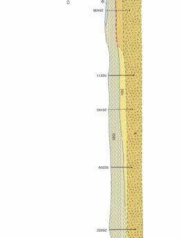
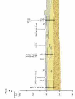
92 71 Figure 4.3. Cross-sections showing the surficial geology in the study area (Grimley et al., 2007; Phillips et al., 2001).

93 72 Flood plain deposits (alluvium) are bounded by the upland deposits (Peoria and Roxana Formation) both on the eastern and western margin of the quadrangles (see Figure 4.2 and Figure 4.3). Roxana Formation is the older of the two and is distinctively pinkish brown in color, has slightly more sand, coarse silt, and clay compared to the yellow brown Peoria Formation (Grimley and Lepley, 2005). These loess deposits are underlain by highly variable glacial till (Glasford Till) containing mixtures of sand, gravel, silt, and clay and usually unsorted in particle size. Glasford Till is highly variable in composition and texture from fat to lean clay to gravel. It also includes many discontinues sand and gravel lenses that can be tens of meters wide and up to 5 meters thick. In the Granite City quadrangle till may extend to bedrock at depths of meters. This is the usual case, however in the southeastern corner of the Monks Mound quadrangle till is underlain by Petersburg Silt and Banner Formation. Petersburg silt is the lake sediment, probably with loessial component and composed of mainly silt and silty materials up to 4 meters thick. Banner Formation is an older till deposition (pre- Illinois Episode) that contains relatively few sandy and gravely materials. Compared to the Glasford till, the Banner till is more clayey, slightly less stiff and has higher moisture content (Grimley and Lepley, 2005). Table 4.1. The lithologic units, classification and their ages (Grimley et al., 2001; Grimley and Lepley, 2005; Smith and Smith, 1984). Group Geologic Unit USC Classification Geologic age (C 14 years B.P) Lowland Cahokia Clay CH, CL, MH, ML Holocene (< 2,400) Cahokia Sand SP to CH, ML Holocene (8,500 2,400) Henry Formation SP, GP, GW Pleistocene (12,000 10,000) Upland Peoria and Roxana SP, CL Pleistocene (55,000-12,000) Formation Glacial Till SP, GP, CH, ML Pleistocene (190, ,000)

94 73 In the study area Cahokia clay, Cahokia sand, Cahokia fan, Henry Formation, Equality formation, undifferentiated alluvium, and disturbed ground are treated as Flood plain (or alluvial) group. Peoria silt, Roxana silt, Glasford till, Petersburg silt, and Banner till are all treated as Upland (or loess) deposits. A general stratigraphic column of the geologic units is given in Figure 4.4. As mentioned in the previous paragraphs, the seismic hazard analyses are based mainly on the accurate assessments of site amplifications that incorporate considerations of the underlying geologic conditions. For this purpose a soil cap thickness map was prepared for the surficial geologic units at the site which was used as input data in site amplification calculations INTERPOLATION TECHNIQUES AND THEORY Interpolation techniques are categorized as deterministic and geostatistic. Deterministic techniques use mathematical functions for interpolation; on the other hand geostatistic techniques apply both mathematical and statistical functions for interpolation. In other words; deterministic techniques create predicted surfaces from measured points where geostatistic techniques create not only predicted surface but also error or uncertainty of predictions map (Dunlap and Spinazola, 1984). Deterministic techniques are also divided into two groups: global and local. Global techniques calculate predictions from the measured points using the entire given dataset. Local techniques calculate predictions within the selected neighbor measurements where the closest measured dataset will have the highest influence. This is one rule of a thumb assumption where things that are closer together tend to be more alike than things that are farther apart. Inverse Distance Weighted (IDW), local polynomial and radial basis functions are known deterministic local interpolator techniques.

95 74 Figure 4.4. The stratigraphic column of the geologic units in the study area Geostatictical techniques are known as the Kriging techniques. The theory of kriging was first introduced by D. R. Krige for evaluating ore deposits and developed by Matheron (1971). Many methods are associated with this technique such as: simple kriging, ordinary kriging, universal kriging, probability kriging, indicator kriging, disjunctive kriging and cokriging. In these methods, kriging forms weights from surrounding measured values to predict values at unmeasured locations. It uses a linear estimation procedure to estimate a value at unsampled locations. The weights are based

96 75 on distance between the measured points and prediction location and on the overall spatial arrangement among the measured points: n X ( u ) = λ X ( u ) Eq. 4.1 o i= 1 i i Where X (u o ) is the estimated value at the unsampled location, X (u i ) is the value at the neighboring location u i and λ is the weight assigned to the neighboring value. Based on this equation, the unsampled location is estimated by a weighted average of the neighboring values. Kriging performs the calculations in two steps: in the first step it quantifies the spatial structure of the data and in the second step it produces a prediction based on the first step. Therefore, the most important step in kriging is the first step and this application of kriging is known as semivariogram, which allows examining the spatial autocorrelation between the measured sample points in spatial autocorrelation. To make a prediction at an unknown location, kriging will use this fitted semivariogram. The method of fitting to semivariogram differentiates the methods of kriging. Ordinary kriging is the most general and used of the kriging methods. This study used the ordinary kriging method to estimate and interpolate the geologic information; therefore, only ordinary kriging method will be summarized. The procedure and complex equations of ordinary kriging is given in various books (Isaaks and Srivastava, 1989; Kelkar and Perez, 2002) and journal papers (Mueller et al., 2004; Dunlap and Spinazola, 1984); hence only the important parameters will be shown here. Ordinary Kriging starts with an assumption of a model based on an unknown constant mean µ, and for the data and random errors ε (s) with spatial dependence. Z( s) = μ + ε ( s) Eq The above mentioned values are gathered after the preliminary consideration of the dataset by; i) defining a search neighborhood, and ii) conducting a cross-validation exercise. The search neighborhood defines how the neighboring sample points shall be

97 76 used in estimating values at unsampled locations (Kelkar and Perez, 2002). This relates to two parameters: i) the size of the neighborhood where the size should be large enough to include sufficient points and at the same time should be small enough for the selected sample points to be within the local region. Otherwise, the unwanted data points will also affect the calculations; ii) the shape and orientation of the neighborhood with quadrant divisions, which can be circular or ellipsoidal. These are important factors, because the major direction of spatial continuity can be sampled by this way (Figure 4.5). Figure 4.5. The search neighborhood defined in the dataset in terms of size and shape. The neighborhood is given an orientation to account for the anisotropic conditions. After the decision on the neighborhood properties, the semivariogram is constructed. This relationship of autocorrelation is captured in a semivariogram. The semivariogram (given in Figure 4.6) is a plot of the average of the squared difference

98 77 between the attribute values of a pair of points, verses the separation distance between the points. The equation for finding each point on the semivariogram is, n 1 2 γ ( h) = ( Z( X i ) Z( X i + h)) Eq n i= 1 Where γ is the semivariogram value plotted on the dependent axis, h is the separation distance between a pair of points, Z(i) is the attribute value at location i, and n is the number of pairs with separation distance h. The equation states in mathematical terms is that spatial data is said to be auto correlated if it is more likely for two points separated by a small distance to be similar than two points separated by a great distance. Ordinary Kriging makes use of the best-fit-line in the semivariogram (the yellow line in figure 4) to predict attribute values at locations where the attribute has not been measured. The best fit line is used to estimate weighting factors for neighboring locations in the process of predicting an attribute at an unmeasured location. The equation for this line is the empirical relationship between separation distance and attribute difference. Once this prediction process has been conducted for the entire study region, the result is a predicted continuous surface of the attribute value. The Eq. 4.1 is the predictor and it is the primary equation. The prediction calculations are performed for several locations. The matrix formula for Ordinary Kriging is given as, Γ * λ = g Eq. 4.4 Where Γ represents semivariance (semivariogram information), g is the modelled semivariogram value (prediction), and λ is the weighting value. This equation must be arranged to solve for λ, so the equation becomes, 1 λ = Γ * g Eq. 4.5

99 78 Where Γ -1 is the inverse matrix. Kriging is a geostatistical method that gives an indication of how good the predictions are. When the values are estimated for the unknown locations, it is beneficial to know the confidence level. One technique that the kriging uses is known as cross validation. In this technique, one sample point at a time is removed from the sample data, and using the remaining sample points, the value of the variable at now unsampled location is estimated. The estimated value is then compared with the observed value. This procedure is repeated at all sampled locations to have an estimated value at every sampled location. This application can identify obvious glaring errors, including decisions about stationary, appropriateness of the semivariogram model and search neighborhood (Kelkar and Perez, 2002); however it doesn t guarantee the success of the model. Figure 4.6. The semivariogram constructed for the top-of-bedrock prediction surface map. The number of lags were 10 and size was , enough to capture the details in the analysis.

100 79 After the cross-validation is performed for each point, an observed and an estimated value will be given for every point sampled. The problems with the estimation process can be revealed by comparing the observed values to the estimated values. The plot of estimated values vs. the true values are given in Figure 4.7. In the ideal situation an approximate equal number of values should be under- and overestimated over the entire region. The information from the estimated and the true values are used to estimate the error which is estimated by, * e( u ) = x( u ) x ( u ) Eq. 4.6 i i i Where e(u i ) is the estimation error at location u i, x(u i ) is the true value and x * (u i ) is the estimated value. Figure 4.7. The plot showing the predicted versus the true values of the input data. The blue line is the expected line (1:1) where the points are expected to fall linearly on this line. The scatter of the data gives the error estimate. It is a property of kriging that tends to underpredict large values and overpredict small values.

101 80 Different configurations can be plotted to examine the cross-validation to check the validity of the selected model (see Figure 4.8). In ideal conditions the error should be centered around the zero line with equal spread for n samples, 1 n e( u r i ) 0 n 1 i= Eq. 4.7 In the standardized error plot, the measurement values are subtracted from the predicted values and then divided by the estimated kriging standard errors. As mentioned before, the cross-validation gives an estimate of error and therefore the validity of the selected model and the parameters. The above explained steps make more sense when the quantification of the data set is made. This is accomplished by calculating the mean prediction error, the mean standardized error, the root-mean-square and the root-mean-square-standardized of the predicted and the measured data set. A good kriging model should reveal the following: i) The mean prediction error should be near zero. ii) The mean standardized error should be near zero. iii) The smaller the root-mean-square (RMS) prediction error, the better. iv) The root-mean-square standardized error should be close to one if the prediction standard errors are valid. If the RMS standardized error is smaller than 1, then the selected model mostly overestimates the values and if it is larger than 1, then the selected model mostly underestimates the model. In the ideal conditions the RMS standardized error should be close one indicating that the selected model is good. (See Figure 4.9).

102 81 (a) (b) (c) Figure 4.8. Plots showing the error estimation and examination of the cross-validation to check the validity of the selected model: (a) Error (true estimated) vs. true value during cross-validation, (b) The plot of standardized error vs. measured values, and (c) The Q-Q plot.

103 82 Figure 4.9. The prediction error calculations and checking for the validity of the selected model MODELING SUBSURFACE INFORMATION One of the most important parameters in site-response analysis is the thickness of surficial materials capping the bedrock, because of impedance contrasts that often occur at this boundary. In regional studies it is often useful to begin the assessment process by constructing a detailed depth-to-bedrock map, which compares existing ground elevations with the elevations at the top of the buried bedrock basement. The ordinary kriging method can be employed to estimate and interpolate the depth-to-bedrock interface from disparate borehole data points, using software like ArcGIS version 9.1. The ordinary kriging method uses the information from adjacent data points to predict the elevation of any given horizon of interest by incorporating the autocorrelation structure of the adjacent data. The primary advantages of the kriging method are its ability to: 1) interpolate an actual value at measured data points, and 2) to provide kriged estimates and the corresponding uncertainties at all locations between the known data points. Subsurface information was gleaned from digitized well logs prepared by the Missouri and Illinois Departments of Transportation. Stratigraphic interpretations and geologic cross sections were prepared by the Missouri and Illinois geological surveys, based on information gleaned from field exposures, geophysical surveys, and well logs (geotechnical, water wells, mining, environmental). In order to fill some of the data gaps between the boreholes, interpretations of the bedrock surface made by the ISGS

104 83 were incorporated into the database. The locations of the borings and well logs are shown in Figure Since all three of the study quadrangles bounded the Wood River quadrangle, well data from this quadrangle was also compiled in the database, to reduce edge effects on the study quads. Figure Location of borings and well logs that were used in the study to estimate the lithologic variations beneath Granite City, Monks Mound and Columbia Bottom Quadrangles. Several techniques can be used to estimate the thickness of surficial units capping the bedrock basement. The first generation maps were created using standard kriging methods to create a surficial deposits isopach (thickness) map. This approach proved

105 84 untenable because the map was incapable of capturing fine details, such as the variations in thickness along stream valleys (where material had been eroded) and the boundary between the uplands and the floodplains could not be discerned! This necessitated that alternative methods be developed to incorporate considerations of topographic relief and pinching/interfingering of surficial units near their respective boundaries. This method was successfully applied in the coal resource assessment map for the Amoret Quadrangle, Missouri, which estimates the thickness of the Mulberry coal and the thickness of the overburden (Mulvany, 2007). Depth-to-bedrock values were determined by applying the following procedure: i) Top-of-bedrock elevation values were determined using the above mentioned sources and interpretations. Depths are referenced from the National Elevation Datum. See Figure 4.10 for the locations of these data sources. ii) Using these top-of-bedrock elevation values and ArcGIS Geostatistical Kriging Tool, a map showing the predicted surfaces was constructed using kriging techniques. This map was named the Top of Bedrock Elevation (TBRE). This map is shown in Figure iii) The 30 m digital elevation model (DEM) of USGS was imported into ArcGIS (Figure 4.13). iv) Using the Spatial Analyst Tool in ArcGIS, the top of bedrock elevation was digitally subtracted from the USGS DEM to ascertain the depth-to-bedrock from the existing ground surface (ignoring the uncertainty in the USGS DEM elevations). The resulting product was an isopach map that is mathematically conformable with the topographic surface and the top-of-bedrock surface. This area in between is referred to as surficial materials (soil cap) thickness maps, or depth-to-bedrock maps. This map is shown in Figure The isopach map of surficial materials was based on two surfaces rather than on scattered points (extracted from boring logs). The extent to which the isopach values are in error would emanate from uncertainties in the kriging method and in the reported bedrock elevations on the boring logs. The interpretations recorded on boring logs

106 85 usually involve some measure of judgment on the part of whoever is logging the boring/well, and whether cores were retrieved and examined, as opposed to cuttings RESULTS AND DISCUSSION The top-of-bedrock map shows the surface varies between a minimum value of 47 meters beneath the Mississippi River flood plain (in the Columbia Bottom quad, which may be an old sinkhole), to a maximum altitude of 163 meters in the elevated loess covered uplands. The bedrock surface changes most abruptly at the lateral margins of the modern day flood plain, which coincides with the boundary between loess and alluvium. The bedrock surface beneath the Mississippi River flood plain appears to be an even planated surface, with an elevation between 90 and 100 meters. As mentioned previously, ordinary kriging was employed in these estimates because it provides estimates or error using known parameters. An error estimate map was generated for the estimated top-of-bedrock elevations, shown in Figure According to the calculations, the error ranges from 1.8 meters to as much as 18.4 meters. The highest error distributions correspond to the areas where there is little or no subsurface (borehole) data (compare Figures 4.10 and 4.12). In the study area east of the Mississippi River the error estimates are in the order of 1.8 to 9 meters, smaller than on the west side of the river, because of the disparity in areal distribution of the subsurface data points, which tend to be clustered and widely separated west of the Mississippi River (there is scant development or infrastructure in much of the river s flood plain, below the confluence of the Mississippi and Missouri Rivers). Within the modern floodplains the alluvial thickness is fairly uniform, between 30 and 40 meters, thinning to as little as 5 meters at the lateral margins bounding the elevated uplands. At the boundary between the floodplain and uplands, there is often a sudden increase in thickness caused by accumulation of small fans from watercourses draining the elevated uplands. The thickness of the soil cap in the loess covered uplands varies considerably (between 5 and 73 meters) because the loess reaches its maximum thickness at the lateral margins of the Mississippi River flood plain (along the bluffs), although it exhibits a more uniform thickness in the Monks Mound quadrangle. In the Columbia Bottom area the soil cap thickens markedly beneath the highest portions of the

107 86 elevated uplands because these have not been dissected and eroded as much (due to insufficient tributary watershed). In the Granite City quadrangle the thickness seems to be more uniform, varying between 5 to 20 meters. At the very south end of the Granite City quadrangle, however, the thickness varies locally along old channels and sinkhole features (confirmed by borings in the downtown area). Bedrock (thickness of zero) is only exposed in the northwest portion of the Columbia Bottom Quadrangle in the bluffs bordering the south side of the lower Missouri River. These results are based on the available boreholes and on the assumptions inherent in the kriging method used to estimate top-of-bedrock elevations. In the map, karstic features were not taken into account because of the limited density of available boreholes, but sinkholes are recognized to pervade much of the study area, and are likely responsible for one highly anomalous feature in the northwest quarter of the Columbia Bottom quadrangle, along the southern side of the Missouri River flood plain (where a thickness of almost 80 m is shown on the depth-to-bedrock map).

108 Figure Top-of-bedrock elevation map as estimated using the ordinary kriging method 87

109 Figure Prediction standard error map of top-of-bedrock elevation map as estimated using the ordinary kriging method. 88

110 Figure Digital Elevation Model from United States Geological Survey 89

111 90 Figure Estimated depths to top of bedrock (or surficial materials thickness). Several general characteristics were resolved by modeling these lithologic boundaries. The greatest uncertainty exists where the model was based on data extrapolated from distant sources and where the observations were increasingly sparse. The principal advantages of kriging are summarized below: i) Other methods (deterministic methods) have no assessment of prediction error.

112 91 ii) Kriging methods assess the error of prediction assuming normallydistributed data iii) Prediction maps (interpolated maps) provide estimates in the areas without observations or measurements, between established data points. iv) Standard error maps (the square root of the variance of a prediction) present a spatial distribution of prediction error for an estimated surface. The predicted error increases with increasing distance from adjacent data points. The relation between the DEM, TBRE and standardized errors can be appreciated by constructing and examining the cross-sections (S1, S2, S3, S4, S5, S6, and S7), presented in Figures l8. The locations of these cross-sections are shown in Figure Seven cross-sections were constructed to illustrate the estimated position of the top of bedrock along with the standardized error. In cross-sections S4 and S7 the top-ofbedrock surface appears nearly horizontal and parallel to the flood plain surface. The bedrock surface tends to gain elevation approaching the elevated uplands bounding the flood plain. Cross sections S1 and S2 show the steep gradient of the bedrock surface approaching the lateral margins of the modern flood plain. The bedrock interface (blue line) is steeply incised at the lateral margins of the flood plain, and the soil cap tends to pinch out. In the elevated uplands bounding the flood plain the bedrock surface is not so severely planated, and exhibits considerably more undulation at the higher elevations. The thick blanket of loess overlying the elevated uplands is locally incised by recent (Holocene) erosion, exhibiting a much more uneven surface. The ISGS cross-sections and the predicted top-of-bedrock profiles exhibit similar forms, in agreement with the boring logs. Even though kriging is a practical geostatistical tool that provides interpolated surfaces with a corresponding estimate of error, it also makes predictions of standard error that are occasionally unrealistic, showing the upper bound error above the ground surface (see Figures 4.16 an 4.17). This unrealistic portrayal highlights some of the problems inherent with estimates of error, which will always require some judgment to assess their actual or perceived significance. Obviously, the more dense the pattern of borings (data), the more reliable the predictions and the smaller the calculated errors.

113 92 When the bedrock surface is more or less uniform there is little uncertainty in the calculations. However, sloping contacts (like those shown in Figures 4.16 thru 4.18) will always complicate the predictions, especially when the slope becomes increasingly severe. In order to minimize the problems associated with this effect, additional (interpreted) data points were inserted to define topographic anomalies, such as the steeply incised loess covered uplands (shown in Figures 4.16 thru 4.18). The addition of these artificial data points produces a more reliable top-of-bedrock surface map because the complex boundary conditions are better represented. Kriging can also be problematic in the loess covered uplands. The loess deposits mantling uplands tend to thicken towards hilltops and thin in the valley bottoms because of erosion. Statistically, very few borings exist within these valley bottoms, so the loess thickness values are biased towards the thicker sections mantling the adjacent uplands. This disparity causes kriging techniques to be somewhat unreliable, as shown in Figure Kriging (as well as all other prediction methods) assumes that different data sets will represent different areas that are spatially unique. For these reasons, artificial data points were inserted along the deep valleys to minimize the predicted errors.

114 Figure Locations of profiles that were utilized to compare the estimated topography and the predicted top-to-bedrock, with the standardized error. Cross-section C-C was used for quality control of the underlying stratigraphy and draw comparisons between the interpreted and predicted surfaces. 93

115 Figure Cross-sections showing the variations in the topographic surface, top-ofbedrock, and the associated uncertainties for S1 and S2 (see Figure 4.15 for the locations of the profiles). 94

116 Figure Cross-sections showing the variations in the topographic surface, top-ofbedrock, and the associated uncertainties for S3 and S4 (see Figure 4.15 for the locations of the profiles). 95

117 Figure Cross-sections showing the variations in the topographic surface, top-ofbedrock, and the associated uncertainties for S5, S6 and S7 (see Figure 4.15 for the locations of the profiles). 96

118 97 The depth-to-bedrock map provides useful information about regional variations in the thickness of the surficial (unconsolidated) geologic units recognized in the St. Louis area. The estimated uncertainties of these predicted surfaces using Kriging provided a range of possible values (minimum and maximum). These variations in thickness and their associated uncertainties were input into site amplification estimations. The various uncertainties and errors associated with kriging (summarized above) create some intrinsic problems with estimating site amplification factors, which should always be appreciated. In addition, the larger valleys developed in the uplands are mapped as alluvium, and are assumed to be underlain by Paleozoic bedrock. However, a few of the boring logs show that the recent alluvium is underlain by loess deposits. The site response calculations did not take this local effect into account. Figure The loess deposits mantling the elevated uplands tend to thin towards the valleys, due to recent erosion. Very few borings are situated in the valleys. When thickness data is missing in these valleys, kriging techniques can be unreliable, as shown by the dotted red line.

119 98 5. VARIATIONS IN SHEAR-WAVE VELOCITY 5.1. INTRODUCTION Shear-wave velocity is commonly used in practice to classify the soil deposits for seismic site response. One way is to classify the soil-type shear-wave velocity for the upper 30 meters. Recent National Earthquake Hazards Reduction Program (NEHRP) classifies these into five main categories that were given in Table 2.2. The NEHRP classification of a site is based primarily on a time-averaged shear-wave velocity to a depth of 30 m (V S 30) as shown in Equation 2.2, Section 2. This method of classification is one of the most preferred, because of its use in the recent building code provisions (BSSC, 2001; 2003). Velocity profiles may be measured directly or inferred from correlations of shear wave velocity with penetration resistance or undrained shear strength. For the seismic design of a code-compliant structure, the Vs 30 beneath the structure determines the appropriate short- and mid-period amplification factors to be applied to modify the reference earthquake spectra (e.g., Dobry et al. 2000). This classification also considers site amplification when estimating the seismic demand on a structure. For this reason two amplitude-dependent site amplification factors are specified: F a for short periods and F v for longer periods (Dobry et al., 2000; Choi and Stewart, 2005). These NEHRP site factors are based on both empirical data analysis and results of ground response analyses (Dobry et al., 2000). A number of studies have investigated the validity of these factors (such as Borcherdt, 2002a, b; Harmsen, 1997; Field, 2000; and Choi and Stewart, 2005), some suggesting significant discrepancies between their results and the factors given in the building code provisions. Other classification systems that incorporate site specific parameters are proposed as well. For example, Rodriquez-Marek et al. (2001) classified the sites based on two primary parameters (type of deposit and depth to bedrock) and two secondary parameters (depositional age and soil type). The authors stated that they provided the additional subdivision in order to capture the anticipated different nonlinear responses of the soils while allowing the evaluation of the importance of soil depth on seismic site response.

120 99 Wills et al. (2000) found the geologic units to provide useful proxies for estimating shear-wave velocity characteristics needed for seismic hazard calculations. Shear-wave velocity is found to be an appropriate measure of rock or soil conditions for ground motion calculation because it directly affects ground motion amplification due to differences associated with material properties (Wills and Silva, 1998). Shear-wave velocity was also determined to be very effective in classifying the geologic units for calculating the intensity of shaking because it is dependent on physical properties of the material such as porosity, density, cementation, hardness, competence, and joint intensity of rock. However, classifying the soils based on only shear-wave velocity values may not be appropriate in all cases. For example, the shear wave velocity classification scheme does not consider the depth of the soil profiles and the weathering characteristics of the base rock. It has high standard errors which introduces undesirable levels of uncertainties in ground motion prediction (Rodriquez-Marek et al. 2001). Choi and Stewart (2005) also noted that detailed surface geology based classification schemes are more effective than NEHRP categories. To avoid these problems, a site-specific earthquake analysis should be employed. This method generally found to provide good estimates of the site response especially when the local site geology and their engineering properties are known. In this study, the shaking level at the top of the soil profile is characterized using the site-specific earthquake analysis, then employing the probabilistic and deterministic hazard analysis approaches. The shaking level calculations primarily based on the siteamplification calculations which largely depend on the predicted shear-wave velocities of the materials present at the site. In fact in numerous studies shear-wave is found to be the material property that influences the ground motions most strongly (Field, et al., 2000, Wills et al., 2000, Holzer, et al., 2005a). In addition, several investigations (Gomberg et al., 2003; Romero and Rix, 2001, Field, et al., 2000, Wills et al., 2000) have suggested that the shear-wave velocities depend strongly on the lithology; therefore meaningful characteristic shear wave velocity profiles (CSVP) only can be generated for a reference depth-to-bedrock map which was explained in the previous section.

121 100 In this section, the methodology on the characterization of the regional shearwave velocities was summarized. The methodology explained herein resembles of that explained in Romero and Rix (2001, 2005) and Gomberg et al. (2003). The regional shear-wave velocities were determined for two distinct lithologic units; alluvium and loess. Local analyses were performed to ascertain variations, uncertainties, and randomness associated with the shear-wave velocity profiles. These data then were grouped based on the age and stratigraphy. This approach included three locations capped by alluvial deposits and six locations capped by wind-blown deposits. The uncertainties in dynamic geophysical properties were then incorporated into a series of regional shearwave velocity profiles (SWVP) to better approximate the characteristic profile of the Quaternary age cover lying atop the Paleozoic age basement. The characteristic SWVPs were compiled after correlating this information with the lithologic structure (depth-tobedrock) recognized beneath the St Louis area. This study used 76 site-specific shearwave velocity profiles to compile characteristic SWVPs needed to calculate seismic site amplification across the entire St. Louis Metro area over the next decade. In summary, characteristic profiles were determined following a 4 step procedure. The first step was already explained in Section 4. The latter steps are explained in more detail in the subsequent sections. i. Investigation of geology from the available borehole logs and estimations of the stratigraphy underlying each point of calculation; ii. Determination of mean Vs with uncertainties from local Vs profiles (groups), in one meter depth increments; iii. Comparing the variations in Vs values with borings and known limiting parameters, such as depth-to-bedrock; iv. Application of the statistical rules to determine the average values with the estimated geologic boundaries COMPILATION OF SHEAR WAVE VELOCITY PROFILES Shear wave velocity profiles were compiled for the St Louis Area from various sources. Table 5.1 lists each site, the source of profile, type of test performed, estimated Vs for 30 meters, corresponding NEHRP site class, and description of the surficial

122 101 material upon which the tests were performed. The velocity profiles were measured using various methods, such as reflection and refraction, multi-spectral analysis of surface waves (MASW), seismic downhole tests, and seismic cone penetrometer test (SCPT) methods. The University of Missouri-Rolla developed Vs profiles based on MASW interpretive techniques. The test sites were located in the following quadrangles in proximity to the study area: Granite City, Monks Mound, Columbia Bottom, Cahokia, and Clayton. 25 profiles were developed in flood plain alluvial sites and 31 profiles were developed in loess covered uplands. The Illinois State Geological Survey prepared five Vs profiles using the seismic downhole method. All of these Vs profiles were developed for the flood plain deposits. The United States Geological Survey prepared 15 profiles using the Reflection/Refraction method; eight in the mapped flood plain and seven in loess covered uplands. Eight profiles were developed by private consultants for the Missouri Department of Transportation using the SCPT method. These profiles do not extend deeper than 7 meters and they were performed on loess covered upland sites in the Cahokia Quadrangle. Five additional profiles were developed by private consultants in the St. Louis area. Three of these profiles were measured by Hanson Engineers, Inc. for the new Interstate 70 Bridge over the Mississippi River; and two profiles were prepared by Geotechnology, Inc. for the Grand Avenue Bridge rehabilitation project. The locations of the compiled shear wave velocity profiles within the St. Louis Metro area, Missouri and Illinois, are presented in Figure 5.2.

123 102 Table 5.1. Compiled shear-wave velocity measurements collected in the St Louis Metropolitan Area, Missouri and Illinois ID Source Method Quadrangle Surficial Material V s m/sec UMR-12 UMR MASW Granite City Alluvium 235 D UMR-13 UMR MASW Granite City Alluvium 239 D UMR-55 UMR MASW Granite City Alluvium 231 D UMR-56 UMR MASW Granite City Alluvium 255 D UMR-57 UMR MASW Granite City Alluvium 209 D UMR-58 UMR MASW Granite City Alluvium 275 D UMR-59 UMR MASW Granite City Alluvium 233 D UMR-60 UMR MASW Granite City Alluvium 234 D UMR-61 UMR MASW Granite City Alluvium 262 D UMR-83 UMR MASW Granite City Alluvium 236 D UMR-46 UMR MASW Monks Mound Alluvium 254 D UMR-47 UMR MASW Monks Mound Alluvium 194 D UMR-48 UMR MASW Monks Mound Alluvium 213 D UMR-49 UMR MASW Monks Mound Alluvium 197 D UMR-50 UMR MASW Monks Mound Alluvium 199 D UMR-51 UMR MASW Monks Mound Alluvium 224 D UMR-52 UMR MASW Monks Mound Alluvium 200 D UMR-53 UMR MASW Monks Mound Alluvium 159 D UMR-54 UMR MASW Monks Mound Alluvium 219 D UMR-74 UMR MASW Monks Mound Alluvium 232 D UMR-67 UMR MASW Columbia Bottom Alluvium 347 D UMR-68 UMR MASW Columbia Bottom Alluvium 221 D UMR-69 UMR MASW Columbia Bottom Alluvium 209 D UMR-70 UMR MASW Columbia Bottom Alluvium 192 D UMR-71 UMR MASW Columbia Bottom Alluvium 259 D UMR-72 UMR MASW Columbia Bottom Alluvium 254 D UMR-73 UMR MASW Columbia Bottom Alluvium 228 D UMR-14 UMR MASW Cahokia Alluvium 396 D UMR-75 UMR MASW Cahokia Alluvium 246 D UMR-76 UMR MASW Cahokia Alluvium 232 D UMR-78 UMR MASW Cahokia Alluvium 137 D UMR-79 UMR MASW Cahokia Alluvium 221 D UMR-80 UMR MASW Cahokia Alluvium 243 D UMR-84 UMR MASW Cahokia Alluvium 221 D UMR-21 UMR MASW Webster Groves Alluvium 240 D HSL4 ISGS Downhole Monks Mound Alluvium 232 D HSL2 ISGS Downhole Monks Mound Alluvium 267 D 3L ISGS Downhole Monks Mound Alluvium 220 D UMR-2 UMR MASW Granite City Loess 615 C UMR-3 UMR MASW Granite City Loess 350 D UMR-4 UMR MASW Granite City Loess 278 D UMR-6 UMR MASW Granite City Loess 327 D (30m) NEHRP Soil Class

124 103 ID Source Method Quadrangle Surficial Material V s m/sec UMR-7 UMR MASW Granite City Loess 249 D UMR-8 UMR MASW Granite City Loess 258 D UMR-9 UMR MASW Granite City Loess 302 D UMR-10 UMR MASW Granite City Loess 295 D UMR-11 UMR MASW Granite City Loess 182 D UMR-43 UMR MASW Granite City Loess 306 D UMR-44 UMR MASW Monks Mound Loess 249 D UMR-45 UMR MASW Monks Mound Loess 201 D UMR-62 UMR MASW Columbia Bottom Loess 275 D UMR-63 UMR MASW Columbia Bottom Loess 307 D UMR-64 UMR MASW Columbia Bottom Loess 259 D UMR-65 UMR MASW Columbia Bottom Loess 244 D UMR-66 UMR MASW Columbia Bottom Loess 298 D UMR-1 UMR MASW Cahokia Loess 295 D UMR-15 UMR MASW Cahokia Loess 506 C UMR-16 UMR MASW Cahokia Loess n/a n/a UMR-77 UMR MASW Cahokia Lacustrine 271 D UMR-81 UMR MASW Cahokia Loess 386 C UMR-5 UMR MASW Clayton Loess 416 C UMR-29 UMR MASW Clayton Loess 419 C UMR-30 UMR MASW Clayton Loess 293 D UMR-31 UMR MASW Clayton Loess 363 D UMR-32 UMR MASW Clayton Loess 406 C UMR-34 UMR MASW Clayton Lacustrine 321 D UMR-35 UMR MASW Clayton Loess 346 D UMR-37 UMR MASW Clayton Loess 470 C UMR-38 UMR MASW Clayton Loess 335 D UMR-39 UMR MASW Clayton Loess 368 C UMR-40 UMR MASW Clayton Loess 315 D UMR-41 UMR MASW Clayton Loess 285 D T4-3 MoDNR SCPT Clayton Loess n/a n/a T41-1 MoDNR SCPT Clayton Loess n/a n/a T29-1 MoDNR SCPT Clayton Loess n/a n/a T26-1 MoDNR SCPT Clayton Loess n/a n/a T143-1 MoDNR SCPT Clayton Loess n/a n/a T14-2 MoDNR SCPT Clayton Loess n/a n/a T133-2 MoDNR SCPT Clayton Loess n/a n/a T132-1 MoDNR SCPT Clayton Loess n/a n/a 64-9 MoDNR SCPT Clayton Loess n/a n/a 64-8 MoDNR SCPT Clayton Loess n/a n/a 64-7 MoDNR SCPT Clayton Loess n/a n/a 64-4 MoDNR SCPT Clayton Loess n/a n/a 64-2 MoDNR SCPT Clayton Loess n/a n/a MoDNR SCPT Clayton Loess n/a n/a ARMO USGS Reflection/ Refraction (30m) Oakville Alluvium 200 D NEHRP Soil Class

125 104 ID Source Method Quadrangle Surficial Material SCSF USGS Reflection/ Refraction HLSP USGS Reflection/ Refraction THIES USGS Reflection/ Refraction CHES USGS Reflection/ Refraction CHS USGS Reflection/ Refraction EC USGS Reflection/ Refraction FENTON USGS Reflection/ Refraction 8THCAS USGS Reflection/ Refraction STLU USGS Reflection/ Refraction HPSL USGS Reflection/ Refraction 22NDMA USGS Reflection/ D Refraction HES USGS Reflection/ Refraction FLWALL USGS Reflection/ Refraction MVU USGS Reflection/ Refraction SCOT USGS Reflection/ Refraction SCCC USGS Reflection/ Refraction V s m/sec (30m) Grafton Alluvium 200 D Monks Mound Alluvium 210 D Creve Coeur Alluvium 225 D Weldon Spring Alluvium 235 D Monks Mound Loess 245 D St Charles Alluvium 250 D Kirkwood Alluvium 290 D Granite City Loess 410 C Granite City Loess 430 C Granite City Loess 460 C Granite City Loess 560 C Wentzville Loess 595 C Granite City Loess 620 C Creve Coeur Loess 720 C St Charles Loess 740 C O'Fallon Loess 785 B NEHRP Soil Class The shear wave velocity profiles were analyzed, based on local geographic and lithologic characteristics, and then recompiled to develop regional generic profiles. These local sites were chosen based the age of the respective surficial geologic units and on their geographic location. Three local analyses were performed for alluvial filled flood plains and six local analyses were performed for loess covered uplands, which are summarized in Table 5.1.

126 UNCERTAINTIES IN SHEAR-WAVE VELOCITY Statistically, there are usually two uncertainties associated with the determination of insitu shear-wave velocities. The epistemic uncertainty is the ability to accurately predict a given parameter based on the available measured data, due to such factors as: limited data, data interpretation, and testing procedures (Toro et al., 1997; Romero and Rix, 2001). The epistemic uncertainty can be reduced by the acquisition of additional data, or by improving data acquisition and interpretation techniques. The aleatory uncertainty is due to the inherent heterogeneity of naturally deposited geologic materials and may not be reduced by the collection of additional or higher quality subsurface data (Toro et al., 1997; Romero and Rix, 2001). Nine areas were delineated for construction of representative shear wave velocity profiles. Vs data collected in each of these areas was grouped together for assessment of the various uncertainties associated with measured Vs values and the uncertainties associated with the depth, thickness, and consistency of the recognized surficial geologic units. These groupings sought to generalize the local characteristics of specific geomorphic provinces surrounding St. Louis, combining all of the data collected in sitespecific profiles. Three of these areas were within the modern flood plains and six were selected to represent the loess covered uplands (see Figure 5.1). For each area, the geometric mean of the shear wave velocity at 1-meter depth increments were calculated. After comparing these 1-meter increment mean Vs profiles with the nearest boring logs, the characteristic profiles were crafted for each of the areas shown in Figure 5.1. The characteristic profiles were constructed by considering the following criteria: i) determination of the mean Vs from local Vs profiles for each 1 meter depth increment; ii) ascertain local variations in depth, thickness, and consistency of the surficial geologic units from borehole logs; and, iii) determination of the characteristic profiles after comparing the variations in Vs and the underlying stratigraphy.

127 106 Figure 5.1. Areal distribution of the nine areas delineated for construction of representative shear wave velocity profiles. These were designated as: Pleistocene Granite City (P-GC), Pleistocene Columbia Bottom (P-CB), Pleistocene Clayton (P-CL), Pleistocene Clayton DNR (P-DNR), Pleistocene Webster (P-WB), and, Pleistocene Monks Mound (P-MM). The uncertainty analyses performed for shear wave velocities assumed that the differences in test techniques and the differences in data measured by these techniques are somewhat negligible. However, the comparisons between these tests indicated that the difference between them can be up to 30% (Bauer, 2007). Some of the disagreements in the measured Vs values can also be attributed to the stratigraphic variations in the soil where the measurements were performed. Since it was difficult to distinguish the variability in stratigraphy, the data points selected for the areal shear wave velocity analyses were assumed that they were measured at similar conditions.

128 Flood Plain Deposits. Three areas felt to be representative of the alluvial filled flood plains were delineated as shown on Figure 5.1. Area H-CC is situated within the Monks Mound quadrangle and is dominated by deposits of Holocene age Cahokia clay. The second area was designated as H-CS, and it straddles the boundary between the Granite City and Monks Mound quadrangles. Near the ground surface the H-CS area is underlain by Holocene age Cahokia sand. The H-CB area covers the modern flood plain near the confluence of the Mississippi and Missouri Rivers, on the Columbia Bottom Quadrangle. In this area the flood plain is underlain by Cahokia clay, Cahokia sand, and the older Henry Formation (Pleistocene sand/gravel deposits). Table 5.2. Areas selected for representative Vs profiles. See Figure 5.1 for locations. Age and Unit Area Name Area Designation Topography Holocene Age Cahokia Clay H-CC Flood plain Alluvium Group Cahokia Sand H-CS Flood plain Columbia Bottom H-CB Flood plain Pleistocene Age Loess Group Columbia Bottom P-CB Upland Clayton P-CL Upland Granite City P-GC Upland Webster Grove P-WG Upland Monks Mound P-MM Upland Clayton DNR P-DNR Upland Thirteen profiles were compiled in area H-CC, eleven which were measured by MASW techniques, one seismic downhole test series, and another that employed the reflection/refraction method. Eight profiles were grouped together for area H-CS, six of which were measured by employing MASW and two seismic downhole tests. Six profiles were compiled in area H-CB, all from MASW tests. In all these local Vs analyses, Vs

129 108 was assumed to be a normally distributed random variable at each depth increment. In all of these areal groupings, depth versus Vs, standard deviation, and coefficient of variance plots were calculated and plotted. These plots are presented in Figures 5.2 thru 5.4. The data exhibited a steady increase in the reported shear-wave velocities with depth, irrespective of material type or geologic age. Standard deviation and coefficient of variance also appeared to increase with depth, because of increasing scatter of Vs measurements. A curious aspect was the high standard deviations and increased coefficient of variance noted in the upper few meters of the measured Vs profiles. The high degree of variability in the upper 1 to 2 meters may be ascribable to man-caused disturbance, engendered by surficial grading, filling, and structural surcharging (by transient traffic loads or by structures and/or stockpiling). The mean coefficient of variation (the ratio of standard deviation to the mean) range from about 15.5 % to 17.6 % for the Cahokia Formation, and 13.3 % to 20.8 % for the older Henry Formation (see Table 5.3). These low mean coefficients of variance (< 25%) suggest that there is an acceptable variation of Vs for the calculated mean Vs. Figure 5.5 presents three plots comparing the average of shear wave velocity with depth in the Cahokia and Henry Formations that typify the alluvial fill in the Mississippi flood plain. These illustrate the groups for flood plain areas H-CC, H-CS, and H-CB. The estimated positions of the formational contacts were deduced from adjacent boreholes.

130 109 (a) (b) (c) Figure 5.2. Plots of (a) Mean velocity, (b) Standard deviation (σ), and (c) coefficient of variation (COV) profiles with depth for H-CC. (a) (b) (c) Figure 5.3. Plots of (a) Mean velocity, (b) Standard deviation (σ), and (c) coefficient of variation (COV) profiles with depth for H-CS.

131 110 (a) (b) (c) Figure 5.4. Plots of (a) Mean velocity, (b) Standard deviation (σ), and (c) coefficient of variation (COV) profiles with depth for H-CB. (a) (b) (c) Figure 5.5. Comparison of generated local Vs profiles in Holocene age deposits; a) H- CC, b) H-CS and c) H-CB. Shown on the graph are the characteristic profile (CH-PRO), estimated uncertainty upper bound (EU-UB) and estimated uncertainty lower bound (EU- LB). Top 5 meters is characterized by Cahokia clay in H-CC and H-CB profiles which is missing in H-CS profile. Cahokia sand is found at ~17 meters in all profiles.

132 111 Table 5.3. Statistics of Vs distributions mean, standard deviation (SD) and coefficient of variance (COV)- of Floodplain alluvium deposits. Cahokia Formation Henry Formation Average Vs (m/s) SD (m/s) COV (%) Average Vs (m/s) SD (m/s) COV (%) H-CC H-CS H-CB Loess Covered Upland Deposits. Six areas felt to be representative of the loess covered uplands were delineated, as shown on Figure 10. Five of these were located on the Missouri side of the Mississippi River (Granite City loess, P-GC; Columbia loess, P-CB; Clayton loess, P-CL; Clayton loess DNR, P-CLD; Webster loess, P-WB), and one area is located on the Illinois side of the Mississippi River (Monk loess, P-MM). The thickness of the loess varies between zero and 75 m on the Missouri side and 5 m to 45 m on the Illinois side of the Mississippi River. These reference profiles were more difficult to construct because of areal scatter and separation of the boreholes and local variations in loess thickness (shown in Figure 4.19). The area profiles containing the measured data in the loess covered uplands are shown in Figure 5.6. Each profile was interpreted by comparing it to the nearest borehole. Due to the much wider range in thickness of the loess cover, the depth of the Vs measurements vary considerably, from ~7 to ~20 m. The uncertainty analyses, standard deviations, and coefficient of variation of each profile tend to increase with depth, similar to the profiles generated in the alluvial flood plain. The P-MM profile exhibits more uncertainty than the other upland profiles because it only contains data from three measurement sites (the only existing Vs data in the uplands on the Monks Mound Quadrangle).

133 112 (a) (b) (c) (d) (e) (f) Figure 5.6. Comparison of average local Vs profiles in loess covered uplands; a) Pleistocene Granite City (P-GC), b) Pleistocene Columbia Bottom (P-CB), c) Pleistocene Clayton (P-CL), d) Pleistocene Clayton DNR (P-CHD), e) Pleistocene Webster (P-WB), and f) Pleistocene Monks Mound (P-MM).

134 113 (a) (b) (c) (d) (e) Figure 5.7. Plots illustrating the standard deviation and coefficient of variation with depth for local Vs profiles in the loess covered uplands; a) Pleistocene Granite City (P-GC), b) Pleistocene Columbia Bottom (P-CB), c) Pleistocene Clayton (P-CL), d) Pleistocene Clayton DNR (P-CHD), and e) Pleistocene Webster (P-WB).

135 CHARACTERISTIC SHEAR-WAVE VELOCITY PROFILES (CSVP) The procedure to estimate the contact depth of mapped stratigraphic units (e.g. Cahokia Clay, Cahokia sand, Henry Formation) was described above. Representative velocities for each mapped unit were then assigned and compared to the local shear-wave velocity analyses before crafting the characteristic shear wave velocity profiles. Previous compilers of characteristic Vs profiles have proposed that the distribution of Vs within recognized geologic units is usually lognormal (EPRI, 1993; Romero and Rix, 2005). The variability of Vs within recognized stratigraphic units suggest that the St. Louis data is best represented by assumed log-normal distributions. This finding was confirmed by chi-square tests for goodness-of-fit (Ang and Tang, 2007). In the chi-square test, the similarity between the assumed distribution and the data set is evaluated using the equation: k i= 1 2 ( n e ) 2 i e χ = Eq. 5.1 e i Where n i is the observed frequencies, e i is the expected frequencies, and k is the number of data intervals. Ang and Tang (2007) pointed out that it is generally necessary to have k>5 and e i >5 in the chi-square test for goodness-of-fit. The difference between the lognormal and normal distributions also decreases with variance (Ang and Tang, 2007). When the coefficient of variation is less than 25%, normal and lognormal distributions are difficult to distinguish (Holzer et al., 2005b). It can be appreciated from Table 5.3 that the calculated coefficient of variation values are consistently less than 25%. This could explain why the estimated Vs values are so similar.

136 115 Table 5.4. Computation of chi-square test for normal and lognormal distribution assumptions for Cahokia (top table) and Henry (bottom table) Formations. Interval Observed Expected Frequencies (e i ) Chi-square (χ 2 ) m/sec Frequency, n i Normal Lognormal Normal Lognormal < > χ 2 = Interval Observed Expected Frequencies (e i ) Chi-square (χ 2 ) m/sec Frequency, n i Normal Lognormal Normal Lognormal < > χ 2 = The chi-square χ 2 was determined for 5 meter depth increments as well as for all of the data sets. The chi-square calculations for Cahokia Formation, Henry Formation, alluvium, and loess are tabulated in Tables 5.4 and 5.5, respectively. Statistical

137 116 calculations, in terms of chi-square test, mean Vs values, and standard deviations are shown in Table 5.6. It can be appreciated from Tables 5.3 thru 5.6 that it would appear that lognormal distributions represent the Vs data better than the normal distributions. This is apparent from the lower chi-square values. The probability density functions and histograms of Vs for the recognized stratigraphic units are plotted and compared in Figures 5.10 thru The median and average values of Cahokia, Henry, alluvium and loess were determined to be: 171 m/sec, 275 m/sec and 208 m/sec, and 174 m/sec, 288 m/sec, and 231 m/sec respectively. The combined alluvium unit shear wave velocity was calculated to be 200 m/sec (median), 191 m/sec (mean), and 204 m/sec (average). A consistent increase of shear-wave velocity with depth was noted for H-CC, H- CS, and H-CB, as shown in Figures 5.2 thru 5.4. These figures show the effect of local geology on shear-wave velocity where Cahokia clay and Cahokia sand overlie the Henry Formation. The areal analyses allowed shear wave velocities to be estimated for each recognized (mapped) stratigraphic unit. This depth dependency is most appreciated by comparing Vs profiles collected in the Cahokia and Henry formations, at the same depth intervals. Even though the Henry Formation usually lies beneath a thick sequence of Cahokia clays and sands, it comes up to the ground surface in several locations near the lateral margins of the Mississippi flood plain. The ISGS generated a Vs profile through the Henry Formation from a mapped outcrop in the Monks Mound Quadrangle, presented in Figure 5.8(b). Note the resemblance of the two profiles with depth. Vs measurements in the Henry Formation at the ground surface suggests much smaller Vs values than they were predicted by the areal profiles. This last set of information suggested that the variations in shear-wave velocity of Henry formation and Cahokia formations are very similar, despite their age difference suggesting the depth effect on Vs. In order to represent the depth dependency in the Vs estimations, alluvium and loess units were divided into 5 meter depth increments and the estimated median value for each after testing all of them for χ 2.

138 117 Table 5.5. Computation of chi-square test for normal and lognormal distribution assumptions for alluvium (top table) and loess (bottom table) units. Interval Observed Expected Frequencies (e i ) Chi-square (χ 2 ) m/sec Frequency, n i Normal Lognormal Normal Lognormal < > χ 2 = Interval Observed Expected Frequencies (e i ) Chi-square (χ 2 ) m/sec Frequency, n i Normal Lognormal Normal Lognormal < > χ 2 =

139 118 Table 5.6. Statistics of Vs measurements showing chi-square calculations assuming either normal and lognormal distribution and average, logarithmic mean, median and standard deviations for the assumed distributions. Degrees No. Geologic of of unit freedom Vs Total χ 2 Normal Distribution Lognormal Distribution Average Standard Mean deviation Vs range of (m/sec) (Vs) Total χ 2 Standard Median Lognor. Mean deviation Vs Standard Vs Range of (m/sec) Deviation (m/sec) (Vs) (m/sec) Cahokia Henry Combined Alluvium Loess Alluvium 0m-5m m-10m m-15m m-20m m-25m m-30m Loess 0m-5m m-10m m-15m m-20m m-25m m-30m There are a limited number of studies that have evaluated the statistical distributions of shear-wave velocity in geologic units in the Central United States. Gomberg et al. (2003) estimated ~170 m/sec for alluvial deposits in the Memphis area. Romero and Rix (2001) estimated the Vs for unconsolidated units in Memphis by using site-specific profiles and then correlating these with recognized stratigraphic units. They found that the surficial alluvial deposits commonly exhibited shear wave velocities (Vs)

140 119 of 158 to 200 m/sec. Williams et al. (2003) found an average shear-wave velocity of 206 m/sec for alluvial deposits in Memphis. In this study (St. Louis Metro area) we combined values from all of the exposed alluvium sites and selected Vs values of 200 m/sec (median), 191 m/sec (mean), and 204 m/sec (average). These Vs values are similar to the shear wave velocities selected in the Memphis study for alluvium and loess (Romero and Rix, 2001; Gomberg et al., 2003; Williams et al., 2003). (a) (b) Figure 5.8. Shear wave velocity profiles for Areas H-CC, H-CS, and H-CB. These show a consistent pattern, characterized by an increase of Vs with depth. The left-most plot presents the average Vs values drawn from all measurements in the alluvium. The stratigraphic column is characterized by zero to 16 m of Cahokia clay over sands, which are underlain by 8 to 20 m of sands and gravel assigned to the Henry Formation. The center panel shows a Vs profile through the Cahokia Formation, while the right-hand panel is a Vs profile in the older Henry Formation. Both profiles exhibit near-identical trends, which suggest that Vs is most influenced by confinement and not by other factors, such as age and induration.

141 Figure 5.9. The characteristic shear-wave velocity profile selected this study in the alluvial flood plains. 120

142 Figure The characteristic shear-wave velocity profile selected this study in the loess covered uplands. 121

143 122 (a) (b) (c) (d) Figure Histograms of shear-wave velocities associated with recognized stratigraphic units; (a) Cahokia, (b) Henry, (c) Alluvium, (d) Loess The log-normal distributions are assumed. The velocities shown here are median values with error bars showing average lognormal standard deviations (above each histogram).

144 123 (a) (b) (c) (d) (e) (f) Figure Histograms of shear-wave velocities for alluvium for 5 meter depth increment a) 0-5 meters, b) 5-10 meters, c) meters, d) meters, e) meters, and f) meters. The log-normal distributions are assumed. The velocities shown here are median values with error bars showing average lognormal standard deviations (above each histogram).

145 124 (a) (b) (c) (d) (e) (f) Figure Histograms of shear-wave velocities for loess for 5 meter depth increment a) 0-5 meters, b) 5-10 meters, c) meters, d) meters, e) meters, and f) meters. The log-normal distributions are assumed. The velocities shown here are median values with error bars showing average lognormal standard deviations (above each histogram).

146 125 This study estimated loess Vs of 208 m/sec. This value compared well with those used in the Memphis study, where Romero and Rix s estimated 174 to 274 m/sec), Williams et al. (2003) estimated 210 m/sec; and Gomberg et al. (2003) estimated ~190 m/s. As mentioned previously, the loess in the St. Louis Metro area is separated into two recognized units: the Peoria and Roxana Formations. These loess units are commonly underlain by glacial till, a mixture of unsorted sand, gravel, silt, and clay derived from continental glacial outwash. In this study the Peoria and Roxanna loess and the thin veneer of glacial till were combined together because: i) the lack of sufficient borehole data to make a consistent distinction between the till and the base of the loess, ii) the discontinuous nature of the glacial till, which was re-worked and locally absent (due to erosion); and iii) the disconformity (a time gap of ~75,000 years) between the till and the loess. This time gap likely promoted differential weathering and produced somewhat irregular erosional surfaces in the till, making their differentiation most difficult (in a large percentage of the boring logs the basal till unit is simply unrecognized). An increase in Vs with geologic age and induration is commonly observed and reported in the literature (Andrus, 2006; Romero and Rix, 2005; Holzer et al., 2005ab). Figure 5.14 suggests that, in the St. Louis area, Holocene age deposits are represented by Cahokia clay and Cahokia sand exhibit shear wave velocities between 25 and 40% lower those recorded in Pleistocene age sediments (loess and glacial till). However alluvium of the Henry Formation deposited in the principal water courses (Mississippi and Missouri Rivers) during the Pleistocene exhibits near-identical profile to that of the Cahokia Formation, if the depths of burial are held constant (see Figure 5.8) DISCUSSION The method used to estimate characteristic shear wave velocity profiles are summarized in this section. The Vs values and standard errors were used as input parameters to estimate seismic site response and calculate the respective amplification factors (which were used to prepare the seismic hazard maps). Estimates of near-surface shear-wave velocity are also required by the International Building Code (IBC) and International Residential Code (IRC) to ascertain appropriate lateral loads on low-rise

147 126 structures (less than three stories), using prescriptive relations in those building codes (Dobry et al., 2000). Structures greater than three stories or those with high risk/consequence of failure (i.e. hospitals, police and fire stations) often require sitespecific analyses. The values determined in this study would be appropriate as default values to use with the seismic design provisions contained in the 2003 IBC or IRC, but not for a site-specific study. The characteristic shear-wave velocity profiles depend on the assumptions used in the statistical methods, assumptions in the depth-to-bedrock boundaries, and variations in the geophysical methods used to obtain the estimates. This is why the 1:24,000 scale hazard maps cannot be used for site-specific evaluations of structures not covered by the IBC or IRC. Figure Comparison of Vs for loess covered uplands and alluvial flood plain deposits in the St. Louis metro area. V s appears to increase with increasing confinement.

148 SITE AMPLIFICATION MAPS 6.1. INTRODUCTION It has been known for many years now that many of the most damaging earthquakes have been ascribable to local variations in geologic site conditions. Some of the most notable examples include: Mexico City during the 1985 Michoacán earthquake (Zeevaert, 1991; Romo and Seed, 1986; Singh et al. 1988; Resendiz and Roesset, 1988; Anderson, 2003); San Francisco Bay margins during the 1989 Loma Prieta earthquake (Seed et al. 1990; Aki 1993); and Avcilar-Turkey during the 1999 Izmit and Duzce earthquakes (Tezcan et al., 2002; Cranswick et al., 2000). All these earthquakes emphasized the necessity of accurately estimating the effects of site conditions on amplification of the incoming ground motions. The relatively unconsolidated soil cap overlying more coherent bedrock crust materials not only influences peak ground motion parameters, but alters the frequency content of the ground motion. For example, Seed et al. (1976) compiled the response spectra of ground motions for four categories of site conditions: rock sites, stiff soil sites, deep cohesionless soil sites, and soft to medium stiff clay sites. The response spectra were normalized to peak ground acceleration to allow comparison of different site spectrums. The differences in spectrum were significant. Their results indicated that deep and soft soil cover sites were capable of amplifying long period (periods above 0.5g) ground motions (Figure 6.1). Studies conducted in the St. Louis area also indicate that large amplifications can be expected in the major river channels filled with unconsolidated alluvium (Rogers et al., 2007b). These researchers calculated 6 to10 times of maximum amplification for various periods and noted increasing amplification for progressively weaker ground motions (Figure 6.2). The amplification of seismic energy through a soil column is greater in lower magnitude earthquakes because these ground motions are of insufficient amplitude to trigger an inelastic response of the soil cap, which could cause substantive damping of incoming seismic energy. This phenomenon results in greater percent amplification of incoming seismic energy for smaller magnitude events. These findings indicate that the seismic hazard in St. Louis could be more than

149 128 anticipated, especially for structures with long fundamental periods of vibration (>0.8 sec). When combined with the non-homogenous site response acceleration, the dynamic response of the deep foundations supporting such structures may be different than anticipated. For these reasons, different displacements and out-of-phase motion could be expected. These behavioral differences could cause simply-supported spans to drop from their supporting seats, and/or focus strain on connections. Figure 6.2a presents a comparison of spectral amplifications for a bridge site in St. Louis for a M6.8 earthquake, assumed to emanate from distances of 110, 195 and 210 km. Figure 6.2b shows a comparison of spectral amplifications for a bridge site in St. Louis for M6.0 to M6.8 earthquakes, holding the epicentral distance at a constant distance of 195 km. A surprising result of these simulations is that the epicentral distance is not one of the most influential factors affecting site amplification. The data for synthetic earthquakes between magnitudes 6.0 and 6.8 emanating from three different sources areas suggests there is little difference in site amplification generated by earthquakes in South Central Illinois vs. New Madrid Seismic Zone, even though the New Madrid event emanates from almost twice as far (110 and 210 km, respectively). This is because little wave energy attenuation occurs in the stiff Paleozoic age bedrock underlying the Midwestern United States. This study also found 6 to 10X amplification for various periods, with the larger amplifications corresponding to the weaker ground motions (the least amplification was estimated for M 6.8, while the greatest magnification was for M 6.0). Even within a section of a city, the intensity of ground shaking and its effects may vary considerably during any given earthquake (Seed and Idriss, 1969). This variation in shaking intensity can be a result of different geologic conditions underlying the city (Rogers and Figuers, 1991; Goodman and Appuhn, 1966; Duke, 1958; Gutenberg, 1956). Modern seismic hazard analyses are based primarily on accurate assessments of site amplification that incorporate considerations of actual geologic conditions underlying any study area. The uncertainties associated with the amplification calculations will add additional uncertainties in the seismic hazard maps. Therefore, special attention was directed to accurately quantify the expected site amplification in the St. Louis Metro area and determine the parameters that appear to most influence the shaking hazard.

150 129 Amplification (or deamplification) is defined as the modification of the earthquake wave frequency content and amplitude as it propagates upward through a soil medium. The amount of modification depends on a few factors, the physical properties of the soil cap being the most important. Amplification spectra compare the response of a soil site relative to a rock site. Site amplification is the ratio of the response spectra (or the ground acceleration) of a soil site to the response spectra (or the rock acceleration) of a rock site, at the same epicental distance. Figure 6.1. Comparison of response spectra of ground motions for four categories of site conditions: rock sites, stiff soil sites, deep cohesionless soil sites and soft to medium stiff clay sites (from Seed et al., 1976).

151 130 (a) (b) Figure 6.2. (a) Comparison of spectral amplifications for a bridge site in west St. Louis for a M6.8 earthquake assumed to occur at varying distances (110, 195 and 210 km), and (b) Comparison of spectral amplifications for the same bridge site for M6.0 to M6.8 earthquakes at a distance of 195 km. There are several mechanisms that contribute to site amplification (Kramer, 1996; Kawase, 2002; Singh et al., 2002; Romero and Rix, 2005). The most important factor is the impedance contrast between two geologic deposits, usually, the unconsolidated soil cap and the underlying bedrock. The impedance contrast is defined by the impedance ratio (I) as: I ρ r V = ρ V s r s Eq. 6.1 Where ρ is the density and V is the shear wave velocity. The subscripts r and s, stands for rock and soil respectively. It is evident from Eqn 6.1 that as the difference in density and/or shear-wave velocity between the two layers increases the impedance ratio will increase, increasing the site amplification. The amount of wave energy transmitted (or reflected) depends on the impedance ratio, by the relationship:

152 131 2 A t = Ai 1 + α z Eq α z σ t = σ i 1 + α z Eq. 6.3 Where A t is the transmitted wave amplitude, A i is the initial wave amplitude, σ t is the transmitted stress, σ i is the initial stress and α z is the impedance ratio. These equations suggest that the most important factors contributing to wave transmission across the interface are the density and shear wave velocity (stiffness) of the soil cap, with respect to those values in the bedrock. The importance of the impedance ratio in determining the amplitude of the transmitted wave energy is most severe at the ground surface, because of free end conditions (i.e. top of soil cap). At the ground surface the impedance ratio will be zero, because no stress can be transmitted into the atmosphere. To satisfy this zero stress boundary condition, the displacement amplitude of the transmitted wave will double that of the incident wave (Kramer, 1996). This zero stress boundary and double amplitude effect is known as the free surface effect and is observed in all ground motion records. The second mechanism contributing to amplification is known as the resonance effect. This occurs when the frequency of seismic waves equals the natural frequency of soil cap deposit. The natural frequency of the soil deposit can be estimated by: f n Vs = Eq H Where H is the total thickness of the unconsolidated soils capping the underlying bedrock and Vs is the average shear-wave velocity of this sequence (H). The ground motion is amplified when the frequency of the seismic waves equals the natural frequency of the soil cap. Another cause of amplification is ascribable to the tendency of conservation of energy. Conservation of elastic wave energy requires that the flow of energy, as defined

153 132 by the energy flux from depth to the ground surface, must remain constant. Energy flux is defined as: E = ρ V Eq s u & Where ρ is density, V s is the shear wave velocity and ú is the particle velocity. As the waves approach the ground surface, the density and V s will decrease and, therefore, the particle velocity must increase. Thus, the low-velocity materials will cause higher amplifications than the high- velocity materials, assuming other factors being comparable. This is particularly important for geologic materials characterized by low shear wave velocity, such as loose sands and soft clays, which may amplify ground motions, significantly. All these examples illustrate the importance of shear wave velocity on site amplification, which are tied to the characteristics of the soil deposits capping the bedrock at any given locality. These relationships indicate the importance of accurate shear-wave velocity measurements. In addition, we can expect regional variations in shear-wave velocity values with each geologic unit, depending on a variety of factors, summarized in Section 5. The distribution of site-specific amplifications is of great import in crafting probabilistic /deterministic hazard maps, which are intended to highlight zones of asymmetrical site response. These sites portend the greatest hazard to long-period structures, such as tall buildings, multi-span bridges, and buried pipelines. These site amplification maps are intended to be used with modern building codes, such as the 2003 IBC, which recognize the importance of impedance contrasts and the shear wave velocity profiles in the upper 30 m, which is of great importance in the Midwest because of the low attenuation of seismic energy METHODOLOGY The methods used to calculate site amplification were similar to those employed in the Memphis seismic hazard maps, summarized in Cramer et al. (2004). For site amplification calculations the following parameters were used: i) soil type and

154 133 boundaries; ii) shear-wave velocity (V s ); iii) saturated unit density (ρ s ); iv) dynamic soil properties (in terms of shear modulus and damping); and v) acceleration-time histories at the bedrock-soil interface. The first two parameters are necessary to calculate the amplifications (as described in Chapters 4 and 5). The unit density, dynamic soil properties, and selected input time histories will be described later in this chapter. The above explained parameters were input into the one-dimensional site-response software program SHAKE91 (described in Chapter 2) which calculates the propagation of the wave through the soil column and estimates the site-specific amplification factors. Anytime we perform a series of calculations that utilize a series of input variables, uncertainties with each of those variables will be compounded, leading to a greater range of uncertainty, bracketing the calculated/reported values. In the assessment of site amplification, uncertainties exist in the following input parameters: 1. natural variations in shear-wave velocity (e.g. horizontal versus vertically propagating shear waves; effects of fracture intensity, weathering, etc.) 2. natural variations in bulk density (especially, with preferential weathering) 3. the techniques used to estimate the depth and thickness of the soil layers 4. the differences in the earthquake time-history records used in the 1-D shaking analyses When combined together, these uncertainties may cause large differences in amplification calculations. To account for this variability and uncertainties, a random sampling method is usually applied. For example, Romero and Rix (2005), Toro and Silva (2001) and Cramer et al. (2004) calculated the soil response by randomly sampling profiles from a range of soil boundaries, shear-wave velocity values, and dynamic soil properties, before estimating site-amplification. Toro and Silva (2001) used the median site amplification values to calculate the hazard; while Cramer et al. (2004) used the amplification distributions to account for the uncertainties associated with the amplification calculations. Cramer (2003) asserted that the latter method of calculating the hazard was the most dependable because it incorporates the uncertainties in the amplification factor. When a truly probabilistic site-specific ground motion is desired, a

155 134 state-of-the-art approach would be to estimate the site specific amplification factor distributions and use them in the probabilistic calculations (Cramer, 2003; Cramer, et al. 2004). In this chapter the methodology and resulting site amplification maps for peak ground acceleration, 0.2 sec. and 1 sec. spectral accelerations are presented. The site amplification calculations were performed using the site amplification code (siteampunc.f) provided by Chris Cramer. In this code, input site response parameters are randomly selected from a range of Vs profiles, dynamic soil properties, geologic boundaries, and a set of earthquake acceleration time-histories. The code then inputs these randomly selected parameters into Shake91 and calculates the response. A flow chart summarizing the steps on generating site amplification distributions is shown in Figure 6.3. The process for selecting input parameters is explained in the following sections and the results are summarized. The amplification distributions were calculated based on a grid of or for about every 500 m (Figure 6.4). There were total of 1974 grid points encompassing the study quadrangles. For every grid point the site amplifications and distributions calculated first, then the seismic hazard calculations. The amplification distributions were generated for two distinct geologic units (floodplain deposits and upland deposits), and 0.5 km is thought to be sufficient enough to capture the differences between these two units. The amplification values were then smoothed in GIS and drawn as smooth color contours. The free surface effect in the rock outcrop motions as mentioned earlier must also be accounted for in the calculations, because the acceleration time-histories used as input are assumed to be at the bedrock soil interface. Since the displacement amplitude caused by the free surface effect is doubled at the surface, the input time-histories were reduced by a factor of 2 changing the rock outcrop motion to the rock-soil interface motion (Cramer, 2006c; Cramer et al., 2004).

156 Figure 6.3. Flow chart showing the steps of the amplification calculations performed in this study. 135

157 Figure 6.4. The amplification distributions are calculated based on a grid of or for about every 500 m. There were total of 1974 grid points encompassing the study quadrangles. The amplification distributions were generated for two distinct geologic units; floodplain deposits (yellow) and upland deposits (orange). The grid points were divided into grid points on alluvium (red color circles) and grid points on loess (blue color circles). 136

158 Input Earthquake Time Histories. Site amplification is usually inversely proportional to earthquake magnitude because of non-linear response of unconsolidated soils in larger magnitude quakes (>M 5.0), because of their increased duration, which engenders more equivalent cycles of loading. When shaking becomes increasingly severe, shear strain accumulates within the unconsolidated soil layers. When this strain reaches a certain threshold, the soil begins to behave nonlinearly, often undergoing plastic deformation. Soil nonlinearity is characterized by reduction of shear rigidity and, hence, reduction of shear-wave velocity, with increased damping. In terms of site response, this results in higher predominant periods and lower amplification factors. Therefore, the frequency content and amplitude of the ground motion input are important parameters and should be selected using considerable caution. In this study 12 recordings from 6 real earthquake ground motions were selected in an attempt to capture the complexity of earthquake-time histories at epicentral distances close to 200 km. These recordings were obtained from the PEER strong motion ( COSMOS strong motion ( and Turkish General Directorate of Disaster Affairs ( strong motion databases. In addition to these earthquake recordings, two synthetically generated M7.5 and M8.0 records, from Atkinson and Bresnev (2002), and M7.0 and M7.5 records using the SMSIM v. 2.2 code of Boore (2003), were selected. These synthetic recordings were chosen because they were felt to more representative of the Central and Eastern United States (CEUS) source characteristics and attenuation/damping properties. Table 6.1 lists the earthquake magnitudes and their respective distance from causative source. St. Louis is located approximately 200 km from the New Madrid and Wabash Valley Seismic Zones and, hence, recordings located at a distance of km were selected, with magnitudes as close to ~7.5 as possible. The acceleration-time histories (for rock) are presented in Figures 6.4 through 6.7. Note that the vertical scale (acceleration) is held constant for purposes of comparison. The peak acceleration values of the time-histories, mean, and maximum periods, of the overall frequency content of the time-histories are summarized in Table 6.2.

159 138 Table 6.1. Selected earthquake recordings (M ~7.5) used in the response analysis Recording Magnitude Distance (M w ) (km) Station Components Atkinson and Bresnev (2002) 7.5 and Boore s SMSIM v 2.3 (1996) and (2003) 7.0 and Landers, CA Earthquake (1992) VIR 200, 290 Kocaeli, Turkey Earthquake (1999) BLK 0, 90 Duzce, Turkey Earthquake (1999) KOER 90, 180 Chi-Chi, Taiwan Earthquake (1999) KAU082 0, 270 Hector Mine, CA Earthquake (1999) USGS , 360 Denali, AK Earthquake(2002) TASP 39, 309

160 Scaling of the acceleration-time histories. Scaling refers to multiplying a recorded or simulated time-history by a constant factor at each time increment. This approach has the advantage that the time histories maintain the natural phasing of the recorded motion, with realistic peaks and troughs in the spectral shape. The disadvantage is that a large number of time-histories need to be used to obtain a reliable estimate of the average response of the structure (Shakal et al., 2002). It is also important to select records with similar site conditions to the project site whenever scaling is performed. In this study, we searched for time histories recorded on dense soil to soft rock to hard rock. We soon found that they were very few strong motion records available for epicentral distances greater than 180 km, and we were obliged to assume that the crustal characteristics of the wave propagation were more or less similar to those in the CEUS, which is an approximate assumption, at best. We attempted to balance these uncertainties by including synthetic ground motions generated for the crustal characteristics of the CEUS. The magnitude of site amplification depends on the amplitude and frequency of the input ground motions, due to its nonlinear nature (Cramer at al., 2004). As mentioned previously, the soil properties are important in the amplification process, but the amount of seismic energy propagating through the soil column also governs behavior. Smaller amplitude waves tend to cause higher amplifications and smaller amplitude waves tend to trigger smaller amplifications due to the nonlinear characteristics of the soil cap. In order to characterize the shaking intensity in a fully probabilistic approach, the areal distribution of site amplification was required. In order to capture the amplification distributions, the above mentioned earthquake time-histories were scaled. This was accomplished on the actual ground-motion records at ten different shaking levels (0.01, 0.05, 0.1, 0.2, 0.3, 0.4, 0.5, 0.6, 0.8, and 1.0g) at specific frequencies (PGA, 0.2 sec SA, and 1.0 sec SA) to obtain input, or base rock, ground-motions. The Shake91 program was run for each of these shaking levels and the predicted site amplifications were determined for each level.

161 140 Table 6.2. Summary of the earthquake accelerations-time histories used in this study Earthquake Station Peakacceleration (g) Fourier amplitude spectrum (sec) Mean period (sec) Landers, CA VIR Earthquake (1992) VIR Kocaeli, Turkey BLK Earthquake (1999) BLK Duzce, Turkey YKP Earthquake (1999) YKP Chi-Chi, Taiwan KAU Earthquake (1999) KAU Hector Mine, CA GP Earthquake (1999) GP Denali, AK TASP Earthquake (2002) TASP Atkinson and M Bresnev (2002) M Boore s SMSIM M (1996) and (2003) M

162 141 (a) (b) (c) (d) Figure 6.5. Acceleration time histories of synthetically generated ground motions: (a) Atkinson and Beresnev, 2002 M 7.5, (b) Atkinson and Beresnev, 2002 for M 8.0, (c) Boore SMSIM code v. 2.2, for M 7.0 and (d) Boore SIMSIM code v. 2.2, for M 7.5.

163 142 (a) (b) (c) (d) Figure 6.6. Acceleration time histories of real recordings: (a) Chi Chi 1999 earthquake of M 7.6 North component (b) Chi Chi earthquake of M 7.6 West component, (c) Denali 2002 earthquake of M 7.9, 39 component (d) Denali 2002 earthquake of M 7.9, 309 component.

164 143 (a) (b) (c) (d) Figure 6.7. Acceleration time histories of real recordings: (a) Duzce 1999 earthquake of M 7.2, 90 component (b) Duzce 1999 earthquake of M 7.2, 180 component, (c) Hector Mine 1999 earthquake of M 7.1, 90 component (d) Hector Mine 1999 earthquake of M 7.1, 360 component.

165 144 (a) (b) (c) (d) Figure 6.8. Acceleration time histories of real recordings: (a) Kocaeli 1999 earthquake of M 7.4 East component (b) Kocaeli 1999 earthquake of M 7.4 North component, (c) Landers 1999 earthquake of M 7.3, 200 component, (d) Landers 1999 earthquake of M 7.3, 290 component.

166 Dynamic Soil Properties. The seismic wave propagation is effected by many factors as explained in the previous sections which included the density and shearwave velocity in large part. Of these, soil properties such as stiffness and damping characteristics are the most important, because they relate to the nonlinear soil behavior in site response and are affected by the strain level induced by the earthquake. Therefore, the susceptibility of a soil deposit to ground motion amplification is mainly governed by the dynamic soil properties. These properties are known as the shear modulus and damping characteristics of the soil. Shear modulus is a measure of the stiffness of a material and damping is the ability of the material to dissipate energy. The propagation of seismic waves is affected by a variety of factors, including density and shear-wave velocity. Soil stiffness and damping characteristics usually exert the greatest influence on nonlinear soil behavior, which is controlled by the strain level induced by the earthquake. As a consequence of this trigger mechanism, the susceptibility of a soil deposit to ground motion amplification is governed, in large part, by the dynamic soil properties. These properties are described by the shear modulus and damping characteristics of the soil. Shear modulus is a measure of the stiffness of a material and damping is the ability of the material to dissipate energy that passes through it. Every soil subjected to cyclic shear loading exhibits some hysteresis in the recorded stress-strain behavior, like that shown in Figure 6.8, for a single load cycle. The shear modulus, G, is defined as the slope of the stress-strain relationship in the hysteresis loop. There are three important characteristics of this loop. The first is the maximum shear modulus (G max ), defined as the initial slope of the stress-strain curve. This value represents the largest value of the shear modulus at the zero cyclic strain amplitude. The second characteristic is the inclination of this loop with axial strain, and is known as the tangent shear modulus, G tan. G tan varies throughout the load cycle, but it can be averaged by the secant shear modulus, where G sec is the average shear modulus for a given cycle. Hence, G sec can be approximated as: G τ c sec = Eq. 6.7 γ c

167 146 Where τ c is the shear stress and γ c is the shear strain. The G sec of a soil element varies with cyclic shear strain amplitude; it is high when strain amplitude is low and low when strain amplitude is high. This property of G sec leads to the development of backbone curve and, finally, the shear modulus reduction curve. The stiffness of a soil element is characterized by these two elements, G sec and G max, normalized by their ratio (G sec /G max ) and is known as shear modulus reduction curve, which varies with cyclic strain amplitude. The shear modulus tends to decrease with increasing axial strain. The shear modulus reduction curve can be estimated through either laboratory or field testing. Field measurements at small strains include: the seismic reflection test, seismic refraction test, seismic cross-hole test, and seismic download test. At high levels of strain, field measurements can be carried out using the seismic cone penetration test and/or a dilatometer test. Laboratory measurements at small strains include: resonant column test and ultrasonic pulse test; and at high strains, include cyclic triaxial test and cyclic direct shear tests (Kramer, 1996). These tests measure the shear-wave velocity of the medium and relate this measurement to G max by: G = ρv Eq. 6.8 max 2 s Where ρ is the density of the medium. This equation indicates that since shear wave velocity varies with depth (and increasing confining stress), so will G max. Damping, a measure of energy dissipation, is another dynamic soil characteristic. Damping is defined as the amount of energy dissipated in one load cycle divided by the area of the hysteresis loop below G sec, and can be described by the damping ratio: E 1 A ξ = = Eq. 6.9 D loop 2 4πE max 2π Gsecγ c where E max is the maximum strain energy and E D is the strain energy dissipated in one cycle, described by the area of the hysteresis loop. Like the shear modulus, the

168 147 damping ratio is a strain-dependent material property and is sometimes called material damping or intrinsic attenuation. The damping ratio increases with strain level as the material softens, and is able to dissipate more energy. Figure 6.9. Hysteresis loop showing the various definitions of shear modulus and damping ratio These dynamic material properties are also referred to as the equivalent linear material properties because they are used in equivalent linear analyses, since they don t accurately describe the nonlinear behavior of the soils. Equivalent-linear analyses use the

169 148 secant modulus to approximate the nonlinear behavior; however, an actual nonlinear analysis considers the shear modulus at each strain increment, given by G tan. The advantages and disadvantages of the equivalent and nonlinear analysis were described previously, in Chapter 2. The equivalent linear model implies that the strain will always to return to zero after cyclic loading, and thereby, no reduction in strength is realized. However, in cohesionless soils, shaking may cause an increase in pore water pressure that eventually leads to liquefaction, and hence, significant loss of strength and stiffness. Dynamic properties may also be affected by other soil properties. For example, an increase in effective stress typically increases the elastic strain threshold, engendering considerably greater stiffness to soils than they normally exhibit under low effective stress. In clays, an increase in void ratio is typically accompanied by a decrease in shear modulus and damping ratio. In normally consolidated clays, a decrease in plasticity index is usually associated with a reduction in shear modulus and increased damping ratio with shear strain. These impacts on dynamic properties should be considered in the ground motion response analysis. In this study the shear modulus and damping ratio relations published by EPRI (1993) were used. The 1993 EPRI study summarized the results of numerous resonant column and large-scale triaxial chamber laboratory tests on samples obtained from Gilroy 2 (California), Treasure Island (San Francisco Bay Area), and Lotung, Taiwan. Based on the results of the laboratory tests and literature review, modulus reduction and damping curves were developed for various confining pressures, corresponding to depths ranging from 0 to 305 meters (shown in Figure 6.9). In this study a lognormal standard deviation of 0.35 is used to represent the uncertainties present in both the shear modulus and damping ratio curves. Previous work by others suggested this is a reasonable assumption (Cramer, 2006b; EPRI, 1993).

170 Figure Shear modulus reduction curves (top figure) and the damping ratios (bottom figure), from EPRI (1993). 149

171 Density. Density is another factor that may contribute to ground motion amplification, although, generally, of less import than the above-mentioned factors. One reason for this is due to its physical relation with the other properties, such as shear-wave velocity and shear modulus. To be consistent with the other studies (Cramer et al., 2004; Toro and Silva, 2001), the same density relations were employed. In addition to these values, the limited number of the measurements performed by MoDOT are plotted and lognormal mean of them was determined. The calculations gave similar results, except that till possessed higher density values. In the calculations, however, smaller density values were used because of the limited available data on the boundary of loess and till deposits (Figure 6.10). (a) (b) Figure Variation of density with depth in alluvium: (a) the measurements shown with depth and mean, and b) Histogram showing the probabilistic density function with observed measurements. Density value is the mean value with horizontal lines below showing average lognormal standard deviations.

172 Shear-wave velocities. The procedure to estimate the shear wave velocities of each lithologic unit was described previously in Section 5. The regional shear-wave velocities were determined for two distinct lithologic units; Holocene age alluvial units and Pleistocene age loess. Local analyses were performed to ascertain variations, uncertainties, and randomness associated with the shear-wave velocity profiles. These data then were grouped based on formation age and stratigraphy. This approach included three locations capped by Holocene age deposits and six locations capped by Pleistocene age materials. The uncertainties in dynamic geophysical properties were then incorporated into a series of regional shear-wave velocity profiles (SWVP) to better approximate the characteristic profile of the Quaternary age cover lying atop the Paleozoic age basement. The characteristic SWVPs were compiled after correlating this information with the lithologic structure (depth-to-bedrock) recognized in the St Louis area. This study used 76 site-specific shear-wave velocity profiles to compile characteristic SWVPs needed to calculate seismic site amplification across the entire St. Louis Metro area over the next decade. The characteristic profiles for the Holocene age and Pleistocene age lithologic units are shown in Figure The alluvial and loessal deposits are divided into six depth increments of 5 meters each to identify the depth dependency of the Vs measurements. The estimated values of shear-wave velocity and associated uncertainties were then input into the site response analysis software (SHAKE91) to calculate the site amplifications.

173 152 (a) (b) Figure (a) The estimated characteristic shear-wave velocity profile for flood plain deposits (alluvial deposits), and (b) The estimated characteristic shear-wave velocity profile for upland deposits (loess deposits) Surficial materials thickness distribution. The procedure to estimate the depth to bedrock values was already described in Chapter 4. One of the most important parameters in site-response analysis is the thickness of the surficial materials, or depth-tobedrock values. The ordinary kriging method was used to estimate and interpolate the depth to bedrock boundaries using ArcGIS software version 9.1. As mentioned previously, the ordinary kriging method uses the information from data points closely surrounding the areas to be estimated by incorporating the autocorrelation structure of the data. Subsurface information was gleaned from digitized well logs prepared by Missouri and Illinois Departments of Transportation. Stratigraphic interpretations and

174 153 geologic cross sections were prepared by the Missouri and Illinois geological surveys, based on information gleaned from field exposures, geophysical surveys, and well logs (geotechnical, water wells, mining, environmental). Since all three of the study quadrangles border the Wood River quadrangle, data from this quadrangle was included in the data collection. The spatial distribution of this adjacent data was needed to reduce edge effects that would otherwise have come to fore in the three study quadrangles. The primary advantages of the kriging method are its ability to: 1) interpolate an actual value at measured data point; and, 2) to provide kriged estimates and the corresponding uncertainties at unmeasured sites. Depth-to-bedrock values were estimated by first determining the top-of-bedrock elevation values using the available data points. These top-of-bedrock elevation values were used to construct the kriging map showing the prediction surfaces. Using the spatial analyst tool ArcGIS, the predicted surface of the top-to-bedrock was digitally subtracted from the bedrock elevation using the USGS 30 m DEM (Digital Elevation Model) for the respective quadrangles. The resulting product is an isopach map that is mathematically conformable with both the topographic surface and the bedrock surface, and referred as a unit thickness map or depth-to-bedrock map. The map is shown in Figure As mentioned previously, ordinary kriging was used in this study because of its ability to provide error estimates through known parameters. An error estimate map was constructed for the estimated top-of-bedrock elevation map. According to the calculations, the error ranges from 1.8 to 18.4 meters. The highest error distributions correspond to those areas where there is very little available data.

175 Figure Estimated depths to top of bedrock (or surficial materials thickness). See Section 4 on the preparation procedure of this map 154

176 Bedrock properties. Top-of-bedrock elevations were determined using the kriging method, explained previously in Section 4. These elevations are estimates of the top-of-bedrock, and no distinction was made for an intervening zone of weathering. The weathered horizon can exhibit much different dynamic properties from the parent bedrock, depending on a number of factors. Two important aspects of weathering are the thickness of the weathered zone overlying relatively fresh bedrock, and the severity of such weathering, which can significantly reduce the shear-wave velocity in the weathered zone. The severity usually depends on how long the bedrock outcrop was under subaerial exposure (in thousands, or tens of thousands, of years). Sensitivity analyses were performed to ascertain how these parameters might affect site response, assuming increasing thickness of the weathered cap, which usually includes residual weathering products. In addition, published literature was reviewed and the SLAHMP-Technical Working Group offered a number of helpful suggestions, based on regional experience. The thickness of the weathered bedrock was estimated from geological observations gathered by previous workers, including Lutzen and Rockaway (1987), Goodfield (1965), and the ISGS (Grimley, 2006). The thickness of the weathered rock horizon appears to be influenced by geomorphic province, principally, uplands mantled by loess or alluvium deposited in low gradient flood plains. The upland loess sites were then separated into two groups: those east of the Mississippi River in Illinois, which had been glaciated, and those on the Missouri side, which have not been glaciated. The carbonate rocks are generally susceptible to solution weathering and these weathering products are partly or completely removed. This makes it difficult to describe the severity of weathering in carbonate rocks. The most severe examples of solution weathering and their associated features tend to be manifest in those beds nearest the ground surface, although they may extend to a considerable depth (Lutzen and Rockaway, 1971). The weathering of the Paleozoic carbonate units in and around St. Louis tends to be concentrated along vertical joints and near-horizontal beds that possess the greatest hydraulic conductivity. These macro pores tend to become filled with blocks of limestone rubble and pockets of residual clay, often surrounding the blocks. Some of the formations exhibit numerous filled sinks, which are ancient features, and

177 156 more recent sinkholes, which are oftentimes influenced by ancient filled sinks, which have no apparent relation to current topography or drainage patterns. Filled sinks and reactivated sinkholes are difficult to recognize without subsurface exploration or exposure, so we could not attempt to account for them in this regional hazard assessment, which covered an area of 460 km 2. The seismic refraction method is generally regarded as one of the most reliable field methods for determining the shear wave velocity of the bedrock close to the ground surface. The USGS dispatched a geophysical field team to St. Louis in 2003 to make a preliminary evaluation of shear wave propagation in the bedrock units underlying the St. Louis Metro area (summarized in Williams et al., 2007). These estimates were based on the reflection/refraction method, and these were used in the site amplification studies described herein. When plotted on a frequency histogram, most of the measured shear wave velocities fall in the range of m/sec (Figure 6.14). Using this distribution and the results of recent investigations by ISGS (Bauer, 2007), an average value of 1750 m/sec with a standard deviation of 250 m/s was applied to describe the shear wave velocity in the weathered rock horizon, across the study area. It should be noted; however, that these observations and the selected Vs value for the weathered rock are not based on the direct outcrop observations or laboratory tests. The thickness of the weathered rock horizon was estimated in accordance with the geological evidence gathered in the area by various investigators, including Lutzen and Rockaway (1987). As mentioned previously, the thickness of the weathered rock horizon varies significantly, depending on location. The upland deposits are subdivided into two groups based on their paleogeologic history.

178 Frequency f(x) Vs Shear wave velocity (m/sec) 0 Figure Frequency plot of the shear wave velocity measurements made by Williams (2007). There are three recognized sequences of glaciation in the St. Louis Metro area. The oldest is referred to as the Pre-Illinoian glaciation and is believed to have occurred about 450,000 years (450 ka) ago. It is likely originated from east or northeast based on the mapped striations. This glaciation likely extended almost to what is now the Mississippi River flood plain. Geologic conditions west of the Mississippi River suggest that the area west of St. Louis has never been glaciated. Most workers have found scant evidence of glacial-derived sediments underlying the terrain west of the Mississippi River, although a thin and intermittent veneer of glacial till (often queried) material overlies the eroded bedrock surface within 0.5 to 1.5 km of the Mississippi River flood plain (Goodfield, 1965). The warm interglacial period that accompanied this earliest stage of glaciation may have included several cycles with durations on the order of ~240,000 years, which resulted in extensive development of soil residuum (Grimley et al., 2001). In the few bedrock exposures at the ground surface, this residuum is consistently observed lying over the bedrock, reaching thicknesses as great as 10 m.

179 158 The next glacial stage has been termed the Illinoian glaciation. It occurred between about 190,000 and 130,000 years ago (Grimley et al., 2001). This glaciation resulted in the deposition of extensive deposits of wind-blown loess and lacustrine (lake) deposits. Soil development was not as extensive as during pre-illinoian time because the interglacial warming only lasted about ~75,000 years. The most recent glaciation is known as the Wisconsinan glaciation, which advanced to within ~30 km of what is now St Louis, below the confluence of the Missouri and Mississippi Rivers. However, this stage resulted in the deposition of extensive alluvial deposits carried by discharge from the Upper Mississippi River and Illinois River drainage basins (Curry and Grimley, 2006). The outflow emanating from the northern climes likely carved the modern day flood plain down to bedrock, before the continental glaciers fully retreated. As the glaciers retreated the rivers systems became increasingly choked with sediment, which began filling the flood plains as sea level and the river s controlling base level, continued rising. In summary, three different glacial/weathering stages have impacted the study area over the past ~450 ka, leaving a distinctive mark on the weathering profile. The weathered horizons can be subdivided into three major groups, recorded in most of the geotechnical borings across the study area. These are: 1) the western part of the Mississippi River flood plain, which includes loess covered uplands in the Granite City and Columbia Bottom quadrangles; 2) the Mississippi River flood plain, which is filled with alluvial deposits, and: 3) the loess covered uplands east of the Mississippi River, which are underlain by re-worked glacial outwash dating back to ~450 ka. This third area includes the uplands along the eastern fringes of the Monks Mound quadrangle. The thickest sequence of weathered material corresponds with the oldest surficial deposits, the re-worked glacial outwash lying beneath the uplands east of the modern Mississippi River flood plain, which date back to pre-illinoian time (~450 ka). In this terrain, geotechnical borings suggests that the weathered zone commonly reaches a thickness averaging about ~20 m. We selected 20 m as being a representative thickness to describe the weathered horizon in the uplands on the Illinois side of the Mississippi River flood plain (Figure 6.15). The only glacial epoch which appears to have encroached the western fringes of the Mississippi River flood plain was during Illinoian time, when an unknown

180 159 thickness of till was deposited, which was subsequently re-worked and discontinuously eroded, leaving a thin veneer of overconsolidated till, to a maximum depth of 3 m (Grimley et al., 2001). West of the Mississippi River geotechnical borings usually encounter a weathered bedrock horizon (beneath the loess or till veneer) that is only 1 to 2 m thick. For these reasons, a weathered zone 2 m thick was assumed to exist beneath the loess covered uplands west of the Mississippi River for this study (Figure 6.15). Other observations in the area support this value (Lambert et al., undated). Borings in the modern Mississippi River flood plain that pierce the bedrock basement consistently exhibit no discernable zone of weathering. Most workers have concluded that the weathered rock horizon was removed during relatively intense erosive cycle that initiated during the Pleistocene-Holocene epoch transition, beginning around ~11 ka (Goodfield, 1965; Grimley, et al., 2001). In this study we have, therefore, assumed the weathered rock horizon is absent beneath the alluvial valleys of the major water courses, such as the Mississippi and Missouri Rivers (see Figure 6.15). Figure Schematic cross section showing the assumed variations of the weathered rock horizons described in the text.

181 RESPONSE SPECTRA The site specific response analysis is used to determine the excitation on the ground surface where peak ground acceleration defines how much force a particle feels on the ground surface (such as human beings or short rigid structures). The structure attempts to follow the motion of the ground, when an earthquake moves the base of a structure. At the base, the structure mass experiences forces equal to the amount of mass times the acceleration on the ground (Newton s Law; F = m * a). As mentioned previously, in broad sense the earthquake ground motions may be characterized by amplitude, duration and frequency content. Amplitude is usually defined by the peak ground acceleration (PGA) and it is an important parameter for the maximum response of rigid structures. However, it does not have significant use for the structures behaving more elastically and/or having large heights (Seed and Idriss, 1969b). Duration is a parameter that may amplify damage or its potential. Many structures which can withstand 2-3 cycles, may start failing under longer motions (Jennings, 2003). Also, in liquefaction studies, the duration of the motion proved to be one of the most important, since repeated cycles will eventually lead to excess pore water pressure development. However, duration will be the same for all types of buildings and does not describe the response adequately. Frequency content of the ground motion describes the way the acceleration contains energy at different frequencies (Jennings, 2003). The frequency content of the ground motions are measured through Fourier spectrum and by the response spectrum. The response spectrum is defined as the maximum response of a single degree-offreedom (SDOF) system to particular ground motions as a function of the natural frequency and damping of the system (Kramer, 1996). The response of structures is modeled through single degree of freedom systems. The SDOF system shown in Figure 6.15 is characterized by mass (m), stiffness (k) and damping (c). The equation of motion of this SDOF system subjected to a ground acceleration, ü g is given as, m u& + cu& + ku = mu& g Eq. 6.9 Where ü, ú and u are acceleration, velocity and displacement of the system (Kramer, 1996). Dividing above equation by m gives,

182 161 u & + 2ξω u& + ω u = u& Eq n 2 n g In which k ω = n Eq m c ξ = Eq km Where ω n is the natural frequency and ξ is its damping ratio of the system. From Eq it is clear that the deformation response of the system depends only on the natural vibration frequency (or natural vibration period, T n, defined as 1/ ω n ) and its damping ratio (Chopra, 2001). Hence, the response of an SDOF system can be calculated for selected natural vibration periods and selected damping ratios for an input ground acceleration (Figure 6.16). Because ground acceleration during earthquakes known to vary irregularly, it becomes necessary to use the Fourier Amplitude spectrum of the input earthquake (Chopra, 2001). In this study, response spectra were computed assuming a spectral damping ratio (ξ) of 5%. Although calculations are performed for ten different natural periods, special attention was given to 0.2 sec and 1.0 second spectral accelerations. Most of the manmade structures (buildings) have sec natural periods. Also, the building code provisions are based on the results of either 0.2 sec or 1 sec spectral accelerations. In addition to all these the national seismic hazard maps, the Memphis maps and the building code provisions use the same spectral accelerations for their calculations.

183 162 Figure SDOF system with mass (m), stiffness (k), damping (c) and input ground acceleration (ü g ). The construction of a response spectrum can be achieved for known natural period of the SDOF system and damping ratio. The calculations are done every time for a different natural period for the same damping ratio. The maximum response (in terms of displacement, velocity or accelerations) is plotted as a function of period. In this study damping ratio of 5% was used in all calculations (Jennings, 2003) CALCULATION PROCEDURE AND RESULTS For each frequency and amplitude the process of randomly choosing a groundmotion record, scaling it, then, randomly selecting sediment properties from a suite of Vs profiles and soil depths, and, finally, calculating the response of the site, is repeated 100 times. A mean and standard deviation is then derived from these 100 estimates of the amplification product. The Monte Carlo randomization method is a numerical statistical simulation method where statistical simulation is defined in terms of utilizing sequences of random numbers to perform a simulation. It may include the distribution functions as exponential, Gaussian, Bivariate, lognormal, etc. In this work, the Monte Carlo randomization procedure used to generate site-amplification distributions, and provide an estimate of the uncertainty, in terms of mean, median and standard deviation. These distributions were assumed to be lognormal in form.

184 163 As mentioned previously, the amplification distributions were calculated based on a grid of 0.005, or, about every 500 m, as shown in Figure 6.4. There were total of 1,974 grid points encompassing the three study quadrangles. These grid points were divided into two groups to represent the major geologic variations thought to exist in the area. 10 ground-motion levels were coupled with three ground motion parameters (PGA, 0.2sec Sa and 1 sec Sa), and 100 calculations performed on each grid point to obtain an unbiased estimate of site amplification. This required 3000 calculations per grid point. When multiplied to the number of grid points, a total of 5,400,000 calculations were made on the three study quadrangles. Since it took approximately 10 minutes per grid point to make the necessary calculations, the grid points were divided into ten groups and these were run separately. The computations were made using the UMR NIC (Numerically Intensive Calculation) cluster, as well as a personal computer slaved to the computation process. The UMR NIC cluster computations were made on a Dell 1850 (3.2 GHz CPU Xeon EM64T with 2 GB RAM) and the personal computer computations were made on a Dell Precision 690 (Dual Core Intel Xeon EM64T with 2.33 GHz CPU). The amplification distributions were generated separately for alluvium and loess deposits. The median site amplifications (solid lines) and the 16 th and 84 th percentile uncertainties (dotted lines) for loess and alluvium are presented in Figure 6.17 and Figure 6.18, respectively. The two site amplification estimates are overlain in Figure 6.19, for comparison. These site amplification estimates show that loess and alluvium exhibit contrasting amplification characteristics for ten different ground motions and three ground motion parameters (PGA, 0.2 s SA and 1.0 s SA). Site amplifications for the alluvial deposits at 1 sec spectral accelerations (SA) are larger than those predicted on loess covered sites. On the other hand, site amplifications estimated for the loess sites at 0.2 sec spectral accelerations and peak ground accelerations are higher than those on alluvial sites. If ground motions are sufficiently severe to trigger nonlinear behavior of the soil cap, then there may be greater nonlinear reduction in 0.2 s amplitudes on alluvium, as compared to loess. This is why the loess amplification estimates are higher than those on the alluvium at 0.2 s SA. At 1.0 s spectral acceleration, soil nonlinearity is much less effective, because a lower velocity profile in the alluvium results in greater site amplification.

185 164 (a) (b) (c) Figure Median (50 th percentile) site-amplification estimates for 10, 20, and 30 meter thick loess profiles are shown as solid lines. The 16 th and 84 th percentile uncertainties for the same thicknesses are shown as dotted lines.

186 165 (a) (b) (c) Figure Median (50 th percentile) site-amplification estimates for 10, 20, and 30 meter thick alluvium profiles are shown as solid lines. The 16 th and 84 th percentile uncertainties for the same thicknesses are shown as dotted lines.

187 166 (a) (b) (c) Figure Comparison of site-amplification estimates for 10, 20, and 30 meter thick loess and alluvium profiles are shown as solid lines. The 16 th and 84 th percentile uncertainties for the same thicknesses are shown as dotted lines.

188 167 At low ground motion levels (<0.05g), alluvium shows higher amplifications in peak ground acceleration (amplification between times) and 1.0 sec spectral acceleration (amplification between 1.5 to 5 times). The difference between amplifications in loess and alluvium decrease with increasing ground motion levels (between g), and show similar amplification behavior. At ground motion levels higher than 0.5g, the alluvium starts to deamplify the input rock accelerations. However, loess does not exhibit deamplification, even at the highest ground motion levels (~1.0g), because it is so stiff. The associated uncertainties in all these cases tends to increase with increasing ground motion level, and both the loess and alluvium exhibit a similar range of uncertainties. These amplification factors are summarized in Table 6.3. The differences in predicted site amplification between loess and alluvium tend to increase with increasing thickness of the respective units, between 10 and 30 m. Table 6.3. Summary information of median (50 th percentile) site-amplification factors for 10, 20, and 30 meter thick loess and alluvium profiles. Peak Ground Acceleration 0.2 sec spectral acceleration 1.0 sec spectral acceleration Soil thickness (in meters) Loess Alluvium

189 168 In addition to the site amplification distributions, the amplification factors were plotted for specific shaking levels (0.01, 0.05, 0.1, 0.2, 0.3, 0.4, 0.5, 0.6, 0.8, and 1.0) and these maps are presented in Figures 6.21 through These figures suggest that as the shaking level increases, site amplifications decreases due to increasing non-linear behavior of the soil profile. At higher levels of shaking (> ~0.5 to 0.6g) alluvium exhibits a tendency towards deamplifying the ground motion. The largest amplifications in alluvium (up to 5 times) were noted at 1 second spectral accelerations, and this increases with the increasing unit thickness. Site amplifications were consistently greater in the alluvium (PGA, 0.2 sec SA and 1 sec SA) for the smallest ground motion levels, ~0.01g. In Figure 6.20 site amplification was compared to the thickness of the geologic units for peak ground acceleration, 0.2 sec spectral acceleration, and 1 sec spectral acceleration for a ground motion level of 0.01g. This plot suggests that the site amplification increases with the thickness of the low velocity soil cap, an expected result. The amplifications in peak ground acceleration (PGA) was found to be more or less constant when the cap thickness exceeds 30 m, for loess and alluvium. At 1 sec spectral accelerations the amplifications in loess and alluvium continues to increase with increasing thicknesses. The greatest increase in amplification (~400%) was noted in alluvium, when its thickness increases from 5 m to 55 m. At 0.2 sec spectral accelerations, however, there does not appear to be any linear relation between site amplification and unit thickness, with a very asymmetrical distribution. The results and numerical data are given in the Appendix.

190 Figure Plots showing the effect of thickness on the peak ground acceleration, 0.2 sec spectral acceleration and 1 sec spectral acceleration of the loessal and alluvial deposits. 169

191 DISCUSSION The methodology and required input parameters to calculate site amplification are explained in this section. These were estimated for different ground motion shaking levels across the St Louis Metro area. The distribution of site amplification was calculated in order to estimate the ground shaking hazards using a fully probabilistic approach to carry out the probabilistic seismic hazard assessments. Intriguing and significant results are derived from these site amplification estimations. The following paragraph summarizes the arrived observations and conclusions: i) Site amplification estimates show that loess and alluvium exhibit contrasting amplification characteristics for ten different ground motions and three ground motion parameters (PGA, 0.2 s SA and 1.0 s SA). ii) Site amplifications for the alluvial deposits at 1 sec spectral accelerations (SA) are larger than those predicted on loess covered sites. On the other hand, site amplifications estimated for the loess sites at 0.2 sec spectral accelerations and peak ground accelerations are higher than those on alluvial sites. iii) At low ground motion levels (<0.05g), alluvium shows higher amplifications in peak ground acceleration (amplification between times) and 1.0 sec spectral acceleration (amplification between 1.5 to 5 times). iv) The difference between amplifications in loess and alluvium decrease with increasing ground motion levels (between g), and show similar amplification behavior. v) At ground motion levels higher than 0.5g, the alluvium starts to deamplify the input rock accelerations. However, loess does not exhibit deamplification, even at the highest ground motion levels (~1.0g), because it is so stiff. vi) The associated uncertainties in all these cases tends to increase with increasing ground motion level, and both the loess and alluvium exhibit a similar range of uncertainties. vii) The amplifications in peak ground acceleration (PGA) was found to be more or less constant when the cap thickness exceeds 30 m, for loess and alluvium.

192 171 viii) At 1 sec spectral accelerations the amplifications in loess and alluvium continues to increase with increasing thicknesses. The greatest increase in amplification (~400%) was noted in alluvium, when its thickness increases from 5 m to 55 m. At 0.2 sec SA, however, there does not appear to be any linear relation between site amplification and unit thickness, with a very asymmetrical distribution. Accurate estimates of the soil cap thickness (especially, for the alluvium) is essential for making accurate predictions of site amplification, especially for 1 sec Sa.

193 172 Figure Site amplification map for peak ground acceleration for input ground motion level of 0.01g. Figure Site amplification map for peak ground acceleration for input ground motion level of 0.05g.

194 173 Figure Site amplification map for peak ground acceleration for input ground motion level of 0.1g. Figure Site amplification map for peak ground acceleration for input ground motion level of 0.2g.

195 174 Figure Site amplification map for peak ground acceleration for input ground motion level of 0.3g. Figure Site amplification map for peak ground acceleration for input ground motion level of 0.4g.

196 175 Figure Site amplification map for peak ground acceleration for input ground motion level of 0.5g. Figure Site amplification map for peak ground acceleration for input ground motion level of 0.6g.

197 176 Figure Site amplification map for peak ground acceleration for input ground motion level of 0.8g. Figure Site amplification map for peak ground acceleration for input ground motion level of 1.0g.

198 177 Figure Site amplification map of 0.2 sec spectral acceleration for input ground motion level of 0.01g. Figure Site amplification map of 0.2 sec spectral acceleration for input ground motion level of 0.05g.

199 178 Figure Site amplification map of 0.2 sec spectral acceleration for input ground motion level of 0.1g. Figure Site amplification map of 0.2 sec spectral acceleration for input ground motion level of 0.2g.

200 179 Figure Site amplification map of 0.2 sec spectral acceleration for input ground motion level of 0.3g. Figure Site amplification map of 0.2 sec spectral acceleration for input ground motion level of 0.4g.

201 180 Figure Site amplification map of 0.2 sec spectral acceleration for input ground motion level of 0.5g. Figure Site amplification map of 0.2 sec spectral acceleration for input ground motion level of 0.6g.

202 181 Figure Site amplification map of 0.2 sec spectral acceleration for input ground motion level of 0.8g. Figure Site amplification map of 0.2 sec spectral acceleration for input ground motion level of 1.0g.

203 182 Figure Site amplification map of 1.0 sec spectral acceleration for input ground motion level of 0.01g. Figure Site amplification map of 1.0 sec spectral acceleration for input ground motion level of 0.05g.

204 183 Figure Site amplification map of 1.0 sec spectral acceleration for input ground motion level of 0.1g. Figure Site amplification map of 1.0 sec spectral acceleration for input ground motion level of 0.2g.

205 184 Figure Site amplification map of 1.0 sec spectral acceleration for input ground motion level of 0.3g. Figure Site amplification map of 1.0 sec spectral acceleration for input ground motion level of 0.4g.

206 185 Figure Site amplification map of 1.0 sec spectral acceleration for input ground motion level of 0.5g. Figure Site amplification map of 1.0 sec spectral acceleration for input ground motion level of 0.6g.

207 186 Figure Site amplification map of 1.0 sec spectral acceleration for input ground motion level of 0.8g. Figure Site amplification map of 1.0 sec spectral acceleration for input ground motion level of 1.0g.

208 SEISMIC HAZARD ANALYSIS 7.1. INTRODUCTION Hazard is defined as a situation which poses a level of threat to life, health, property or environment. It has four recognized modes; i) dormant hazards refer to a situation that has the potential to become hazardous, but no people, property, or environment are currently affected; ii) a potential hazard refers to those situations where a hazard has the potential to affect people, property, or environment. These hazards normally require additional risk assessment; iii) active hazards are those which possess a reasonable degree of certainty to cause harm, absent any active intervention or mitigation, and, iv) potential hazards that have been identified, but where no remedial action has been taken to significantly reduce the risk of occurrence. Earth scientists seldom offer guarantees of zero risk, but any manner of active mitigation generally reduces the likely consequences of a recognized peril (Olshansky and Rogers, 1987; Oliveira et al., 2006; Wikipedia, 2007). Earthquake hazards are generally considered to be dormant or potential hazards. Earthquakes pose little direct danger to people standing out in the open, away from structures. People can't be shaken to death by an earthquake, however structures, such the buildings or bridges, could be damaged by earthquakes, affecting people in their immediate proximity. Hence, the primary earthquake hazard is the impact of ground shaking, usually engendered by slow-moving shear waves. Shaking-hazard maps can be combined with building fragility data to estimate expected earthquake damage in an urban area characterized by a particular dominant structure type, over a specified time interval. It is known that strong earthquakes are less frequent in the Central and Eastern United States when compared to similar magnitude quakes in California, which lies along a tectonically-active continental margin. This is why structural damage in the CEUS could be catastrophic in a powerful temblor, because most of the structures in the CEUS were not designed to withstand earthquake shaking. The general concept of hazard analysis refers to the process of subdividing a region into sectors with similar behavior with respect to a given set of parameters (Roca et al., 2006). These parameters define the characteristics of ground shaking, such as: peak

209 188 ground acceleration, peak ground velocity, peak ground displacement, spectral accelerations, intensity etc. Seismic Hazard Analysis (SHA) requires the interplay of information gleaned from an array of disciplines, including: seismology, geology, geophysics, geotechnical engineering, and statistics. Seismology is needed to help define the likely earthquake sources, their magnitude, recurrence frequency, and estimate the damping characteristics of seismic energy in a particular region. These parameters are used to evaluate critical factors, such as where, how big, how often, when, and how likely future earthquakes might be in any given area. Duration is usually governed by the style of rupture (e.g. uniaxial versus bi-modal rupture), depth of the hypocenter, dip of the rupture surface, and areal extent of any offset, along the fault(s). Geology is necessary to define the regional tectonic setting, the location, size and spatial distribution (geometry) of the causative faults, their past and present rupture patterns, and physical properties (including hypocentral depth, rupture area, sense of initial motion, etc.). Geology also aids in understanding the subsurface geologic materials, their structure, and likely stress history. Geophysics is often used to help identify and characterize seismic sources not readily observed at the earth s surface, using methods such as seismic, electrical, and magnetic profiling. Geotechnical engineering is increasingly applied to estimate the local soil conditions and help define their potential impact on site response (ground motions) at the ground surface. Finally, statistical techniques are used to evaluate disparate information from the above-listed disciplines and present it with appropriate limitations and degree of confidence, so end users are properly appraised of range in expected results, resulting from an incomplete body of information (Reiter, 1990). Seismic hazard assessments can be performed by applying either of two fundamentally different concepts: Probabilistic or Deterministic methods. There are significant differences between these approaches and each possesses its own advantages and disadvantages, which are described in Section 9. The St. Louis Metro area is located between 200 km (closest) to 400 km (furthest) from two recognized intraplate seismic source zones (New Madrid and Wabash Valley). Damaging earthquakes can be expected to occur less frequently in these intraplate source zones, when compared to seismic zones along plate boundaries, such as the Circum-

210 189 Pacific ring of fire. Even though the frequency of damaging earthquakes is less in the CEUS, there is a high risk of damage and significant consequences because the regional infrastructure has not been designed to resist earthquake ground motions. St. Louis is a densely populated urban zone with 2,801,033 people (US Census Bureau, 2007). The city is located just downstream of the confluence of the Mississippi and Missouri Rivers, and bounded by extensive deposits of unconsolidated sediment (mostly sands) underlying well-defined flood plains and wind blown loess covering the adjacent uplands. These deposits may cause differential site response due to differing site conditions. One goal of this study was to examine the differences in predicted site response, the hazard potential, and the expected range of accelerations. The hazard calculations were made using both probabilistic and deterministic approaches. The following maps were created for each of the three study quadrangles (Granite City, Monks Mound, and Columbia Bottom): 1. 2% probability of exceedance in 50 years in terms of PGA; 2. 5% probability of exceedance in 50 years in terms of PGA; 3. 10% probability of exceedance in 50 years in terms of PGA; 4. 2% probability of exceedance in 50 years in terms of 0.2 sec SA; 5. 5% probability of exceedance in 50 years in terms of 0.2 sec SA; 6. 10% probability of exceedance in 50 years in terms of 0.2 sec SA; 7. 2% probability of exceedance in 50 years in terms of 1.0 sec SA; 8. 5% probability of exceedance in 50 years in terms of 1.0 sec SA; 9. 10% probability of exceedance in 50 years in terms of 1.0 sec SA; 10. Two scenario earthquakes (M 7.7 and M 7.0) and their associated PGAs and 0.2 sec-sa and 1 sec-sa. The hazard maps were constructed by choosing a frequency of exceedance, and then finding the value of ground motion at that frequency of exceedance from the hazard curve at each grid location and, then, contouring the resulting values (Frankel et al., 1999). These maps correspond to return periods of approximately 500 (10% probability), 1000 (5% probability), and 2500 (2% probability) years. A probability of exceedance of

211 190 10% in 50 years corresponds to an annual frequency of exceedance of 2.1 x10-3, 5% in 50 years corresponds to 1.03 x 10-3, and 2% in 50 years corresponds to 4.04 x In summary, 15 seismic hazard maps were developed for each of the three pilot 1:24,000 scale quadrangles, encompassing a land area of about 460 km PREVIOUS STUDIES The use and application of probabilistic or deterministic approach has been a matter of considerable debate for some time (Bolt, 1999; see discussion in Section 9). Nevertheless, these hazard analysis methodologies are still widely used. Some of the most recent studies conducted in the Central United States have been: i) U. S. Geological Survey National Seismic Hazard Maps (1996, 2002), ii) Toro and Silva (2001), and c) Cramer et al., (2004) Memphis Hazard Study maps. A summary of their methodologies and some of their important conclusions are summarized in the following sections. The theory and methodology employed in this study complement the methods used to create Memphis hazard study maps (Cramer et al., 2004) and the National Seismic Hazard maps (Frankel et al., 1996; 2002). For these reasons, the methods used to prepare these products are described and summarized in the following paragraphs USGS National Seismic Hazard Mapping in the Central and Eastern United States. The USGS hazard maps are the most widely employed documents used to make preliminary assessments of seismic hazards in the CEUS. These maps show the hazard for four ground motion parameters: Peak ground acceleration, 0.2 sec, 0.3 sec and 1 sec spectral accelerations at three levels (2%, 5%, and 10%) of probability of exceedance in 50 years. The maps are based on a reference site condition of Soil Class B/C boundary firm rock having an average shear wave velocity of 760 m/sec in the upper 30 meters. The USGS hazard maps employed three different models to characterize the seismic sources: gridded seismic sources, characteristic earthquakes, and large background zones. The gridded seismic sources consider the historical seismicity and use four alternative models, shown in Figure 7.1. Models 1-3 are based on smoothed historical seismicity, where the earthquakes occurring since 1700 are considered (based

212 191 on paleoearthquake studies and historic records). Model 4 considers large background source zones where there is little historical seismicity at present, but where there is reasonable consensus regarding their potential to generate damaging earthquakes, based on observed structures and deformations (Frankel et al., 1996). M max (as moment magnitude) is used to constrain the earthquake potential of these gridded source models with a minimum m b (body wave magnitude) of 5.0. The M max zone maps used for the calculation of hazard were different in the 1996 USGS hazard maps and the 2002 updated hazard maps, as shown in Figure 7.2. Note that the M max value for the St. Louis area was increased from M 6.5 in the 1996 map to M 7.0 in the 2002 map. These models are counted on a grid with spacing 0.1 degrees and combined in a logic tree to define the recurrence rate through the calculation of a and b-values. As a result, a regional b-value of 0.95 was used in the analyses. The second model used in crafting the USGS hazard maps was to characterize the sources in terms of their characteristic earthquakes. Various seismic sources are treated as characteristic zones. These included: New Madrid Seismic Zone, Wabash Valley Seismic Zone, Charleston (South Carolina), Eastern Tennessee Seismic Zone, Meers Fault (Oklahoma), Charlevoix (Quebec), and Cheraw fault (Colorado). Of these, only the New Madrid and Wabash Valley Seismic Zones will be discussed since they contribute most of the seismic hazard in St. Louis. To calculate the large events emanating from New Madrid Seismic Zone and to account for the uncertainty in their source locations, the USGS considered three fictitious faults (Figure 7.3). These S-shaped faults were drawn based on the area of highest microearthquake activity, collected after In the 2002 hazard map a higher weight (twice the weight, 0.5 wt) was given to the center fault, running through the heart of the NMSZ. Two other significant changes were made in the 2002 maps. The 1996 maps considered M 8.0 event as the characteristic earthquake. In 2002 a logic tree was constructed to account for the uncertainties in moment magnitude of these characteristic earthquakes: M 7.3 (0.15 wt), M 7.5 (0.2 wt), M 7.7 (0.5 wt) and M 8.0 (0.15 wt). The second major change was in regards to the assumed recurrence frequency of the characteristic earthquakes. In stead of using a return period of 1000 years, the 2002 maps

213 192 used a return period of 500 years, based on the paleoliquefaction evidence (Tuttle and Schweig, 2000; summarized on Figure 7.4). The attenuation relationships at the Soil Class B/C boundary were used to estimate the ground motion parameters in the USGS hazard maps (Frankel et al., 1996, 2002). Two attenuation relations were used in 1996 maps, and this was increased to five attenuation relations for the 2002 maps (four for gridded seismicity). These attenuation relations and their respective weights input into the gridded hazard calculations in 2002 included: Toro et al. (1997; 0.286), Frankel et al. (1996; 0.286), Atkinson and Boore (1995; 0.286), and Campbell (2002; 0.143). The attenuation relations and their respective weights for the characteristic earthquakes in 2002 were: Toro et al. (1997; 0.25), Frankel et al. (1996; 0.25), Atkinson and Boore (1995; 0.25), Campbell (2002; 0.125), and Somerville (2001; 0.125). The median ground motions at PGA, 0.2 sec and 0.3 sec spectral accelerations were truncated to avoid the large ground motions predicted by these attenuation relationships, specifically, for the characteristic events close to the seismic zones. This truncation was carried out for all ground motions at 3 standard deviations, which is normal practice. In the 2002 hazard maps, the PGA was capped at 1.5 g, and 0.2 sec and 0.3 sec at 3.0 g. Figure 7.1. Alternative models for seismic hazard for Central and Eastern United States (Frankel et al., 1996).

214 193 (a) (b) Figure 7.2. Maximum magnitude zones identified in the Central and Eastern United States, a) 1996 seismic hazard maps (Frankel et al, 1996) and b) 2002 seismic hazard maps (Frankel et al., 2002).

215 Figure 7.3. Three fictitious faults were used to define the characteristic earthquake for the New Madrid Seismic Zone in the 2002 USGS hazard maps (Frankel et al., 2002). 194

216 195 (a) (b) Figure 7.4. Recurrence frequencies assumed in the USGS 2002 Seismic Hazard Maps, (a) Return time of earthquakes with magnitudes larger than 5.5 for a 50 km maximum horizontal distance; (b) Return time of earthquakes with magnitudes larger than 6.5 for a 50 km maximum horizontal distance (Frankel et al., 2002).

217 Toro and Silva (2001). Toro and Silva (2001) constructed probabilistic scenarios for the St. Louis and Memphis Metropolitan areas. Their hazard maps included the effect of an assumed soil-column thickness, regional surficial geology, and nonlinear soil response. Seismic sources, the faults, and their respective recurrence rates were characterized using some of the most recent studies conducted in the region (Van Arsdale and Johnston, 1999; Hough et al., 1999; Johnston and Schweig, 1996). The researchers represented the northern end of the NMSZ as a zone of diffuse seismicity and extended the faults further northeast than previously shown. The major contribution to hazard in St. Louis was found to emanate from the newly-recognized Wabash Valley Zone, which they characterized using three alternative geometries. Two attenuation relations were developed for the study that utilized single-corner (2/3 wt) and double corner (1/3 wt) models for the spectra calculations and one single-corner model for the regional seismic hazard calculations. The amplification factors were estimated using an RVT (Random Vibration Theory) based equivalent-linear formulation which resembles the program SHAKE, except that the RVT method works under frequency domain. Toro and Silva (2001) also accounted for the soil nonlinearity in site response by applying five different levels of rock outcrop peak acceleration values (0.05, 0.1, 0.2, 0.3, 0.4, and 0.75g). The amplification distributions were developed for various amplitudes of rock motion, different geologic units (lowlands, uplands, and glacial till), and seven depth categories (mid-depths ranging from 9 to 900 m). The median of these amplification factors was then calculated and multiplied by the mapped hazard at the reference rock sites to develop the hazard maps corresponding to the respective frequencies and rock amplitudes.

218 Cramer et al. (2004) Memphis Seismic Hazard Maps. This study used the same seismic documentation as the national seismic hazard maps, but was the first project that included the likely effects of the underlying stratigraphy, unlike the national maps (which assume a hypothetical 30 m thick soil cap, described previously). The Memphis study was also significant because it was the first study applied in an urban center in the CEUS using a fully probabilistic approach, described in Cramer (2003). The same methods and procedures used in the Memphis study were used in the calculation of the amplification distributions and seismic hazard maps prepared as part of the subject study in St. Louis. The Memphis hazard maps were prepared for six quadrangles encompassing Shelby County, Tennessee, using a 1 km grid spacing to characterize the underlying stratigraphy. The unconsolidated sediments reach a thickness of ~1000 m in the Memphis area (much more than in the St. Louis area). The Memphis study began by characterizing the 3-D lithologic structure beneath Memphis and estimated layer boundary depths using a moving least-squares algorithm method (described in Gomberg et al., 2003). They classified the surficial materials as either wind-blown glacial deposits or river deposits. The Monte Carlo randomization technique was applied for the selection of input parameters into the one-dimensional site response program SHAKE earthquake recordings were employed and scaled to different ground motion levels to account for the variations in site amplifications, allowing the site amplification distributions to be determined. These site amplification distributions were then combined with the attenuation relationships and seismic source information to estimate the seismic hazard in the six quadrangles surrounding Memphis. The study considered the same attenuation relationships employed in the 2002 national maps. A fully probabilistic approach (Cramer, 2003) was applied in crafting the probabilistic maps. The median siteamplification estimates were used to generate the deterministic hazard maps. The probabilistic seismic maps were generated for PGA, 0.2 sec Sa, and 1 sec Sa for 2%, 5%, 10% in 50 years of exceedance, similar to the national maps. Two scenario earthquakes (M 7.7 and M 6.5) were used for the deterministic hazard maps. Compared to the national seismic hazard maps, the Memphis hazard maps have similar ground motion levels for PGA, 0 to 30% lower levels for 0.2 sec Sa, and about

219 % higher levels for 1.0 sec Sa. The study resulted in higher estimations for 1 sec Sa and lower hazard estimation for 0.2 sec Sa. This difference was a natural result of the expected site-effects, where the increasing sediment thickness tends to damp amplification of high frequency ground motions. The opposite effect is seen where the increasing sediment thickness caused an increase in amplification, at the lower periods DETERMINISTIC SEISMIC HAZARD ANALYSIS Deterministic analyses estimate the ground motions for a single scenario earthquake whose magnitude and distance are specified beforehand. These specifications are typically made for recognized faults, assuming the maximum magnitude they are capable of generating and their respective distance from the site of interest. The event producing the most shaking is usually considered the controlling earthquake. There are four main steps in this process: Step 1 is the definition of earthquake source or sources. In this case it is necessary to identify the seismic sources (faults) which could be expected to trigger a damaging earthquake, to estimate the maximum magnitude that source could generate, and to identify the distance and orientation of the source zones. Since a single scenario earthquake is used in this approach, the frequency of occurrence can be ignored. The seismic zone geometry should be identified and may be classified as a point source, a linear source, or an area source. Step 2 is the selection of the distance-to-source. In most cases the shortest distance between the sources to the site is selected. Step 3 is the selection of the controlling earthquake. There are two basic parameters often used to estimate the ground motions (Somerville and Moriwaki, 2002); the size of the earthquake (magnitude) and the distance from source to site. The empirical ground motion models and attenuation relationships are often used to predict the ground motions at a given site with known distance. Unfortunately, these attenuation relations do not categorize the site based on its unique geologic setting or their physical properties, such as shear wave velocity. In some areas, the seismic hazard is simply based on a significant historical earthquake.

220 199 Step 4 is the definition of hazard at the site. This step is the direct product of Step 3 (Reiter, 1990) where the maximum ground shaking produced by any one of the seismic sources is selected. The hazard ground motion parameter can be described as peak acceleration, peak velocity, and/or response spectrum PROBABILISTIC SEISMIC HAZARD ANALYSIS As mentioned earlier, deterministic analysis involves a single scenario event. Unfortunately uncertainties are a fact of life and it is a major factor in the seismic hazard analysis. Some of the applications in deterministic analysis involved selection and use of worst case scenarios. This approach can be acceptable as long as the economic cost is acceptable and most of the time it is not (Reiter, 1990). Therefore, given the uncertainty in the timing, location, and magnitude of future earthquakes, it is often more meaningful to use a probabilistic approach in characterizing the ground motion a site will experience in the predetermined future. Probabilistic seismic hazard analysis can take into account the uncertainties in the input parameters, the full range of possible earthquake magnitudes that can occur on each fault or source zone, the full range of possible distances to each source zone, and the timing of the occurrence of earthquakes with a magnitude range (Somerville and Moriwaki, 2002). The methodology was first introduced by Cornell (1968). There are four main steps in the probabilistic methodology: Step 1 is the definition of earthquake sources. This step is essentially same as the step 1 deterministic analysis except that it also involves characterizing the probabilistic distribution of potential rupture locations as shown in Figure 7.5. In most cases uniform probability distributions are assigned allowing the chance of an earthquake of a given size occurring is the same throughout each source. Step 2 is the definition of the recurrence characteristics for each source. This step involves the estimation of the frequency of occurrence of earthquakes on each seismic zone and differs from the deterministic analysis where it is not required at all. Historical seismicity and the preparation of the seismic catalogs become particularly important in this step. A recurrence characteristic indicates the chance of an earthquake of a given size

221 200 occurring anywhere inside the source during a specified period of time (Reiter, 1990). Earthquake recurrence is usually represented by one of two models in the seismic hazard analysis (Youngs and Coppersmith, 1985). The first one is the truncated Gutenberg- Richter Recurrence relationship where the number of events is inversely proportional to the seismic moment of the event and is expressed as, log λ = a bm Eq. 7.1 m Where λ m is the cumulative number of earthquakes of a given magnitude (m) or larger (also known as mean annual rate of exceedance of magnitude m), a is the log of the mean yearly number of magnitude greater than zero, and b is the slope of the curve characterizing the proportion of large earthquakes to small earthquakes (Reiter, 1990). The above equation is not, however, truncated and requires truncation at the maximum magnitude, and given as, m [ β ( m mo )] exp[ β ( mmax mo )] 1 exp[ B( m m )] exp λ = v Eq. 7.2 max o Where v = exp (α - βm o ), λ m is the mean annual rate of exceedance, α is 2.303a and β is 2.303b. The second recurrence relationship is known as the characteristic earthquake recurrence relationship (Youngs and Coppersmith, 1985). This relationship represents the occurrence of large magnitude earthquakes and either geologic data regarding prehistoric earthquake recurrence must be available or an historical seismicity record long enough to include characteristic events is required. Therefore, the bounded Gutenberg-Richter is controlled by the available seismicity data and characteristic earthquake recurrence is controlled by the geologic data. In CEUS there are no large earthquake recordings (>M6.0) available, therefore, these earthquakes can only be accounted by the geologic studies, particularly paleoliquefaction studies (Johnston and Schweig, 1996; Tuttle et al., 2002; Obermeier et al., 1993; Munson et al., 1997). These studies showed that the source

222 201 zones near St. Louis (particularly New Madrid Seismic Zone and Wabash Valley Seismic Zone) are capable producing M7.0 or larger earthquakes. (a) (b) (c) Figure 7.5. Source-to-site distance characterization and assignment of the probabilistic distributions, (a) point source, (b) line source, (c) areal source (from Kramer, 1996) Step 3 is the estimation of the ground motion parameter (peak ground acceleration or spectral acceleration) from each source using the available attenuation relationships. This step resembles step 3 of the deterministic method, except that the uncertainty present in the attenuation relationships is also considered. The attenuation relationships are assumed to be lognormal with a median value and a logarithmic standard deviation (Cramer, 2003). In this case, the ground motion parameter A exceeding a certain ground motion value A o given an earthquake of magnitude M at distance R is calculated in probabilistic terms as, P [ A A M R] = 1 F ( A ) > Eq. 7.4 o, A o Where F A (A o ) is the value of cumulative density function of A at M and R. This equation finds the probability of exceeding ground motion A o given an earthquake magnitude M at distance R (Kramer, 1996). At this step an upper bound is usually

223 202 applied to eliminate the contribution of very unlikely events at high standard deviations. USGS national maps were truncated this way to avoid the large ground motions predicted by the attenuation relationships specifically for the characteristic events close to the seismic zones. In 2002 maps, the PGA was capped at 1.5 g, and 0.2 sec and 0.3 sec at 3.0 g. Step 4 is the probabilistic calculations and determining the total hazard for the probability of exceeding a certain value. In this case the effects of all the earthquakes of different size, occurring at different locations in different earthquake sources at different probability of occurrence are summed together, = f ( M ) f ( R) P[ A > A M R] P ( A > A ) α, drdm Eq. 7.5 o i i M R i i o Where P [A>A 0 M, R] is obtained from the attenuation relationship, A is a ground motion parameter (peak ground acceleration or spectral acceleration), A o is the ground motion level to be exceeded during a specified time period t, α i is the annual rate of occurrence on the i th source, M is magnitude, R is distance, f i (M) is the probability density distribution of earthquake magnitude of the ith source, and f i (R) is the probability density distribution of distance from the ith source (Cramer, 2003). The above probability equation can be converted into annual rate of exceedance by multiplying probability by the annual rate of occurrence of earthquakes, A o N N N = S M R i= 1 j= 1 k = 1 i [ A > A M, R] P[ M = M ] P[ R = R ] λ v P Eq. 7.6 o j k Where λ Ao is the annual rate of exceedance of ground motion level A o during a specified time period t, N S is the all potential earthquake sources, N M is the all possible magnitudes and N R is the all possible distances contribution of each is weighted by its probability of occurrence. The end result of applying Eq. 7.6 will be mean annual rate of exceedance versus peak horizontal acceleration plot showing the seismic hazard curves for each seismic source zone.

224 203 In probabilistic hazard analysis it is also assumed that earthquakes have no memory; that is each earthquake occurs independent of any other earthquake (Reiter, 1990). This assumption of no memory is called the Poisson model is used to estimate the return period of an event exceeding a particular ground motion level. Since the purpose of the probabilistic seismic hazard analysis is to estimate the probability of exceeding some level of ground motion during some finite time period T, P [ A A ] T O λ T AO > = 1 e Eq. 7.7 Since the purpose of the hazard analysis is to compute a value of ground motion parameter corresponding a particular probability of exceedance in a given time period (i.e. 2 % in 50 years), Eq. 7.7 is usually rearranged to obtain, ( P[ A A ]) ln 1 T > O λ A O = Eq. 7.8 T The result of λ Ao from this equation is used in the previously constructed hazard curve(s) to determine the corresponding ground motion level ATTENUATION RELATIONSHIPS As mentioned in the previous section as stress waves travel away from the source of an earthquake, they spread out and are partially absorbed by the material they travel through causing the energy and consequently amplitude of the wave to decrease. The amount of energy released in an earthquake and its amplitude is strongly related to the magnitude of the earthquake causing variations in wave characteristics such as amplitude, frequency content, and duration. The relationships that identify these characteristics with a given magnitude and distance are known as the attenuation relationships. In this study, like the national maps and the Memphis maps, five CEUS groundmotion relationships were employed:

225 Atkinson and Boore (1995) 2. Frankel et al. (1996) 3. Toro et al. (1997) 4. Campbell (2003) 5. Somerville et al. (2001) The comparisons of these relationships for M5.5, 6.5 and 7.5 earthquakes for PGA and 1 sec SA are given in Figure 7.6. Like the national and Memphis maps, all five relations are used for the largest New Madrid earthquakes (weighted 0.25, 0.25, 0.25, 0.125, and respectively) and only the first four relations are used for the smaller magnitude earthquake events (weighted 0.286, 0.286, 0.286, and respectively). The Somerville et al. (2001) relation is a finite fault relation and is not applicable to earthquakes below M6.0 (Cramer et al., 2004). These relations and weighs assigned to them are expected to change in the near future (Cramer, 2007), therefore as for the national maps, the products of this research may have to be recalculated and updated to follow of the new recommendations METHODOLOGY The probabilistic and deterministic seismic hazard maps prepared as part of this study include the effects of surficial geology on site response. These maps were generated by incorporating the codes hazfxv3.f, hazdxv3.f, hazgridxv3 and hazsum. The early versions of these codes were used in the generation of the USGS national seismic hazard maps and were prepared by Art Frankel (2000) of the USGS. These codes were modified by Chris Cramer when he was with the USGS Center for Earthquake Research and Information (CERI) at Memphis (He is now on the faculty at the University of Memphis). These codes account for the fully-probabilistic approach in developing the probabilistic maps and apply median of site amplification estimates to the hard-rock ground motion attenuation relations in the deterministic maps. All of the seismic hazards were calculated based on a grid of 0.005, or about every 500 m, the same spacing employed in the amplification distribution calculations. For every grid point the site amplifications and distributions were calculated first, then

226 205 the hazard codes were run to generate the respective hazard values. The amplification distributions were generated for two distinct geologic units (floodplain deposits and upland deposits), and 500 m was felt to be an appropriate spacing to capture the differences between these two units. The hazard values were then smoothed in GIS and drawn as smooth color contours. Figure 7.6. The comparison of the Eastern North America ground motion attenuation relationships in terms of PGA and 1 sec Sa for M 7.0 (solid lines), M 6.0 (dotted lines) and M5.0 (dashed lines) used in the USGS national maps and the Memphis seismic hazard maps. Colors indicate the used attenuation: Frankel et al. (1996) in red, Atkinson and Boore (1995) in blue, Toro et al. (1997) in green, Somerville et al. (2001) in light blue and Campbell (2003) in magenta (adopted from Cramer et al., 2004).

227 206 The probabilistic hazard maps were generated applying the fully-probabilistic approach of Cramer (2001, 2003, 2005a, 2005b, 2006b) and Cramer et al. (2004). Cramer (2003) noted that if the probabilistic ground motions are calculated from a single value median site-specific amplification factor, this implies that there are no uncertainties associated with the amplification. However, it is widely appreciated that the amplification calculations will have uncertainties, due to variations in the soil parameters, as well as earthquake parameters. When this amplification is applied, the calculated probabilistic ground motions are no longer truly probabilistic. One way to solve this problem is to estimate the site amplification distributions with associated uncertainties and use this information to modify the bedrock ground motion attenuation relations prior to the seismic hazard calculation (Cramer, 2003; 2005a). The uncertainties in site amplification distributions are accounted by randomly selecting the input parameters. In this application the site-amplification distribution is assumed to be lognormally distributed with a median value and a logarithmic standard deviation. The site amplification distribution for a ground motion with soil condition (A s ) given an input ground motion on bedrock (A r ) is described as (Cramer, 2003), ( ) P ( sa) = P A A s r Eq. 7.9 Where P(sa) is the site amplification distribution. This distribution is used in the cumulative probability density distribution of A s for given A r as, P ( As Ao Ar ) = P( As = A Ar ) A s : A o da Eq Where A is a ground motion parameter expressed either in peak ground acceleration or spectral acceleration, and A o is the ground motion level to be exceeded (Cramer, 2005b). Cramer (2003) noted the ease and accuracy of using cumulative density distribution in Eq instead of probabilistic density distribution. The problem is

228 207 solved for a particular motion exceeding a ground motion level, hence the Eq 7.10 becomes (Cramer, 2005b), ( As > Ao M R) = 1 P( As Ao Ar ) P( Ar M R) P,, da Eq A r r This method was applied to the Memphis maps (Cramer et al., 2004) as well as to the entire Mississippi embayment (Cramer, 2002; Cramer, 2006b; Cramer, 2006c) including the areas around St. Louis. Cramer (2003) compared the fully probabilistic approach with the hybrid (which considers median value of the site amplification). His results indicated higher PGA estimations than the hybrid at high ground motion levels, however at low ground motion levels the difference was negligible (Figure 7.7), suggesting the importance of using the entire site-amplification distribution, particularly for larger ground motions (>0.5g). Figure 7.7. A comparison of hazard curves for completely probabilistic versus hybrid (Median saf x Hard rock GM) methods where saf is site amplification factor and GM represents ground motion (Cramer, 2003).

229 208 The St. Louis probabilistic hazard maps in this work are generated by combining the modified national seismic hazard model of Frankel et al. (2002) and the fully probabilistic approach of Cramer (2003). This model included the effect of the surficial geology on site response. It should be noted however that these maps are not sufficiently detailed to capture all the local variations in geology and, hence, are not intended to be site-specific. They can be used to assess the possible effect of geology on the ground motion parameters. Deterministic analyses were performed for two scenario earthquakes for PGA, 0.2 sec Sa and 1 sec Sa. The median site amplifications were used in the deterministic hazard calculation with the same attenuation relationships and weights used in the USGS national maps. The first scenario earthquake we evaluated was a M 7.7 event occurring on the southwesterly limb of the New Madrid Seismic Zone, about 200 km south of St. Louis. The second scenario earthquake was a M 7.0 event occurring at Marked Tree, Arkansas, at the southwestern limits of the New Madrid Seismic Zone, about 400 km south of St. Louis RESULTS AND DISCUSSIONS REGARDING THE HAZARD MAPS Probabilistic seismic hazard maps for St. Louis were generated for return periods of approximately 500 (10% probability), 1000 (5% probability) and 2500 (2% probability) years for PGA, 0.2 sec Sa and 1 sec Sa ground motion parameters. The hazard calculations were made for 1,974 grid points spaced 500 m apart. The results were smoothed by averaging each of the neighboring points. These maps then were compared to the previous studies, which encompassed the entire region surrounding St. Louis. The hazard maps of this study were superimposed on the 2002 USGS national and Cramer (2006c) seismic hazard maps, for the same ground motion level to better understand the effect of modeling the actual soil cap on the ground motion parameters. Note that the USGS hazard maps do not include the effects of local geology. Cramer (2006c) incorporated the effects of site geology with the associated uncertainties. However, the calculations were performed at 0.2 degree intervals, much coarser than the USGS national maps.

230 209 The hazard maps presented from Figure 7.8 through Figure 7.19 clearly show that loess and alluvium exhibit different ground motion shaking characteristics for each of the ground motion parameters (PGA, 0.2 sec Sa and 1 sec Sa) that were considered. The amplification results (Section 6) suggest that amplifications in loess were highest for 0.2 sec spectral accelerations and lowest for alluvium. The hazard analyses reveal the same conclusion where the highest accelerations are experienced by loess at 0.2 sec spectral acceleration. 2% probability of exceedance in 50 years maps for various parameters are compared in Figures 7.8, 7.9 and At 0.2 sec Sa, loess covered uplands exhibit higher accelerations than floodplain deposits. On the other hand, higher spectral accelerations are observed in alluvial deposits at 1 sec Sa, where it is at least 300% higher than in the loess covered uplands. 10% probability of exceedance in 50 years maps for various parameters are compared in Figures 7.11, 7.12, and The hazard analyses of 10%-in-50 years revealed the same results as the 2%-in-50 for the 0.2 sec Sa where the highest accelerations again are experienced by loess (around 100% higher than alluvium). The difference in site response for different geologic units and geographic locations is higher for 2% in 50 years maps, as compared to 10% in 50 year maps. The results also suggest that the peak ground accelerations are less than 50% for alluvium and loess units for all probabilistic levels. Similar results were gathered for the 5% probability of exceedance in 50 years maps, as shown in Figures 7.14, 7.15, and When compared to the USGS National Maps, the probabilistic hazard levels calculated in this study for alluvium exhibit zero to 200 % greater ground motion levels for PGA, and, between 20 % smaller to 150 % greater, ground motion levels for 0.2 sec Sa; and, 100 to 260 % greater ground motion levels for 1 sec Sa. The probabilistic hazard levels calculated in this study in loess covered uplands exhibit zero to 300 % greater ground motion levels for PGA, 200 % to 250 % greater ground motion levels for 0.2 sec Sa and, zero to 175 % greater ground motion levels for 1 sec Sa. The results are also compared to the Cramer (2006c) study. These comparisons indicate similar ground motion levels of PGA: 150% smaller ground motion levels for 0.2

231 210 sec Sa, and 300% greater ground motion levels for 1 sec Sa as shown in Figures 7.17, 7.18, and The probabilistic results of this study were also compared to Toro and Silva (2001) for 1 sec Sa and PGA for different levels of probabilities as well (see Figure 7.26). Similar ground motion levels are observed for peak ground acceleration, however, 10 to more than 100% higher ground motion levels were estimated by this study for 1 sec Sa. The deterministic hazard maps are shown from Figure 7.20 through Figure The results of the deterministic scenarios suggest that the hazard levels for 0.2 sec Sa in loess are approximately 15% higher than for alluvium. The alluvial sites exhibited consistently higher acceleration levels at 1 sec Sa, similar to the probabilistic maps. The significant variations in predicted ground motions appear to be ascribable to the more detailed (500 m spacings) characterization of the actual variations in geologic conditions, especially, near the boundaries between loess and alluvial deposits. Table 7.1 summarizes the ground motion levels for alluvium and loess for 2%, 5% and 10% probability of exceedance for all three periods (PGA, 0.2 sec Sa, and 1.0 sec Sa) and scenario earthquakes. Results indicate that the softer sites (floodplain deposits) will amplify low frequency (long-period) bedrock motions more than the stiff sites; and stiffer sites (loess covered uplands) will tend to amplify high frequency (short-period) bedrock motions more than the adjacent soft sites.

232 211 Table 7.1. Mean, maximum, and minimum values of the estimated peak ground accelerations and spectral accelerations Alluvium Loess Probability PGA 0.2 sec 1.0 sec 1.0 sec PGA 0.2 sec SA SA SA SA Max % Min Mean Max % Min Mean Max % Min Mean Max M 7.7 Min Mean Max M 7.0 Min Mean

233 212 Figure 7.8. Probabilistic seismic hazard map showing 0.2 sec spectral acceleration with 2% probability of exceedance in 50 years. The L-shape area is the area under investigation, superimposed on the 2002 USGS national seismic hazard maps for the same ground motion level. Figure 7.9. Probabilistic seismic hazard map showing 1.0 sec spectral acceleration with 2% probability of exceedance in 50 years. The L-shape area is the area under investigation, superimposed on the 2002 USGS national seismic hazard maps for the same ground motion level.

234 213 Figure Probabilistic seismic hazard map showing PGA with 2% probability of exceedance in 50 years. The L-shape area is the area under investigation superimposed on the 2002 USGS national seismic hazard maps for the same ground motion level. Figure Probabilistic seismic hazard map showing 0.2 sec spectral acceleration with 10% probability of exceedance in 50 years. The L-shape area is the area under investigation, superimposed on the 2002 USGS national seismic hazard maps for the same ground motion level.

235 214 Figure Probabilistic seismic hazard map showing 1.0 sec spectral acceleration with 10% probability of exceedance in 50 years. The L-shape area is the area under investigation, superimposed on the 2002 USGS national seismic hazard maps for the same ground motion level. Figure Probabilistic seismic hazard map showing PGA with 10% probability of exceedance in 50 years. The L-shape area is the area under investigation, superimposed on the 2002 USGS national seismic hazard maps for the same ground motion level.

236 215 Figure Probabilistic seismic hazard map showing 0.2 sec spectral acceleration with 5% probability of exceedance in 50 years. Figure Probabilistic seismic hazard map showing 1 sec spectral acceleration with 5% probability of exceedance in 50 years.

237 216 Figure Probabilistic seismic hazard map showing PGA with 5% probability of exceedance in 50 years. Figure Probabilistic seismic hazard map showing 0.2 sec spectral acceleration with 2% probability of exceedance in 50 years. The L-shape area is the area under investigation, superimposed on Cramer s 2006c seismic hazard maps for the same ground motion level.

238 217 Figure Probabilistic seismic hazard map showing 1.0 sec spectral acceleration with 2% probability of exceedance in 50 years. The L-shape area is the area under investigation, superimposed on Cramer s 2006c seismic hazard maps for the same ground motion level. Figure Probabilistic seismic hazard map showing 0.2 sec spectral acceleration with 2% probability of exceedance in 50 years. The L-shape area is the area under investigation, superimposed on Cramer s 2006c seismic hazard maps for the same ground motion level.

239 218 Figure Deterministic seismic hazard map of 0.2 sec Sa for a M 7.7 earthquake originating from the New Madrid North arm at a distance of approximately 200 km. Notice that a different scale was employed in this map. Figure Deterministic seismic hazard map of 1 sec Sa for a M 7.7 earthquake originating from the New Madrid North arm at a distance of approximately 200 km. Notice that a different scale was employed in this map.

240 219 Figure Deterministic seismic hazard map of PGA for a M 7.7 earthquake originating from the New Madrid North arm at a distance of approximately 200 km. Notice that a different scale was employed in this map. Figure Deterministic seismic hazard map of 0.2 sec Sa for a M 7.0 earthquake originating from the New Madrid South arm at a distance of approximately 400 km. Notice that a different scale was employed in this map.

241 220 Figure Deterministic seismic hazard map of 1 sec Sa for a M 7.0 earthquake originating from the New Madrid South arm at a distance of approximately 400 km. Notice that a different scale was employed in this map. Figure Deterministic seismic hazard map of PGA for a M 7.0 earthquake originating from the New Madrid South arm at a distance of approximately 400 km. Notice that a different scale was employed in this map.

242 221 (a) (b) (c) (d) Figure Probabilistic seismic hazard maps generated by Toro and Silva (2001) for PGA and 1 sec Sa; (a) PGA of soil for 2% probability of exceedance in 50 years; (b) PGA of soil for 10% probability of exceedance in 50 years; (c) 1 sec spectral acceleration for soil for 2% probability of exceedance in 50 years; (d) 1 sec spectral acceleration for soil for 10% probability of exceedance in 50 years.

243 UNCERTAINTY ANALYSIS 8.1. INTRODUCTION All the civil engineering structures must be planned, designed and constructed to withstand the man-made or natural hazards. In this process, however, uncertainties play a major role, and they effect the decision on the design and planning. Two sources of uncertainties may be recognized: 1) those that are associated with natural randomness called aleatory; and 2) those that are present due to lack of knowledge and interpretation known as epistemic (Ang and Tang, 2007). The aleatory uncertainty is a result of variability in the parameters, heterogeneity of the phenomenon, and randomness and may not be reduced by more or better data. The epistemic uncertainty however is a result of imperfect models, insufficient knowledge of reality which may be reduced by the acquisition of more data or improvements in data acquisition and interpretation (Romero and Rix, 2005). The inevitable consequence of these uncertainties is risk that the engineering system will perform which involves probability and associated consequences. In dealing with earthquake related problems, uncertainties are unavoidable. One main reason for that is that damage causing large earthquakes are rare events and their occurrence in the future is not known, even though there are physical models that describes them. It is a problem of when, how and where they expect to occur. Another reason is due to heterogeneities in the crustal properties, and how the wave will propagate and how it will attenuate. One last reason is how it will affect the site under consideration, and how the site properties change. The probabilistic and deterministic maps have uncertainties associated with them on the order of 50% (Cramer, 2001). These uncertainties result due to the insufficient knowledge on the location of the large ruptures, in the choice of ground motion attenuation relations, and in the magnitude of the New Madrid characteristic earthquakes. In particular, since probabilistic and deterministic maps are results of the site amplifications, the controlling factors on site amplification and the degree of effect on the results are discussed in this section.

244 223 As mentioned in the previous sections, the uncertainties are present in the siteamplification because of; the variations in the shear-wave velocity, the variations in the density values, the estimation technique of the depth to the soil layers, and the differences in the time-histories. These uncertainties may cause large differences in amplification calculations when combined. To account for these variability and uncertainties randomly sampling method was applied where the input soil properties were selected from range of time-histories, soil boundaries, shear-wave velocity values, and dynamic soil properties and finally estimating a site-amplification. The Monte Carlo randomization technique was applied in the analysis where it also provided an estimate of uncertainty in the calculations. The uncertainty of the above mentioned parameters are examined first by selecting a specific parameter to be investigated; and second by fixing all other parameters and limiting the Monte Carlo choices. This way, the sensitivity of a specific parameter on the site response was investigated. This section discusses the results of sensitivity analyses conducted for selected input parameters on site amplification results and compares the results for PGA, 0.2 sec Sa and 1 sec Sa SENSITIVITY TO INPUT TIME HISTORY The amount of amplification depends on the amplitude and frequency of the input ground motions due to its nonlinear nature (Cramer at al., 2004). The soil properties are important in calculating site amplifications, but the amount energy propagating through the soil column also governs the behavior. The smaller amplitude waves will likely cause higher amplifications and smaller amplitude waves will cause smaller amplifications due to the nonlinear characteristics of the soil profile. In this study 12 recordings from 6 real earthquake ground motions were selected to capture the true complexity of the earthquake-time histories. In addition to these earthquake recordings, two synthetically generated M7.5 and M8.0 records from Atkinson and Beresnev (2002), and M7.0 and M7.5 records using the SMSIM v. 2.2 code of Boore (2003) were selected. The properties of these time-histories were shown in Table 8.1. In Figures 6.5 thru 6.8, the time-history plots were provided. These plots show the differences in peak accelerations as well as shape and frequency content of the ground

245 224 motion. Compared to the synthetic ground motions, the actual records from earthquakes have more realistic phase relations (Cramer et al., 2004). The synthetic ground motions are more homogeneous in nature; however, they can be more representative of CEUS source characteristics and attenuation/damping properties. There is no doubt that the seismic waves can travel longer distances in CEUS than WUS because of the smaller crustal dampings allowing crustal earthquake stress waves to spread laterally over very large areas. Differences in the above mentioned time-histories cause variations in site amplifications. These effects can be seen in Figure 8.1 where all eight time-histories are plotted and compared for a ground motion parameter of interest (PGA, 0.2 sec Sa and 1 sec Sa) for a 30 meter assumed soil profile. Figure 8.1 shows that site amplification results estimated in this study are most sensitive to the selected input time histories. The differences in site amplifications can be up to 90% at small ground motion levels. The differences decrease as the ground motion level increase until 0.2g especially for PGA and 0.2 sec spectral acceleration. The differences in amplifications increase again at higher ground motion levels (~0.2g). These results suggest that for small ground motions (less than ~0.1g) and for very high ground motions (higher than 0.4g) PGA and 0.2 sec spectral acceleration shows greater sensitivity to the choice of input time series than 1.0 sec spectral acceleration. The differences between the actual records versus the synthetic records can also be seen from the Figures 6.5 thru 6.8. Even though the synthetic time histories show higher peak accelerations up to 17 times (see Figure 6.2), their estimated amplification distributions do not deviate more than 50%, except Chi Chi earthquake. Chi Chi earthquake deviates from the rest of the recordings in all amplification distributions especially in PGA and 0.2 sec Sa.

246 225 Table 8.1. Selected earthquake recordings (M ~7.5) used in the response analysis Recording Magnitude Distance (M w ) (km) Station Components Atkinson and Bresnev (2002) 7.5 and Boore s SMSIM v 2.2 (1996) and (2003) 7.0 and Landers Earthquake (1992) VIR 200, 290 Kocaeli Earthquake (1999) BLK 0, 90 Duzce Earthquake (1999) KOER 90, 180 Chi-Chi, Taiwan Earthquake (1999) KAU082 0, 270 Hector Mine Earthquake (1999) USGS , 360 Denali Earthquake (2002) TASP 39, 309

247 Figure 8.1. Variations in site amplification for PGA, 0.2 sec Sa and 1 sec Sa due to the choice of input time series. 226

248 SENSITIVITY TO SURFICIAL GEOLOGY THICKNESS Top of bedrock elevations were determined using the kriging method as explained previously. The primary advantages of the kriging method are its ability to: 1) interpolate an actual value at measured data point and 2) to provide krigged estimates and the corresponding uncertainties at unmeasured sites. The surficial materials thickness maps were spatially calculated by subtracting the predicted top of bedrock elevations from the digital elevation model. Since the digital elevation model is expected yield smaller uncertainties, the uncertainties from the estimation of top-of-bedrock were used in the analysis. These uncertainties range from 1.8 meters to 18.4 meters depending on the location. The highest error or uncertainties correspond to the areas where there is little or no sample data (also see Figures 4.10 and 4.12). Sensitivity analysis is performed to identify the differences in site amplification due to the variations in soil thickness (15m, 30 m and 45 m) and the results are plotted in Figure 8.2. At 0.2 sec and 1 sec spectral accelerations, the difference in site response is highest at low ground motion levels up to 60% when the maximum error (~18 meters) is considered. At PGA, however, the difference is much lower (<20%) for the highest level of error. These results indicate that the uncertainties in the soil thicknesses are most sensitive to the spectral accelerations (0.2 sec and 1 sec) and are less sensitive to the peak ground acceleration. Clearly site amplifications and associated uncertainties are very sensitive to the variations in the soil thickness. The plots in Figure 8.2 also compare site amplifications for the weathered rock horizon, shear wave velocity and corresponding soil cap thickness. The difference between the site amplifications with and without weathered rock is very small in all cases. In this case it appears that additional thickness of the weathered rock unit has negligible additional effect on the site response and amplification.

249 Figure 8.2. Sensitivity of the site amplification distributions to the variations in soil thickness (15m, 30 m and 45 m) for PGA, 0.2 sec Sa and 1 sec Sa. 228

250 SENSITIVITY TO SHEAR WAVE VELOCITY AND THICKNESS OF THE WEATHERED BEDROCK As mentioned earlier in Section 6.2.7, three different glacial/weathering stages have impacted the study area over the past ~450 ka, leaving a distinctive mark on the weathering profile. The weathered horizons can be subdivided into three major groups, 1) the western part of the Mississippi River flood plain, which includes loess covered uplands in the Granite City and Columbia Bottom quadrangles; 2) the Mississippi River flood plain, which is filled with alluvial deposits, and 3) the loess covered uplands east of the Mississippi River, which are underlain by re-worked glacial outwash dating back to ~450 ka. This third area includes the uplands along the eastern fringes of the Monks Mound quadrangle. The only glacial epoch which appears to have encroached the western fringes of the Mississippi River flood plain was during Illinoian time. The geotechnical borings in this area usually encounter a weathered bedrock horizon that is between 1 to 2 m thick. For these reasons, a weathered zone 2 m thick was assumed to exist beneath the loess covered uplands west of the Mississippi River for this study. The thickest sequence of weathered material corresponds with the oldest surficial deposits, the re-worked glacial outwash lying beneath the uplands east of the modern Mississippi River flood plain, which date back to pre-illinoian time (~450 ka). In this terrain, geotechnical borings suggests that the weathered zone commonly reaches a thickness averaging about ~20 m. We selected 20 m as being a representative thickness to describe the weathered horizon in the uplands on the Illinois side of the Mississippi River flood plain. Borings in the modern Mississippi River flood plain that pierce the bedrock basement exhibited no discernable zone of weathering. It has been concluded during the Pleistocene-Holocene epoch transition (~11 ka), the intense erosive cycle likely removed the weathered rock horizon. In this study we have, therefore, assumed zero thickness for the weathered rock horizon beneath the alluvial valleys of the major water courses, along the floodplain of the Mississippi and Missouri Rivers. Williams et al. (2007) velocity estimates which were based on the reflection/refraction method, varies between 1250 to 3750 m/sec with an error estimate of

251 230 ~800 m/sec. An average value of 1750 m/sec with a standard deviation of 250 m/s was applied to describe the shear wave velocity for the weathered rock horizon in site amplification analyses, since most of the measured shear wave velocities fall in the range of m/sec. However, it is evident from the range of velocity measurements that there are large uncertainties associated with the weathered rock properties. Sensitivity analyses were performed for weathered rock horizon to estimate the effect of thickness and shear wave velocity on site amplification. Full soil response uncertainty sensitivity tests were conducted using an alternative 15 m, 30 m and 45 m soil profile over weathered rock thicknesses of 10, 30, and 50 m with 1000 m/sec, 1500 m/sec and 2000 m/sec shear wave velocities for ground motion parameters, and are shown in Figures 8.3 thru 8.5. The results suggest that the differences between the amplifications of three alternative weathered layer thicknesses with three alternative shear wave velocities are highest for the small ground motion levels and this difference decrease for increasing ground motion levels. In particular, at small ground motion levels the differences are highest at PGA and 0.2 Sa, however it is smallest at 1 sec Sa. Clearly there are slight differences in the site amplification especially for small ground motion parameters for small shaking levels. Still, in these plots one would expect to see larger variations with thicker and slower weathered rock layer. However, soil response distributions (median and plus and minus standard deviations) for PGA, 0.2 s, and 1.0 s ground motions were negligibly different (essentially the same) for these three alternative weathered rock thicknesses. The above mentioned results are also consistent with Cramer (2007) results where he plotted the response spectrum of the input record (an Atkinson and Beresnev, 2002 synthetic record representing a M8.0 in the NMSZ as recorded on hard rock in the St. Louis area) and nine alternative response spectra covering the above weathering layer thickness and shear velocity alternatives for each overall soil thickness of 5, 10, 20, and 30 m. As shown in Figure 8.6, the more significant variation in soil response among the alternatives is in the period band less than 0.2 s. The thicker the weathered rock layer and the slower the weathered rock velocity, the larger the variation, as one would expect. However, the variations are small to negligible at the periods of interest for the seismic hazard analysis (pga, 0.2 s, and 1.0 s usually) even at 0.1 s period (Cramer, 2007).

252 Figure 8.3. The effect of the variations in thickness and shear wave velocity of the weathered rock unit for a 15 meter thick soil column. The site response for zero thickness weathered rock unit is plotted as diamond shaped line for reference. 231

253 Figure 8.4. The effect of the variations in thickness and shear wave velocity of the weathered rock unit for a 30 meter thick soil column. The site response for zero thickness weathered rock unit is plotted as diamond shaped line for reference. 232