Lab Exploration #4: Solar Radiation & Temperature Part I: A Simple Computer Model
|
|
|
- Marian Baker
- 5 years ago
- Views:
Transcription
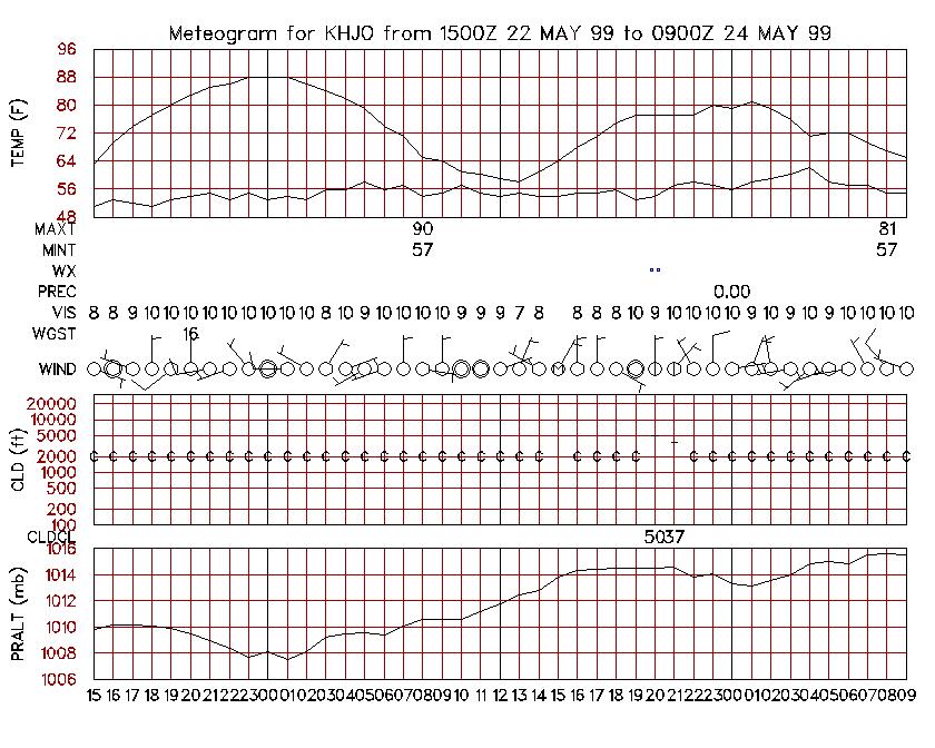
1 METR 104: Our Dynamic Weather (w/lab) Lab Exploration #4: Solar Radiation & Temperature Part I: A Simple Computer Model Dr. Dave Dempsey, Department of Earth & Climate Sciences, SFSU, Fall 2013 (5 points) (Thursday, Oct. 17) Your Name Learning Objectives. After completing this activity, you should be able to: Configure and run experiments with a simple computer model (a STELLA model) that predicts temperature at the earth's surface over a period of several days, driven by absorption of solar radiation and affected by cloud cover (but little or nothing else). Evaluate the model based on experience reading meteogram plots of observed temperature patterns and cloud cover over several days at individual locations. Begin to describe the role that computer models play in the way that science works in atmospheric science. Materials Needed. To complete this activity, you will need: A computer in TH 604 or 607 with: o STELLA modeling software installed on it, and either o a version of a STELLA model of the daily temperature cycle ("DailyTempCycle.I.STMX") or o an internet connection with a Web browser, to access the Webbased version of the model at: A graph of sun angle (in degrees) vs. time (in hours) at the latitude of Hanford, CA (36.3 N) starting on May 22 (Julian day 142) A meteogram showing a typical daily temperature cycle under cloudfree conditions at Hanford, CA (KHJO): o Ending at 09Z May 24,
2 I. Introduction. As noted in Lab #2, Part II and Lab #3, forecasting temperature is one of the most common and useful aspects of weather forecasting. Modern professional weather forecasters typically do it by starting with current and recent observations of weather conditions and applying their understanding of the underlying physical causes of temperature change, in a largely quantitative way, to estimate near-future changes in temperature from current conditions. One of the most important tools that forecasters and atmospheric scientists use is the computer model. One type of computer weather forecast and research models are based on the known physical relationships between meteorological quantities (temperature, pressure, wind speed, wind direction, humidity, etc.) and external factors that can affect them (solar radiation, topography, land vs. water surface, etc.). These relationships can be expressed mathematically and solved quantitatively using a computer, providing a forecast or scenario of the future state of the atmosphere, given a starting state. In this lab you'll configure a very simple computer model, run experiments with it, and evaluate it based on your experience reading surface weather observations displayed on meteograms. II. A Simple Computer Model of Temperature Driven by Solar Heating Our intuition is that the sun plays a central (though not necessarily the only) role in causing daily temperature variations, as we began to explore in Lab #2, Parts I and II, and Lab #3. We discovered in those labs that the intensity of solar radiation depends strongly on the angle of the sun above the horizon (sun angle), which varies with time of day and time of year at any particular location, and cloud cover also affects insolation at the earth's surface. To test the extent to which the sun (affected by variations in sun angle and cloud cover) controls the earth's surface temperature, we can build a simple computer model based on a well-established, empirical physical law called the Law of Conservation of Energy. (An empirical physical law is based on many and repeated observations of the way the physical world behaves in many, many situations.) 2
3 One version of the Law of Conservation of Energy describes how objects gain or lose heat and how the temperature of the object responds as a result. It can be written very generally like this: The rate at which an object s temperature changes is proportional to The rate at which an object s heat content changes = All of the rates at which the object gains heat by various mechanisms, added together All of the rates at which the object loses heat by various mechanisms, added together We could apply this law to the earth's surface. Moreover, if we suppose that the surface gains heat only by absorbing solar radiation, and it doesn t lose heat by any mechanism, then the Law of Conservation of Energy applied to the earth's surface would be simply: The rate at which the earth s surface temperature changes is proportional to The rate at which the heat content of a layer of the earth s surface changes = The rate at which the surface absorbs solar radiation 3
4 Using this relationship, if we know how fast the surface absorbs solar radiation, then we can calculate how fast the surface temperature changes. From that, we can estimate what the temperatures will be in the near future (if they are driven only by absorption of solar radiation). We can run this simple model, compare the results to observed daily temperature cycles, and see how well the model performs. That is, we can evaluate the model's performance. If the model does well, it could be useful for helping us understand better how the atmosphere works and perhaps even for making temperature forecasts. (To be sure, we would need more experience and further evaluation of the model.) If the model doesn't do well, we could question whether the Law Conservation of Energy applies to the earth s surface or, more likely, whether we have represented the absorption of solar radiation in the model correctly, or more likely still, whether or not we have included in the model all of the physical mechanisms by which the earth s surface gains and loses heat. 4
5 II. Instructions Respond in writing to questions posed in boxes below. Print a hard copy of the plot that you create in section D. Label the plot clearly with the details of the model run (in particular, the latitude, time of year, cloud cover, nature of the earth's surface). Turn in your written responses and plot at the end of the lab session. A. Access "Daily Temperature Cycle I", a computer model of the daily temperature cycle written using STELLA modeling software. If you are using one of the Mac computers in TH 604 or 607: 1. Make sure that there is a file called "DailyTempCycle.I.STMX" on the Desktop. (If not, alert your instructor.) 2. Locate the STELLA icon on the Dock along the bottom of the screen (a yellow disk with S at center). Click on it to start STELLA. 3. Pull down STELLA s File menu and select Open. (This opens a Chose a File: STELLA dialog window.) 4. On the left-hand side of the dialog window, under FAVORITES, select Desktop, then select the DailyTempCycle.II.A.STMX file. 5. Finally, click on the Choose button. You should now see the model interface. or, almost (but not quite) as good, if you are using a Web browser and have an internet connection, go to: Your instructor will describe the model features and explain how to configure it, run it, and access and read the graphs of model output. 5
6 B. Notice the default model configuration. In this version of the daily temperature cycle model, you can control: o Latitude (in degrees) o Day of the year (Julian day, a number from 1 to 365) o "Surface Type" (land or water) o "Cloud Cover" (as a percentage of the sky covered by clouds) If necessary, set the items above as follows (but don t run the model yet): Latitude: +36 (36 N; negative values are in the S. Hemisphere) Day of the year: 142 (Julian day, corresponding to May 22) Surface Type : 1 (1 = land, 2 = sea) Cloud Cover : 0% (no cloud cover at all) C. Make your own prediction of the daily temperature pattern, given how the sun angle varies. You have been given a plot of sun angle (in degrees) vs. time (in hours) for several days starting on May 22 at the latitude of Hanford, CA. On this plot, identify nighttime vs. daytime periods and the times of sunrise, sunset, and (solar) noon. Based on the sun angle, sketch the pattern of temperature that you would expect to see. [The actual temperatures aren't important here, just the pattern of temperature that is, the time(s) when the temperature is lowest and highest and what it does in between relative to the sun angle pattern.] 6
7 D. Run the model and compare your prediction to the model simulation. 1. Run the model (using the settings specified in Section B above). You should see the same plot of sun angle as in Step C (above) appear on the first graph (which is Page 1 of three pages of graphs). 2. View the second graph (Page 2). [Click on the lower left-hand corner of the graph, which looks as if the corner has been bent forward slightly.] This graph plots (1) the sun angle (in degrees, the blue line) and (2) temperature (in F, the red line) simulated by the model. 3. Try the following: a. place the cursor on the graph; b. click and hold the click, so that a vertical line appears on the graph through the location of the cursor; and c. drag the cursor back and forth (which drags the vertical line with it). Notice that beneath the "Hours" label along the horizontal axis you'll see the time (in hours) corresponding to the cursor's position, and beneath the "Sun Angle deg" and "Temperature F" labels along the top of the graph you'll see the values of these quantities at that hour. (Note: it works a little differently in the Web-based version.) You can use this feature to help answer some of the questions below. 7
8 Question #1: Describe any apparent correspondence that you can see between temperature (as calculated by the model) and sun angle. [For example, how does each behave at night? During daylight hours? When is temperature changing and not changing, relative to what the sun angle is or is not doing?] Question #2: In what ways is the model simulation of temperature similar to what you sketched in Step C (above)? In what ways is it different? 8
9 4. View the third graph (Page 3). It shows: (1) the rate (in Watts) at which the surface absorbs solar energy (the blue line), and (2) the temperature (in F) (the red line). For Question #3 below, you should consider surface temperature observations that you've seen plotted on meteograms (for example, on the meteograms accompanying this lab from Hanford, CA, which we first saw in Lab #2, Part II), as well as your own personal experience with the daily temperature cycle. Question #3: In what ways does the model simulation seem reasonable and in what ways does it not? 9
10 Question #4 below asks about the physical processes that are represented in the model and that determine the temperatures that the model calculates (not about the quality of the graphs that the model produces, which merely show the model output). Question #4: Do you have any suggestions about what might be done to improve the model? 5. Print a copy of only the third graph (Page 3). Label the plot clearly with the details of the model run (in particular, the latitude, time of year, cloud cover, nature of the earth's surface). To print the plot (follow these instructions carefully!): a. First, pull down STELLA's "File" menu and select "Page Setup", and next to "Orientation", select the landscape mode [the righthand icon.]. b. Then click on the printer icon in the lower left-hand corner of the graph. You'll get a "Print" dialog box. c. In the "Print" dialog box, make sure that the printer specified is "coriolis". [If coriolis isn't working, use "downpour".] d. Also in the Print dialog box, pull down the Pages menu and select Single. e. In the text box next to the Pages menu, enter 3 (for Page 3). f. Click on the Print button. g. Retrieve your plot from the printer. 10
11 E. Run the model to see if adding cloud cover or changing the nature of the earth's surface improves the simulation. 1. Specify a cloud cover greater than 50%. Don t run the model yet. Question #5: What do you predict that the temperature pattern will look like? How does your prediction differ from your first model simulation (without clouds) in Section D above? Why? 2. Run the model, and view the plots on Page 3 of the graphs. Question #6 below asks you to compare the plots on Page 3 of the graphs to those from your simulation in Section D above (where there was no cloud cover). To do this, you can address several aspects of the temperature simulations: (a) the temperature values themselves; (b) the daily temperature range from minimum to maximum; and (c) the pattern of temperature, particularly the timing of lows and highs each day and what happens in between. 11
12 Question #6: In what way(s) do your two simulations (with and without clouds) differ? Is the model simulation with clouds any better? (That is, do it's main features resemble the main features of observed daily temperature cycles more closely, such as the one observed at Hanford, CA on May 22, 1999?) 3. Specify (a) no cloud cover, but (b) change the surface type from land to ocean. Don t run the model yet. 12
13 Question #7: What do you predict the temperature pattern will look like? How does your prediction differ from your simulation in Section D above, and why? 4. Run the model, and view the plots on Page 3 of the graphs. Question #8 below asks you to compare the plots on Page 3 of the graphs to those from your simulation in Section D above (where there was also no cloud cover but the earth s surface was land, not ocean). To do this, you can address several aspects of the temperature simulations: (a) the temperature values themselves; (b) the daily temperature range from minimum to maximum; and (c) the pattern of temperature, particularly the timing of lows and highs each day and what happens in between. 13
14 Question #8: In what way(s) are your simulations over land and over ocean (both without clouds) different? Is the new simulation any better than your first simulation? 5. If you want, try increasing the cloud cover over the ocean surface to see if that helps. Good luck! 6. Turn in this lab with your written responses plus your annotated plot from Section D. 14
15 15
16 METR 104: Our Dynamic Weather (w/lab) Lab Exploration #4: Solar Radiation & Temperature Part II: A More Complex Computer Model Dr. Dave Dempsey, Department of Earth & Climate Sciences, SFSU, Fall 2013 (5 points) (Thursday, Oct. 24) Your Name Learning Objectives. After completing this activity, you should be able to: Configure a simple computer model (a STELLA model) and run experiments to calculate temperature at the earth's surface over several days, driven by absorption of solar radiation and radiative cooling. Evaluate the model, based on experience reading meteogram plots of observed daily temperature cycles at individual locations. Solidify further a description of the role that computer models play in the way that science works in atmospheric science. Materials Needed. To complete this activity, you will need: A computer in TH 604 or 607 with: o STELLA modeling software installed on it, and either o a version of a STELLA model of the daily temperature cycle ("DailyTempCycle.II.A.STMX") or o an internet connection with a Web browser, to access the Webbased version of the model at: Graphs of sun angle (in degrees) vs. time (in hours) at the latitude of Hanford, CA (36.3 N) starting on May 22 (Julian day 142) Two meteograms showing typical daily temperature cycles under cloud-free conditions at Hanford, CA (KHJO): o Ending at 07Z December 17, 1998 o Ending at 09Z May 24,
17 Prior Knowledge Required: Understanding of several forms of energy (especially sensible heat and electromagnetic radiation) Understanding of what temperature is, and the difference between temperature and heat Understanding of the Principle of Conservation of Energy, expressed in the form of a heat budget equation for an object o some ways that the earth's surface can gain and lose heat: absorption of solar radiation emission of longwave infrared radiation (others not yet accounted for) Understanding of radiative emission: o Emission as a process in which sensible heat in an object is transformed into radiative energy that propagates away (and hence a way for an object to lose heat) o How the intensity with which an object emits radiative energy depends on the object's temperature an object emits more radiative energy when it's warmer than when it's cooler (the Stefan-Boltzmann Law) o How the wavelengths of radiation that an object emits the most depend on the object's temperature an object emits most of its radiative energy at shorter wavelengths when it's hotter, and at longer wavelengths when it's colder wavelengths of emission by the sun vs. the earth (solar or shortwave radiation vs. terrestrial or longwave radiation) I. Introduction. This lab activity continues our development of a sense of how we might use (a) experience with observations and (b) basic physical principles, to understand and forecast surface temperature over the course of one to several days. In particular, it continues the development and testing of a computer model of the daily temperature cycle at the earth's surface introduced in Lab #4, Part I. In this lab you'll configure a more sophisticated version of the computer model, run experiments with it, and evaluate it based on your experience reading surface weather observations displayed on meteograms. 2
18 II. A Somewhat More Sophisticated Computer Model of Temperature Driven by Solar Heating The sun certainly plays a central (though not necessarily the only) role in controlling daily temperature variations, and clouds modify (in particular, reduce) the effect that solar radiation has on temperature during the daytime. However, we discovered in Lab #4, Part I that solar radiation alone doesn't account for some aspects of the daily temperature cycle. In particular, by accounting only for solar radiation absorption (even when modified by clouds), the temperature never falls (at night or any other time), and the temperature rises all day to a maximum at about sunset (where it stays all night), not to a maximum time in the afternoon between noon and sunset. In retrospect, the fact that the temperature never falls in that model should make sense. For an object to cool, it must lose heat. The mere absence of solar heating does not by itself give the earth's surface any way to lose heat and cool off it merely means that it's not gaining any heat and so the temperature doesn't change, as the model predicted. To overcome this shortcoming, we'll try adding emission of radiative energy to the model, a mechanism by which the earth's surface can lose heat. With this new physical processes included, the Law of Conservation of Energy applied to the earth's surface and written in a form that describes how the surface gains and loses heat and how its temperature responds as a result, can be written like this: The rate at which the earth s surface temperature changes is proportional to The rate at which the heat content of a layer of the earth s surface changes = The rate at which the surface absorbs solar radiation The rate at which the surface emits longwave infrared radiation 3
19 Using this relationship, we can calculate how fast the surface temperature changes and from that we can estimate what the temperatures will be in the near future (if they are driven by absorption of solar radiation and emission of radiative energy). We can run this somewhat more sophisticated model, compare the results to observed daily temperature cycles, and see how well the model performs. That is, we can evaluate or validate the model. If the model does well, it could be useful for helping us understand better how the atmosphere works and for making temperature forecasts. (To be sure, further experience and evaluation of the model would be necessary.) If the model doesn't do well, we have to question any assumptions that underlie the physical relationship as we've applied it (above), or perhaps take into account physical processes that are important but that we neglected. 4
20 II. Instructions Read and follow these instructions carefully. Respond in writing to questions posed in boxes below. Print a hard copy of the plot that you create in section E. Turn in your written responses and plot at the end of the lab session. A. Access "Daily Temperature Cycle II.A", a computer model of the daily temperature cycle written using STELLA modeling software. If you are using one of the Mac computers in TH 604 or 607: 1. Make sure that there is a file called "DailyTempCycle.II.A.STMX" on the Desktop. (If not, alert your instructor.) 2. Locate the STELLA icon on the Dock along the bottom of the screen (a yellow disk with S at center). Click on it to start STELLA. 3. Pull down STELLA s File menu and select Open. (This opens a Chose a File: STELLA dialog window.) 4. On the left-hand side of the dialog window, under FAVORITES, select Desktop, then select the DailyTempCycle.II.A.STMX file. 5. Finally, click on the Choose button. You should now see the model interface. or, almost (but not quite) as good, if you are using a Web browser and have an internet connection, go to: Your instructor will describe the model features and explain how to configure it, run it, and access and read the graphs of model output. Note the ways in which this model differs from the version in Lab #4, Part I. 5
21 B. Notice the default model configuration. In this version of the daily temperature cycle model, the latitude is set to 36 N (the latitude of Hanford, CA). However, you can specify: o Either of two days of the year (May 22 or December 16) o Whether or not the surface emits longwave infrared radiative energy o "Surface Type" (land or water) If necessary, set the items above as follows (but don t run the model yet): Day of the year: May 22 Emission of longwave infrared radiation: Turned off Surface Type : 1 (1 = land, 2 = sea) C. Make your own prediction of the daily temperature pattern, given how the sun angle varies. You have been given a plot of sun angle (in degrees) vs. time (in hours) for several days starting on May 22 at the latitude of Hanford, CA. On this plot, identify nighttime vs. daytime periods and the times of sunrise, sunset, and (solar) noon. Based on the sun angle, sketch the pattern of temperature that you would expect to see (assuming no clouds). [The actual temperatures aren't important here, just the pattern of temperature that is, the time(s) when the temperature is lowest and highest and what it does in between relative to the sun angle pattern.] D. Run the model and compare your prediction to the model simulation. 1. Run the model (using the settings specified in Section B above). You should see the same plot of sun angle as in Step C (above) appear on the first graph (which is Page 1 of three pages of graphs). 2. View the second graph (Page 2 of the graphs). This graph plots (1) the sun angle (in degrees, the blue line) and (2) temperature (in F, the red line) simulated by the model. 6
22 3. Try the following: a. place the cursor on the graph; b. click and hold the click, so that a vertical line appears on the graph through the location of the cursor; and c. drag the cursor back and forth (which drags the vertical line with it). Notice that beneath the "Hours" label along the horizontal axis you'll see the time (in hours) corresponding to the cursor's position, and beneath the "Sun Angle deg" and "Temperature F" labels along the top of the graph you'll see the values of these quantities at that hour. (Note: it works a little differently in the Web-based version.) 4. Rerun the model for December 16, view the second graph (Page 2 of the graphs), and notice of any differences from May 22. E. Reconfigure the model to run with radiative emission turned on, predict the results, run the model, and compare your prediction to the model simulation. 1. Turn on IR Emission and set the day of the year to May You have been given a second plot of sun angle (in degrees) vs. time (in hours) for 2.5 days (60 hours) starting on May 22 at the latitude of Hanford, CA. Based on the sun angle, sketch the pattern of temperature that you would expect to see with radiative emission turned on (again assuming no clouds). 3. Run the model and view the second graph (Page 2 of the graphs). 7
23 As before, this graph plots (1) the sun angle (in degrees, the blue line) and (2) temperature (in F, the red line) simulated by the model. Question #1: Describe any apparent correspondence that you can see between temperature (as calculated by the model) and sun angle. [For example, how does each behave at night? During daylight hours? When is temperature changing (and how fast), or not changing, relative to what the sun angle is or is not doing? (Use the cursor to help pinpoint specific temperatures and sun angles at specific times on the plot.)] 4. View the third graph (Page 3 of the graphs). It shows: (1) Blue line: The rate (in Watts) at which the surface absorbs solar energy; and (2) Red line: The temperature (in F). 8
24 For Question #2 below, you should consider surface temperature observations that you've seen plotted on meteograms (for example, on the meteograms accompanying this lab from Hanford, CA, which we first saw in Lab #2, Part II), as well as your own personal experience with the daily temperature cycle. Question #2: In what ways does the model simulation seem reasonable and in what ways does it not? 9
25 Question #3: Does the model seem to perform better than it did previously, when it calculated the effects of only solar radiation absorption? If so, how? Question #4: Are there aspects of the model prediction that don't seem to capture reality very well? If so, what? (You can rerun the model for December 16 and see if any of your observations and conclusions differ.) 10
26 5. Print a copy of only the third graph (Page 3) for the May 22 model simulation. Put your name on it, along with other information about the model simulation beyond what is already on the plot. To print the plot (follow these instructions carefully!): a. First, pull down STELLA's "File" menu and select "Page Setup", and next to "Orientation", select the landscape mode [the righthand icon.]. b. Then click on the printer icon in the lower left-hand corner of the graph. (Don t select Print from the File menu.) You should get a "Print" dialog box. c. In the "Print" dialog box, make sure that the printer specified is "coriolis". [If coriolis isn't working, use "downpour".] d. Also in the Print dialog box, pull down the Pages menu and select Single. e. In the text box next to the Pages menu, enter 3 (for Page 3). f. Click on the Print button. g. Retrieve your plot from the printer. 6. Turn in the plot along with this lab (with your written responses to Questions #1-4). 11
27 METR 104: Our Dynamic Weather (w/lab) Lab Exercise #4: Solar Radiation & Temperature Part III: An Even More Complex Computer Model Dr. Dave Dempsey, Department of Earth & Climate Sciences, SFSU, Fall 2013 (5 points) (Thursday, Nov. 7) Learning Objectives. After completing this activity, you should be able to: A. Configure and run more experiments with a simple computer model (a STELLA model) of the daily temperature cycle. B. Evaluate the model based on experience reading meteograms. C. Solidify further a description of the role that computer models play in the way that science works in atmospheric science. Materials Needed. To complete this activity, you will need: A computer in TH 604 or 607 with STELLA modeling software installed, plus either: o version III of a STELLA model of the daily temperature cycle ("DailyTempCycle.III.STM"), or o an internet connection with a Web browser, to access the Web-based version of the model at Two meteograms showing typical daily temperature cycles under cloudfree conditions at Hanford, CA (KHJO): Ending at 09Z May 24, 1999 Ending at 07Z December 17,
28 Prior Knowledge Required: Background needed for the previous lab exploration (Lab #4, Part II) Understanding of the Principle of Conservation of Energy, expressed in the form of the heat budget equation for an object, including the earth's surface o Some ways that the earth's surface can gain and lose heat: absorption of solar radiation emission of longwave infrared radiation absorption of longwave infrared radiation emitted downward by greenhouse gases and clouds conduction of heat from the surface into the atmosphere (or vice versa) evaporation of water from the earth's surface Understanding of radiative absorption: when an object absorbs radiation, the energy is transformed into (an equal amount of) sensible heat in the object II. An Even More Complex Computer Model We have been conducting a series of lab explorations to investigate ways to explain the commonly observed daily temperature cycle. In Lab #2, Part I we constructed graphs of solar radiation intensity data recorded at Hanford CA on two particular days. In Lab #2, Part II we described features of the solar radiation intensity observed at that location, and began looking for connections between the patterns of temperature and solar radiation observed there over the course of a day. In Lab #3 we looked at the meteograms for two consecutive days at two locations in Colorado and saw examples of how the weather complicates things, in particular, how factors such as cloud cover can affect the daily temperature cycle. In Lab #4, Parts I and II we began using a computer model based on the principle of conservation of energy to try to simulate observed daily temperature cycles, and to evaluate how well the model performed. The model we used in Part I (called "DailyTempCycle.I.STM") assumed that the surface temperature cycle is driven exclusively by the rate at which the surface absorbs solar radiation. We found that this model did not do a good enough job of explaining the temperature cycle. In Part II we modified the model (calling it "DailyTempCycle.II.A.STM") to take into account the fact that, in addition to absorbing solar radiation, the surface also emits longwave infrared radiation. 2
29 That last model produced a daily temperature pattern that was realistic in some ways but not in others. It produced a temperature maximum in the afternoon and cooling thereafter until near (just after) sunrise, as we commonly see in observations of the real atmosphere. The daily maximum temperature, although a little too high, wasn't too bad, but the minimum temperatures were much colder than we'd expect to see, and so the daily temperature range (the difference between the minimum and maximum temperature) was too large. We concluded that, although that model did much better than its predecessor did in Lab 4, Part I, it is likely missing one or more physical mechanisms not accounted for yet. What might those mechanisms be? We know that greenhouse gases and clouds absorb longwave infrared radiation emitted by the earth's surface. We also know that greenhouse gases and clouds emit longwave infrared radiation of their own, that they emit part of that radiation downward, and that the surface absorbs it. Hence, we'll include in the model this additional source of heat for the surface. We also know that when two objects at different temperatures are in direct contact, heat will "flow" from the warmer one to the cooler one (so the warmer one cools off and the cooler one warms up). This is the process of conduction of heat. In particular, when air in contact with the earth's surface is warmer or colder than the surface, heat will conduct from one to the other, and the surface will gain or lose heat. We'll try to represent this process in the model. Finally, we know that when water evaporates, heat in the water transforms into latent heat in the water vapor, reducing the amount of heat in the remaining water. (We experience this directly when we overheat, produce sweat, and feel cooler when the sweat evaporates from our skin.) We'll try to represent evaporative cooling in the model (especially from the oceans, less so from land). 3


%Rate% at%which%heat% conducts% between%")


 If the model doesn't do well, we have to question any assumptions that")
30 With these three new physical process added, the Law of Conservation of Energy applied to the earth's surface and written in a form that describes how the surface gains and loses heat (that is, a heat budget) and how its temperature responds as a result, can be written like this: Rate%at%which%% surface% temperature% changes% Is%propor4onal%to%% Rate%at%which% heat%content% of%a%layer%of% the%surface% changes% = % % % % % % % % % % % % % % % % % %% Rate%at%which%% surface% absorbs%solar% radia4on% "Rate%at% which%the% surface%emits% LWIR%% %Rate%at% which%surface% loses%heat%due% to%evapora4on% +%Rate%at% which%surface% absorbs%lwir% emi>ed% downward%by% greenhouse% gases% +%(or% )%Rate% at%which%heat% conducts% between% surface%and% air% Using this relationship, we can calculate how fast the surface temperature changes and estimate temperature in the near future (at least, if the model is complete and accurate). We can run this more complete model, compare the results to observed daily temperature cycles, and see how well the model performs. That is, we can evaluate, or validate, the model. If the model does well, it could be useful for helping us to understand better how the atmosphere works and for making temperature forecasts. (We'd need further experience and validation of the model to be sure.) If the model doesn't do well, we have to question any assumptions that underlie the physical relationship as we've applied it above, or perhaps take into account physical processes that are important but that we have neglected. 4
31 III. Instructions Read and follow these instructions carefully. Respond in writing to questions posed in boxes below. Print a hard copy of the plot that you create in section E. Turn in your written responses and plot at the end of the lab session. A. Access "Daily Temperature Cycle III", a computer model of the daily temperature cycle written using STELLA modeling software If you are using one of the Mac computers in TH 604 or 607: 1. Make sure that there is a file called "DailyTempCycle.III.STMX" on the Desktop. (If not, alert your instructor.) 2. Locate the STELLA icon on the Dock along the bottom of the screen (a yellow disk with S at center). Click on it to start STELLA. 3. Pull down STELLA s File menu and select Open. (This opens a Chose a File: STELLA dialog window.) 4. On the left-hand side of the dialog window, under FAVORITES, select Desktop, then select the DailyTempCycle.II.A.STMX file. 5. Finally, click on the Choose button. You should now see the model interface. or, almost (but not quite) as good, if you are using a Web browser and have an internet connection, go to: Your instructor will describe the model features and explain how to configure it, run it, and access and read the graphs of model output. Note the ways in which this model differs from the version in Lab #4, Part II. 5
32 B. Notice the default model configuration. Don't run the model yet, but note that in this version of the daily temperature cycle model you can specify: 1. Where and when the model runs: latitude (in degrees) [default: 36 N, the latitude of Hanford, CA] day of the year (Julian day, expressed as a number from 1 to 365) [default: day 142, which is May 22] 2. Whether or not each of the following ways for the surface to gain or lose heat is turned on: emission of longwave infrared radiative energy [default: turned on] absorption of longwave infrared radiation emitted downward by greenhouse gases and clouds [default: turned off] conduction of heat between the surface and the atmosphere, and evaporation of water from the surface [default: turned off] 3. Several more model parameters: "Surface Type" (land or water) [default: land] "Cloud Cover" (% of the sky covered by clouds) [default: 0%] C. Repeat a model simulation that you performed in Lab #4, Part II and confirm that is the same. (No written response required.) You have been given a plot of sun angle (in degrees) and temperature (in F) vs. time (in hours) for 2.5 days (60 hours) starting on May 22 at the latitude of Hanford, CA. (You generated this plot in Lab 4, Part II.) Run the latest version of the model with the default configuration described above, and verify that it reproduces this plot. (The plot is on the second graph, on Page 2 of the five pages of graphs available in this version of the model. Note one difference: the hours plotted along the bottom axis in this version of the model will be from 360 hours to 420 hours (15.0 to 17.5 days) instead of 0 to 60 hours (0 to 2.5 days). However, both series of times start at midnight and end at noon. Note the maximum and minimum temperatures achieved over the course of each day, and the time of day when they occur. 6
33 D. In this section we will look at the effects of (1) greenhouse gases, and (2) conduction and evaporation, on the daily temperature cycle. Respond to the questions in writing in the space provided. Before you run the model again: Question 1: How do you think that turning on greenhouse (GH) gas heating in the model will affect the temperature pattern? Turn on GH gas heating and run the model, without changing anything else. Question 2: a) Does the pattern of the daily temperature cycle change in any significant way from the previous model simulation? If so, how? b) Refer to the meteogram for Hanford, CA for the same day of the year. Do the temperatures simulated by the model (for example, the maximum and minimum values) seem more realistic, less so, or no different than, the previous model run? 7
34 Now turn on conduction/evaporation, too, and run the model again. Question 3: a) Does the pattern of the daily temperature cycle change in any significant way from the previous run? If so, how? b) Refer to the meteogram for Hanford, CA for the same day of the year. Do the temperatures simulated by the model (for example, the maximum and minimum values) seem more realistic, less so, or no different than, the previous model run? Print a copy of the graph on Page 2 of your last model run. Remember to specify that only Page 2 should be printed (not all 5 pages!). (See Lab #4, Part I or Part II for instructions about printing graphs in STELLA.) Put your name on it. Turn it in with your written responses to the questions in Sections D (above) and Section E (next page). 8
35 E. In this part you will examine the effects of clouds in the model. Before your run the model again: Question 4: If you added a significant percentage of cloud cover to the model, what do you think would happen to the daytime maximum temperature and the nighttime minimum temperature, compared to the previous model run with no cloud cover? Reconfigure the model to include significant cloud cover. Then run the model and compare the model results to your prediction. Question 5: What difference do you see in the high and low temperatures simulated by the model with cloud cover? How would you explain these results? 9
36
Lab Exploration #4: Solar Radiation & Temperature Part II: A More Complex Computer Model
 METR 104: Our Dynamic Weather (w/lab) Lab Exploration #4: Solar Radiation & Temperature Part II: A More Complex Computer Model Dr. Dave Dempsey, Department of Earth & Climate Sciences, SFSU, Spring 2014
Lab Exercise #2: Solar Radiation & Temperature Part VI: An Even More Complex Computer Model
 METR 104: Our Dynamic Weather (w/lab) Lab Exercise #2: Solar Radiation & Temperature Part VI: An Even More Complex Computer Model Dr. Dave Dempsey Dept. of Geosciences Dr. Oswaldo Garcia, & Denise Balukas
Lab Exploration #5: The Weather Complicates Things Further. Learning Objectives. After completing this activity, you should be able to:
 METR 104: Our Dynamic Weather (w/lab) Lab Exploration #5: The Weather Complicates Things Further Dr. Dave Dempsey, Department of Earth & Climate Sciences, SFSU, Spring 2014 (5 points) (Thursday, April
Solutions to Lab Exercise #2: Solar Radiation & Temperature Part II: Exploring & Interpreting Data
 METR 104: Our Dynamic Weather (w/lab) Solutions to Lab Exercise #2: Solar Radiation & Temperature Part II: Exploring & Interpreting Data (10 points) Dr. Dave Dempsey Dept. of Geosciences SFSU, Spring 2013
Earth s Energy Budget: How Is the Temperature of Earth Controlled?
 1 NAME Investigation 2 Earth s Energy Budget: How Is the Temperature of Earth Controlled? Introduction As you learned from the reading, the balance between incoming energy from the sun and outgoing energy
Name(s) Period Date. Earth s Energy Budget: How Is the Temperature of Earth Controlled?
 Period Date. Earth s Energy Budget: How Is the Temperature of Earth Controlled?") Name(s) Period Date 1 Introduction Earth s Energy Budget: How Is the Temperature of Earth Controlled? As you learned from the reading, the balance between incoming energy from the sun and outgoing energy
Name(s) Period Date 1 Introduction Earth s Energy Budget: How Is the Temperature of Earth Controlled? As you learned from the reading, the balance between incoming energy from the sun and outgoing energy
Lecture # 04 January 27, 2010, Wednesday Energy & Radiation
 Lecture # 04 January 27, 2010, Wednesday Energy & Radiation Kinds of energy Energy transfer mechanisms Radiation: electromagnetic spectrum, properties & principles Solar constant Atmospheric influence
FOLLOW THE ENERGY! EARTH S DYNAMIC CLIMATE SYSTEM
 Investigation 1B FOLLOW THE ENERGY! EARTH S DYNAMIC CLIMATE SYSTEM Driving Question How does energy enter, flow through, and exit Earth s climate system? Educational Outcomes To consider Earth s climate
AT350 EXAM #1 September 23, 2003
 AT350 EXAM #1 September 23, 2003 Name and ID: Enter your name and student ID number on the answer sheet and on this exam. Record your answers to the questions by using a No. 2 pencil to completely fill
The inputs and outputs of energy within the earth-atmosphere system that determines the net energy available for surface processes is the Energy
 Energy Balance The inputs and outputs of energy within the earth-atmosphere system that determines the net energy available for surface processes is the Energy Balance Electromagnetic Radiation Electromagnetic
Lecture 4: Heat, and Radiation
 Lecture 4: Heat, and Radiation Heat Heat is a transfer of energy from one object to another. Heat makes things warmer. Heat is measured in units called calories. A calorie is the heat (energy) required
Lecture 2: Global Energy Cycle
 Lecture 2: Global Energy Cycle Planetary energy balance Greenhouse Effect Vertical energy balance Solar Flux and Flux Density Solar Luminosity (L) the constant flux of energy put out by the sun L = 3.9
Lecture 5: Greenhouse Effect
 Lecture 5: Greenhouse Effect S/4 * (1-A) T A 4 T S 4 T A 4 Wien s Law Shortwave and Longwave Radiation Selected Absorption Greenhouse Effect Global Energy Balance terrestrial radiation cooling Solar radiation
Sunlight and Temperature
 Sunlight and Temperature Name Purpose: Study microclimate differences due to sunlight exposure, location, and surface; practice environmental measurements; study natural energy flows; compare measurements;
Lecture 5: Greenhouse Effect
 /30/2018 Lecture 5: Greenhouse Effect Global Energy Balance S/ * (1-A) terrestrial radiation cooling Solar radiation warming T S Global Temperature atmosphere Wien s Law Shortwave and Longwave Radiation
Assignment #0 Using Stellarium
 Name: Class: Date: Assignment #0 Using Stellarium The purpose of this exercise is to familiarize yourself with the Stellarium program and its many capabilities and features. Stellarium is a visually beautiful
Lecture 2: Global Energy Cycle
 Lecture 2: Global Energy Cycle Planetary energy balance Greenhouse Effect Selective absorption Vertical energy balance Solar Flux and Flux Density Solar Luminosity (L) the constant flux of energy put out
Solar Flux and Flux Density. Lecture 2: Global Energy Cycle. Solar Energy Incident On the Earth. Solar Flux Density Reaching Earth
 Lecture 2: Global Energy Cycle Solar Flux and Flux Density Planetary energy balance Greenhouse Effect Selective absorption Vertical energy balance Solar Luminosity (L) the constant flux of energy put out
Chapter 2 Solar and Infrared Radiation
 Chapter 2 Solar and Infrared Radiation Chapter overview: Fluxes Energy transfer Seasonal and daily changes in radiation Surface radiation budget Fluxes Flux (F): The transfer of a quantity per unit area
Electromagnetic Radiation. Radiation and the Planetary Energy Balance. Electromagnetic Spectrum of the Sun
 Radiation and the Planetary Energy Balance Electromagnetic Radiation Solar radiation warms the planet Conversion of solar energy at the surface Absorption and emission by the atmosphere The greenhouse
Infrared Experiments of Thermal Energy and Heat Transfer
 Infrared Experiments of Thermal Energy and Heat Transfer You will explore thermal energy, thermal equilibrium, heat transfer, and latent heat in a series of hands-on activities augmented by the thermal
Today s AZ Daily Star has 2 interesting articles: one on our solar future & the other on an issue re: our state-mandated energy-efficiency plan
 REMINDER Water topic film Today s AZ Daily Star has 2 interesting articles: one on our solar future & the other on an issue re: our state-mandated energy-efficiency plan Find out all about solar in Arizona
I. Objectives Describe vertical profiles of pressure in the atmosphere and ocean. Compare and contrast them.
 ERTH 430: Lab #1: The Vertical Dr. Dave Dempsey Fluid Dynamics Pressure Gradient Force/Mass Earth & Clim. Sci. in Earth Systems SFSU, Fall 2016 (Tuesday, Oct. 25; 5 pts) I. Objectives Describe vertical
Name... Class... Date...
 Radiation and temperature Specification reference: P6.3 Black body radiation (physics only) Aims This is an activity that has been designed to help you improve your literacy skills. In this activity you
Earth s Energy Balance and the Atmosphere
 Earth s Energy Balance and the Atmosphere Topics we ll cover: Atmospheric composition greenhouse gases Vertical structure and radiative balance pressure, temperature Global circulation and horizontal energy
Chapter 2. Heating Earth's Surface & Atmosphere
 Chapter 2 Heating Earth's Surface & Atmosphere Topics Earth-Sun Relationships Energy, Heat and Temperature Mechanisms of Heat Transfer What happens to Incoming Solar Radiation? Radiation Emitted by the
Energy Balance and Temperature. Ch. 3: Energy Balance. Ch. 3: Temperature. Controls of Temperature
 Energy Balance and Temperature 1 Ch. 3: Energy Balance Propagation of Radiation Transmission, Absorption, Reflection, Scattering Incoming Sunlight Outgoing Terrestrial Radiation and Energy Balance Net
Energy Balance and Temperature
 Energy Balance and Temperature 1 Ch. 3: Energy Balance Propagation of Radiation Transmission, Absorption, Reflection, Scattering Incoming Sunlight Outgoing Terrestrial Radiation and Energy Balance Net
ATS150 Global Climate Change Spring 2019 Candidate Questions for Exam #1
 1. How old is the Earth? About how long ago did it form? 2. What are the two most common gases in the atmosphere? What percentage of the atmosphere s molecules are made of each gas? 3. About what fraction
Global Climate Change
 Global Climate Change Definition of Climate According to Webster dictionary Climate: the average condition of the weather at a place over a period of years exhibited by temperature, wind velocity, and
Temperature (T) degrees Celsius ( o C) arbitrary scale from 0 o C at melting point of ice to 100 o C at boiling point of water Also (Kelvin, K) = o C
 degrees Celsius ( o C) arbitrary scale from 0 o C at melting point of ice to 100 o C at boiling point of water Also (Kelvin, K) = o C") 1 2 3 4 Temperature (T) degrees Celsius ( o C) arbitrary scale from 0 o C at melting point of ice to 100 o C at boiling point of water Also (Kelvin, K) = o C plus 273.15 0 K is absolute zero, the minimum
1 2 3 4 Temperature (T) degrees Celsius ( o C) arbitrary scale from 0 o C at melting point of ice to 100 o C at boiling point of water Also (Kelvin, K) = o C plus 273.15 0 K is absolute zero, the minimum
Lecture 4: Radiation Transfer
 Lecture 4: Radiation Transfer Spectrum of radiation Stefan-Boltzmann law Selective absorption and emission Reflection and scattering Remote sensing Importance of Radiation Transfer Virtually all the exchange
Clouds and Rain Unit (3 pts)
") Name: Section: Clouds and Rain Unit (Topic 8A-2) page 1 Clouds and Rain Unit (3 pts) As air rises, it cools due to the reduction in atmospheric pressure Air mainly consists of oxygen molecules and nitrogen
Name: Section: Clouds and Rain Unit (Topic 8A-2) page 1 Clouds and Rain Unit (3 pts) As air rises, it cools due to the reduction in atmospheric pressure Air mainly consists of oxygen molecules and nitrogen
CLIMATE AND CLIMATE CHANGE MIDTERM EXAM ATM S 211 FEB 9TH 2012 V1
 CLIMATE AND CLIMATE CHANGE MIDTERM EXAM ATM S 211 FEB 9TH 2012 V1 Name: Student ID: Please answer the following questions on your Scantron Multiple Choice [1 point each] (1) The gases that contribute to
Temperature AOSC 200 Tim Canty
 Temperature AOSC 200 Tim Canty Class Web Site: http://www.atmos.umd.edu/~tcanty/aosc200 Topics for today: Daily Temperatures Role of clouds, latitude, land/water Lecture 09 Feb 26 2019 1 Today s Weather
Warming Earth and its Atmosphere The Diurnal and Seasonal Cycles
 Warming Earth and its Atmosphere The Diurnal and Seasonal Cycles Or, what happens to the energy received from the sun? First We Need to Understand The Ways in Which Heat Can be Transferred in the Atmosphere
Lecture Outlines PowerPoint. Chapter 16 Earth Science 11e Tarbuck/Lutgens
 Lecture Outlines PowerPoint Chapter 16 Earth Science 11e Tarbuck/Lutgens 2006 Pearson Prentice Hall This work is protected by United States copyright laws and is provided solely for the use of instructors
G109 Alternate Midterm Exam October, 2004 Instructor: Dr C.M. Brown
 1 Time allowed 50 mins. Answer ALL questions Total possible points;50 Number of pages:8 Part A: Multiple Choice (1 point each) [total 24] Answer all Questions by marking the corresponding number on the
Chapter 3. Multiple Choice Questions
 Chapter 3 Multiple Choice Questions 1. In the case of electromagnetic energy, an object that is hot: a. radiates much more energy than a cool object b. radiates much less energy than a cool object c. radiates
Composition, Structure and Energy. ATS 351 Lecture 2 September 14, 2009
 Composition, Structure and Energy ATS 351 Lecture 2 September 14, 2009 Composition of the Atmosphere Atmospheric Properties Temperature Pressure Wind Moisture (i.e. water vapor) Density Temperature A measure
COMPUTER METHODS AND MODELING IN GEOLOGY MODELING EARTH'S TEMPERATURE
 COMPUTER METHODS AND MODELING IN GEOLOGY MODELING EARTH'S TEMPERATURE The parts of this exercise for students are in normal text, whereas answers and explanations for faculty are italicized. In this week's
Earth is tilted (oblique) on its Axis!
 on its Axis!") MONDAY AM Radiation, Atmospheric Greenhouse Effect Earth's orbit around the Sun is slightly elliptical (not circular) Seasons & Days Why do we have seasons? Why aren't seasonal temperatures highest at
MONDAY AM Radiation, Atmospheric Greenhouse Effect Earth's orbit around the Sun is slightly elliptical (not circular) Seasons & Days Why do we have seasons? Why aren't seasonal temperatures highest at
Energy: Warming the earth and Atmosphere. air temperature. Overview of the Earth s Atmosphere 9/10/2012. Composition. Chapter 3.
 Overview of the Earth s Atmosphere Composition 99% of the atmosphere is within 30km of the Earth s surface. N 2 78% and O 2 21% The percentages represent a constant amount of gas but cycles of destruction
Mon Oct 20. Today: radiation and temperature (cont) sun-earth geometry energy balance >> conceptual model of climate change Tues:
 sun-earth geometry energy balance >> conceptual model of climate change Tues:") Mon Oct 20 Announcements: bring calculator to class from now on > in-class activities > midterm and final Today: radiation and temperature (cont) sun-earth geometry energy balance >> conceptual model of
Mon Oct 20 Announcements: bring calculator to class from now on > in-class activities > midterm and final Today: radiation and temperature (cont) sun-earth geometry energy balance >> conceptual model of
Students will explore Stellarium, an open-source planetarium and astronomical visualization software.
 page 22 STELLARIUM* OBJECTIVE: Students will explore, an open-source planetarium and astronomical visualization software. BACKGROUND & ACKNOWLEDGEMENTS This lab was generously provided by the Red Rocks
Topic # 12 How Climate Works
 Topic # 12 How Climate Works A Primer on How the Energy Balance Drives Atmospheric & Oceanic Circulation, Natural Climatic Processes pp 63-68 in Class Notes How do we get energy from this........ to drive
- matter-energy interactions. - global radiation balance. Further Reading: Chapter 04 of the text book. Outline. - shortwave radiation balance
 (1 of 12) Further Reading: Chapter 04 of the text book Outline - matter-energy interactions - shortwave radiation balance - longwave radiation balance - global radiation balance (2 of 12) Previously, we
MATH 392, Seminar in Mathematics and Climate Computer Project #1: Energy Balance Models
 MATH 392, Seminar in Mathematics and Climate Computer Project #1: Energy Balance Models DUE DATE: Thursday, Feb. 1, 2018 The goal of this project is for you to investigate the Earth s climate using some
ATMOSPHERIC ENERGY and GLOBAL TEMPERATURES. Physical Geography (Geog. 300) Prof. Hugh Howard American River College
 Prof. Hugh Howard American River College") ATMOSPHERIC ENERGY and GLOBAL TEMPERATURES Physical Geography (Geog. 300) Prof. Hugh Howard American River College RADIATION FROM the SUN SOLAR RADIATION Primarily shortwave (UV-SIR) Insolation Incoming
ATMOSPHERIC ENERGY and GLOBAL TEMPERATURES Physical Geography (Geog. 300) Prof. Hugh Howard American River College RADIATION FROM the SUN SOLAR RADIATION Primarily shortwave (UV-SIR) Insolation Incoming
1. Which continents are experiencing daytime? 2. Which continents are experiencing nighttime?
 Name: Section: Astronomy 101: Seasons Lab Objective: When you have completed this lab, you will be able to describe the seasons of the year and explain the reasons for those seasons. Answer the questions
GC 170A1 INTRO TO GLOBAL CHANGE MIDTERM STUDY GUIDE Fall 2014
 GC 170A1 INTRO TO GLOBAL CHANGE MIDTERM STUDY GUIDE Fall 2014 FORMAT OF THE EXAM: The exam is worth 200 points and will consist of questions in a variety of formats: multiple choice questions (about 25
Global Energy Balance Climate Model. Dr. Robert M. MacKay Clark College Physics & Meteorology
 Global Energy Balance Climate Model Dr. Robert M. MacKay Clark College Physics & Meteorology rmackay@clark.edu (note: the value of 342 W/m 2 given in this figure is the solar constant divided by 4.0 (1368/4.0).
Meteorology Pretest on Chapter 2
 Meteorology Pretest on Chapter 2 MULTIPLE CHOICE 1. The earth emits terrestrial radiation a) only at night b) all the time c) only during winter d) only over the continents 2. If an imbalance occurs between
Energy, Temperature, & Heat. Energy, Temperature, & Heat. Temperature Scales 1/17/11
 Energy, Temperature, & Heat Energy is the ability to do work (push, pull, lift) on some form of matter. Chapter 2 Potential energy is the potential for work (mass x gravity x height) Kinetic energy is
In this activity, students will compare weather data from to determine if there is a warming trend in their community.
 Overview: In this activity, students will compare weather data from 1910-2000 to determine if there is a warming trend in their community. Objectives: The student will: use the Internet to locate scientific
Spectrum of Radiation. Importance of Radiation Transfer. Radiation Intensity and Wavelength. Lecture 3: Atmospheric Radiative Transfer and Climate
 Lecture 3: Atmospheric Radiative Transfer and Climate Radiation Intensity and Wavelength frequency Planck s constant Solar and infrared radiation selective absorption and emission Selective absorption
Laboratory Exercise #7 - Introduction to Atmospheric Science: The Seasons
 Laboratory Exercise #7 - Introduction to Atmospheric Science: The Seasons page - 1 Section A - Introduction: This lab consists of both computer-based and noncomputer-based questions dealing with atmospheric
Lecture 3: Atmospheric Radiative Transfer and Climate
 Lecture 3: Atmospheric Radiative Transfer and Climate Solar and infrared radiation selective absorption and emission Selective absorption and emission Cloud and radiation Radiative-convective equilibrium
International Conference on Climate Change natural greenhouse effect radiative transfer model
 One of the points that Dr. Richard Lindzen made during his keynote speech at the 2nd International Conference on Climate Change, held in New York City March 8-10 this year, is that we global warming skeptics
Torben Königk Rossby Centre/ SMHI
 Fundamentals of Climate Modelling Torben Königk Rossby Centre/ SMHI Outline Introduction Why do we need models? Basic processes Radiation Atmospheric/Oceanic circulation Model basics Resolution Parameterizations
Teaching the Greenhouse Effect. Brian Hornbuckle and Ray Arritt
 Teaching the Greenhouse Effect Brian Hornbuckle and Ray Arritt It is true that there are other factors (such as volcanic activity, variations in the earth s orbit and axis, the solar cycle), yet a number
Chapter 2--Warming the Earth and the Atmosphere
 Chapter 2--Warming the Earth and the Atmosphere Student: 1. Which of the following provides a measure of the average speed of air molecules? A. pressure B. temperature C. density D. heat 2. A change of
Topic # 10 THE EARTH S GLOBAL ENERGY BALANCE
 Topic # 10 THE EARTH S GLOBAL ENERGY BALANCE Applying the laws, etc. to understand how processes all work together to create global weather & climate!! BOOKMARK pp 51 & 115 BOOKMARK pp 51 & 115 in Class
GE510 Physical Principles of the Envt
 GE510 Physical Principles of the Envt Earth s Energy Balance: 1. Types and key properties of energy 2. Blackbody radiation revisited and Wein s displacement law 3. Transformations of the sun s radiant
GEOGRAPHY EYA NOTES. Weather. atmosphere. Weather and climate
 GEOGRAPHY EYA NOTES Weather and climate Weather The condition of the atmosphere at a specific place over a relatively short period of time Climate The atmospheric conditions of a specific place over a
,Solar Energy, Greenhouse effect, Convection.notebook October 31, 2016
 Essential Question: How is weather created? What is Solar Energy? The driving source of energy for Earth. 1. Heats Earth's land, water, and air. 2. Causes movement in the atmosphere. Key Topics: The sun
Planetary Atmospheres: Earth and the Other Terrestrial Worlds Pearson Education, Inc.
 Planetary Atmospheres: Earth and the Other Terrestrial Worlds 10.1 Atmospheric Basics Our goals for learning: What is an atmosphere? How does the greenhouse effect warm a planet? Why do atmospheric properties
Understanding the Greenhouse Effect
 EESC V2100 The Climate System spring 200 Understanding the Greenhouse Effect Yochanan Kushnir Lamont Doherty Earth Observatory of Columbia University Palisades, NY 1096, USA kushnir@ldeo.columbia.edu Equilibrium
Lecture 3: Global Energy Cycle
 Lecture 3: Global Energy Cycle Planetary energy balance Greenhouse Effect Vertical energy balance Latitudinal energy balance Seasonal and diurnal cycles Solar Flux and Flux Density Solar Luminosity (L)
Atmospheric Radiation
 Atmospheric Radiation NASA photo gallery Introduction The major source of earth is the sun. The sun transfer energy through the earth by radiated electromagnetic wave. In vacuum, electromagnetic waves
Lecture 14 - Radiative equilibrium and the atmospheric greenhouse effect
 We now have most of the tools we will need to begin to study energy balance on the earth. It will be a balance between incoming sunlight energy and outgoing energy emitted by the earth. We will look at
MASSACHUSETTS INSTITUTE OF TECHNOLOGY Department of Physics Problem Solving 10: The Greenhouse Effect. Section Table and Group
 MASSACHUSETTS INSTITUTE OF TECHNOLOGY Department of Physics 8.02 Problem Solving 10: The Greenhouse Effect Section Table and Group Names Hand in one copy per group at the end of the Friday Problem Solving
ESS15 Lecture 7. The Greenhouse effect.
 ESS15 Lecture 7 The Greenhouse effect. Housekeeping. First midterm is in one week. Open book, open notes. Covers material through end of Friday s lecture Including today s lecture (greenhouse effect) And
Modeling Daisyworld. Introduction
 Modeling Daisyworld Introduction Modeling Daisyworld Planetary Temperature Solar Luminosity Planetary Albedo Growth of Daisies Model Diagram Model Equations Experiments RETURN TO MAIN PAGE Introduction
Directed Reading. Section: Solar Energy and the Atmosphere RADIATION. identical point on the next wave. waves
 Skills Worksheet Directed Reading Section: Solar Energy and the Atmosphere 1. How is Earth s atmosphere heated? 2. Name the two primary sources of heat in the atmosphere. RADIATION In the space provided,
Radiation in the atmosphere
 Radiation in the atmosphere Flux and intensity Blackbody radiation in a nutshell Solar constant Interaction of radiation with matter Absorption of solar radiation Scattering Radiative transfer Irradiance
Bring a printed copy of this lab to your lab section. We will answer the lettered questions in class.
 Lab 2 GEO 302C Week of January 30, 2006. Bring a printed copy of this lab to your lab section. We will answer the lettered questions in class. Goal for today: Be able to understand the greenhouse effect
Lecture 9: Climate Sensitivity and Feedback Mechanisms
 Lecture 9: Climate Sensitivity and Feedback Mechanisms Basic radiative feedbacks (Plank, Water Vapor, Lapse-Rate Feedbacks) Ice albedo & Vegetation-Climate feedback Cloud feedback Biogeochemical feedbacks
Introduction to Astronomy Laboratory Exercise #1. Intro to the Sky
 Introduction to Astronomy Laboratory Exercise #1 Partners Intro to the Sky Date Section Purpose: To develop familiarity with the daytime and nighttime sky through the use of Stellarium. Equipment: Computer
Lecture 6. Solar vs. terrestrial radiation and the bare rock climate model.
 Lecture 6 Solar vs. terrestrial radiation and the bare rock climate model. Radiation Controls energy balance of Earth Is all around us all the time. Can be labeled by its source (solar, terrestrial) or
A) usually less B) dark colored and rough D) light colored with a smooth surface A) transparency of the atmosphere D) rough, black surface
 usually less B) dark colored and rough D) light colored with a smooth surface A) transparency of the atmosphere D) rough, black surface") 1. Base your answer to the following question on the diagram below which shows two identical houses, A and B, in a city in North Carolina. One house was built on the east side of a factory, and the other
1. Base your answer to the following question on the diagram below which shows two identical houses, A and B, in a city in North Carolina. One house was built on the east side of a factory, and the other
Evaluation copy. Ground Temperature Measurements. computer OBJECTIVES MATERIALS PRE-LAB QUESTIONS
 Ground Temperature Measurements Computer P3 Throughout the daylight hours the sun heats up the air and the soil. Project 1 in this manual investigates the changes in air temperature during this process.
Kinds of Energy. Defining Energy is Hard! EXPLAIN: 1. Energy and Radiation. Conservation of Energy. Sco; Denning CSU ESMEI ATS 1
 Defining Energy is Hard! EXPLAIN: 1. Energy and Radiation Energy is the capacity to perform work (but physicists have a special definition for work, too!) Part of the trouble is that scientists have appropriated
CHEMISTRY SEMESTER ONE
 EMISSION SPECTROSCOPY Lab format: this lab is a remote lab activity Relationship to theory: This activity covers the relationship between colors and absorbed/emitted light, as well as the relationship
1. Weather and climate.
 Lecture 31. Introduction to climate and climate change. Part 1. Objectives: 1. Weather and climate. 2. Earth s radiation budget. 3. Clouds and radiation field. Readings: Turco: p. 320-349; Brimblecombe:
Chapter 11 Lecture Outline. Heating the Atmosphere
 Chapter 11 Lecture Outline Heating the Atmosphere They are still here! Focus on the Atmosphere Weather Occurs over a short period of time Constantly changing Climate Averaged over a long period of time
Albedo and Heat Absorption
 In this experiment, we will be delving into the world of reflection and absorption. As light energy hits different surfaces, some of the light energy is reflected, while most of the rest of the light is
COURSE CLIMATE SCIENCE A SHORT COURSE AT THE ROYAL INSTITUTION
 COURSE CLIMATE SCIENCE A SHORT COURSE AT THE ROYAL INSTITUTION DATE 4 JUNE 2014 LEADER CHRIS BRIERLEY Course Outline 1. Current climate 2. Changing climate 3. Future climate change 4. Consequences 5. Human
Blackbody Radiation. A substance that absorbs all incident wavelengths completely is called a blackbody.
 Blackbody Radiation A substance that absorbs all incident wavelengths completely is called a blackbody. What's the absorption spectrum of a blackbody? Absorption (%) 100 50 0 UV Visible IR Wavelength Blackbody
Atmospheric "greenhouse effect" - How the presence of an atmosphere makes Earth's surface warmer
 Atmospheric "greenhouse effect" - How the presence of an atmosphere makes Earth's surface warmer Some relevant parameters and facts (see previous slide sets) (So/) 32 W m -2 is the average incoming solar
Earth s Atmosphere. Energy Transfer in the Atmosphere. 3. All the energy from the Sun reaches Earth s surface.
 CHAPTER 11 LESSON 2 Earth s Atmosphere Energy Transfer in the Atmosphere Key Concepts How does energy transfer from the Sun to Earth and to the atmosphere? How are air circulation patterns within the atmosphere
Lecture 4: Global Energy Balance
 Lecture : Global Energy Balance S/ * (1-A) T A T S T A Blackbody Radiation Layer Model Greenhouse Effect Global Energy Balance terrestrial radiation cooling Solar radiation warming Global Temperature atmosphere
GARP 0102 Earth Radiation Balance (Part 1)
") Class 8: Earth s Radiation Balance I (Chapter 4) 1. Earth s Radiation Balance: Sun, Atmosphere, and Earth s Surface as a System 2. Electromagnetic Radiation: Shortwave vs. longwave radiation (Page 69-71)
Class 8: Earth s Radiation Balance I (Chapter 4) 1. Earth s Radiation Balance: Sun, Atmosphere, and Earth s Surface as a System 2. Electromagnetic Radiation: Shortwave vs. longwave radiation (Page 69-71)
Lecture 4: Global Energy Balance. Global Energy Balance. Solar Flux and Flux Density. Blackbody Radiation Layer Model.
 Lecture : Global Energy Balance Global Energy Balance S/ * (1-A) terrestrial radiation cooling Solar radiation warming T S Global Temperature Blackbody Radiation ocean land Layer Model energy, water, and
Questions you should be able to answer after reading the material
 Module 4 Radiation Energy of the Sun is of large importance in the Earth System, it is the external driving force of the processes in the atmosphere. Without Solar radiation processes in the atmosphere
Course Outline CLIMATE SCIENCE A SHORT COURSE AT THE ROYAL INSTITUTION. 1. Current climate. 2. Changing climate. 3. Future climate change
 COURSE CLIMATE SCIENCE A SHORT COURSE AT THE ROYAL INSTITUTION DATE 4 JUNE 2014 LEADER CHRIS BRIERLEY Course Outline 1. Current climate 2. Changing climate 3. Future climate change 4. Consequences 5. Human
Arctice Engineering Module 3a Page 1 of 32
 Welcome back to the second part of the second learning module for Fundamentals of Arctic Engineering online. We re going to review in this module the fundamental principles of heat transfer. Exchange of
2/22/ Atmospheric Characteristics
 17.1 Atmospheric Characteristics Atmosphere: the gaseous layer that surrounds the Earth I. In the past, gases came from volcanic eruptions A. Water vapor was a major component of outgassing B. Other gases
Sea Ice and Satellites
 Sea Ice and Satellites Overview: Students explore satellites: what they are, how they work, how they are used, and how to interpret satellite images of sea ice using Google Earth. (NOTE: This lesson may
SIT IN YOUR GROUP AREA TODAY!
 Tuesday Sep 23th SIT IN YOUR GROUP AREA TODAY! Wrap-Up of Topic #5 on the Radiation Laws to get ready for Topic # 6 Atmospheric & Structure & Composition RQ-3 was cutoff 30 minutes before class today if