STATISTICAL MODELING OF VIDEO EVENT MINING. A dissertation presented to. the faculty of

Transcription

1 STATISTICAL MODELING OF VIDEO EVENT MINING A dissertation presented to the faculty of the Russ College of Engineering and Technology of Ohio University In partial fulfillment of the requirements for the degree Doctor of Philosophy Limin Ma June 2006

2 This dissertation entitled STATISTICAL MODELING OF VIDEO EVENT MINING by LIMIN MA has been approved for the School of Electrical Engineering and Computer Science and the Russ College of Engineering and Technology by David M. Chelberg Associate Professor of Electrical Engineering and Computer Science Dennis Irwin Dean, Russ College of Engineering and Technology

3 MA, LIMIN, Ph.D., June 2006, Electrical Engineering and Computer Science STATISTICAL MODELING OF VIDEO EVENT MINING 166 pp. Director of Dissertation: David M. Chelberg Video events contain rich semantic information. Using computational approaches to analyze video events is very important for many applications due to the desire to interpret digital data in a way that is consistent with human knowledge. This thesis investigates object-based video event analysis based on a statistical framework. Within the proposed architecture for object-based video event understanding, object detection is addressed by model-based approaches with the integration of prior color/shape knowledge and recognition feedback. Object classification is investigated as shape-based image retrieval. The relevance feedback is used to adaptively derive basis vectors to capture a user s perceptual preferences. The major focus of this thesis is concerned with statistical modeling of facial event recognition. Two hidden Markov model HMM based approaches are presented. The first approach tracks the deformation of facial components in image sequences via active shape models ASMs and extracts geometric-based features for facial gestures. The interaction between upper and lower facial components is explicitly modeled via coupled HMMs CHMMs by introducing coupled dependencies between hidden variables. The second approach automatically locates face regions in each image frame via eigenanalysis, extracts multi-band appearance features based on Gabor filtering, and models the spatio-temporal stochastic structure of facial image sequences using hierarchical HMMs HHMMs.

4 The major contributions of this thesis include: 1 a fully automatic person-independent facial expression recognition prototype system; 2 modeling of the spatio-temporal structure of facial image sequences within a hierarchical framework; 3 derived generalized inference and learning algorithms of HHMMs for observation sequences with known multiscale structures; 4 improved performance of ASMs for facial component tracking by using dynamic programming based search with contextual constraints; 5 explicit modeling of the interaction between upper and lower facial components via CHMMs for facial gesture recognition. The proposed architecture provides a feasible method for object-based video event analysis. In particular, the proposed statistical models provide more accurate modeling schemes than conventional HMMs for characterizing facial image sequences and experimentally demonstrate their advantages for facial gesture/expression recognition. Although only demonstrated on the problem of facial event recognition, the proposed approach can be extended to general video event understanding. Approved: David M. Chelberg Associate Professor of Electrical Engineering and Computer Science

5 5 ACKNOWLEDGMENTS First and most of all, I would like to express my deepest gratitude to my advisor, Prof. David M. Chelberg for his constant support, insightful guidance and kindly encouragement throughout the past four years of study and research. The support from other advisory committee members, Prof. Cynthia Marling, Prof. Jeffery Dill, Prof. Jungdong Liu and Prof. Martin Mohlenkamp, is also gratefully acknowledged and appreciated. Special thanks are given to Prof. Mehmet Celenk for his advice and collaboration in my doctoral research. I would also like to take this opportunity to thank both my friends and fellow graduate students for their assistance and suggestions. They are Dr. Qiang Zhou, Min Zhou, Mark Goldman, Mark Tomko, Heather Biggs, Tom Ruch, and Nathan Welch. I am also grateful to the unconditioned support and understanding from my wife and my family, without whose support, this thesis work is impossible in many ways.

6 6 TABLE OF CONTENTS Page Abstract Acknowledgments List of Figures List of Tables Introduction Background Challenges Generic Architecture Major Contributions Thesis Organization Literature Review Object Detection Object Classification Moving Object Tracking Object-based Semantic Event Modeling Model-based Object Detection Active Contours with Color, Texture and Shape Priors Gradient Vector Flow Active Contour Models Color and Texture Potential Field Shape Potential Field Vector Flow Field Integration Adaptive Object Detection via Recognition Feedback Object Recognition based on Markov Random Fields Confidence Map Optimization Process Shape-based Object Classification via Retrieval Introduction Algorithm Shape descriptor Linear Discriminant Analysis Relevance Feedback and LDA Adaptation

7 7 4.3 Experimental Results Conclusions Statistical Modeling of Temporal Events Hidden Markov Models Model Description Inference and Learning Coupled Hidden Markov Models Model Description Parameter Estimation Inference Problem Hierarchical Hidden Markov Models Model Definition Probabilistic Inference and Parameter Estimation The Evaluation Algorithms The Generalized Viterbi Decoding Algorithm The Estimation Algorithm Computational Complexity Facial Event Understanding in Image Sequences Related Work Facial Gesture Recognition Using Active Shape Models and Coupled HMMs Active Shape Models Experimental Results Conclusions Spatio-temporal Modeling of Facial Expression using Gabor Wavelets and Hierarchial Hidden Markov Models Face Localization Feature Extraction based on Gabor Filtering Experimental Results Conclusions Conclusions and Future Work Bibliography

8 LIST OF FIGURES 1.1 Generic architecture of object-based video event mining Structure of event modeling Potential field and vector flow field generated by color and texture priors. Courtesy of Dr. Zhou [1] Vector flow field based on the longest and shortest Radon transform. Courtesy of Dr. Zhou [1] Model-based image segmentation results. Courtesy of Dr. Zhou [1] Feedback Architecture. Courtesy of Dr. Zhou [1] Concept of Confidence Map. Courtesy of Dr. Zhou [1] Confidence map of a real scene and optimization result of a real scene. Courtesy of Dr. Zhou [1] PCA vs. LDA for subjective separability The diagram of LDA-based relevance feedback retrieval Convergence rate and J Precision vs. recall plot The structure of a left-right HMMs with three states The complete maximum likelihood training diagram for HMMs The structure of CHMMs An illustration of the tree structure of an HHMM with three levels An illustration of the hierarchical structure of an HHMM with three levels for the modeling of facial image sequences. Root level is omitted. F: forehead, E: eyes, N: nose, M: mouth, and C: chin An illustration of the multi-level structure of an observation sequence Multi-stage lattice for forward and backward variable computation Facial components are labeled by 60 landmark points along the boundary An estimate of weights for each model points Effect of varying each of the first three shape parameters by ±3 λ i The flow chart of a simple model fitting procedure Illustration of intensity profile generation for each model point along the normal direction with 3 interpolated points on either side Normalized mean profiles and variances for 10 model points corresponding to the upper lip contour Profile mean and variance for a model point Profile mean and variance for a model point The profile at different relative position The associated distance at different relative position

9 6.11 Search result comparison between greedy heuristic algorithm and dynamic programming Search result comparison between greedy heuristic algorithm and dynamic programming It takes 9 iterations to converge for greedy heuristic search It takes 4 iterations to converge for DP-based search Effects of applying shape constraints. Target shapes before applying the constraints are listed in the left column. Target shapes after applying the constraints are listed in the corresponding right column Effects of applying shape constraints. Target shapes before applying the constraints are listed in the left column. Target shapes after applying the constraints are listed in the corresponding right column ASM searching at multiple resolution levels ASM searching at multiple resolution levels Failure cases ASM tracking for image sequences ASM tracking for image sequences The structure of proposed system Mean face and the first 15 eigenfaces Illustration of eigenface reconstruction The sinusoid wave plan and the impulse response of the Gabor filter The FFT of Gabor filter with θ = π and k = π, π, π, π from left to right The impulse response of Gabor filter bank. From top to bottom, k = π, π, π and from left to right θ = 0, π, π, 3π The corresponding filtered results Observation sequences for spatial HMMs Gabor responses to different expressions. From top to bottom: happiness, fear, anger and sadness Recognition rate vs number of eigenvectors per channel Loglikelihood estimated by SKM and ML procedure Fusion of Gabor and motion features Motion field for expression fear Motion field for expression anger Motion field for expression sad

10 LIST OF TABLES 6.1 Confusion matrix for CHMMs with 3 states Confusion matrix for CHMMs with 4 states Confusion matrix for CHMMs with 5 states Comparison between CHMMs and HMMs Classification results for individual Gabor channels Classification rate vs modulation frequency Confusion matrix for HHMMs with 9 channels and 8 eigenvectors Comparison between SKM and ML reestimation Classification rate vs mixture component Average classification rate vs state numbers at different levels Comparison between HHMMs and HMMs Comparison among different features

11 CHAPTER 1 11 INTRODUCTION 1.1 Background Multimedia, in particular video, is exponentially increasing in volume with the rapid development of computer, network, storage media, and digital imaging technologies. However, it is extremely difficult to efficiently organize and retrieve information embedded in digital data from human s perspective. Early approaches to content-based image/video retrieval [2][3] directly represent high-level semantic content in terms of low-level visual features such as color and texture. In other words, object-orientated and context-dependent knowledge that can effectively bridge the semantic gap is not fully exploited in those frameworks. New systems that employ human concepts by analyzing the semantics of video content are just starting to appear [4]. These semantic-oriented systems mainly involve the analysis of the activity and interaction of different perceptual objects, especially humans or part of human bodies. As an important source of semantic content in multimedia streams, video events are a high-level perceptual concept and are rich in semantics with respect to human activities. Research on video event mining will have a great impact on intelligent video processing. On the one hand, end users of multimedia systems are usually interested in specific types of events instead of the complete video data or over-segmented video shots. On the other hand,

12 12 video can be represented as a hierarchy of meaningful semantic events, that is much more efficient for organization and retrieval. There are a variety of potential applications that depend on object-based video event modeling techniques. For example, semantic highlights can be extracted from sports or news programs for retrieval and summarization. Behaviors of interest can be identified and segmented from video surveillance data for security, healthcare attendance, and retail loss prevention. Next generation man machine interfaces will be equipped with the ability to communicate with humans more naturally by means of automatic recognition of facial expressions and body gestures. 1.2 Challenges In order to achieve the goals mentioned above, several challenges in computer vision, pattern recognition, machine learning, and artificial intelligence need to be addressed. First of all, the objects of interest need to be reliably detected and tracked in complex scenes. The difficulty of this task is attributed to the non-rigid deformation of objects, illumination changes, and complex scene backgrounds. The second challenge is concerned with object representation and classification. What is the most discriminating feature to characterize an object? How can one recognize them correctly when features are corrupted by noise and errors. The third challenge is how to effectively fuse low-level visual features with uncertainty and how to model the context dependencies to represent the semantics of visual events and make optimal inferences about dynamic scenes.

13 Generic Architecture In this section, a generic architecture of object-based video event understanding is presented. As illustrated in Fig. 1.1, the framework is composed of several building blocks: moving object detection and tracking, object classification, feature extraction, and statistical event modeling. In this bottom-up approach, moving objects are first detected from video sequences. Objects are then classified into generic categories or predefined classes. This module sometimes may be omitted under the condition that the class of moving objects is known as a prior. Detected objects are tracked over time to obtain their dynamic features. Events of interest are modeled by analyzing each object s visual and dynamic features for high-level semantic classification. Moving object detection can be addressed either with an object model or without an object model. Model-free approaches, as shown on the right hand side of Fig. 1.1, detect objects by exploring the time difference between successive frames or assuming a relative static background. Usually, detection is followed by object classification. In contrast, model-based methods, shown on the left hand side of Fig. 1.1, detect objects by fitting a parameterized model into the scene with optimal parameters. After the detection of objects of interest, objects and associated features are tracked over time. For model-free approaches, this is regarded as a motion estimation problem. With object models, the same model fitting procedure can be applied frame by frame assuming that there is little variation between successive frames. In other words, the detection results in previous frames can be used to initialize the model in the current frame. A variety of features based on

14 14 Events of Interest Statistical Event Modeling Feature Extraction Object Tracking Object Classification Object Model Moving Object Detection Background model Video Figure 1.1: Generic architecture of object-based video event mining Event Model 1 Video Frame Feature Tracking and Extraction Event Model 2 MAP Recognized Event Maximum Likelihood Training Event Model n Figure 1.2: Structure of event modeling

15 15 geometry and appearance can be extracted from detected objects, e.g., shape, color, and texture. At this point, the semantic content embedded in image sequences is represented in a compact form, i.e., a sequence of feature vectors. The task of statistical event modeling is to capture the dynamic characteristics of an event by exploring the context dependency of observation sequences and thus make probabilistic inferences based on trained behavior models. Specifically, the structure of event modeling is illustrated in Fig For each type of event, a context-dependent probabilistic model is built based on maximum likelihood ML training. Given a new observation sequence, the posterior probability of each model is computed and the maximum a posteriori probability MAP criteria is adopted for inference. In other words, the model with maximum posterior probability is chosen as the recognition or classification result. Since the realization of the complete generic architecture is a huge task, this research addresses the following important sub-tasks individually, namely object detection, object classification and facial event modeling to justify the proposed architecture. Two modelbased approaches to object detection are studied. In the first method, the appearance and geometry properties of object models are utilized to improve the robustness of active contour based segmentation. In the second method, detection parameters are adjusted by recognition feedback to compensate for illumination changes. Object classification is investigated within the framework of shape-based object retrieval with feedback. Linear discriminant analysis is proposed to model users relevance feedback and adaptively derive a set of optimal basis vectors to capture a user s perceptual preference. As a special scenario of

16 16 video event understanding, facial event recognition is extensively investigated in this research. In this case, the objects of interest are human faces and facial components, e.g., mouth, eyes and eyebrows. The pattern of the deformation of facial components indicates different semantic meanings such as happiness, fear, sadness, and anger. Two statistical approaches to facial event recognition are proposed. In the first approach, active shape models are used to track the movement of facial components and extract geometric-based facial gesture features. The facial system is decomposed into upper and lower sub-systems and their interaction is modeled by a coupled hidden Markov model CHMM. A fully automatic person-independent facial expression recognition system is addressed in the second approach. Human faces are automatically localized via eigenanalysis. Gabor filters are employed to extract multi-scale appearance-based expression features. The spatio-temporal stochastic structure of facial expression in image sequences are formulated into a hierarchical framework, i.e., hierarchical hidden Markov models HHMMs. Improved recognition performance is obtained by more detailed modeling of the dynamic facial systems in terms of CHMMs and HHMMs compared to conventional HMM-based approaches. In the following chapters, work on model-based object detection and object classification via shape-based retrieval will be briefly presented. In particular, techniques concerned with facial component tracking, feature extraction for facial appearance, and statistical event modeling will be discussed in detail.

17 Major Contributions This research proposes a generic bottom-up architecture for object-based semantic video event understanding. For model-based object detection and tracking, the accuracy and robustness of active shape models ASMs are improved by employing dynamic programming based search. This method makes it easy to incorporate contextual constraints and guarantees a global optimal solution compared to a greedy heuristic search algorithm. As for object recognition, an approach to shape-based object classification via feedback retrieval is proposed. This method formulates the feedback as an optimization process to adaptively find a set of optimal basis vectors of the shape space, that can capture a user s perceptual preference. With respect to semantic event modeling, this research first proposes to explicitly model the temporal interactions between upper and lower facial components via CHMMs using shape-based features and demonstrates the advantages of CHMMs over HMMs. Besides that, this research addresses facial expression understanding in a hierarchical manner by modeling the spatial characteristics of human faces and the temporal behavior of facial events in one statistical framework and demonstrates the superiority of HHMMs to HMMs. The generalized inference and ML-based learning algorithms for HH- MMs are derived within the expectation-maximization framework by utilizing the prior knowledge about the multi-scale structure of facial image sequences, that significantly reduces the computational complexity of probability evaluation. And a fully automatic person-independent facial expression recognition prototype system is developed.

18 Thesis Organization The dissertation is organized as follows. Chapter 2 reviews the state-of-the-art techniques and systems for object-based video event modeling and understanding in the literature. Chapter 3 briefly summarizes work on model-based object detection and segmentation. Chapter 4 presents research work on shape-based object classification via feedback retrieval. Chapter 5 addresses the statistical models adopted in this research for video event modeling and understanding. Two proposed approaches to facial event understanding with experimental results are reported in chapter 6. Finally, conclusions and discussions are provided in chapter 7.

19 CHAPTER 2 19 LITERATURE REVIEW In this chapter, past research work related to the techniques used for object-based video event mining are reviewed. Since the architecture of a video event mining system generally consists of the following building blocks: object detection, object classification, object tracking, feature extraction and temporal behavior modeling, the review is presented in this order. 2.1 Object Detection Object detection in a dynamic scene is to uncover the moving regions or objects by utilizing the temporal correlation of successive image frames. Background subtraction [5] segments foreground pixels from a scene by subtracting the current frame from a background model. Regions with significant difference from background values are labeled as moving regions or objects assuming that the background is either static or changing slowly. Temporal differencing [6] is a simple method that subtracts the current image frame from the previous one. This method is very sensitive to the dynamic change between frames. But its results are usually incomplete objects with holes inside due to the foreground aperture problem [7]. Pfinder [8] maintains a background model with up to second order statistics by updating the mean and variance for each pixel. Foreground pixels are determined by

20 20 thresholding the Mahalanobis distance [9]. The system is reported to work well for indoor environments but has poor performance for outdoor scenes. A Gaussian mixture model is proposed in [10] to approximate a multi-modal distribution. Each mixture component accounts for one of the underlying stochastic processes of background pixels and the model parameters are updated online to capture changes over time. A tracking system based on this approach has claimed to effectively track five scenes for over sixteen months. The W4 system [5] employed a temporal derivative method for moving object detection. The background model is built by maintaining the minimum I min and maximum I max values of each pixel and the maximum inter-frame intensity change IF max as well. Any pixel that falls outside the range [I min, I max ] by more than IF max is labeled as foreground. The eigen-background approach [11] addresses the background modeling problem by applying principle component analysis PCA to a set of motionless background images. Input images are projected onto the PCA subspace. Foreground pixels are determined by measuring the difference between the projection and the original image. The Wallflower algorithm [12] deals with background maintenance in three levels, i.e., pixel, region and frame levels. In pixel level, a Wiener filter is used to predict the value for background pixels based on historical data. The region level takes into consideration the spatial context to avoid the foreground aperture problem. The frame level procedure addresses sudden illumination changes by switching between alternate background models. Optical flow based motion segmentation uses the characteristics of flow vectors of moving objects over time to detect change regions in image sequences. In [13], the optical flow vector for each pixel is

21 21 computed and grouped into blobs having coherent motion statistics. Although optical flow based methods can detect independent moving objects even corrupted by camera motion, the estimation algorithms are computationally intensive and very sensitive to noise. Recently, model-based approaches to object detection in still images have also been extended to the problem of moving object detection due to fast growth of computational power. In general, objects are detected by fitting a parameterized object model into the scene and finding the optimal parameters. Turk and Pentland [14] formulate the face detection problem as a two-class classification problem. The probability density function p.d.f. of a face class is estimated from training data. The search of faces is carried out as a maximum likelihood ML classification w.r.t position and scale. Cootes et al. [15] derived an active shape model ASM based on point distribution models. The major variation of object shape is captured via PCA. Object detection is achieved by fitting the model to image data constrained by allowable shape variation learned from training data. Later, Cootes et al. [16] extended the ASM to active appearance model AAM, that characterizes the major variation of both object shape and object appearance in a compact form. Active contour models [17], also called snakes, are a variational approach to object boundary detection. A snake is a deformable contour which can locate object boundaries by minimizing its energy functional usually defined by topology constraints and image features. Object detection for static images is a fundamental problem in computer vision and has been researched for over three decades. General approaches to these tasks can be found in the review paper [18].

22 Object Classification The purpose of moving object recognition is to classify detected moving objects into meaningful categories like humans, animals, and vehicles. In practice, this procedure may be ignored under the condition that the class of moving objects is known as a prior. Since this is a classical pattern recognition problem, we will only give a brief discussion concerning the most widely used pattern features and classifiers in this section. Among a variety of visual features, shape and motion are predominantly used for object classification. For instance, Collins et al. [6] use a three layer neural network to classify moving objects into one of three categories single human, vehicle, or human group. The features they used are blob dispersedness, blob area, ratio of bounding box and camera zoom. In addition, they further classify vehicles into different types, e.g., sedan, van, and truck using linear discriminant analysis LDA [9]. Motion features can also be used for object classification, since different moving objects show their unique motion patterns. Zhao et al. [19] propose a hypothesize and verify approach to object classification. They first generate human hypotheses by shape analysis of the foreground blob using a shape model. Next the hypotheses are tracked using a Kalman filter and verified by matching with a human walking model. Only the hypotheses that pass the verification are confirmed as humans. Other visual features like color and texture can also be used to differentiate object classes, as is discussed in [2]. Classifiers adopted in the literature [9] are diverse, including artificial neural networks, support vector machines, nearest neighborhood classification, and Bayesian classifiers.

23 Moving Object Tracking Moving object tracking is a particularly important issue in object-based video content analysis. Tracking mainly deals with matching objects in consecutive frames using visual features and/or dynamic models. Typical approaches to object tracking include deformable models, e.g. active contours and active shape models, Kalman filter, mean shift, and particle filter. A Kalman filter [20] is a state space modeling approach to discrete-time dynamic systems. For a Kalman filter, the objective of tracking is to estimate the state of objects of interest, e.g., position, velocity and orientation, given previous measurements. Kalman filters provide the optimal state estimation of a linear system with Gaussian noise and have been widely used for object tracking in vision applications, e.g. vehicle tracking [21]. However, Kalman filtering is inadequate for cases with multi-modal and non-gaussian distribution, e.g., tracking in cluttered environments. Isard and Blake [22] first introduced the particle filter in computer vision as a conditional density propagation Condensation algorithm for visual tracking in cluttered scenes. This algorithm uses factored sampling generated from a prior distribution to approximate the posterior density of objects states. Tracking based on a condensation algorithm outperforms Kalman filters in cluttered scenes and is very robust when tracking of quick motion. Active contour models or snakes [17] have been extended to boundary-based object tracking, due to their ability to deform a detected shape over time. Snakes are widely used in real-time applications for non-rigid object tracking [23]. Typical examples include vehicle tracking for traffic monitoring, pedestrian tracking

24 24 for video surveillance, and hand/lip tracking for human computer interfaces. However, in reality, object boundaries are usually corrupted and not strong enough for accurate localization due to low resolution, occlusion and shadows. Therefore, prior information like shape, region and motion properties is incorporated into the energy functional to improve the robustness of active contours. In addition, level set approaches [24] are widely adopted for the formulation of active contours to automatically handle the topology change issue. In other words, active contours can split or merge while tracking. Bertalmio et al. [25] introduced a system of coupled partial differential equations PDEs to track moving objects. The first PDE deforms the first image toward the second one. The second PDE is driven by the deformation velocity of the first one and it deforms the curve to the desired position in the second image. In [26], a geodesic active region model is proposed to track non-rigid moving objects. This model combines boundary and region information and optimizes the functional with respect to motion and intensity properties. Comaniciu et al. [27] proposed a kernel-based object tracker by extending the mean shift procedure [28]. Both models and candidates are represented as color and/or texture features and characterized by probability density functions. The Bhattacharyya coefficients [29] are used to measure the similarity of two distributions. Therefore, tracking is formulated as finding a nearby location with the minimum distance, where the optimization is performed by the mean shift algorithm. Real time experiments demonstrate good tracking results for a variety of objects with different color/texture patterns and show the robustness to partial occlusion, significant clutter, scale changes and camera motions.

25 25 Many model-based human tracking approaches have been proposed that take advantage of the geometric structure of human bodies. For example, a human body can be represented by a stick figure, 2D ribbons or 3D volumes [30]. Human motion can be characterized by the movements of the torso, head, limbs and joints, therefore the skeleton model is an appropriate representation for the human body. In [31], a deformable model, called an active shape model, is built to represent the silhouette of human objects for model-based tracking. Eigen-shapes are used to capture the major variations of human shape in walking. With an optimal filter, only a few shape parameters need to be tracked and the deformation of object shape is confined to the statistics learned from a training set. 2.4 Object-based Semantic Event Modeling Events with high-level semantics usually involve human activities or interactions between humans and other objects like vehicles and checkpoints. Video events can be classified into simple events and complex events according to the event components and their relationships. Simple events involve basic body movements and can be clearly interpreted without the help of context. A simple event could be as simple as a tennis stroke, a hand gesture or a facial expression. Complex events usually are composed of simple subevents temporally and probably involving multiple subjects. The content or the semantics of events, to some extent, depend on contextual information. These kinds of events might include a segment of signed language, a sport highlight such as a homerun in a baseball

26 26 game, and a pick up scenario in a parking lot. Video event understanding can be thought of as a matching problem. In other words, event classification is achieved by matching the visual features extracted from moving objects with dynamic models built for different semantic contents. The most popular approaches are outlined below. View-based template matching is a static approach to the representation and recognition of simple human actions. Bobick and Davis [32] construct a view-specific temporal template for actions, assuming that actions can be distinguished by different motion patterns. A cumulative binary motion-energy image MEI and a motion-history image MHI are computed from image sequences to indicate the spatial location of motion in image frame and the temporal history of motion. A statistical model based on invariant moment features extracted from MEIs and MHIs, is estimated for each view of each action from training samples. The recognition of an input action is conducted by the nearest neighborhood rule based on the Mahalanobis distance between the input pattern and prototype templates. Hidden Markov models HMMs [33] are successfully and predominantly employed in speech recognition and handwriting recognition. The use of HMMs in video modeling and analysis has become more and more popular in computer vision, because HMMs are proved to be a powerful probabilistic framework for modeling stochastic processes. Startner et al. [34], as one of the first researchers, applied HMMs to the task of hand gesture and sign language recognition. In their system, hands are segmented and tracked by using skin color feature. A set of sixteen geometric features are extracted from segmented hand blobs. A high accuracy is obtained for the application of American Sign Language recognition with

27 27 a lexicon of forty words. Oliver et al. [11] proposed a statistical approach to the recognition of interactions between walking people. A coupled HMM CHMM is introduced to model the interactions between two interrelated stochastic processes. Five types of interactions between two pedestrians are studied in the experiments and 100% accuracy is achieved on synthetic data. In addition to HMMs and Bayesian networks BNs [35], a more general probabilistic graphic model, called a dynamic Bayesian network DBN [36], is proposed by many researchers for visual behavior analysis. In fact, a DBN is a framework combining the characteristics of both HMMs and BNs. In [37], a special form of DBN, a dynamically multilinked HMM, is designed to interpret group activity involving multiple objects. In contrast to CHMMs that fully connect all hidden states, the proposed DBN only connects a subset of hidden variables across different processes. The temporal relationships among events are quantified by the structure and parameters of DBNs learned from training data. The modeling of airport cargo loading/unloading activities with four different classes of events moving-truck, moving-cargo, moving-cargo-lift, and moving-truck-cargo is reported. Its performance on modeling group activities is superior compared to other DBNs. An approach based on stochastic context-free grammar SCFG utilizes rules to probabilistically parse and interpret visual activities and interactions. Ivanov and Bobick [38] proposed a syntactic approach to the recognition of temporally extended activities and interactions between multiple agents. In the lower level, primitive events are labeled by a tracking event generator, that probabilistically maps tracking data onto a set of events

28 28 based on an environment map. Then the discrete event sequence is fed to the high-level module, that basically is a SCFG parser. In order to handle the uncertainty of the low-level input, SCFG is modified to incorporate the probabilistic input data into the parsing process. In the experiment for video surveillance, a set of interaction scenarios in a parking lot, e.g. pick-up, drop-off, car-through, and person-through, are correctly tracked and parsed. Hongeng et al. [39] proposed a probabilistic approach to the representation and recognition of complex events involving multiple agents over a large time scale. An activity is considered to be composed of action threads, each of which is executed by a single actor in the scene. A complex multi-agent event is assumed to be composed of several action threads with logical and temporal constraints. An event graph is used to represent the relationships among each thread by using a binary relation such as before, starts, and during. Simple events are represented and recognized by a Bayesian network. Complex single thread events are modeled as a probabilistic finite-state machine [35]. The recognition of complex multi-thread events is carried out by propagating the temporal constraints and the likelihood of sub-events along the event graph. T. Wada and T. Matsuyama [40] proposed a novel architecture, called the selective attention model for multi-object behavior recognition. In contrast to bottom-up approaches, their architecture is based on assumption generation and verification. Feasible assumptions regarding the present behaviors consistent with the input data and behavior models are generated and verified by finding supporting evidence in image sequences. This model

29 29 consists of two components: a state-dependent event generator and an event sequence analyzer. Events are generated based on image variation in focusing regions that are specified manually according to the environment and task. The analyzer, in fact a non-deterministic finite automaton NFA, analyzes the sequences of detected events and activates all possible states representing feasible assumptions. This two components work in a loop manner so that event detection activates state transition and new state indicates focusing regions for event detection. Therefore, this architecture is a combination of bottom-up and topdown approaches and claims the advantage of avoiding low-level segmentation. In order to handle multiple objects, a colored token propagation method is introduced into the state space to distinguish different subjects. However, only experiments regarding two classes of behaviors: enter and exit are reported in the article.

30 CHAPTER 3 30 MODEL-BASED OBJECT DETECTION This chapter is concerned with model-based object detection. Two approaches to this task will be discussed. One approach [41] is addressed by incorporating color, texture and shape prior knowledge into the active contour model to quickly and robustly locate the boundary of the objects in a scene with complex background. The other scheme [42][43] is formulated as a feedback strategy, that utilizes the recognition result to guide the adjustment of detection parameters and achieve simultaneous object detection and recognition. Research work related to this task was developed in collaboration with Dr. Qiang Zhou at the early stage of this doctoral research. And the topic is closely related to one of the building blocks in the proposed generic architecture in chapter 1. Therefore, the proposed models and methods are briefly covered in this chapter. Details can be found in his publications [41][42][43] and dissertation [1]. 3.1 Active Contours with Color, Texture and Shape Priors This section presents an improved active contour or snake model by modeling color/texture and shape properties of target objects as a potential field [41]. The objective of this approach is to let the active contour converge more quickly to the genuine object boundary and bypass disturbing structures in the background. This method has three advantages

31 31 over conventional active contours. First, multiple snakes can be initialized by analyzing the shape properties of color/texture potential field. This avoids the topology change concerns of snakes when applied to multiple objects. Second, snakes can be attracted to a position close to objects with the help of color potential field at early stage of evolution. Third, shape priors help the model compensate for the edge forces incurred by occlusions. My contributions are 1 propose to use gradient vector flow snake models instead of other active contour models; 2 implement part of the algorithms and conduct some experiments Gradient Vector Flow Active Contour Models An active contour model [44] is parameterized as a curve x s = [x s, y s], s [0, 1], that deforms itself in an image to minimize the following energy functional: E = 1 0 [ 1 α 2 x s 2 + β x s s 2] + E ext x s ds 3.1 where parameters, α and β, weigh the influence of the tension and rigidity of a snake, respectively. x s and x s denote the first and second order derivatives of x s. The external energy function, E ext, is derived from image data, that tends to have small values near the features of interest. Usually, it takes the form of the negative magnitude of image gradient. In [45], a gradient vector flow GVF active contour model was proposed by replacing the original force vector field with a GVF field, that propagates the edge force to whole images using smoothing constraints. The dynamic flow equation then becomes x t s, t = αx s, t βx s, t + v e 3.2

32 32 and the GVF field v e is estimated by minimizing the following functional ε = µ u 2 + v 2 + f 2 v e f 2 dxdy 3.3 where v e = [ux, y, vx, y] and f is the edge map of image data. The generated GVF field is nearly equal to the gradient of edge map near object boundaries and varies slowly in homogeneous regions to increase the capture range Color and Texture Potential Field The color and texture of target objects are modeled as a potential field to attract snake s evolution at early stage. The potential field is defined in Eq P x = C K i i=1 j=1 Ω ij α x x β dx 3.4 where C is the total number of colors and textures of the model object and K i is the number of detected regions for the i th color/texture in the scene. Ω ij represents the set of pixels in the j th region for the i th color/texture. x = [x, y] denotes any pixel outside Ω ij. α is a constant. β controls the propagation of the potential field, that shares the similar concept of electric potential field. The gradient of the potential field is the associated vector flow field: v x = [u x, v x] = P x 3.5 An example of the potential field and vector flow field derived from color/texture priors are shown in Fig. 3.1

33 33 Figure 3.1: Potential field and vector flow field generated by color and texture priors. Courtesy of Dr. Zhou [1] The shape property of the color/texture potential field is studied to initialize a snake automatically. For a potential field region, whose normalized potential value larger than T 1, its central moments of order p, q is defined as: M p,q = P x,y>t 1 P x, y x x p y ȳ q dxdy 3.6 where T 1 is the threshold and the region, P x, y > T 1, is called equal potential field region. x, ȳ is the geometric center of the segmented region. The Hu invariant moments derived from central moments [9] are chosen as the shape descriptor of the equal potential field region. The equal potential curve determined by T 1 can be used to initialize snakes, by comparing the shape of the equal potential field region with that of the model.

34 Shape Potential Field Shape difference between the current snake curve and the model is utilized at the later stage of snake evolution to bypass disturbing edges and even recover occluded object parts. Normalized longest and shortest Radon projections [46] are adopted for efficient rotation, translation, and scale RTS invariant shape representation. Fig. 3.2 illustrates the method to convert the shape difference into a vector flow field. For example, in the i th bin of the longest projection, the model value is larger than the projected value of the current snake. This implies that a force needs to be generated to pull away the snake curve away from the longest axis in a direction normal to the axis. The force strength is proportional to the shape difference. For the j th bin, the situation is reversed. The same analysis is applied to the shortest projection as well. The final force vector is the combination of the forces derived from both projections. The shape-based vector field is only integrated into the overall vector flow field when the snake is close to the object, since at the early stage the Radon projections are far from accurate for shape representation Vector Flow Field Integration The vector flow fields derived from color, texture and shape priors are integrated in such a manner that color/texture forces tend to have more influence on the curve evolution at the early stage and shape-based forces will become dominant near the object boundary. The vector flow field is integrated as follows: v x = f c x v c x + 1 f c x v e x + 1 f c x u ψ f c x v s x 3.7

35 35 Figure 3.2: Vector flow field based on the longest and shortest Radon transform. Courtesy of Dr. Zhou [1] where v c, v e and v s represent the vector flow field for color/texture, edge and shape, respectively. u is the step function. ψ is a small constant and is responsible for the activation of shape-based forces. f c is the weighting function for v c and is defined as: f c x = T max P x T max T min 3.8 where T max is the maximum potential value within the initial snake, and T min is the minimum potential value. According to the definition of the color/texture potential field, it is clear that T max exists near the object boundary and T min is at the initial position. Therefore, f c can smoothly control the influence of different vector fields as we indicated at the beginning of this section. Some segmentation results are shown in Fig. 3.3 to illustrate the advantages of proposed models.

36 36 Figure 3.3: Model-based image segmentation results. Courtesy of Dr. Zhou [1] 3.2 Adaptive Object Detection via Recognition Feedback In this section, an approach based on a feedback strategy [42][43] is presented to handle the issue of illumination changes in an active way. Detection parameters are adjusted dynamically to compensate for illumination variations according to a recognition result. Due to the self-adaptation mechanism, fewer samples are required for model learning. My contributions in this work include deriving the optimization formula, algorithm implementation and conducting experiments. The diagram of the feedback architecture is shown in Fig As shown in the architecture, regions of interest ROI in a scene are detected with the detection parameters of a model. Features of ROIs are extracted and matched with model features for object recognition. Detection parameters are updated by optimizing a recognition-based energy function to refine the detection until the recognition error is small enough.

37 37 Figure 3.4: Feedback Architecture. Courtesy of Dr. Zhou [1] Object Recognition based on Markov Random Fields A Markov random field MRF model is used to model the relational structures RS of objects for recognition [47]. In MRF modeling, an object can be characterized as a relational structure. A RS is denoted as G = S, N, D, where S denotes the lattice, N represents the neighborhood and D stands for the relations of different orders. For instance, the K unary relations of the i th node is denoted as D 1 i = [ D 1 1 i,..., D K 1 i ]. In practice, a unary relation can be the color or the area of a region. Similarly, n-ary relations can be defined. Object recognition is achieved by matching the RS between detected objects and models within the MRF framework. In order to formulate both detection and recognition into one MRF model, the elements of unary relations are divided into two subsets. One is for detection and the other is for matching. Thus, the original MRF objective function is modified as E f, θ = U f d, θ = U f + U d, θ f 3.9 where f labels the regions in the scene and θ refers to detection parameters. d D is a relation vector and U is the conventional MRF potential function.

38 38 Figure 3.5: Concept of Confidence Map. Courtesy of Dr. Zhou [1] Confidence Map A confidence map [42][43] is proposed to detect ROIs, that serve as the nodes and their features define the relations of the MRF model. The confidence map is defined as c k i,j θk = g x i,j ; θ k = α exp 1 2 x i,j µ k T Σ 1 k x i,j µ k 3.10 where c k i,j is the confidence value at location i, j associated with the k th reference color. x i,j is a data vector, e.g., color value. g is a similarity measurement between data vector and reference parameters, that takes the form of normal distribution. Reference parameter θ k is composed of the mean vector µ k and the covariance matrix Σ k. Fig. 3.5 illustrates the concept of confidence map for two colors when the illumination in the scene is similar to that of the model Optimization Process Invariant moment based shape descriptors are adopted as recognition features. The error function, E f, θ, measures the shape difference between the model and the detected

39 39 Figure 3.6: Confidence map of a real scene and optimization result of a real scene. Courtesy of Dr. Zhou [1] object. During the detection stage of the optimization, matching is fixed after the feedback is generated. Hence the error function only depends on θ. The error function is defined as the square error between the model moments and the object moments Up,q m = E [ c k p,q ] 2 i,j M0 1 = α exp 1 2 N 2 x i,j µ k T Σ 1 k x i,j µ k i p j q M i,j where M 0 is the model moment and N is the total number of pixels. The derivatives of U m p,q with respect to µ k and Σ 1 k U m p,q Σ 1 k U m p,q µ k = 4 N are derived as follows: E [ c k i,j p,q ] M0 i,j c k i,jσ 1 k x i,j µ k i p j q 3.12 = 2 [ E c k p,q ] N i,j M0 c k i,j x i,j µ k x i,j µ k T i p j q i,j The optimization results are presented in Fig The first image is a duck object. The second image shows the detected confidence map when the illumination is different from the model scenes. The third image shows the recovered confidence map after adjusting the color parameters based on matching feedback. The final image is the detection result based on the recovered confidence map.

40 CHAPTER 4 40 SHAPE-BASED OBJECT CLASSIFICATION VIA RETRIEVAL This chapter presents a new approach to shape-based object classification via retrieval. The classification is addressed by means of image retrieval with a user s feedback [48]. The integration of a user s relevance feedback is formulated as an adaptive linear discriminant analysis to find an set of optimal eigenvectors characterizing users individual preferences. 4.1 Introduction The subjectivity of human perception has been identified as one of the most important issues affecting the performance of a content-based image retrieval CBIR system. Human perceptual subjectivity refers to the fact that people may perceive the same visual content differently under varying conditions. CBIR with relevance feedback has received much attention in recent years to learn the subjectivity by placing users in the retrieval process. Based on different learning mechanisms, a variety of relevance feedback strategies were presented. Rui [49] proposed a heuristic approach to capture the subjectivity by dynamically updating the weights for different features and their associated components. An optimizing learning approach OPL was presented by Rui and Huang [50] to model

41 41 the same phenomenon as an optimization process, in which weights are updated by minimizing the distances between the query and all the relevant results retrieved. However, only positive and labeled samples were used in their case. Discriminant-EM approach [51] formulates the task as a transductive learning problem, in which both the labeled and unlabeled data are used in training. However, the usage of unlabeled data imposes significant speed degradation. In the Bayesian approach [52], a Gaussian mixture model is adopted as the image representation and Bayesian inference techniques are applied for classification and learning. Tieu and Viola [53] used highly selective features and a boosting technique to learn a classification function in the feature space. Tong and Chang [54] proposed a support vector machine active learning algorithm to select the most-informative images. BiasMap [55] considered the small sample learning issue. An extensive review and comparison of these methods can be found in [56]. This research focuses on shape-based image retrieval with relevance feedback instead of a general CBIR system. So far, a variety of shape representation approaches are proposed for MPEG-7 core experiments [57]. Unfortunately, no single shape descriptor can work well for all cases, because of the subjectivity of human perception. We propose an adaptive framework based on eigenspace decomposition and relevance feedback to model the learning part in the retrieval process as an optimal feature selection problem. This approach is motivated by the idea that we want to find a proper space in which shapes with similar perceptual subjectivity have similar properties or are close to each other. The problem becomes finding a set of basis vectors that are related to human perceptual sub-

42 42 jectivity. Shape descriptors such as moments, Fourier series, and wavelets are inadequate because their basis are data-independent. Principle component analysis PCA can derive data-dependent basis vectors. However, it is optimal with respect to information packing rather than class separability. Based on these observations, a class separability based J 3 criterion is adopted to generate optimal eigenvectors, that lead to maximum class separability in a subspace in accordance with the classification of perceptual subjectivity. As shown in Fig. 4.1, a comparison, regarding perceptual subjectivity separability, between PCA and J 3 -based optimal feature selection is made. Some samples in two subjectively consistent groups and their corresponding reconstruction results based on PCA and J 3 optimal eigenvectors are listed in the figure, respectively. It appears to most human observers that the results obtained from the J 3 optimal basis vectors are more similar or consistent than that of PCA for different shapes within the same perceptual category. The optimal basis vectors learned with respect to the J 3 class separability criterion appear to possess more subjective information. The novel aspect of this work is that we dynamically change the shape representation to account for human perception. Shape is projected onto a set of dynamically updated basis vectors spanning the feature space. Relevance feedback is used to classify the database into relevant and irrelevant groups with respect to the query. Basis vectors are modified by optimizing a linear transform with respect to the J 3 class separability criterion [9].

43 43 Figure 4.1: PCA vs. LDA for subjective separability 4.2 Algorithm Fig. 4.2 shows the overall diagram of the algorithm. PCA is applied to the original m-dimensional space R m to compute a set of n n < m eigenvectors as an initial basis in the n-dimensional subspace R n. Projection coefficients are treated as shape descriptors. Based on a similarity measurement such as the L 2 norm, a list of retrieval results are returned for the query. Each result is scored by a user indicating the degree of relevance with respect to the query. In this way, the shape database is naturally classified into two groups, a relevant group and an irrelevant group. This information is implicitly associated with the user s subjectivity. However, the initial basis is built without such

44 44 Figure 4.2: The diagram of LDA-based relevance feedback retrieval knowledge. The adaptation of shape descriptors is to map the original shape features from R m to R n via a linear transformation and optimize the transformation with respect to the J 3 criterion. Thus, a set of basis vectors with the best discriminatory capability is obtained. This feedback-based adaptation process is carried out iteratively Shape descriptor In this research, the normalized point list of contours is used as a shape descriptor for the sake of simplicity. Translation invariance is achieved by normalizing the contour coordinates with respect to its centroid. Rotation invariance is achieved by rotating the major axis of the shape to the x axis. Scale invariance is satisfied by normalizing the shape with respect to the length of its major axis. The starting point is determined by the

45 45 intersection between contours and its major axis. Contours are sampled uniformly at 100 points. PCA is employed to generate a set of initial basis vectors with dimension of 13. Projection coefficients are used as shape descriptors Linear Discriminant Analysis In general, given a set of clusters {ω i } K 1, LDA seeks to find a set of basis vectors spanning a subspace, in which the class separability is maximized w.r.t. a certain criterion. Mathematically, the task of LDA is summarized as follows: Transform an m-dimensional vector x into another n-dimensional vector y, n < m, by a linear operation y = A T x, so that the adopted class separability criterion is optimized. A variety of class separability criteria can be chosen, such as divergence, the Brattacharyya distance, and scatter matrices based criterion. For efficiency reasons, the J 3 criterion involving within-class scatter matrix S w and between-class scatter matrix S m is adopted in this research [9]. Suppose the linear transformation is expressed as, y = A T x where A is a linear transformation matrix. The within-class and between-class scatter matrix of x are denoted by S xw and S xb, i.e., S xw = n j N K E [x ] µ j x µ j T j=1 S xb = n j N K µ j µ 0 µ j µ 0 T j=1

46 46 where n j is number of samples in class ω j, N is total number of samples, and µ 0 is the global mean. The corresponding scatter matrices of y can be obtained straightforwardly as follows S yw = A T S xw A S yb = A T S xb A. Then the J 3 in the y subspace is defined as J 3 A = trace{s 1 yws yb } = trace{ A T S xw A 1 A T S xb A }. 4.1 Taking the derivative of J 3 with respect to A and setting it to zero, J 3 A A = 2S xw A A T S xw A 1 A T S xb A A T S xw A 1 + 2Sxb A A T S xw A 1 = The the optimal transformation matrix A must satisfy S 1 xws xm A = A S 1 yws yb. 4.3 According to linear algebra, matrices S yw and S yb can be diagonalized simultaneously, i.e. B T S yw B = I and where B T S yb B = D. Then S 1 yws yb = BB T B T 1 DB 1 = BDB Then Eq. 4.3 becomes S 1 xws xm C = C D 4.5

47 where C = A B. In fact, Eq. 4.5 is an eigenanalysis problem. That is C is composed of the eigenvectors of S 1 xws xm column by column and the diagonal matrix D consists of the corresponding eigenvalues. By choosing the n largest eigenvectors from C, a new set of basis vectors are obtained, whose class separability is maximized w.r.t. J 3. In case S xw is singular, a pseudo-inverse is used in place of its inverse matrix [58]. And the linear transformation becomes ŷ = C T x Relevance Feedback and LDA Adaptation In this system, at each trial a number of retrieval results are returned based on the current basis. Users are asked to score the degree of relevance for each result with respect to the query. The score ranks from 1 to 5, indicating the degree of relevance. The higher the score, the more relevant the result. Score 0 means irrelevant. Naturally, retrieval results are classified into two groups, relevant and irrelevant. The remaining shapes in the database are classified into the irrelevant group. In order to model the relevance feedback as an optimization process, it is necessary to update the basis vectors, that can provide the best separability for the newly formed clusters in the subspace. As for the scores, they are used to compute the weighted within-class scatter matrix for the relevant group. With regard to the computational complexity of LDA adaptation, the major concern involves the update of the scatter matrix and eigenspace decomposition. The reason is that the eigenspace projection and similarity measure simply deal with an inner product

48 48 operation. As we can see, the mixture scatter matrix S xm can be calculated off-line and is fixed in the feedback process, because the computation of S xm only involves the global mean as shown in Eq However, S xw has to be updated each iteration. Fortunately, it can be computed efficiently as S xw = S xm S xb as follows S xw = = = K ] P j E [x µ j x µ j T x ω j j=1 K P j E [ ] xx T xµ T j µ j x T + µ j µ T j x ωj j=1 K P j E K xx T x ω j P j µj µ T j j=1 = E xx T K P j µj µ T j j=1 j=1 4.6 S xb = = K P j µ j µ 0 µ j µ 0 j=1 K P j µj µ T j µ0 µ T j=1 S xm = E [x ] µ 0 x µ 0 T = E xx T T µ 0 µ 0 = S xw + S xb 4.8 After relevance feedback, the database is partitioned into K = 2 classes {ω 0 ω K 1 }, where ω 0 denotes the relevance class. Clearly, the member of ω 0 comes from other classes {ω i } K 1. It is also assumed that relevant results returned in previous iterations will still be

49 49 retrieved in successive iterations, because user s subjectivity is assumed to be consistent at each iteration. Suppose { n t i} K 1 0 represents the number of changed members for each class and { µ t i} K 1 0 is the corresponding mean vector at the t th iteration. Then, the mean vector for each class can be computed iteratively as follows. µ t+1 i = nt i µ t i + 1 σi+1 n t i µ t i n t i + 1σi+1 n t i i = 0, K Then the scatter matrices can be updated accordingly as below. S t+1 xb = K 1 i=0 n t i + 1 σi+1 n t i N µ t+1 i µ 0 µ t+1 i µ 0 T 4.10 S t+1 xw = S xm S t+1 xb 4.11 In this manner, the mean vector for each class can be efficiently updated in an iterative way, because it only needs the computation of µ t i, that usually involves fewer samples than straightforward methods. In addition, the update of S xw avoids the computation of the covariance matrix for each class. 4.3 Experimental Results The experimental database consists of 1100 marine creature images [59]. 10 categories selected by human experts are used as ground truth for this experiment. Each category consists of images. 10 shapes are randomly selected from each category. In total, 100 queries are made, and the reported retrieval performance is the average of these 100 queries.

50 50 Figure 4.3: Convergence rate and J 3 The efficiency of the algorithm is evaluated by the convergence rate [49], that indicates how fast the algorithm converges to the user s true subjectivity. The consistency of a user s subjectivity is assumed for this experiment. Given a list of N rt retrieval results, the relevance count is defined as count = 5 i=1 i n i, where i is the relevance score and n i is the number of results with score i. Suppose count is the ideal relevance count, count j is the relevance count at the jth iteration. The convergence rate CR is CRj = count j count 4.12 The ideal case refers to the situation in which all relevant objects are returned. The convergence rate curve with N rt = 100 is shown in Fig. 4.3a. It clearly shows that the algorithm converges to a nearly ideal case in three iterations. In addition, a major increase in CR is obtained in the first iteration. Successive iterations contribute a small increase.

51 51 The J 3 measure in Fig. 4.3b shows that the class separability measure is increasing with each iteration. A precision-recall curve is adopted by most researchers to evaluate the performance of information retrieval systems. Precision P r is defined as the number of retrieved relevant objects over the number of the returned objects. Recall R e is defined as the number of retrieved relevant objects over the number of total relevant objects in the database. Three P r R e curves corresponding to three iterations are shown in Fig In the first iteration, P r R e curve drops quickly with the increase of recall. But in later iterations, high precision is obtained from low to medium recall range, that means most retrieved relevant objects are associated with high rank. In other words, more and more relevant objects are moved from the end of the returned results to the beginning of the returned results. 4.4 Conclusions Shape-based object classification via feedback retrieval is discussed in this chapter. An adaptive framework for finding a proper space, that can effectively interpret perceptual subjectivity, is proposed. This new approach allows the shape representation to be efficiently modified to account for human perception with respect to the J 3 -based learning criterion. Experimental results show that it can effectively capture the subjectivity of human perception of shape features.

52 Figure 4.4: Precision vs. recall plot 52

53 CHAPTER 5 53 STATISTICAL MODELING OF TEMPORAL EVENTS In this chapter, two time-series probabilistic models, coupled hidden Markov models [60] and hierarchical hidden Markov models [61], are presented for the modeling of temporal events. As a fundamental model, hidden Markov models HMMs are also briefly summarized for clear presentation of the two variants of HMMs. 5.1 Hidden Markov Models An HMM is a probabilistic model with two underlying stochastic processes. It possesses significant advantages for the modeling of time-series signals, e.g., speech and financial data, due to its Markov property and efficient computational procedures. Recently, the use of HMMs for video data analysis has received much attention in computer vision. This section presents a brief discussion regarding model description and computational procedures based on the well-known tutorial paper for HMMs [33].

54 Model Description A hidden Markov model has a discrete hidden state variable Q, which takes N possible values, {s 1, s 2,, s N }. The state sequence, Q 1 Q T, is modeled as a first order Markov chain and characterized by an initial state probability distribution Π = [π 1,, π N ] and a state transition probability matrix A = [a ij ], where π i = P Q 1 = s i and a ij = P Q t+1 = s j Q t = s i. The observation variable O of an HMM only depends on its state variable. For discrete observations, O takes M possible values {v 1, v 2,, v M } and the associated distribution is denoted by b i k = P O = v k Q = s i. For continuous observations, O is a random vector and the associated probability density function pdf is usually approximated as a Gaussian mixture model, b i O = L l=1 c il N O; µ il, Σ il, where c il is the weight for the l th component and N is a normal distribution with mean vector µ il and covariance matrix Σ il. As mentioned above, there are two independence assumptions that make the associated probability computation tractable. One is the first order Markov property, i.e., P Q t Q t 1 = P Q t Q t 1 Q 1. The other is the state-dependent observation distribution, i.e., P O t O 1 O T Q 1 Q T = P O t Q t. An HMM is complete when all the above parameters are determined and is notated in short by λ = A, B = [b i ], Π, N, M Inference and Learning Three key computational problems need to be solved in order to use HMMs in realworld applications. These three problems are explained as follows.

55 55 Figure 5.1: The structure of a left-right HMMs with three states The evaluation problem: Given an HMM λ, find the probability P O λ, of an observation sequence O = O 1 O 2 O T generated by the model λ. This can be used for classification. The decoding problem: Given an HMM λ and an observation sequence O = O 1 O 2 O T, find the state sequence that is most likely to generate the observation sequence, i.e., ˆQ = arg max Q P Q O, λ, where Q = Q 1 Q 2 Q T is the corresponding state sequence. This can be used for segmentation and training. The estimation problem: Given the structure of an HMM and an observation sequence O, find the parameter set ˆλ of the model, that can best explain the observation in a probabilistic sense, i.e., ˆλ = arg max λ P O λ. For multiple observation sequences O = [O 1, O 2, O K ], P O λ = Π K k=1 P O k λ, assuming each observation sequence is independent of each other. This can be used for parameter estimation.

56 56 Solution to The Evaluation Problem The probability P O λ can be efficiently computed by the forward-backward algorithm [62] with an order of ON 2 T. The joint probability of the partial observation sequence O 1 O 2 O t and Q t = s i given a model λ is denoted as the forward variable α t i = P O 1 O 2 O t, Q t = s i λ, which can be inductively computed as follows. 1. Initialization: α t i = π i b i O Recursion: [ N ] α t+1 i = α t j a ji b i O t j=1 3. Termination: P O λ = N α T i 5.3 i=1 Similarly, the probability of the partial observation sequence O t+1 O t+2 O T, given Q t = s i and a model λ is β t i = P O t+1 O t+2 O T Q t = s i, λ. The backward computational procedure is presented as follows. 1. Initialization: β T i = Recursion: β t i = N a ij b j O t+1 β t+1 j 5.5 j=1

57 57 3. Termination P O λ = N π i b i O 1 β 1 i 5.6 i=1 Solution to The Decoding Problem The purpose of decoding is to find the best state sequence Q = Q 1 Q 2 Q T, that accounts for the corresponding observation sequence O = O 1 O 2 O T, given the model. A variable δ t i is defined to represent the highest joint probability of a state sequence and an observation sequence ending at time t and the state at that moment is s i. δ t i = max P Q 1, Q 2 Q t = s i, O 1, O 2 O t λ 5.7 Q 1,Q 2 Q t 1 In order to retrieve the best state sequence, an array ψ t i is also defined to keep track of the searched path. The Viterbi algorithm [63][64] is summarized as follows, that is very similar to the forward algorithm except that the summation is replaced with maximization. 1. Initialization: δ 1 i = π i b i O 1 ψ 1 i = Recursion: δ t i = max 1 j N [δ t 1 j a ji ] b i O t ψ t i = arg max 1 j N [δ t 1 j a ji ] 5.9

58 58 3. Termination: P = max 1 i N δ T i Q T = arg max 1 i N δ T i Backtracking: Q t = ψ t+1 Q t Solution to The Estimation Problem The estimation algorithm is used to iteratively adjust the parameters of an HMM given training observation sequences with respect to such optimization criteria as maximum likelihood ML and maximum mutual information MMI. In this subsection, different from the Baum-Welch algorithm [62] whose derivation is based on relative frequencies, a more general technique called Expectation-Maximization EM algorithm [65][66] is employed to find the ML estimate of model parameters. The detailed derivation of the EM algorithm is presented as follows. The expected value of the complete-data log-likelihood is Φ λ, λ = Q log P O, Q λ P O, Q λ 5.12 where O is the observation sequence, Q is the unknown state sequence, λ represents model parameters to be estimated and λ represents the current available parameter estimate. Using the two independence assumptions of HMMs, P O, Q λ can be factorized as T 1 P O, Q λ = P Q 1 λ P Q t+1 Q t t=1 T P O t Q t 5.13 t=1

59 59 then Φλ, λ can be decomposed into three terms as Φ λ, λ = Φ 1 P Q 1 λ, λ + Φ P Q t+1 Q t, λ, λ + Φ P O t Q t, λ, λ 5.14 where each term deals with only one model parameter. The first term deals with the initial state distribution, namely Φ P Q 1 λ, λ = log P Q 1 λ P O, Q 1 Q 2 Q T λ Q 1 Q 2 Q T = log P Q 1 λ P O, Q 1 λ Q 1 = = N log P Q 1 = s i λ P O, Q 1 = s i λ i=1 N log π i P O, Q 1 = s i λ 5.15 i=1 The estimate of π i is obtained by a constrained optimization, which can be addressed by the standard Lagrange multiplier method [58], i.e., [ N N ] log π j P O, Q 1 = s j λ + γ π j 1 = π i j=1 j=1 ˆπ i = P O, Q 1 = s i λ P O λ = α 1 iβ 1 i N i=1 α 1iβ 1 i In a similar manner, the estimate of a ij can be derived from the second term of Eq Φ P Q t+1 Q t, λ λ = Q = T 1 t=1 [ T 1 ] log P Q t+1 Q t, λ P O, Q λ t=1 N i=1 N log a ij P O, Q t = s i, Q t+1 = s j λ 5.18 j=1 â ij = T 1 t=1 P O, Q t = s i, Q t+1 = s j λ T 1 t=1 P O, Q t = s i λ = T 1 t=1 α tia ij b j O t+1 β t+1 j T 1 t=1 α tiβ t i

60 60 The estimate of the observation distribution is derived from the third term of Eq Φ P O t Q t, λ, λ = Q T = [ T ] log P O t Q t, λ P O, Q λ t=1 t=1 i=1 For discrete cases, the estimate of b i k is obtained by N log b i O t P O, Q t = s i λ ˆbi k = T t=1 P O, Q t = s i λ δ O t = v k T t=1 P O, Q t = s i λ = T t=1 α t i β t i δ O t = v k T t=1 α t i β t i For continuous cases, another hidden variable X is introduced in the Φ function. Then the Φ function becomes Φ λ, λ = Q log P O, Q, X λ P O, Q, X λ 5.22 X where X = X 1,Q1 X 2,Q2 X T,QT indicates which mixture component the observation comes from for each state at each time. The Φ function can be expanded in the same form as Eq It can be observed that the first two terms remain the same as those in Eq because of the statistical independence between X and those parameters in the

61 61 two terms. Finally, the third term of the new Φ function becomes T log P O t, X t,qt Q t, λ P O, Q, X λ Q X T N = t=1 i=1 t=1 L log P O t, X t,i = l Q t = s i, λ P O, Q t = s i, X t,i = l λ l=1 T N L = log [P O t X t,i = l, Q t = s i, λ P X t,i = l Q t = s i, λ] t=1 i=1 l=1 P O, Q t = s i, X t,i = l λ T N L = log [c il N O t ; µ il, Σ il ] P O, Q t = s i, X t,i = l λ = t=1 T t=1 T i=1 N i=1 N l=1 L log c il P O, Q t = s i, X t,i = l λ + l=1 t=1 i=1 l=1 L log N O t ; µ il, Σ il P O, Q t = s i, X t,i = l λ In fact the first term in Eq shares the same derivation as a ij, then we can get ĉ il = T t=1 P O, Q t = s i, X t,i = l λ T t=1 P O, Q t = s i λ Since we know that N O t ; µ il, Σ il = 1 2π d/2 Σ il 1 e 2 Ot µ il T Σ 1 il O t µ il 1/2 the second term in Eq becomes T t=1 N i=1 L l=1 { C 1 [ log Σ il + O t µ il T Σ 1 il O t µ il ] } P O, Q t = s i, X t,i = l λ 2 where C is a constant. Optimizing Eq w.r.t µ il, we obtain T t= Σ 1 il O t µ il P O, Q t = s i, X t,i = l λ =

62 62 ˆµ il = T t=1 O t P O, Q t = s i, X t,i = l λ T t=1 P O, Q t = s i, X t,i = l λ Optimizing Eq w.r.t Σ 1 il, we get T t=1 1 2 [2 Σ il B til diag Σ il B til ] P O, Q t = s i, X t,i = l λ = T Σ il B til P O, Q t = s i, X t,i = l λ = t=1 where B til = O t µ il O t µ il T. Then the estimate of Σ il is ˆΣ il = T t=1 O t µ il O t µ il T P O, Q t = s i, X t,i = l λ T t=1 P O, Q t = s i, X t,i = l λ 5.30 where P O, Q t = s i, X t,i = l λ = P X t,i = l Q t = s i, λ P O, Q t = s i λ = c il α t i β t i In practice, a complete ML parameter estimation procedure consists of the following steps: 1 perform the uniform segmentation to get a set of initial parameters; 2 perform the Viterbi segmentation to obtain the optimal state sequence corresponding to each training observation sequence; 3 estimate the state transition probability through the relative frequency of state sequences and apply K-means clustering to estimate the Gaussian mixture model, that is also called segmental K-means training [67]; 4 with a set of better parameters, perform the Baum-Welch re-estimation procedure [62] to get the ML estimate of model parameters. This process is illustrated in Fig. 5.2.

63 63 Uniform Initialization Initialized HMM State Sequence Segmentation Via Viterbi Expectation Via Forward Backward Algortihms K-means Clustering Parameter Estimation Via Maximization Parameter Estimation Converge No No Converge Yes Estimated HMM Figure 5.2: The complete maximum likelihood training diagram for HMMs 5.2 Coupled Hidden Markov Models This section presents a variant of HMMs, called coupled HMMs CHMMs [60]. A CHMM is a probabilistic model which is composed of multiple HMMs and those HMMs are coupled by introducing conditional dependency between hidden variables. CHMMs are capable of modeling multiple interactive processes. The structure of a CHMM with 2 Markov chains is illustrated in Fig Model Description The model description of CHMMs is a straight-forward extension of HMMs. CHMMs still possess the same elements as HMMs. However, for CHMMs, both the state variable

64 64 Figure 5.3: The structure of CHMMs Q t and the observation variable O t become a random vector Q t = [Q 1 t Q m t Q M t ] T O t = [O 1 t O m t O M t ] T 5.32 where each component corresponds to a Markov chain. If each state variable Q m t can have K discrete values {S 1 S K }, then the state space of CHMMs is the Cartesian product of these state variables. That means the possible joint states for CHMMs is K M. CHMMs still hold the same conditional independence assumptions as those of HMMs [68], state variable Q t is independent of previous states, given the state variable Q t 1 P Q t Q t 1, O t 1 Q 1, O 1 = P Q t Q t observation variable O t is independent of other variables, given the state variable Q t P O t Q T, O T Q t Q 1, O 1 = P O t Q t 5.34

65 Therefore, the joint probability of the observation sequence O = O 1 O T and the state sequence Q = Q 1 Q T can be factorized as 65 T T P O, Q = P Q 1 P O t Q t P Q t Q t t=1 t=2 as we did in HMMs. However, the computation of P O t Q t and P Q t Q t 1 becomes more complicated for CHMMs, since both the state variable and observation variable are now random vectors. In order to make their computation more tractable, we assume that the observation of each chain is independent of other chains given the state variable of its own chain M P O t Q t = P Ot m Q m t 5.36 m=1 where P O m t Q m t is the state-dependent output probability distribution of chain m. the state variables at each time step are independent of each other but are dependent on the joint state variable at the previous time step P Q t Q t 1 = P Q 1 = M P Q m t Q t m=1 M P Q m m=1 where P Q m 1 is the initial state distribution of chain m and P Q m t Q t 1 is the M th order state transition probability matrix.

66 In essence, P Q m t Q t 1 is a higher-order Markov model, that can be approximated by a linear combination of the first order transition probabilities across different chains [69]. 66 M P Q m t Q t 1 = ψ mn P Q m t Q n t 1 n= where P Q m t Qt 1 n is the first order state transition matrix between chain m and n and ψ mn is the weight indicating the strength of the coupling between chain m and chain n. In this manner, the K M K M full state transition matrix is replaced with M 2 K K crosschain state transition matrices and the number of model parameters can be significantly reduced. As as result, a CHMM is characterized by a set of above parameters, i.e., λ = {π m i, a mn j i, ψ mn, b m i x} where 1 m, n M and 1 i, j K and π m i = P Q m 1 = S i a mn j i = P Q m t = S j Q n t 1 = S i b m i x = P O m t = x Q m t = S i Parameter Estimation ML parameter estimation can be addressed by the EM algorithm in a similar manner to that of HMMs. The expected complete-data log-likelihood is Φ λ, λ = Q log P O, Q λ P O, Q λ 5.40

67 67 where log P O, Q λ is M log P Q m 1 + m=1 T M log P Ot m Q m t + t=1 m=1 T M M log ψ mn P Q m t Qt 1 n 5.41 t=2 m=1 n=1 Clearly, the two terms involving initial and output distribution in Eq are almost identical to the corresponding terms in Eq. 5.14, except one more summation. Following the same line of reasoning, the estimate of each of the parameters is expressed as follows ĉ m il = ˆπ i m = P O, Q m 1 = S i λ 5.42 T t=1 P O, Q m t = s i, Xt,i m = l λ T t=1 P O, Qm t = s i λ 5.43 ˆΣ m il = T ˆµ m t=1 il = Om t P O, Q m t = s i, Xt,i m = l λ T t=1 P 5.44 O, Q m t = s i, Xt,i m = l λ T t=1 Om t µ m il Om t µ m il T P O, Q m t = s i, Xt,i m = l λ T t=1 P O, Q m t = s i, Xt,i m = l λ The estimate of the state transition probability is a little bit different from HMMs, because the higher order transition probability is approximated by a linear combination of first order cross-transition probability. However, this scheme can be interpreted as a mixture model, that is very similar to the mixture of Gaussian model used for the representation of the output probability distribution in the analysis of HMMs. Therefore, the estimate of ψ mn and a mn j i can be obtained in the same manner as follows where variable Y m t â mn j i = ˆψ mn = T t=2 P O, Y m t = n λ 5.46 T t=2 P O, Q m t = S j, Q n t 1 = S i, Yt m = n λ T t=2 P 5.47 O, Q n t 1 = S i, Yt m = n λ is introduced to indicate the index of mixture component as X m t,i in the Gaussian mixture model for the output probability distribution b m i x.

68 Inference Problem The inference problem of CHMMs can be addressed by a straight-forward extension of HMMs. That means the forward-backward and Viterbi algorithms follow the same procedures as those for HMMs, except that the computation of the output probability and state transition probability is based on Eqs If the forward and backward variables are denoted as α t Q t = P O 1 O t, Q t λ 5.48 β t Q t = P O t+1 O T Q t, λ 5.49 then the following joint probabilities used for parameter estimation can be computed in terms of α t and β t as follow P O, Q m t = S i λ = Q t P O, Q t λ δ i Q m t = Q t α t Q t β t Q t δ i Q m t 5.50 P O, Q m t = S j, Q n t 1 = S i λ = Q t 1 Q t α t 1 Q t 1 P Q t Q t 1 β t Q t P O t Q t δ j Q m t δ i Q n t where 1 Q m δ i Q m t = S i t = Q m t S i Although the extension of HMMs inference algorithms is conceptually straight-forward, the computational complexity of the above exact inference algorithms is OK 2M T. The

69 69 computation is intractable for large M and K. Therefore, approximate inference algorithms are needed for practical applications of CHMMs. There are two main approaches to computing the approximation. One is based on stochastic sampling theory, e.g. Markov Chain Monte Carlo MCMC [70] and Gibbs sampling [71]. The other one is based on variational method, e.g. mean field approximation [72]. 5.3 Hierarchical Hidden Markov Models A hierarchical hidden Markov model HHMM [61] is a generalization of standard HMMs, where each hidden state of HHMMs is still defined as an HHMM. HHMMs have a hierarchical topology which makes HHMMs capable of modeling stochastic processes with multi-level structure. An HHMM generates observation sequences by recursively activating one of the substates of a state. This recursive process terminates when a special state, called production state, is reached. The production states are only states which actually emit observation symbols through the state output mechanism of standard HMMs. Internal states are defined as those hidden states that do not directly emit observation symbols. The activation of a substate by an internal state is termed as a vertical transition. And a state transition within the same level is termed as a horizontal transition. HHMMs induce a tree structure where the root state is the node at the top of the hierarchy and the leaves correspond to production states. To simplify the notation, the analysis of HHMMs in this section is restricted to a full tree structure, that means all leaves are on the same level.

70 Model Definition A formal description of an HHMM is as follows. A state of an HHMM is denoted by q d i, where d {0,, D} is the hierarchy index and i is the state index. The indices for root and production states are 0 and D, respectively. The number of substates of an internal state qi d is denoted as qi d. Since each internal state can be regarded as an HMM, an internal state is characterized by a state transition probability matrix, A qd =, where a qd ij = P q d+1 j qi d, q d is the probability of a horizontal transition from the ith state to the { } jth state, both of which are substates of q d. Similarly, Π qd = π qd = { P q d+1 q d+1 i q d} is i the initial state distribution probability over the substates of q d. This can also be interpreted a qd ij as the probability of making a vertical transition from q d to one of its substates q d+1 i. Each production state qi D } B qd i = {b qd i o is parameterized by its state-dependent output probability distribution = { P o q D i }, where o represents the observation symbol or vector corresponding to state q D i. The entire set of parameters of an HHMM is denoted by λ = { λ qd} { { = A qd} {, Π qd} {, B qd}} d {0,,D} d {0,,D 1} d {0,,D 1} An illustration of the structure of an HHMM with three levels is shown in Fig Probabilistic Inference and Parameter Estimation As in the case of HMMs, three basic problems need to be solved in order to use HHMMs in real-world applications. They are reiterated as follows.

71 71 q 1 q 1 2 q 2 2 q 3 2 q 1 3 q 2 3 q 3 3 q 4 3 q 5 3 q 6 3 Figure 5.4: An illustration of the tree structure of an HHMM with three levels The evaluation problem: Given an HHMM λ, find the probability, P O λ, of an observation sequence O generated by the model λ. The decoding problem: Given an HHMM λ and an observation sequence O, find the hierarchical state sequence that is most likely to generate the observation sequence in some meaningful sense. The estimation problem: Given the structure of an HHMM and observation sequences O, find the best parameter set ˆλ of the model, i.e., ˆλ = arg max λ P O λ. The solutions to the above three problems for HHMMs are more complicated than standard HMMs, because of the hierarchical structure of HHMMs and multi-scale properties of observation sequences. In the seminal paper of HHMMs [61], the solutions are addressed in terms of generalized forward, backward, Viterbi and Baum-Welch algorithms. The time index of observation sequences is assumed to be linear. In other words, no prior knowledge of the multi-scale structure of observation sequences is utilized in the derivation of

72 those algorithms. Therefore, the computational complexity of the generalized algorithms is very high, namely ONT 3, where N is the total number of states and T is the length of an observation sequence. However, in the case of facial expression image sequences, the observation sequences have a clear multi-level structure which is known as a prior. In other words, at the first level, a temporal event, e.g., facial expression, is composed of a sequence of frames with the same dimension. This can be modeled by an HMM and the observation vectors corresponding to the hidden states at this level are image frames. At the second level, each frame is decomposed into the same number of observation bands from top to bottom, that can be modeled by an HMM as well and the observation vectors at this level are Gabor coefficients extracted from each band. This concept is illustrated in Fig. 5.5 and Fig The computational complexity of learning and inference algorithms can be greatly reduced to D d=1 d 1 k=0 N kt k N 2 d T d by explicitly incorporating the prior hierarchical property embedded in the observation sequences into those generalized algorithms. The derivation will be discussed in detail in section Nevertheless, the derivation of the generalized algorithms is nontrivial, due to the multi-level property of both the model and the observation sequences. This kind of structure is also termed as pseudo 2D HMMs [73] or embedded HMMs EHMMs [74]. Muller et al. [75] utilized pseudo 3D HMMs for facial expression recognition with DCT features for a very small database composed of 6 subjects. However, the training is still conducted in a 1D approach by converting a pseudo 3D HMM into an equivalent 1D HMM. Furthermore, the Viterbi decoding algorithm presented in the paper 72

73 73 Figure 5.5: An illustration of the hierarchical structure of an HHMM with three levels for the modeling of facial image sequences. Root level is omitted. F: forehead, E: eyes, N: nose, M: mouth, and C: chin. is explicitly designed for a 3-level case. Although Nefian [76] presented a maximum likelihood training algorithm for EHMMs in the application of face recognition, the algorithm is specifically derived for a 2-level case. In contrast, we formally derive, in the following subsections, the corresponding generalized inference and learning algorithms for observation sequences with prior multi-scale structure of arbitrary levels. In addition, the generalized parameter estimation algorithm is formulated as an optimization problem based on the maximum likelihood criteria and derived via the EM optimization framework instead of counting event occurrences based on relative frequencies The Evaluation Algorithms In this section, we describe two algorithms for the computation of the probability P O λ. Since they are similar to the algorithms for standard HMMs, we term them as

74 74 Y x Frame-1 Frame-2 Frame-3 Frame-M x1 x2 x3 xn Frame-1 Frame-2 Frame-3 Frame-M Figure 5.6: An illustration of the multi-level structure of an observation sequence generalized forward and backward algorithms. We denote a hidden state of HHMMs as qi d, where d is the hierarchy index and i is the state index at that level. If the indices of root state and production state are 0 and D, respectively, we have d {0,, D}. Whenever it is clear from the context, we omit the state index and denote a state at level d by q d. An observation is denoted as Ot d d, where d indicates the hierarchy index and t d is the time index at level d within its parent observations. t d {1,, T d } where T d is the dimension of observations at level d within its parent observations. Similarly, the corresponding hierarchical state random variable for each observation is denoted by Q d t d. Since each internal state may have different number of child states, q d is used to denote the number of child states of an internal state q d.

75 75 The generalized forward algorithm Similar to standard HMMs, we define a generalized forward variable α below to efficiently compute the probability that the partial observation O d 1,, O d t d was generated by q d 1 and at the end of this partial observation its state is q d i which is one of the child states of q d 1, given the ancestors of the partial observation are O d 1 t d 1,, O 0 t 0. α td qi d, q d 1, Ot d 1 d 1,, Ot 0 0 = P O1, d, Ot d d, Q d t d = qi d q d 1, Ot d 1 d 1,, Ot 0 0. The computation of the forward variable α deals with the probability propagation not only at the same level but also across different levels. Based on its recursive property, α can be calculated in a bottom-up manner since the probability induced by a state q d is only dependent on its descendant states, that can interpreted as a subtree or a submodel rooted at q d. The following equations show the bottom-up computational procedure for the forward variable. Eq.5.54 and Eq deal with the initialization and induction at level D, respectively, where P O D 1 q D i, q D 1, O D 1 t D 1,, O 0 t 0 can be determined by the output probability of production states. In the below context, the notation q d i summation over all child states of q d. means taking the α 1 q D i, q D 1, O D 1 t D 1,, O 0 t 0 = π qd 1 i P O1 D qi D, q D 1, Ot D 1 D 1,, Ot q D 1 α td qj D, q D 1, Ot D 1 D 1,, Ot 0 0 = α td 1qi D, q D 1, Ot D 1 D 1,, Ot 0 0 a qd 1 P i O D t D q D j, q D 1, O D 1 t D 1,, O 0 t ij

76 Due to the recursive property of HHMMs, the evaluation problem at level d is determined by the lower level forward variable as P O d 1 q d i, q d 1, O d 1 t d 1,, O 0 t 0 = q i d α Td+1 k q d+1 k 76, q d i, O d 1, O d 1 t d 1,, O 0 t Eq and Eq deal with the initialization and induction at level d {1,, D 1}, respectively. According to the relationship embedded in Eq. 5.56, they also indicate the induction between two neighboring levels α 1 qi d, q d 1, Ot d 1 d 1,, Ot 0 0 = P O1, d Q d 1 = qi d q d 1, Ot d 1 d 1,, Ot 0 0 = π qd 1 P O q 1 q d d i d i, q d 1, Ot d 1 d 1,, Ot 0 0 = π qd 1 q d i q i d α Td+1 k q d+1 k, q d i, O d 1, O d 1 t d 1,, O 0 t α td +1 q d i, q d 1, O d 1 t d 1,, O 0 t 0 = q d 1 j P = α td q d j, q d 1, O d 1 t d 1,, O 1 t 1 O d t d +1 q d i, q d 1, O d 1 t d 1,, O 0 t 0 q d 1 j q i d α Td+1 k α td q d j, q d 1, O d 1 t d 1,, O 0 t 0 q d+1 k Finally, the evaluation problem terminates at the highest level a qd 1 ji a qd 1 ji, q d i, O d t d +1, O d 1 t d 1,, O 0 t q 0 P O λ = α T1 q 1 i, q 0, Ot i

77 77 The generalized backward algorithm In a similar manner, a generalized backward variable β is defined below to represent the probability that the partial observation O d t d +1,, O d T d was generated by q d 1, given state q d i at time t d and the ancestors of the partial observation are O d 1 t d 1,, O 0 t 0. β td qi d, q d 1, Ot d 1 d 1,, Ot 0 0 = P Ot d d +1,, OT d d Q d t d = qi d, q d 1, Ot d 1 d 1,, Ot 0 0. The following equations show the bottom-up computational procedure for the backward variable. Eq.5.60 and Eq deal with the initialization and induction at level D, respectively, where P O D t D +1 q D j, q D 1, O D 1 t D 1,, O 0 t 0 can be determined by the output probability of production states. β TD q D i, q D 1, O D 1 t D 1,, O 0 t 0 = q D 1 β td qi D, q D 1, Ot D 1 D 1,, Ot 0 0 = a qd 1 ij P Ot D D +1 qj D, q D 1, Ot D 1 D 1,, Ot 0 0 j β td +1 q D j, q D 1, O D 1 t D 1,, O 0 t Eq and Eq deal with the initialization and induction at level d {1,, D 1}, respectively β Td q d i, q d 1, O d 1 t d 1,, O 0 t 0 =

78 78 q d 1 β td qi d, q d 1, Ot d 1 d 1,, Ot 0 0 = a qd 1 ij P Ot d d +1 qj d, q d 1, Ot d 1 d 1,, Ot 0 0 j β td +1 q d j, q d 1, O d 1 t d 1,, O 0 t Due to the recursive property of HHMMs, the evaluation problem at level d can also be determined by the lower level backward variable as shown in Eq That means P O d t d +1 q d j, q d 1, O d 1 t d 1,, O 0 t 0 becomes q d j k [ π qd j q d+1 k P O d+1 1 q d+1 k, q d j, O d t d +1,, O 0 t 0 β1 q d+1 k Finally, the evaluation problem terminates at the highest level k, q d j, O d t d +1, O d 1 t d 1,, O 0 t 0 ] q 0 [ P O λ = π q0 qkp ] O1 q 1 k, 1 q 0, O 0 1 t β1 0 q 1 k, q 0, Ot The Generalized Viterbi Decoding Algorithm Different from standard HMMs, the most likely state sequence of HHMMs given the observation sequence and the model is a multi-scale list of states Q d t d. Since the hierarchical structure of state sequences is consistent with that of the corresponding observation sequences, this list can be efficiently computed following the similar line of reasoning used to derive the generalized forward variable by substituting maximization for summation. Similar to the definition of α variable, we define δ td q d i, q d 1, O d 1 t d 1,, O 0 t 0 to be the probability of the most likely multi-scale state sequence as deep as the d th level, at time t d

79 79 at level d, that accounts for the first t d observations and ends in state q d i max P O1, d, O Q d 1, t d d, Q d 1,, Q d t d = qi d q d 1, Ot d 1 d 1,, Ot ,Qd t d 1 To retrieve the most likely multi-scale state sequence in the generalized Viterbi algorithm, we define two additional variables, ψ and ϕ. ψ is used to keep track of the best state reaching the current state from previous time index at the same level. ϕ is designed to store the last best state at level d given the parent state q d 1. Their usage is selfevident in the following equations. The complete procedure for finding the best multi-scale state sequence is carried out in a bottom-up manner and stated as follows. Eq. 5.67, Eq.5.68 and Eq.5.69 initialize variable δ, ψ and ϕ at level D, where P O D 1 q D i, q D 1, O D 1 t D 1,, O 0 t 0 can be determined by the output probability of production states. δ 1 q D i, q D 1, O D 1 t D 1,, O 0 t 0 = π qd 1 i P O1 D qi D, q D 1, Ot D 1 D 1,, Ot ψ 1 q D i, q D 1, O D 1 t D 1,, O 0 t 0 = ϕ td q D i, O D 1 t D 1,, O 0 t 0 = The recursive computation of the three variables at the D th level [ δ td qi D, q D 1, Ot D 1 D 1,, Ot 0 0 = P max δ td 1 j ] qj D, q D 1, Ot D 1 D 1,, Ot 0 0 a qd 1 ji O D t D q D i, q D 1, O D 1 t D 1,, O 0 t

80 80 ψ td q D i, q D 1, O D 1 ϕ td 1 q D 1, O D 1 t D 1,, O 0 t 0 = arg max t D 1,, O 0 t 0 = arg max j j [ ] δ td 1 qj D, q D 1, Ot D 1 D 1,, Ot 0 0 a qd 1 ji [δ TD q D j, q D 1, O D 1 t D 1,, O 0 t 0 a qd 1 ji 5.71 ] If we denote the best state sequence in state q d given hierarchical observations O d t d,, O 0 t 0 by Q d+1 in q d O d t d,, O 0 t 0, then we have P Q d+1 in q d O dtd,, O 0t0 = max δ Td+1 q d+1 i, q d, Ot d i d,, Ot where δ Td+1 q d+1 i, q d, Ot d d,, Ot 0 0 is max Q d+1 1,,Q d+1 T d+1 1 P O d+1 1,, O d+1 T d+1, Q d+1 1,, Q d+1 T d+1 = q d+1 i q d, O d t d,, O 0 t Therefore, δ at level d can be initialized by δ at level d + 1 involving its child states as δ 1 q d i, q d 1, O d 1 t d 1,, O 0 t 0 = π qd 1 P Q d+1 in q d qi d i O1, d Ot d 1 d 1,, Ot 0 0 = π qd 1 max δ qi d Td+1 q d+1 k, qi d, O1, d Ot d 1 k d 1,, Ot ψ 1 q d i, q d, O d 1 t d 1,, O 0 t 0 =

81 Similarly, Eq. 5.77, Eq and Eq illustrate the recursion of three variables at level d and across level d δ td+1 q d+1 i, q d, Ot d d,, Ot 0 0 = [max P [ = [ j δ td+1 1 ] q d+1 j, q d, Ot d d,, Ot 0 0 a q d ji Q d+2 in q d+1 i O d+1 t d+1,, O 0 t 0 max δ td+1 1 j max k q d+1 j, q d, Ot d d,, Ot 0 0 a q d ji δ Td+2 q d+2 k, q d+1 i, O d+1 t d+1,, O 0 t 0 ] ] ψ td+1 q d+1 i [, q d, Ot d d,, Ot 0 0 = arg max δ td+1 1 j [ ϕ td q d, O d t d,, O 0 t 0 = arg max j δ Td+1 q d+1 j q d+1 j ], q d, Ot d d,, Ot 0 0 a q d ji 5.78 ], q d, Ot d d,, Ot 0 0 a q d ji The algorithm terminates when it reaches the last observation at the first level, as shown in Eq and Eq. 5.81, where P denotes the best score or the probability of the most likely multi-scale state sequence and Q 1 T 1 is the best state corresponding to the last observation at the first level. P = max i δ T1 q 1 i, q 0, O 0 t 0 Q 1 T 1 = arg max i δ T1 q 1 i, q 0, O 0 t The most likely multi-scale state sequence can backtracked through variable ψ and ϕ Q d t d = ψtd +1 Q 1 t 1 = ψ t1 +1 Q 1 t1 +1, q 0, Ot 0 0 Q d t d +1, q d 1, Ot d 1 d 1,, Ot Q d T d = ϕtd 1 Q d 1 t d 1, O d 1 t d 1,, O 0 t

82 The Estimation Algorithm The estimation algorithm is used to iteratively adjust the parameters of an HHMM given training observation sequences with respect to such optimization criteria as maximum likelihood ML and maximum mutual information MMI. In this section, we derive the generalized learning algorithm within the framework of Expectation-Maximization EM algorithm [65][66] to find the ML estimate of model parameters. The expected value of the complete-data log-likelihood P O, Q λ with respect to the unknown data Q given the observation O and the current parameter estimates is Φ λ, λ = Q log P O, Q λ P O, Q λ 5.85 where both O and Q are multi-scale sequences. λ represents model parameters to be estimated and λ represents the current available parameter estimates. The complete-data likelihood, P O, Q λ, involving up to the 2 nd level is π q0 Q 1 1 t 1 a q0 Q 1 t 1 +1,Q1 t 1 Its complete derivation up to the D th level is t 1 P O 2 1,, O 2 T 2, Q 2 1,, Q 2 T 2 Q 1 t 1, O 0 t π q0 Q 1 1 t 1 a q0 {π Q1 t 1 Q 1 t 1 +1,Q1 t Q t 1 {π QD 1 t D 1 Q D 1 t 2 t D a Q1 t 1 Q 2 t 2 +1,Q2 t 2 t 2 a Q D 1 t D 1 Q D t D +1,QD t D { {π Qd t d t D P Q d+1 1 a Qd t d Q d+1 t t d+1 +1,Qd+1 t d+1 d+1 t d+1 O D t D Q D t D, O D 1 t D 1,, Ot 0 0 }} }. }{{} D 1

83 The productions in the above equation becomes summations by taking logarithm operation, as shown in the following equation log P O, Q λ = log π q0 + log a q0 + log π Q1 t 1 Q 1 1 Q 1 t 1 +1,Q1 t Q t 1 t 1 t 1 t d log π Q t 1 t D 1 log P t 1 t D log π Qd t d + Q d+1 1 t 1 D 1 t D 1 Q D 1 + t 1 t d+1 log a Qd t D + t 1 t 2 t d Q d+1 t d+1 +1,Qd+1 t d+1 + log a Q D 1 t D 1 + Q D t D +1,QD t D 83 log a Q1 t 1 Q 2 t 2 +1,Q2 t 2 + O D t D Q D t D, Q D 1 t D 1,, Q 1 t Thus Φ λ, λ can be decomposed into the summation of a set of φ auxiliary functions as Φ λ, λ = φ 1 π q0, λ + φ a q0, λ + φ Q 1 1 Q 1 t 1 +1,Q1 t 1 φ π Qd t d Q d+1 1, λ + φ a Qd t d, λ Q d+1 t d+1 +1,Qd+1 t d+1 π Q1 t 1 Q 2 1 +, λ + φ a Q1 t 1, λ + Q 2 t 2 +1,Q2 t 2 φ π QD 1 t D 1 Q D 1 φ P O D t D, λ + φ a QD 1 t D 1, λ + Q D t D +1,QD t D = v k Q D t D, Q D 1 t D 1,, Q 1 t 1, λ 5.88 where each term deals with only one parameter of HHMMs. Following the same line of EM-based derivation of standard HMM estimation, i.e., taking derivatives of Φ auxiliary functions w.r.t π q0 q 1 i and a q0 subject to probability constraints qi 1,q1 i πq0 = 1 and j qi 1 j aq0 qi 1,q1 j 1, the initial state distribution and state transition probability are estimated according to =

84 84 the following equations φ π q0, λ = log π q0 P O, Q λ Q 1 1 Q 1 1 Q = log π q0 P O Q 1, 1, O 1 T 1 Q 1 1 1, Q 1 1,, Q 1 T 1 λ 1,,Q1 T 1 = Q 1 1 = i log π q0 P O, Q 1 Q 1 λ 1 1 log π q0 q 1 i P O, Q 1 1 = q 1 i λ 5.89 ˆπ q0 q 1 i = P O, Q1 1 = q 1 i λ P O λ = α 1 q 1 i, q 0, Ot 0 0 β1 q 1 i, q 0, Ot 0 0 P O λ 5.90 φ a q0, λ = Q 1 t 1 +1,Q1 t 1 Q t 1 = t 1 Q 1 t 1 i log a q0 Q 1 t 1 +1,Q1 t 1 P O, Q λ Q 1 t 1 +1 = log a q0 qi 1,q1 j t 1 j log a q0 P O, Q 1 Q 1 t,q 1 t 1 t , Q 1 t 1 λ P O, Q 1 t 1 = q 1 i, Q 1 t 1 +1 = q 1 j λ 5.91 â q0 q 1 i,q1 j t = 1 P O, Q 1 t 1 = qi 1, Q 1 t 1 +1 = qj 1 λ t 1 P O, Q 1 t 1 = qi 1 λ = α t 1 q 1 i, q 0, Ot 0 0 a q0 ij P Ot qj 1, q 0, Ot 0 βt q 1 j, q 0, Ot 0 0 t 1 P O, Q 1 t 1 = qi 1 λ The derivation of HHMM parameters at arbitrary level d is more complicated due to the hierarchical structure of observation and state sequences. The following equations illustrate the detailed derivation of the estimation procedure. To simplify the notation, whenever it is clear from the context, a hierarchical list of state sequences is represented as Q 1 t 1, Q 2 t 2,, Q d t d, where the parent-child relation is hold from left to right recursively.

85 85 Thus the auxiliary function involving the initial state distribution at the d th level is φ π Qd t d, λ = log P Q d+1 Q d+1 1 Q d t d, Qt d 1 d 1,, Q 1 t 1 P O, Q λ. 1 Q t 1 t d Considering the first level, φ π Qd t d, λ becomes log P t 1 t d Q 1 T 1 Q 1 1 Q d+1 1 Q d+1 1 Q d t d, Q d 1 t d 1,, Q 1 t 1 P O, Q 1 1,, Q 1 T 1 λ. Since the log term in the above equation involves only Q 1 t 1 at the first level, the joint probability becomes the marginal distribution w.r.t Q 1 t 1 φ π Qd t d Q d+1 1, λ = log P t 1 t d Q 1 t 1 Q d+1 1 Q d t d, Q d 1 t d 1,, Q 1 t 1 P O, Q 1 t 1 λ Following the same reasoning, in Q d 1 t d 1 the log term only deals with Q d t d and so on, finally φ π Qd t d Q d+1 1, λ = t 1 t d Q 1 t 1 Q d+1 1 log π Qd t d P O, Q 1 Q d+1 t 1, Q 2 t 2,, Q d+1 1 λ Furthermore, due to the tree structure of HHMM topology, whenever Q d+1 1 in Eq is chosen, say Q d+1 1 = q d+1, its ancestors can be explicitly determined upwards, i.e., i q d, q d 1,, q 1. For simplicity, we omit the state index in notation. Therefore, the summation w.r.t its ancestor states can be dropped and only the summation w.r.t itself remains φ π qd q d+1 i, λ = t 1 t d i log π qd P O, Q d+1 q d+1 1 = q d+1 i, Q d t d = q d,, Q 1 t 1 = q 1 λ. i 5.95 Thus the estimation of initial state distribution at level d + 1 given its parent state q d is ˆπ qd = q d+1 i t 1 t d P O, Q d+1 1 = q d+1 i, Q d t d = q d,, Q 1 t 1 = q 1 λ t 1 t d P O, Q d t d = q d,, Q 1 t 1 = q 1 λ. 5.96

86 The probability in the numerator in Eq can be factorized as the product of probabilities at different levels considering the appropriate independence between states and observations. And the probability at each level can be computed in terms of the forward and backward variables. This is illustrated in Eq. 5.97, where O d denotes the observation sequence O d 1,, O d T d at level d. P O, Q d+1 1 = q d+1 i, Q d t d = q d,, Q 1 t 1 = q 1 λ t 1 t d = P O d+1, Q d+1 1 = q d+1 i q d, Ot d d,, Ot 0 0, λ t 1 t d P O d, Q d t d = q d q d 1, Ot d 1 d 1,, Ot 0 0, λ P O 1, Q 1 t 1 = q 1 q 0, Ot 0 0 λ = α 1 q d+1 i, q d, Ot d d,, Ot 0 0 β1 q d+1 i, q d, Ot d d,, Ot 0 0 t 1 t d α td q d, q d 1, O d 1 t d 1,, O 0 t 0 β td q d, q d 1, O d 1 t d 1,, O 0 t 0 86 α t1 q 1, q 0, O 0 t 0 βt1 q 1, q 0, O 0 t In a similar manner, we have φ a Qd t d, λ Q d+1 t d+1 +1,Qd+1 t d+1 log P t 1 t d+1 = Q = t 1 P Q d+1 t d+1 +1 Q d+1 t d+1, Q d t d,, Q 1 t 1 P O, Q λ log P t d+1 Q 1 t 1 Q d+1 t Q d+1 d+1 t d+1 +1 O, Q d+1 t d+1 +1, Q d+1 t d+1, Q d t d,, Q 1 t 1 λ = t 1 P t d+1 i j log a qd q d+1 i,q d+1 j Q d+1 t d+1 +1 Q d+1 t d+1, Q d t d,, Q 1 t 1 O, Q d+1 t d+1 +1 = q d+1 j, Q d+1 t d+1 = q d+1 i, Q d t d = q d,, Q 1 t 1 = q 1 λ 5.98

87 87 â qd = q d+1 i,q d+1 j t 1 t d+1 P O, Q d+1 t d+1 +1 = q d+1 j, Q d+1 t d+1 = q d+1 i, Q d t d = q d,, Q 1 t 1 = q 1 λ t 1 t d+1 P O, Q d+1 t d+1 = q d+1 i, Q d t d = q d,, Q 1 t 1 = q 1 λ. The numerator can be decomposed as t 1 t d+1 P = t 1 P t d+1 P O, Q d+1 t d+1 +1 = q d+1 j, Q d+1 t d+1 = q d+1 i, Q d t d = q d,, Q 1 t 1 = q 1 λ O d+1, Q d+1 t d+1 +1 = q d+1 j, Q d+1 t d+1 = q d+1 i q d, O d t d,, O 0 t 0, λ O d, Q d t d = q d q d 1, O d 1 t d 1,, O 0 t 0, λ P O 1, Q 1 t 1 = q 1 q 0, O 0 t 0 λ = t 1 t d+1 a qd ij P t d+1 +1 q d+1 j, Ot d d,, Ot 0 0 O d+1 α td+1 q d+1 i, q d, O d t d,, O 0 t 0 βtd+1 +1 q d+1 j, q d, O d t d,, O 0 t 0 α td q d, q d 1, O d 1 t d 1,, O 0 t 0 β td q d, q d 1, O d 1 t d 1,, O 0 t α t1 q 1, q 0, O 0 t 0 βt1 q 1, q 0, O 0 t The formula for the computation of the state output probability at level D is shown in Eq , that is derived in the similar manner to the initial state distribution and state transition probability. The probability in the numerator can be computed in terms of forward and backward variables ˆbq D i k = t 1 t D P O, Q D t D = qi D, Q D 1 t D 1 = q D 1,, Q 1 t 1 = q 1 λ δ Ot D D = v k t 1 t D P O, Q D t D = qi D, QD 1 t D 1 = q D 1,, Q 1 t 1 = q 1 λ So far, the above derivations deal with discrete observations. In the case of continuous observations, the state output probability is usually modeled as a Gaussian mixture model

88 88 as follows, where c qd l is the weight of mixture components, N is a Gaussian probability density function pdf, µ qd l is the mean vector, and Σ qd l is the covariance matrix. As a result, more model parameters i.e., c qd l b qd O D td = M l=1, µ qd l, and Σ qd l need to be estimated as well c qd l N O D t D ; µ qd l, Σ qd l Following the same line of reasoning as EM-based estimation of standard HMMs, we introduce one more hidden variable m, that indicates which mixture component the observation comes from. Therefore, the expected value of the complete-data log likelihood becomes Φ λ, λ = Q log P O, Q, m λ P O, Q, m λ m Φ λ, λ can be decomposed in the same form of Eq However, only the last term involves the hidden variable m, because it has nothing to do with the initial state distribution Π qd and the state transition probability A qd but the state output probability B qd. Hence the last term has the form of log P t 1 t d i l O D t D, m q D i = l q D i using Bayesian rule, the joint probability P P O, m q = l, Q Di DtD = q Di,, Q 1t1 = q 1 λ O D t D, m q D i = l q D i can be expressed as P m q D i = l q D i P O D t D m q D i = l, q D i where the first term corresponds to the weight of the mixture model c qd l term is simply the lth mixture component, i.e., N O D t D ; µ qd l and the second, Σ qd l. Therefore, Eq consists of two terms as shown below, in which the first term deals with the weights of

89 the mixture model and the second term deals with the mean and covariance matrix of each mixture component log c qd i l t 1 t d i l log N t 1 t d i l P O, m q Di = l, Q DtD = q Di,, Q 1t1 = q 1 λ + O D t D ; µ qd l, Σ qd l P O, m q = l, Q Di DtD = q Di,, Q 1t1 = q 1 λ. It is clear that the first term in the above equation shares the same form of Eq.5.95 regarding the initial state distribution. Using the same technique, the estimate of the mixture weights can be obtained by Eq In addition, the second term in the above equation is almost identical to Eq So, it can be optimized in an exactly analogous way as we did in section to obtain the estimate of mean vector and covariance matrix in Eq and Eq as follow t 1 ĉ qd i l = ˆµ qd i l = ˆΣ qd i l = t D P O, m q D i = l, Q D t D = q D i, Q D 1 t D 1 = q D 1,, Q 1 t 1 = q 1 λ t 1 t D P O, Q D t D = q D i, QD 1 t D 1 = q D 1,, Q 1 t 1 = q 1 λ t 1 t D Ot D D P t 1 t D P t 1 t D Σ qd i l t 1 t D P O, m q D i = l, Q D t D = q D i, Q D 1 t D 1 = q D 1,, Q 1 t 1 = q 1 λ O, m q D i = l, Q D t D = q D i, QD 1 t D 1 = q D 1,, Q 1 t 1 = q 1 λ O, m q D i = l, Q D t D = qi D, Q D 1 t D 1 = q D 1,, Q 1 t 1 = q 1 λ P O, m q D i = l, Q D t D = qi D, QD 1 t D 1 = q D 1,, Q 1 t 1 = q 1 λ where Σ qd i l = Ot D D µ qd i l O D t D µ qd i l T and the probability term in the numerator of the above equations can be decomposed as P m q D i = l Q D t D = q D i P O, Q D t D = q D i, Q D 1 t D 1 = q D 1,, Q 1 t 1 = q 1 λ 5.110

90 90 where the first term is simply c qd i l and the second term can be expressed as the product of a series of forward and backward variables as in Eq Computational Complexity For HMMs, the computation of the forward/backword variable is conducted via dynamic programming in a bottom-up manner, that is usually illustrated as a lattice in terms of observations and states. For HHMMs, the same computation needs to be conducted at each hierarchical level, that can be illustrated as a multi-stage lattice as shown in Fig The required calculation is derived as follows. D = 1 This is essentially an HMM. The required calculation is N 2 1 T 1 D = 2 With 2 levels, the computation involves 2 stages. In the first stage, P Ot 1 1 Q 1 t 1 = qi 1 needs to be evaluated for each state and observation at level 1. The number of the corresponding nodes in the lattice is N 1 T 1. In fact, for each node it is an HMM evaluation with order of N2 2 T 2. Therefore the required calculation in the first stage is N 1 T 1 N 2 2 T 2. In the second stage, with available P O 1 t 1 Q 1 t 1 = q 1 i, the calculation is N 2 1 T 1. Therefore, the total required calculation is N 2 1 T 1 + N 1 T 1 N 2 2 T 2. D = 3 Similar analysis is applied to 3-level cases,the total required calculation is N 2 1 T 1 + N 1 T 1 N 2 2 T 2 + N 1 T 1 N 2 T 2 N 2 3 T 3. for any D The required calculation is D d 1 d=1 k=0 N kt k Nd 2T d.

91 91 q 1 4 q 1 3 q 1 2 q 1 1 t T 1 q 2 3 q 2 2 q T 2 t 2 Figure 5.7: Multi-stage lattice for forward and backward variable computation where D is the hierarchical index, N i indicates the number of states at level i for each parent state at level i 1, and T i represents the number of observations at level i within each parent observation at level i 1. Furthermore, N 0 = 1 and T 0 = 1. The complexity of equivalent HMMs with the same number of production states as an HHMM is ON 2 T, where N is the total number of production states and T is the length of the observation sequence. For the original algorithm of HHMMs, the complexity is ONT 3. Clearly, the generalized algorithms derived above need the least calculations compared to the other two schemes. For example, for case D = 2, N 1 = 3, N 2 = 5, T 1 = 10 and T 2 = 30, the calculations are = 22590, = 67500, and = , respectively.

92 CHAPTER 6 92 FACIAL EVENT UNDERSTANDING IN IMAGE SEQUENCES This chapter presents two prototype systems and related algorithms for facial gesture and expression recognition based on the statistical modeling techniques discussed in the previous chapter. The first approach utilizes active shape models to track and extract shapebased facial features and employs coupled HMMs to characterize the interaction between upper and lower facial systems [77][78]. The second one uses Gabor filters to extract multichannel appearance-based features and models the multi-scale spatio-temporal structure by means of hierarchical HMMs [79]. 6.1 Related Work Facial event understanding plays an important role in the study of human computer interaction HCI, because the effective communication between users and machines requires the understanding of emotional and cognitive states of a person; e.g., happiness, anger, and fatigue. This has great impact on the development of next generation visual sensor-based user interfaces, video games, virtual reality, intelligent vehicles, robots and computer access for people with disabilities.

93 93 In general, automatic facial gesture and/or expression analysis is a complex task, that includes face localization, facial component tracking, feature extraction, learning and inference. A variety of approaches were proposed for facial gesture and expression analysis based on the deformation of facial features. For example, Ekman and Friesen [80] developed a facial action coding system FACS, that decomposes a facial expression into a set of action units AUs on the upper/lower faces with different magnitudes. Edwards et al. [16] interpret face images and classify expressions via active appearance models, that incorporate both the shape and intensity features of a face. Lyons et al. [81] represent faces as elastic graphs labeled with Gabor wavelets and classify expressions using linear discriminant analysis. An accuracy rate of 92% was obtained for the recognition of new expressions of known subjects and 75% for the recognition of expressions of new expressers. Tian et al. [82] use multistate component models for facial feature modeling and recognize action units AUs with trained neural networks. Bartlett et al. [83] developed support vector machine combined with adaptive boosting Adaboost [84] for a real time recognition system. However, the semantics of facial gestures are embedded not only in the nature of facial feature deformation, but also in the temporal evolution of facial attributes. Static images do not clearly reveal the dynamic changes of facial expressions. Therefore, many approaches were proposed for facial expression analysis in video. For instance, in [85], a control-theoretic method is introduced to extract the spatio-temporal motion-energy representation of facial motions. This representation describes the facial structure including facial tissues, muscle actuators, and their deformation. Zhang and Ji [86] use a multisensory information fusion

94 94 technique with dynamic Bayesian networks for modeling the temporal behaviors of facial expressions in image sequences. The use of hidden Markov models HMMs for image sequence analysis has been adopted by computer vision research with increasing interest in recent years. HMMs provide an efficient probabilistic framework for modeling stochastic processes such as speech signals and image sequences. Lien et al. [87] use HMMs to recognize AUs with optical flow estimation, feature point tracking, and high-gradient component analysis. Otsuka and Ohya [88] employ HMMs to automatically spot video segments of different expressions. A multilevel HMM is proposed in [89] to segment and classify facial expressions in video, in which the state sequence of emotion-specific HMMs is used as the input for higher level HMMs. However, the multilevel structure in [89] applies HMMs individually in different levels by taking the output of lower levels as the input to higher levels. Muller et al. [75] naturally extend pseudo 2D HMMs to 3D cases for facial expression recognition with DCT features for a small database composed of 6 subjects. However, the Viterbi decoding is specifically devised for a 3-level case and the training procedure is conducted by converting pseudo 3D HMMs into equivalent 1D HMMs. A comprehensive literature survey concerning the state-of-the-art facial expression analysis can be found in [90].

95 6.2 Facial Gesture Recognition Using Active Shape Models and Coupled HMMs 95 This section presents a new approach to facial gesture recognition by coherent integration of active shape models ASMs [15] and coupled hidden Markov models CHMMs [60]. In the proposed method [78], global facial gestures are interpreted as a result of two coupled sub-processes involving upper faces and lower faces, respectively. ASMs are used as the front-end unit for global facial component detection, tracking, and feature extraction. Then, these two interacting stochastic processes are modeled via CHMMs for event classification. Four basic facial gestures are investigated. Experimental results justify the advantage of CHMMs over conventional HMMs for facial gesture modeling Active Shape Models Human faces are constrained by geometrical relationships between facial components. Facial expressions are a result of contractions of facial muscles and characterized by temporally deformed facial characteristics. An active shape model is devised to be parametric and deformable for locating non-rigid objects in cluttered images. There are two major advantages of ASMs over active contour models. One is that ASMs interpret image data in ways which are constrained by the statistical characteristics of the class of objects being modeled. In contrast, active contour models can not make use of that kind of prior knowledge. The other is that ASMs are able to locate the boundary of objects even with

96 96 weak edges. However, active contour models can only locate boundaries with strong edges. The shape parameters derived by ASMs are a compact representation of shape features of objects with allowable variations. Therefore, ASMs [15][91] are adopted in this research work to accomplish facial component detection, tracking, and feature extraction in a unified way. Statistical Shape Models Shape is one of the most important visual features for an object. It is very useful for object representation and recognition. The shape of a class of objects varies significantly w.r.t the scale and pose. However, the variation of shape can be analyzed by means of statistical techniques such as principle component analysis [9]. For example, if a 2-D shape is described by K landmark points, {x i, y i }, mathematically it can be represented as a vector with 2K elements, x = [x 1,, x K, y 1,, y K ] T. Given a set of shape samples {x i } N 1 coming from the same class are available, the purpose of statistical shape models is to learn and parameterize the variational pattern embedded in the training set in terms of statistical properties. For instance, Fig. 6.1 shows a face image labeled with 60 landmark points along the boundary of facial components.

97 97 Labeling Image: LM: Figure 6.1: Facial components are labeled by 60 landmark points along the boundary Training set alignment Before statistical analysis of the shape samples, alignment is required to transform all shapes into the same coordinate system so that they correspond to each other as closely as possible. The Procrustes method [92][15] is adopted for the alignment and outlined below. 1. Align each shape with the first shape 2. Compute the mean shape 3. Normalize the mean shape w.r.t the first shape 4. Realign each shape with the mean shape 5. if it does not converge, go to step 2 otherwise stop

98 98 The alignment of two shapes, x i = [x ik, y ik ] K 1 and x j = [x jk, y jk ] K 1, is addressed by minimizing the sum of weighted square error SSE w.r.t scale s, rotation θ and translation t x, t y, i.e., SSEa, b, t x, t y = K w k {[x jk ax ik by ik + t x ] 2 + [y jk bx ik + ay ik + t y ] 2 } k=1 where a = s cosθ, b = s sinθ and w k = K l=1 V R kl 1 is the weight for point k. R kl is the distance between points k and l. V Rkl is the distance variance estimated from samples. An estimate of the weight of model points is shown in Fig Clearly, point 1 and 7 in contour 1, corresponding to the two lip corners, have the least variance and should be weighted more. Optimizing the SSE w.r.t a, b, t x, and t y leads to a linear system of equations. The optimal transform parameters are the solution of the linear system below C 0 X i Y i a D 0 C Y i X i b E = X i Y i W 0 t x X j Y i X i 0 W t y Y j 6.1 where C = K k=1 w kx 2 ik + y2 ik, X l = K k=1 w kx ik, l = i, j, Y l = K k=1 w ky ik, l = i, j, W = K k=1 w k, D = K k=1 w kx ik x jk + y ik y jk, E = K k=1 w kx ik y jk x jk y ik. Principle component analysis Principle component analysis PCA [9] is a powerful dimension reduction approach, that can provide an optimal approximation to the original vector in a subspace in the sense of minimum mean square error MMSE. Given N training samples {x i } N 1, that are aligned

99 contour: 1 1 contour: contour: contour: contour: contour: Figure 6.2: An estimate of weights for each model points into a common coordinate system, the computational procedure of PCA is outlined as follows. 1. Compute the mean of the training samples x = N x i /N 6.2 i=1

100 Compute the covariance matrix of the training samples S = 1 N 1 N x i x x i x T 6.3 i=1 3. Compute the sorted eigenvalues {λ i }, where λ i > λ i+1, and corresponding eigenvectors {v i }, i.e. Sv i = λ i v i 6.4 Then, any sample in the training set, x, can be approximated by x x + Vb 6.5 where V = [v 1 v t ], b = V T x i x, and t is determined by t λ i w i=1 2K λ i i=1 where w specifies the portion of the total variation the model accounts for, e.g. w = 90%. That means the first t eigenvectors capture 90% major variations of the training set and each shape can be described by a t-dimensional t 2K vector b [15]. So far, the statistical shape model for a given training set is specified by the mean shape x and the linear transform matrix V. Furthermore, pb is the pdf of the class of shape from which the training samples come. If a shape with pb p t, where p t is a threshold, is claimed as a plausible instance of the shape class, then the learned shape model can generate new shapes by varying b within a suitable range. For example, if b i is assumed to be statistically independent and have a normal distribution, a plausible shape, for simplicity, should satisfy the constraint b i 3 λ i. This generative feature of the

101 101 Figure 6.3: Effect of varying each of the first three shape parameters by ±3 λ i model is illustrated in Fig Shapes in the middle column are mean shape. Shapes in the left and right columns are synthesized samples by adding +3 λ i and 3 λ i to corresponding b i, respectively. As we can see, different shape parameter b i characterizes different variations. Modeling fitting The purpose of modeling fitting is to find a plausible shape given the shape model, that best matches the target shape in some criteria. Suppose y is a target shape in the image to be matched by the model. The shape specified by the model in the image coordinate, x, is

102 102 given by x = T Θ x + Vb 6.6 where T Θ is a similarity transform with parameters Θ = {s, T x, T y, θ}, i.e., T Θ x = s cos θ s sin θ x + y s sin θ s cos θ y T x T y. 6.7 The objective function measuring the dissimilarity between x and y is defined as the Euclidian distance between them in image coordinates, i.e., D Θ, b = y T Θ x + Vb The fitting is carried out by minimizing the objective function w.r.t Θ and b with the statistical shape constraint, i.e., Θ, b = arg max Θ,b D Θ, b subject to b i 3 λ i. 6.9 In essence, this is a non-linear constrained optimization problem. Although there are many approaches to this kind of problem in the literature, here we adopt a simple yet effective iterative method to find the local minimum [91]. The diagram is illustrated in Fig. 6.4, in which step 2 can be addressed by the alignment procedure discussed in section ASM searching So far, the discussion regarding model fitting assumes the target shape, y, is available. However, in practice the target shape is unavailable and needs to be discovered in the image dynamically. Therefore, the ASM searching becomes a problem that given an approximate

103 103 Figure 6.4: The flow chart of a simple model fitting procedure initial position, how to iteratively discover the target shape based on image data and adjust the model parameters accordingly. The iterative procedure [91] is briefly outline as follows. 1. Examine the nearby region around each model point x i to find the most possible target position y i. 2. Update the parameters Θ, b to find a shape instance which can best fit the target based on the model fitting procedure in section

104 If does not converge, repeat step 1. The convergence is defined as the movement of 90% landmark points is less than a predefined threshold, say 2 pixels. It is observed that in many cases the shape being modeled does not always correspond to strong edges. For example, only weak edges exist on the contour of noses. Thus, the search for target points based on image gradient will fail in those cases. In order to robustly locate the target points, we investigate the local image structure of each model point. To be specific, a statistical model of the intensity profile along the normal direction w.r.t the shape boundary is built for each model point [91]. For example, for a model point v i = [x i, y i ] T, k positions are sampled on each side of the point along the normal direction, as illustrated in Fig Then the profile can be represented as a 2k + 1 dimensional vector G = [g 1 g 2k+1 ]. In practice, the first order directive is computed and normalized for each g i instead of the absolute intensity value to alleviate the influence of illumination changes to get I = [I 1 I 2k ], where I j = Given a set of profiles {I n } N 1 g j+1 g j 2k j=1 g j+1 g j, j = 1,, 2k collected from the training set, a multivariate normal distribution, N I; I vi, Σ vi, is built for this model point v i, where I vi and Σ vi are mean and covariance, respectively. And an estimate of I vi and Σ vi for 10 model points corresponding to the upper lip contour is shown in Fig. 6.6 In the search for the best possible target position v i for v i, m m > k possible positions, {u i j}, on either side of v i are examined along the normal direction. In the implemen-

105 tation, k is set to 3 and m is set to 6. Thus 2m k + 1 profiles are available. The best location is determined by selecting a position whose profile fits the profile model best, i.e., 105 v i = arg max D u i j j 6.11 where D measures the dissimilarity between the profile model for v i and the profile at the j th position, that takes the form of Mahalanobis distance as D T u i j = I u I vi ij Σ 1 v i I u i j I vi The above process is illustrated in Fig Fig. 6.8 shows profile mean and variance for a model point. Fig. 6.9 shows the profile sampled at different relative position w.r.t the model point. Fig shows the associated distance at each relative position. Clearly, position 1 is the best estimated position, that has the most similar profile compared to the model profile and thus the minimum distance value. The original ASM algorithm [91] seeks the target shape by finding the best position for each model point individually according to Eq. 6.11, that in essence is a greedy heuristic algorithm. However, this approach can only find a local minima because it ignores the context information between successive points. In this research, a dynamic programming DP [93] based approach is proposed to find the target shape. The advantages of DP over greedy heuristic algorithm are threefold: 1 It guarantees global optimality of the solution; 2 It is easy to impose contextual constraints on the behavior of the solution; 3 It speeds up the convergence for ASM searching.

106 106 Figure 6.5: Illustration of intensity profile generation for each model point along the normal direction with 3 interpolated points on either side Given a closed shape contour x = [v 1 v n ] T, e.g., the upper lip contour, an energy term is defined for each point as follows E v i = α i E s v i + β i E image v i + γ i E d v i 6.13 where the parameters α i, β i and γ i control the relative influence of the three terms. With respect to the three energy terms, E image v i represents the energy derived from the image data, that takes the form of Eq Energy term E s v i characterizes the internal topological feature of a shape. For example, if smoothness is assumed, this term will consist of curvature [94], i.e., E s v i = v i+1 2v i + v i 1 2 κ i 6.14

107 Normalized mean profile 50 Profile Variance Figure 6.6: Normalized mean profiles and variances for 10 model points corresponding to the upper lip contour

108 normalized mean profile 40 profile varaince Pos: Pos: Pos: 1 Pos: Pos: +1 Pos: Pos: Distance to model profile Figure 6.7: Profile mean and variance for a model point Figure 6.8: Profile mean and variance for a model point

109 109 Figure 6.9: The profile at different relative position where κ i is the squared curvature. The third term, E d v i, specifies hard constraints imposed upon the shape. For instance, if contour points are assumed to be evenly spaced, then this term is composed of E d v i = d i v i v i where d i is the average distance between points and v i v i 1 is the distance between two adjacent points [94]. In this manner, the energy associated with the shape is defined as E x = n E v i i=1 Following the above discussion, each v i has L = 2m k+1 possible values. In total, there are L n possible pathes for the target shape. Therefore, the problem becomes to find

110 110 Figure 6.10: The associated distance at different relative position a path with minimum energy. DP is well suited to provide an efficient solution to this kind of problem with a computational complexity of OnL 2. The computational procedure is outlined as follows, where {u i j} L 1 denotes the L possible positions w.r.t v i, the optimal energy of a partial path ending at v i is denoted as δ vi u i j = min Ev 1 v i = u i v 1 v i 1 j and the array ψ vi u i j is used to keep track of the searched path. 1. Initialization: δ v1 u 1 j = α v2 2u 1 j + v n 2 + γ d u 1 j v n + β T I u 1 j I v1 Σ 1 v 1 I u 1 j I v1 ψ v1 u 1 j = Recursion: δ vi u i j = min δ v i 1 u i 1 k + α vi+1 2u i j + u i 1 k 2 + γ d u i j u i 1 k + βe image u i j 1 k L ψ vi u i j = arg min u i 1 k δ vi 1 u i 1 k + vi+1 2u i j + u i 1 k 2 + d u i j u i 1 k 6.18

111 Termination: E = min 1 j L δ v n u n j V n = arg min δ u n vn u n j j Backtracking: V i = ψ vi+1 V i In practice, α, β, and γ are set empirically to be 0.1, 1.0, and 0.05, respectively. In order to keep the corner of each facial component contour, e.g., the two corners of a lip contour, the curvature term in Eq associated with corner points is replaced with a fixed mean value estimated from samples, instead of computing it on-the-fly Experimental Results In this section, experimental results demonstrating the advantages of DP-based active shape models and CHMMs for facial event modeling are presented. Target search based on greedy algorithm and dynamic programming First, we compared the search result of target shapes between greedy algorithm and the proposed method based on dynamic programming DP. The results in Fig and 6.12 clearly show that the greedy heuristic approach may stop at a configuration corresponding to a local minimum. For example, the contours of mouth and eyebrows located by the greedy heuristic algorithm in Fig are with high curvature and less smooth than the

112 112 contours discovered by DP. And in Fig the corner of lower lip contour is highly distorted for greedy heuristic search compared to that of DP, that is still consistent with a plausible lip contour. In summary, the result provided by DP tends to be more accurate and more smooth than the greedy heuristic algorithm due to the global optimal criteria and prior constraints. In addition, the number of iterations of DP search is much less than that of the greedy heuristic algorithm, since the greedy heuristic search is likely to generate more invalid shapes than the DP search. For instance, it takes 4 iterations for DP to converge but the greedy algorithm needs 9 iterations. The comparison is shown in Fig and Statistical shape constraints The last step of modeling fitting at each iteration is applying the shape constraints, i.e., b i 3 λ i, that are learned from training samples. With this statistical prior shape constraint, the discovered object contour with invalid shape configurations can be corrected at each iteration. And this mechanism can prevent ASMs from drifting away from the true position of objects. Fig and Fig illustrates the effect of shape constraints on target shapes. Clearly, it is quite often that the recovered target shapes are inconsistent with shape variations implied by training samples. However, by imposing the constraints, only plausible shape distortions are allowed at each stage. Target shapes discovered by the greedy heuristic search tend to have irregular locations for certain landmark points. Although shape constraints can effectively correct those errors, it has effects on all landmark points. In other words, it is likely that some landmark points are pulled away from their

113 113 Figure 6.11: Search result comparison between greedy heuristic algorithm and dynamic programming true locations by applying the global shape constraints. It takes time for those points to find their true location again. In contrast, the DP-based search tends to produce regular shape due to the contextual constraints. In other words, the shapes are likely to fall in the range of the global shape constraints. This is the reason why it takes more iterations to converge for the greedy approach than the DP approach.

114 114 Figure 6.12: Search result comparison between greedy heuristic algorithm and dynamic programming Multi-resolution model fitting A multi-resolution approach is adopted to fit the model to the image robustly. Models are built for each resolution and model fitting is performed from low resolution to high resolution. The result obtained in low resolution is used to initialize ASMs in high resolution. Fig shows the initialization, result and 10 iterations at low resolution Fig.

115 115 iteration: 1 iteration: 2 iteration: 3 iteration: 4 iteration: 5 iteration: 6 iteration: 7 iteration: 8 iteration: 9 Figure 6.13: It takes 9 iterations to converge for greedy heuristic search 6.18 shows the initialization, result and 16 iterations at high resolution We can clearly see from these figures that the search in low resolution takes less iterations to converge and the result obtained can provide a very good initialization for higher resolution search. However, there are some failure cases if the initialization is not good enough as demonstrated in Fig

116 116 iteration: 1 iteration: 2 iteration: 3 iteration: 4 Figure 6.14: It takes 4 iterations to converge for DP-based search Facial component tracking ASMs can be utilized to track the movement of facial components by searching the images frame by frame in the same manner as model fitting for one static image. The major difference between searching in one image and tracking in an image sequence is that the search result obtained in the previous frame is used as the initialization of ASMs in the current frame. Fig shows the tracking result of the image sequences for facial gesture yawn. On average, the number of iterations for model fitting at two resolutions are 11 and 5.7, respectively. However, the average iteration is 16 for the greedy heuristic search at both resolutions.

117 117 Figure 6.15: Effects of applying shape constraints. Target shapes before applying the constraints are listed in the left column. Target shapes after applying the constraints are listed in the corresponding right column. Facial gesture classification based on CHMMs A database including 10 subjects under constant illumination conditions was created for experiments. Four basic facial event classes, namely, yawn, neutral, smile and speaking, are investigated in the experiment. Every subject has two sessions, each of which is composed of all four specific facial events. Video segments vary from 2 to 8 seconds for

118 118 Figure 6.16: Effects of applying shape constraints. Target shapes before applying the constraints are listed in the left column. Target shapes after applying the constraints are listed in the corresponding right column. different kinds of events. In total, there are 20 video segments for each type. 80 faces of different persons and with different gestures are manually annotated to build an active shape model. In order to avoid errors caused by poor initialization, ASMs are manually initialized at the first frame for each gesture session. And the initialization of successive frames are based on the result of the previous one. A two-level resolution search is em-

119 119 initialization in Level 2 results in Level 2 iteration: 1 iteration: 2 iteration: 3 iteration: 4 iteration: 5 iteration: 6 iteration: 7 iteration: 8 iteration: 9 iteration: 10 Figure 6.17: ASM searching at multiple resolution levels

120 120 initialization in Level 1 results in Level 1 iteration: 1 iteration: 2 iteration: 3 iteration: 4 iteration: 5 iteration: 6 iteration: 7 iteration: 8 iteration: 9 iteration: 10 iteration: 11 iteration: 12 iteration: 13 iteration: 14 iteration: 15 iteration: 16 Figure 6.18: ASM searching at multiple resolution levels

121 121 initialization in Level 2 results in Level 2 initialization in Level 1 results in Level 1 initialization in Level 2 results in Level 2 initialization in Level 1 results in Level 1 Figure 6.19: Failure cases

122 122 frame: 2 frame: 12 frame: 22 frame: 32 frame: 42 frame: 52 frame: 62 frame: 72 frame: 82 frame: 92 Figure 6.20: ASM tracking for image sequences

123 123 Figure 6.21: ASM tracking for image sequences ployed. Tracking results are examined frame by frame and results with significant errors are manually adjusted or initialized again for further searching. Approximately, 3% to 7% frames need manual adjustment. The shape parameter b derived by ASMs for each frame is used as the observation to form the observation sequence, that is a compact representation of the dynamics of facial components. Considering the finite size of the database, the leave-one-out cross validation procedure is adopted for evaluation of recognition performance. The confusion matrices for CHMMs with different number of states are listed in Table From the confusion matrices, we can see that the model for yawn with 5 states has relatively good results and 3 states are sufficient for models of other gestures. In addition, the performance is getting poor

124 124 Table 6.1: Confusion matrix for CHMMs with 3 states Classified Gestures Yawn Neutral Smile Speaking Actual Yawn Classes Neutral Smile Speaking as the number of states increases except for yawn. This is because gestures except yawn have relatively short duration and thus insufficient training data are available for accurate parameter estimation when state number increases. In the following experiment comparing the performance between HMMs and CHMMs, five subjects are randomly selected for training and the other half are used for testing. Five rounds of random selection are carried out for experiments. The model for yawn is trained with 5 coupled states, while the others are trained with 3 coupled states. The observation p.d.f for each state is modeled as a Gaussian distribution since only a limited amount of data is available. The comparison results are shown in table 6.4. As we can see, both HMMs and CHMMs can effectively model the dynamics of facial systems and make satisfactory classification of different gestures. However, CHMMs are superior to HMMs especially for gestures, e.g., yawn and speaking. This improvement is attributed to the fact that there exist strong interactions between upper and lower facial components and their facial features have relatively large dynamic ranges. Neutral and smile have relatively weakly coupled interactions and little dynamic ranges. As a result, they are likely to be misclassified.

125 125 Table 6.2: Confusion matrix for CHMMs with 4 states Classified Gestures Yawn Neutral Smile Speaking Actual Yawn Classes Neutral Smile Speaking Table 6.3: Confusion matrix for CHMMs with 5 states Classified Gestures Yawn Neutral Smile Speaking Actual Yawn Classes Neutral Smile Speaking Conclusions This section presents a new approach to facial event modeling based on ASMs and CHMMs. In the proposed method, the global facial gestures are decomposed into two interacting dynamic processes involving upper faces and lower faces, respectively. DP-based Table 6.4: Comparison between CHMMs and HMMs Method Yawn Neutral Smile Speaking HMMs 90% 76% 80% 86% CHMMs 94% 78% 84% 90%

126 126 ASMs can reliably locate the boundary of facial components and track their geometric deformation with prior statistical shape constraints. CHMMs can provide more accurate modeling for processes involving interactions. Experimental results on four classes of basic facial gestures show the advantages of CHMMs over conventional HMMs in terms of accuracy, and justify the assumption that better modeling can be obtained by decomposing a complex facial system into coupled processes. 6.3 Spatio-temporal Modeling of Facial Expression using Gabor Wavelets and Hierarchial Hidden Markov Models This section presents a hierarchical approach to fully automatic person-independent facial expression recognition in image sequences by exploiting both spatial and temporal characteristics within the framework of hierarchical hidden Markov models HHMMs [79]. As illustrated in Fig. 6.22, Human faces are automatically located in each image via eigenanalysis. Appearance features based on Gabor filters are extracted from image sequences to capture the subtle changes of facial expressions. Four prototype expressions, namely happiness, anger, fear and sadness, are investigated using the Cohn-Kanade database [95] and an average of 90.98% person-independent recognition rate is achieved.

127 127 HHMM-1 Video Frame Face Localization Gabor Filtering Band Extraction PCA HHMM-2 MAP Classified Expression Feature Extraction Eigen Analysis Maximum Likelihood Training HHMM-n Figure 6.22: The structure of proposed system We also demonstrate that HHMMs outperform HMMs for modeling image sequences with multi-level statistical structures Face Localization The first task of this automatic facial expression understanding system is face localization, that searches each image frame to find the best region corresponding to a human face. This process is formulated as finding the minimum reconstruction square error with respect to the position and scale of a face image. A face image is defined as a rectangular region containing a human face. If the face region is of dimension M N, then it can be represented as a vector x of high dimension M N. Principle component analysis PCA discussed in section is used to reduce the high dimension to a low dimension, that is able to characterize the major intensity variation of face images, say 90%, in the minimum mean square error MMSE sense, as shown in Eq x x + Pb 6.21

128 Figure 6.23: Mean face and the first 15 eigenfaces where x is a mean face image, P = [u 1,, u p ] is the projection matrix and composed of the p major eigenvectors and b = [b 1,, b p ] T is the projection coefficients. The subspace spanned by the eigenvectors is called face space and these eigenvectors are also called eigenfaces [96]. For example, Fig shows the first 16 eigenfaces out of 60, that are derived from a collection of 100 randomly selected face images from the database. The distribution of face images in the face space is very complex and can be modeled as a Gaussian mixture model as p x face = N w i N x; x i, Σ i 6.22 i=1

129 129 original reconstructed error: original reconstructed error: Figure 6.24: Illustration of eigenface reconstruction where w i is the component weights, N x; x i, Σ i is a normal distribution with mean x i and covariance matrix Σ i. The parameters of this distribution can be estimated via the EM algorithm as described in section Since the estimation of parameters needs a huge amount of data, a relatively simple approach based on image construction errors is adopted for face localization [96]. As illustrated in Eq. 6.21, an image x can be projected onto the face space and reconstructed by the linear combination of the eigenfaces. The reconstruction error is defined as ɛ = x ˆx As can be seen in Fig. 6.24, the reconstructed face image does not change radically with respect to the original image. Therefore, the reconstruction error for face regions in the image tend to be small. However, the reconstruction of projected non-face images

130 130 appears quite different and thus the reconstruction error is much larger than that of face images. In this manner, the square error can be interpreted as a measure of faceness for a specific region in an image. In other words, the smaller the reconstruction error, the more likely the region is a face. In the process of localization, every possible M N region centered at position i, j, i.e., xi, j, in an image will be searched and projected onto the face space. The faceness measurement is computed as well. In this manner, a face saliency map is generated and the position with the minimum error is selected as the estimated localization result. Mathematically, this is interpreted as î, ĵ = arg min ɛ x i, j, 1 i M, 1 j N 6.24 i,j In order to speedup the process in practice, localization is done in a multi-resolution manner. In other words, the search for face regions in the first image frame is carried out in low resolution and refined in high resolution. The localization of faces in successive image frames is only carried out in a neighborhood of the detection result of previous frames. An accuracy of 95% localization rate is achieved for the facial expression database Feature Extraction based on Gabor Filtering A variety of pattern features have been developed to represent facial expressions. These include geometric-based, motion-based, and appearance-based gesture attributes. However, the extraction of geometric and motion features is very sensitive to the localization error of faces and/or facial components. Therefore, manual segmentation or adjustments

131 131 are usually required for robust and accurate results. Gabor filter based features [81] are relatively robust to illumination changes and face localization. Such robustness can be attributed to the fact that a bank of 2D Gabor filters can perform the splitting of an image into a number of orientation-specific frequency bands of interest. Since the face regions are automatically located instead of manually segmented, Gabor filtering is employed for feature representation in this research. Mathematically, a 2D Gabor filter is defined as a 2D Gaussian low-pass filter multiplied by a sinusoid plane wave [81], i.e., Ψ k, x = k 2 σ 2 exp k 2 x 2 2σ 2 [ exp jk T x ] exp σ where x = [x 1, x 2 ] T represents the spatial localization and σ controls the scale of the filter. The wave-vector, k = [kcosθ, ksinθ] T, determines the translation and orientation of the tuned filter in the frequency domain by varying k and θ, respectively. The first term is a Gaussian low-pass filter. The second term is a 2D sinusoid signal in harmonic form. The term exp σ2 is subtracted to make the filters less sensitive to the absolute illumination 2 value. For example, this modulation process in the spatial domain is illustrated in Fig As we can see, the Gabor filter is simply a sinusoid plane wave whose envelop has a form of Gaussian distribution. The modulation process can also be interpreted in the frequency domain. Suppose, the Fourier transform of exp k 2 x 2 is denoted as 2σ 2 N ω 1, ω 2 = x e k 2 x 2 2σ 2 e jwt x dx

132 132 Figure 6.25: The sinusoid wave plan and the impulse response of the Gabor filter where w = [ω 1, ω 2 ] T represents the frequency. Then the Fourier transform of a Gabor filter can be expressed as G ω 1, ω 2 = = x x e k 2 x 2 2σ 2 e jkt x e jwt x dx e k 2 x 2 2σ 2 e jw kt x dx = N ω 1 k cos θ, ω 2 k sin θ 6.26 Clearly, the relationship between G ω 1, ω 2 and N ω 1, ω 2 in the frequency domain is simply a translation of k cos θ, k sin θ. As we know, a Gaussian filter is a low-pass filter. Then the modulation is in fact equivalent to shifting the low-pass filter to a frequency position of interest, that is specified by the frequency component of the sinusoid signal, i.e., k and θ. This makes the Gabor filter become a bandpass filter that is only sensitive to those frequency components of interest. Fig illustrates the frequency relationship and shows the FFT of four Gabor filters modulated by four sinusoid waves with θ = π 4

133 133 Figure 6.26: The FFT of Gabor filter with θ = π 4 and k = π 2, π 4, π 8, π 16 from left to right and k = π 2, π 4, π 8, π 16 from left to right, respectively. Therefore, by filtering an image with a set of Gabor filters with different frequency responses, the image can be decomposed and analyzed based on different frequency characteristics. Furthermore, Fig shows twelve Gabor filters and Fig lists the corresponding filtered results. Fig demonstrates the Gabor responses to different facial expressions. Clearly, the directional characteristics of facial appearance caused by facial expressions can be effectively captured by Gabor coefficients. Furthermore, for a specific Gabor filter, its response is significantly different with respect to different expressions. In our approach, the filters are modulated to four frequencies and four orientations, namely, k = π, π, π, π and θ = 0, π, π, 3π, since the subtle changes of facial features correspond to high frequency components with horizontal, vertical and diagonal directions The Gabor coefficient based features are generated as follows. Each image frame is convolved with a bank of 16 Gabor filters with tuned parameters. Fig gives an example of the impulse response of Gabor filters and the filtered facial images. The output of each filter of width W is divided vertically into overlapping bands of height L and width W.

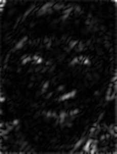
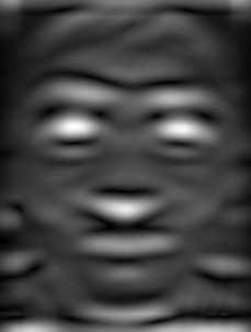
134 134 Figure 6.27: The impulse response of Gabor filter bank. From top to bottom, k = π 2, π 4, π 8 and from left to right θ = 0, π 4, π 2, 3π 4 Figure 6.28: The corresponding filtered results

135 135 Figure 6.29: Observation sequences for spatial HMMs The overlap between successive bands is specified by the variable constant S. Here the parameters W, L and S are set to be 114, 10 and 5, respectively. The observation is generated from top to bottom for each frame. The procedure is illustrated in Fig In order to reduce the high dimension of raw observation data, PCA is employed to find a set of eigenvectors accounting for the major variations of each observation band. The PCA coefficients from different Gabor channels are concatenated to form a compact representation for each observation band. The first order derivative of the observation is computed as the feature for recognition. For example, if 10 eigenvectors and 8 filter channels are used, the dimension of observation for each band is 80 = Experimental Results This subsection presents some experimental results based on Gabor filters and HHMMs. The Cohn-Kanade Action Unit AU-coded facial expression database [95] is used in the

136 136 experiments, that is designed to provide a valuable test-bed for the study of facial expression analysis. The public accessible portion of this database consists of 97 subjects with six prototype emotions: happiness, fear, surprise, anger, disgust, and sadness. Four basic classes, namely, happiness, fear, anger and sadness, are investigated in the experiment. The reason of this choice is that it is difficult for even humans to distinguish between fear and surprise and between anger and disgust subjectively. According to the facial action coding system FACS manual [80], we annotated and selected 32, 32, 20, and 28 sessions for each type of expression, respectively, because many sessions in this database contain only single AUs or AU combinations, that are incomplete expressions and inappropriate for expression analysis based on holistic faces. In addition, each expression session is performed by different subjects. Several experiments are carried out to evaluate the performance of the proposed approach for person-independent facial expression recognition in image sequences. The leave-one-out procedure [9] is adopted for training and testing due to the finite data size. In other words, for each class which has N sessions, N 1 sessions are used for training and the remaining session is used for testing. In total, N rounds of testing are available and the recognition rate is the average of the N recognition results. Four HHMMs as shown in Fig. 5.5 are built and trained for four types of emotions respectively, and the p.d.f of production states is modeled as Gaussian mixture models. The recognition of an observation sequence is achieved by computing its likelihood given each model and choosing the model with the maximum likelihood as the result.

137 137 Figure 6.30: Gabor responses to different expressions. From top to bottom: happiness, fear, anger and sadness First an experiment is conducted to compare the discriminating capability of different Gabor channels for different expressions. Table 6.5 lists the classification result for each channel and expression. From the statistics, we have some observations: 1 0 orientation has much less discriminating power for anger and sadness in all frequencies; 2 sadness is more sensitive to diagonal directions; 3 anger is sensitive to high frequency

138 138 Table 6.5: Classification results for individual Gabor channels index k θ Happiness32 Fear32 Anger20 Sadness28 π π π π π π π π π π π π π π π π components and vertical directions; 4 happiness and fear are more sensitive to low frequency components. In addition, table 6.6 compares the results with respect to different modulating frequencies. Clearly, high frequency components contain more discriminating information for facial expressions. Therefore, in tradeoff, we choose 9 Gabor channels 1,2,3,5,6,7,9,10,11 for following experiments. Fig shows the classification accuracy of different expressions with respect to the number of eigenvectors per channel. Here only the first four channels are investigated since they are the most discriminating channels for expression classification. As we can see, the average rate has little variance with the number of eigenvectors between 8 and 17. But it drops a lot beyond that range especially for expression anger. Furthermore, for

139 139 Table 6.6: Classification rate vs modulation frequency k Happiness32 Fear32 Anger20 Sadness28 π π π π Figure 6.31: Recognition rate vs number of eigenvectors per channel expression anger the best result is obtained with the number of eigenvectors between 8 and 10. In order to keep the observation vector in a reasonable size for the sake of reliable parameter estimation of HHMMs. 9 Gabor channels and 8 eigenvectors are chosen to form the observation vector with a dimension of 72. Table 6.7 is the confusion matrix for Gabor- HHMMs with 3 mixtures using 9 Gabor filters and 8 principle components.