Mediterranean Sea Production Centre MEDSEA_ANALYSIS_FORECAST_PHYS_006_013

Transcription

1 Mediterranean Sea Production Centre MEDSEA_ANALYSIS_FORECAST_PHYS_006_013 Contributors: E. Clementi, A. Grandi, P. Di Pietro, J. Pistoia, D. Delrosso, G. Mattia Approval date by the CMEMS product quality coordination team: 12/06/2018

2 CHANGE RECORD When the quality of the products changes, the QuID is updated and a row is added to this table. The third column specifies which sections or sub-sections have been updated. The fourth column should mention the version of the product to which the change applies. Issue Date Description of Change Author Validated By All Release of V3.2 version of the Med-Currents analysis and forecast product at 1/24 resolution All Release of V4version of the Med-Currents analysis and forecast product at 1/24 resolution E. Clementi, A. Grandi, P. DiPietro,, J. Pistoia, D. Delrosso, G. Mattia E. Clementi, A. Grandi, P. DiPietro,, J. Pistoia, D. Delrosso, G. Mattia Page 2/ 60

3 TABLE OF CONTENTS I Executive summary... 4 I.1 Products covered by this document... 4 I.2 Summary of the results... 4 I.3 Estimated Accuracy Numbers... 5 II Production system description II.1 Description of the Med-Currents V4 model system II.2 New features of the Med-Currents V4 system II.3 Upstream data and boundary condition of the NEMO-3DVAR system III Validation framework Validation results III.1 Temperature III.2 Seabed Temperature III.3 Salinity III.4 Sea Level Anomaly III.5 Sea Surface Height III.6 Currents III.7 Mixed Layer Depth IV System s Noticeable events, outages or changes V Quality changes since previous version VI References Page 3/ 60

4 I EXECUTIVE SUMMARY I.1 Products covered by this document The product covered by this document is the : the analysis and forecast nominal product of the physical component of the Mediterranean Sea with 1/24 (~4 km) horizontal resolution and 141 vertical levels. The variables produced are: 3D daily, hourly and monthly mean fields of: Potential Temperature, Salinity, Zonal and Meridional Velocity 2D daily, hourly and monthly mean fields of: Sea Surface Height, Mixed Layer Depth, Sea Bed Temperature (temperature of the deepest layer or level) I.2 Summary of the results The quality of the product, which is the analysis and forecast product of the CMEMS MED-Currents at CMEMS V4, is assessed over 1 year period from 01/01/2016 to 31/12/2016 by means of temperature, salinity, sea level anomaly, sea surface height, currents, seabed temperature and mixed layer depth using quasi-independent satellite and in-situ observations, independent (non-assimilated) coastal moorings, climatological datasets as well as the inter-comparison with the previous product corresponding to the CMEMS Med-Currents V3.2 version of the system. The main results of the quality assessment are summarized below: Sea Surface Height: the V4 system presents a similar accuracy in terms of sea surface height representation with respect to the previous version. The modeled sea surface height accuracy has been assessed using independent coastal tide-gauges, the error of the V4 system is about 4.62 cm in the considered period (year 2016). In addition, the quality of the predicted SLA has been assessed by considering the RMS of misfits between the model and the satellite along track observations. The new system presents an increased skill in terms of SLA if compared to V3.2 system for each of the available satellite decreasing the mean RMS difference of about 0.5 cm (from 4.3 to 3.9 cm considering the RMS misfit). The SLA increased quality in V4 system has been achieved by modifying the SLA data assimilation as specified in section II.2. Temperature: the temperature is accurate with an error below 0.85 o C when comparing to vertical insitu observations and below 0.7 o C when comparing SST to satellite observations. The accuracy of the temperature along the water column presents higher RMS differences at first layers, which decreases below 60m. Considering the SST, the RMS differences with respect to satellite observations varies according to the different areas of the basin ranging from 0.5 o C to 0.7 o C. The MED-Currents products usually have a cold bias in winter and a warm bias in summer. Med-Currents V3.2 and V4 systems exhibit similar skill in terms of surface temperature when comparing with satellite and coastal Page 4/ 60

5 moorings observations, while a slightly decrease in the surface temperature skill is shown when considering the RMS misfits, this can be caused by a lower number of assimilated data in the new system due to a modified pre-processing of insitu profiles. Salinity: the salinity is accurate with EAN RMS values lower than 0.18 PSU. The error is higher in the first layers and decreases significantly below 150 m. The V3.2 and V4 systems present very similar skill in predicting the salinity. Med-Currents V3.2 and V4 systems also exhibit similar skill in terms of surface salinity when comparing with coastal moorings observations. Currents: Surface currents RMS and bias are evaluated with respect to moored buoys in coastal areas and due to the low number of observations mainly located in coastal areas the statistical relevance of currents performance is poor. In addition to the surface currents validation assessment, some derived information on transport at Straits is included including the net, eastward and westward transport through the Strait of Gibraltar which are compared to literature values assessing that the new system (V4) transports values are slightly closer the ones provided by literature with respect to the previous system (V3.2). Moreover numerical geostrophic currents have been compared to the ones derived from satellite SLA gridded data in terms of daily basin averages showing a good ability of the model to represent the temporal variation of the satellite derived currents and kinetic energy. Bottom temperature: the bottom temperature of V4 system has been compared to SeaDataNet and WOA-V2 (World Ocean Atlas) monthly climatologies showing a good skill in representing the seasonal variability of the temperature at deepest level and a general overestimation with respect to the climatological dataset. The spatial pattern of the seabed temperature is correctly represented by the system. Mixed Layer Depth: the MLD predicted by V4 system has been compared to climatological values from literature (Houpert at al., 2015) showing that the model is able to correctly represent the depth of the mixed layer with differences in specific areas at different months. In general it can be noticed that the main differences can be due to the low resolution of the climatological dataset that moreover do not cover the whole domain of the Mediterranean Sea. I.3 Estimated Accuracy Numbers Estimated Accuracy Numbers (EANs), that are the mean and the RMS of the difference between the model and in-situ or satellite reference observations, are provided in the following table. EAN are computed for: Temperature; Salinity; Sea Surface Temperature (SST). Sea Level Anomaly (SLA) The observations used are: vertical profiles of temperature and salinity from Argo, XBTs and Gliders floats: INSITU_GLO_NRT_OBSERVATIONS_013_030, INSITU_MED_TS_NRT_OBSERVATIONS_013_035 Page 5/ 60

6 SST satellite data from Copernicus OSI-TAC product: SST_MED_SST_L4_NRT_OBSERVATIONS_010_004 Satellite Sea Level along track data from Copernicus SL-TAC product: SEALEVEL_MED_SLA_L3_NRT_OBSERVATIONS_008_019 SEALEVEL_MED_SLA_ASSIM_L3_NRT_OBSERVATIONS_008_021 The EANs are evaluated for the V3.2 and V4 systems over 1 year period from January to December 2016 and are computed over 9 vertical layers (for temperature and salinity) and for the Mediterranean Sea and 16 sub-regions Figure 1: (1) Alboran Sea, (2) South West Med 1 (western part), (4) South West Med 2 (eastern part), (3) North West Med, (6) Tyrrhenian Sea 1 (northern part), (5) Tyrrhenian Sea 2 (southern part), (11) Adriatic Sea 1 (northern part), (10) Adriatic Sea 2 (southern part), (7) Ionian Sea 1 (western part), (9) Ionian Sea 2 (north-eastern part), (8) Ionian Sea 2 (south-eastern part), (13) Aegean Sea, (12) Levantine Sea 1 (western part), (14) Levantine Sea 2 (central-northern part), (15) Levantine Sea 3 (central southern part), (16) Levantine Sea 4 (eastern part). Figure 1. The Mediterranean Sea sub-regions subdivision for validation metrics Moreover, the EANs of temperature and salinity are then evaluated at 9 different layers: 0-10, 10-30, 30-60, , , , , , [m] in order to better verify the model ability to represent the vertical structure of the temperature and salinity fields. Page 6/ 60

7 T prod - T ref [ o C] Layer (m) Mean T-<X-Y>m-D-CLASS4-PROF-BIAS- Jan2016-Dec2016 V4 system RMSD T-<X-Y>m-D-CLASS4-PROF-RMSD- Jan2016-Dec Table 1: EANs of temperature at different vertical layers evaluated for V4 system for the year 2016: T-<X-Y>m-D- CLASS4-PROF-BIAS-Jan2016-Dec2016, T-<X-Y>m-D-CLASS4-PROF-RMSD-Jan2016-Dec2016 specified in Table 9 SST prod SST ref [ o C] V4 system REGION Mean SST-D-CLASS4-RAD-BIAS-Jan2016-Dec2016 RMSD SST-D-CLASS4-RAD-RMSD-Jan2016-Dec2016 MED SEA REGION REGION REGION REGION REGION REGION REGION REGION REGION REGION REGION REGION REGION REGION REGION REGION Table 2: EANs of Sea Surface Temperature evaluated for V4 system for the year 2016 for the Mediterranean Sea and 16 regions (see Figure 1): SST-D-CLASS4-RAD-BIAS-Jan2016-Dec2016, SST-D-CLASS4-RAD-RMSD-Jan2016- Dec2016 specified in Table 9. Page 7/ 60

8 S prod S ref [PSU] Layer (m) Mean S-<X-Y>m-D- CLASS4-PROF- BIAS-Jan2016- Dec2016 V4 system RMSD S-<X-Y>m-D- CLASS4-PROF- RMSD-Jan2016- Dec Table 3: EANs of salinity at different vertical layers evaluated for V4 system for year 2016: S-<X-Y>m-D-CLASS4- PROF-BIAS-Jan2016-Dec 2016, S-<X-Y>m-D-CLASS4-PROF-RMSD-Jan2016-Dec 2016 specified in Table 9 SLA prod SLA ref [cm] REGION V3.2 system V4 system RMSD SLA-D-CLASS4-ALT-RMSD-Jan2016- Dec2016 RMSD SLA-D-CLASS4-ALT-RMSD-Jan2016- Dec2016 MED SEA REGION REGION REGION REGION REGION REGION REGION REGION REGION REGION REGION 11 NA NA REGION REGION REGION REGION REGION Table 4: EANs of Sea Level evaluated for V3.2 and V4 systems for year 2016 for the Mediterranean Sea and 16 regions (see Figure 1): SLA-D-CLASS4-ALT-RMSD-Jan2016-Dec 2016 see Table 9 Page 8/ 60

9 The metrics of Table 1 and Table 2 give indications about the accuracy of temperature variable along the water column and at the surface for the Mediterranean Sea and 16 sub-regions. The values for all the vertical levels are computed using Argo profiles while the SST is evaluated by comparing with satellite observations. The temperature RMS and MEAN values are higher at the first levels and decrease significantly below the fourth layer. The error is always lower than 0.85 o C along the water column, while it ranges between 0.47 and 0.72 o C considering the SST. The statistics listed in S prod S ref [PSU] Layer (m) Mean S-<X-Y>m-D- CLASS4-PROF- BIAS-Jan2016- Dec2016 V4 system RMSD S-<X-Y>m-D- CLASS4-PROF- RMSD-Jan2016- Dec Table 3 give indications about the accuracy of the salinity product. The values for all the levels are computed using Argo profiles. The skill of the system presents a RMS difference always lower than 0.2 PSU with higher error at surface that decreases below 150m. The metrics shown in Table 4 define the accuracy of sea level anomaly. The statistics are computed along the satellite tracks. In this case a comparison with the previous system (V3.2) is provided in order to show the improvements achieved with the modified SLA data assimilation. The new system presents in almost all regions an increased skill with an averaged reduction of the RMS difference of about 0.3 cm with respect to the previous system. One of the regions presents no data since the new SLA data assimilation scheme (using the dynamic height) prevents the assimilation of data in areas shallower than 1000 m. Page 9/ 60

10 II PRODUCTION SYSTEM DESCRIPTION Production centre name: INGV Production system name: Analysis and Forecast Med-Currents system at CMEMS V4 CMEMS Product name: External product: Temperature (3D), Salinity (3D), Meridional and Zonal Currents (3D), Sea Surface Height (2D), Mixed Layer Depth (2D), Seabed Temperature (2D) Frequency of model output: daily (24-hrs) averages, hourly (1-hr) averages, monthly averages Geographical coverage: W E; N N (Gulf of Biscay is excluded) Horizontal resolution: 1/24 Vertical coverage: From surface to 5754m (141 vertical unevenly spaced levels). Length of forecast: 10 days for the daily mean fields, 5 days for the hourly mean fields. Frequency of forecast release: Daily. Analyses: Yes. Hindcast: Yes. Frequency of analysis release: Weekly on Tuesday. Frequency of hindcast release: Daily. The Analyses and forecasts physical product of the Med-MFC is produced with two different cycles. The analysis cycle is done weekly, on Tuesday, for the previous 15 days, because a shorter analysis cycle would not allow getting enough observations into the assimilation, for both in situ and satellite data. The forecast cycle is daily and it produces 10-day forecast fields starting each day at 12:00:00 UTC. The forecast is initialized by a background field every day except Tuesday, when an analysis is used. The production chain is illustrated in Figure 2. Page 10/ 60

11 Figure 2. Scheme of the analysis and forecast CMEMS Med-Currents processing chain. The Med-Currents system run is composed by several steps: 1. Upstream Data Acquisition, Pre-Processing and Control of: ECMWF atmospheric forcing (Numerical Weather Prediction), Satellite (SLA and SST) and in-situ (T and S) data. 2. Forecast/Hindcast: NEMO code is run to produce one day of hindcast and 10-day forecast. 3. Analysis/Hindcast (only on Tuesday): NEMO code is combined with a 3DVAR assimilation scheme in order to produce the best estimation of the sea (i.e. analysis). The NEMO+3DVar system is running for 15 days into the past in order to use the best available along tack SLA products. The latest day of the 15 days of analyses, produces the initial condition for the 10- day forecast. 4. Post processing: the model output is processed in order to obtain the products for the CMEMS catalogue. 5. Output Delivery. II.1 Description of the Med-Currents V4 model system The Mediterranean Forecasting System, MFS, (Pinardi et al., 2003, Pinardi and Coppini 2010, Tonani et al., 2014) is providing, since year 2000, analysis and short-term forecast of the main physical parameters in the Mediterranean Sea and it is the physical component of the Med-MFC called Med- Currents. The analysis and forecast Med-Currents system at CMEMS V4 is provided by means of a coupled hydrodynamic-wave model implemented over the whole Mediterranean basin and extended into the Atlantic Sea in order to better resolve the exchanges with the Atlantic Ocean at the Strait of Gibraltar. The model horizontal grid resolution is 1/24 (ca. 4 km) and has 141 unevenly spaced vertical levels. Page 11/ 60

12 The hydrodynamics are supplied by the Nucleous for European Modelling of the Ocean (NEMO v3.6) while the wave component is provided by WaveWatch-III. The model solutions are corrected by the variational assimilation (based on a 3DVAR scheme) of temperature and salinity vertical profiles and along track satellite Sea Level Anomaly observations. Circulation model component (NEMO) The oceanic equations of motion of Med-currents system are solved by an Ocean General Circulation Model (OGCM) based on NEMO (Nucleus for European Modelling of the Ocean) version 3.6 (Madec et al., 2016). The code is developed and maintained by the NEMO-consortium. NEMO has been implemented in the Mediterranean at 1/24 x 1/24 horizontal resolution and 141 unevenly spaced vertical levels (Clementi et al., 2017a) with time step of 300sec. The model covers the whole Mediterranean Sea and also extends into the Atlantic in order to better resolve the exchanges with the Atlantic Ocean at the Strait of Gibraltar. The NEMO code solves the primitive equations using the time-splitting technique that is the external gravity waves are explicitly resolved with non-linear free surface formulation and time-varying vertical z-star coordinates. The advection scheme for active tracers, temperature and salinity, is a mixed up-stream/muscl (Monotonic Upwind Scheme for Conservation Laws, Van Leer 1979), originally implemented by Estubier and Le vy (2000) and modified by Oddo et al. (2009). The vertical diffusion and viscosity terms are a function of the Richardson number as parameterized by Pacanowsky and Philander (1981). The model interactively computes air-surface fluxes of momentum, mass, and heat. The bulk formulae implemented are described in Pettenuzzo et al. (2010) and are currently used in the Mediterranean operational system (Tonani et al. 2015). A detailed description of other specific features of the model implementation can be found in Oddo et al. (2009, 2014). The vertical background viscosity and diffusivity values are set to 1.2e-6 [m2/s] and 1.0e-7 [m2/s] respectively, while the horizontal bilaplacian eddy diffusivity and viscosity are set respectively equal to -1.2e8 [m4/s] and -2.e8 [m4/s]. A quadratic bottom drag coefficient with a logarithmic formulation has been used according to Maraldi et al. (2013) and the model uses vertical partial cells to fit the bottom depth shape. The hydrodynamic model is nested in the Atlantic within the Global analysis and forecast system GLO- MFC daily data set (1/12 horizontal resolution, 50 vertical levels) that is interpolated onto the Med- Currents model grid. Details on the nesting technique and major impacts on the model results are in Oddo et al., The model is forced by momentum, water and heat fluxes interactively computed by bulk formulae using the 6-hours (for the first 3 days of forecast a 3-hours temporal resolution is used), 1/8 horizontal-resolution operational analysis and forecast fields from the European Centre for Medium- Range Weather Forecasts (ECMWF) and the model predicted surface temperatures (details of the airsea physics are in Tonani et al., 2008). The water balance is computed as Evaporation minus Precipitation and Runoff. The evaporation is derived from the latent heat flux, precipitation is provided by ECMWF as daily averages, while the runoff of the 39 rivers implemented is provided by monthly mean datasets: the Global Runoff Data Centre dataset (Fekete et al., 1999) for the Po, Ebro, Nile and Rhone rivers; the dataset from Raicich (1996) for: Vjosë, Seman rivers; the UNEP-MAP dataset (Implications of Climate Change for the Albanian Coast, Mediterranean Action Plan, MAP Technical Page 12/ 60

13 Reports Series No.98., 1996) for the Buna/Bojana river; the PERSEUS dataset for the following 32 rivers: Piave, Tagliamento, Soca/Isonzo, Livenza, Brenta-Bacchiglione, Adige, Lika, Reno, Krka, Arno, Nerveta, Aude, Trebisjnica, Tevere/Tiber, Mati, Volturno, Shkumbini, Struma/Strymonas, Meric/Evros/Maritsa, Axios/Vadar, Arachtos, Pinios, Acheloos, Gediz, Buyuk Menderes, Kopru, Manavgat, Seyhan, Ceyhan, Gosku, Medjerda, Asi/Orontes. The Dardanelles Strait is closed but considered as volume input (Kourafalou and Barbopoulos, 2003) through a river-like parameterization. The topography is created starting from the GEBCO 30arc-second grid ( filtered (using a Shapiro filter) and manually modified in critical areas such as: islands along the Eastern Adriatic coasts, Gibraltar and Messina straits, Atlantic box edge. Wave model component (WW3) The Wave dynamic is solved by a Mediterranean implementation of the WaveWatch-III code version 3.14 (Tolman 2009). WaveWatch covers the same domain and follows the same horizontal discretization of the circulation model (1/24 x 1/24 ) with a time step of 300 sec. The wave model uses 24 directional bins (15 directional resolution) and 30 frequency bins (ranging between 0.05Hz and Hz) to represent the wave spectral distribution. WW3 has been forced by the same 1/8 horizontal resolution ECMWF atmospheric forcings (the same used to force the hydrodynamic model). The wind speed is then modified by considering a stability parameter depending on the air-sea temperature difference according to Tolman The wave model takes into consideration the surface currents for wave refraction but assumes no interactions with the ocean bottom. WW3 model solves the wave action balance equation that describes the evolution, in slowly varying depth domain and currents, of a 2D ocean wave spectrum where individual spectral component satisfies locally the linear wave theory. In the present application WW3 has been implemented following WAM cycle4 model physics (Gunther et al. 1993). Wind input and dissipation terms are based on Janssen s quasi-linear theory of wind-wave generation (Janssen, 1989, 1991). The dissipation term is based on Hasselmann (1974) whitecapping theory according to Komen et al. (1984). The non-linear wave-wave interaction is modelled using the Discrete Interaction Approximation (DIA, Hasselmann et al., 1985). No interactions with the ocean bottom are considered. Model coupling (NEMO-WW3) The coupling between the hydrodynamic model (NEMO) and the wave model (WW3) is achieved by an online hourly two-way coupling and consists in exchanging the following fields: NEMO sends to WW3 the air-sea temperature difference and the surface currents, while WW3 sends to NEMO the neutral drag coefficient used to evaluate the surface wind stress. More details on the model coupling and on the impact of coupled system on both wave and circulation fields can be found in Clementi et al. (2017b). Page 13/ 60

14 Data Assimilation scheme The data assimilation system is the 3DVAR scheme developed by Dobricic and Pinardi (2008) and modified by Storto et al. (2015). The background error correlation matrices vary monthly for each grid point in the discretized domain of the Mediterranean Sea. Observational error covariance matrix is evaluated with Desroziers et al. (2005) relationship. EOFs have been evaluated from a three years simulation run (in the future a new set of EOFs will be evaluated from an analysis run). The assimilated data include: along track Sea Level Anomaly (a satellite product accounting for atmospheric pressure effect is used) from CLS SL-TAC, and in-situ vertical temperature and salinity profiles from VOS XBTs (Voluntary Observing Ship-eXpandable Bathythermograph) and ARGO floats. Objective Analyses-Sea Surface Temperature (OA-SST) fields from CNR-ISA OSI-TAC are used for the correction of surface heat fluxes with the relaxation constant of 40 W m -2 K -1. II.2 New features of the Med-Currents V4 system The new features of the analysis and forecast Med-Currents V4 product with respect to the previous version (V3.2) are mainly due to the modified data assimilation scheme for the SLA in order to improve the SLA skill from the previous system and the re-introduction of the online coupling between NEMO and WW3. The main differences between the CMEMS Med-Currents V3.2 and V4 systems are summarized in. Initaial Conditions Data Assimilation Wave coupling Table 5 and described hereafter. CMEMS Med-Currents V3.2 WOA-V2 Winter Clim T/S (1/1/2013) 3DVAR Storto et al. (2015) SLA: barotropic model No CMEMS Med-Currents V4 WOA-V2 Winter Clim T/S (1/1/2015) 3DVAR Storto et al. (2015) SLA: dynamic height Yes (through Surface Drag Coeff.) Initaial Conditions Data Assimilation CMEMS Med-Currents V3.2 WOA-V2 Winter Clim T/S (1/1/2013) 3DVAR Storto et al. (2015) SLA: barotropic model CMEMS Med-Currents V4 WOA-V2 Winter Clim T/S (1/1/2015) 3DVAR Storto et al. (2015) SLA: dynamic height Page 14/ 60

15 Wave coupling No Yes (through Surface Drag Coeff.) Table 5: Differences between CMEMS Med-Currents V3.2 and V4 systems. 1. Modified SLA data assimilation The main difference between CMEMS V3.2 and CMEMS V4 data assimilation scheme is related to the SLA operator, which has been moved from the barotropic model to the dynamic height balance. This change has been included in order to solve a slow down of the convergence in the cost function in the case of the barotropic model which caused a decrease in the SLA skill in the CMEMS V3.2 system. The use of the Dynamic height allows a faster cost function convergence and, even if it discards all the observation in areas shallower than 1000m, it provides an enhanced skill of the SLA in the new V4 system. 2. Coupling with wave model The coupling between NEMO and the wave model WW3, that was not included in the previous system (V3.2) due to technical issues caused by the increased resolution (from 1/16 to 1/24 horizontal resolution), is now provided in the new system (V4). The coupling mechanism is the same as the one included in the previous version at 1/16 resolution but with decreased wave model time step which is now of 300 sec (instead of 600 sec). More details on the coupling mechanism and on the effects on the circulation fields are provided in Clementi et al. (2017b). II.3 Upstream data and boundary condition of the NEMO-3DVAR system The CMEMS MED-Currents system uses the following upstream data: 1. Atmospheric forcing (including precipitation): NWP 6-h (3-h for the first 3 days of forecast), horizontal-resolution operational analysis and forecast fields from the European Centre for Medium-Range Weather Forecasts (ECMWF) distributed by the Italian National Meteo Service (USAM/CNMA) 2. Runoff: Global Runoff Data Centre dataset (Fekete et al., 1999) for Po, Ebro, Nile and Rhone, the dataset from Raicich (Raicich, 1996) for the Adriatic rivers Vjosë and Seman; the UNEP- MAP dataset (Implications of Climate Change for the Albanian Coast, Mediterranean Action Plan, MAP Technical Reports Series No.98., 1996) for the Buna/Bojana river; the PERSEUS project dataset for the new 32 rivers added. 3. Data assimilation: o o Temperature and Salinity vertical profiles from Copernicus INSITU TAC INSITU_MED_NRT_OBSERVATIONS_013_035 INSITU_GLO_NRT_OBSERVATIONS_013_030 Satellite along track Sea Level Anomaly from Copernicus SL TAC: Page 15/ 60

16 o SEALEVEL_MED_SLA_ASSIM_L3_NRT_OBSERVATIONS_008_021 (till 31 th May 2017) SEALEVEL_MED_SLA_L3_NRT_OBSERVATIONS_008_019 (till 31 th May 2017) SEALEVEL_MED_PHY_ASSIM_L3_NRT_OBSERVATIONS_008_048 (from 1 st June 2017). Satellite SST from Copernicus OSI TAC (nudging): SST_MED_SST_L4_NRT_OBSERVATIONS_010_ Initial conditions of temperature and salinity at 1/1/2013 are the winter climatological fields from WOA13 V2 (World Ocean Atlas 2013 V2, 5. Lateral boundary conditions from Copernicus Global Analysis and Forecast system: GLOBAL_ANALYSIS_FORECAST_PHY_001_024 at 1/12 horizontal resolution, 50 vertical levels. In particular for the lateral boundary condition the following conditions are considered: 1. The radiative phase velocity (Cx and Cy) is computed at the open boundaries using Orlanski (NPO) formulation with adaptative nudging for baroclinic velocities and tracers (Marchesiello et al., 2001). 2. The radiation algorithm is applied to zonal and meridional components of the open boundary conditions velocities using the phase velocities computed at point 1 3. The Flather boundary condition (Flather, 1976) is applied to barotropic velocities at open boundaries for the time-splitting free surface case 4. The total velocities are updated on the basis of point 2 and 3 5. For tracers the 2D radiation condition is applied using radiative phase velocity computed at point 1 Page 16/ 60

17 III VALIDATION FRAMEWORK In order to evaluate and assure the quality of the product, an assimilation experiment has been performed using the system described in section II, that is going to be operational starting in April 2018, and covering 3 years from January 2015 to December 2017 (the period from January to December 2015 is considered as a spin-up time). In particular the qualification task has been carried out over 1 year period, from January to December 2016, based on Class 1, 2 and 4 diagnostics. The performance of the Med-Currents V4 system has been assessed by using external products, i.e. temperature, salinity, sea level anomaly using quasi-independent satellite and in-situ observations, moreover independent moorings are used to assess the model (temperature, salinity, sea level and currents) skill through an independent dataset in compliance with the Scientific PreOperational Qualification Plan (ScQP) and climatological datasets have been used to assess the quality of the seabed temperature and mixed layer depth. Quasi-independent data are all the observations (Satellite SLA and SST and in situ vertical profiles of temperature and salinity from XBT, Argo and Glider) that are assimilated into the system. Diagnostic in terms of RMS of the misfits and/or bias are computed. The independent in-situ observations are delivered by a network of 13 institutes from Copernicus INSITU TAC (Puertos del Estado, IFREMER, CNR-IAMC-ISSIA-ISMAR, HCMR, OC-UCY, CSIC, OGS, ISPRA, NIB-MBS) and MonGOOS partners (IOLR, UMT-IOI-POU, IASA-UAT, IMS-METU) and are downloaded operationally on a daily basis by the Med- MFC operational centre at INGV. The datasets of observations used for the qualification task are listed below: in Table 6 and in Table 7 there are respectively the lists of the used quasi-independent and independent data with the corresponding CMEMS product names. In INDEPENDENT DATA VARIABLE AVAILABILITY in 2016 TEMPERATURE 15 SALINITY 7 SEA LEVEL 49 CURRENTS 8 SST 18 Table 8 there are the numbers of all the available independent moored buoys, for the year 2016, and Figure 3 shows the locations of moored buoys. QUASI-INDEPENDENT DATA Page 17/ 60

18 TYPE ARGO, XBT CTD, GLIDER CMEMS PRODUCT NAME INSITU_GLO_NRT_OBSERVATIONS_013_030 INSITU_MED_NRT_OBSERVATIONS_013_035 SLA SST SEALEVEL_MED_SLA_ASSIM_L3_NRT_OBSERVATIONS_008_021 (till 31th May 2017) SEALEVEL_MED_SLA_L3_NRT_OBSERVATIONS_008_019 (till 31th May 2017) SEALEVEL_MED_PHY_ASSIM_L3_NRT_OBSERVATIONS_008_048 (from 1st June 2017) SST_MED_SST_L4_NRT_OBSERVATIONS_010_004_a Table 6: list of the quasi-independent observations INDEPENDENT DATA TYPE MOORED BUOYS CMEMS PRODUCT NAME INSITU_MED_NRT_OBSERVATIONS_013_035 Table 7: list of the independent observations INDEPENDENT DATA VARIABLE AVAILABILITY in 2016 TEMPERATURE 15 SALINITY 7 SEA LEVEL 49 CURRENTS 8 SST 18 Table 8: Availability of the independent data (moored buoy) during 2016 Page 18/ 60

19 Figure 3: Locations of moored independent in-situ data in the Mediterranean Sea. The list of metrics used to provide an overall assessment of the product, to quantify the differences with the available observations and to assess the improvements with respect to the previous system (CMEMS V3.2) is presented in Table 9 in accordance to the Scientific PreOperational Qualification Plan. Page 19/ 60

20 Name Description Ocean parameter Supporting reference dataset Quantity NRT evaluation of Med-MFC-Currents using semi-independent data: Estimate Accuracy Numbers T-<X-Y>m-D-CLASS4- PROF-RMSD-Jan2016- Dec2016 Temperature vertical profiles comparison with Copernicus INSITU TAC data at 9 layers for the Mediterranean basin. Temperature Argo floats from the Copernicus INSITU TAC products: INSITU_GLO_NRT_OBSERVATIONS_013_030 INSITU_MED_NRT_OBSERVATIONS_013_035 Temperature daily RMSs of the difference between model and insitu observations averaged over the qualification testing period (Jan-Dec 2016). This quantity is evaluated on the model analysis. The statistics are defined for all the Mediterranean Sea and are evaluated for 9 different layers (0-10, 10-30, 30-60, , , , , , m) T-<X-Y>m-D-CLASS4- PROF-BIAS-Jan2016- Dec2016 Temperature vertical profiles comparison with Copernicus INSITU TAC data at 9 layers for the Mediterranean basin. Temperature Argo floats from the Copernicus INSITU TAC products: INSITU_GLO_NRT_OBSERVATIONS_013_030 INSITU_MED_NRT_OBSERVATIONS_013_035 Temperature daily mean differences between model and insitu observations averaged over the qualification testing period (Jan- Dec 2016). This quantity is evaluated on the model analysis. The statistics are defined for all the Mediterranean Sea and are evaluated for 9 different layers (0-10, 10-30, 30-60, , , , , , m) S-<X-Y>m-D-CLASS4- PROF-RMSD-Jan2016- Dec2016 Salinity vertical profiles comparison with Copernicus INSITU TAC data at 9 layers for the Mediterranean basin. Salinity Argo floats from the Copernicus INSITU TAC products: INSITU_GLO_NRT_OBSERVATIONS_013_030 INSITU_MED_NRT_OBSERVATIONS_013_035 Salinity daily RMSs of the difference between model and insitu observations averaged over the qualification testing period (Jan- Dec 2016). This quantity is evaluated on the model analysis. The statistics are defined for all the Mediterranean Sea and are evaluated for 9 different layers (0-10, 10-30, 30-60, , , , , , m) Page 20/ 60

21 S-<X-Y>m-D-CLASS4- PROF-BIAS-Jan2016- Dec2016 Salinity vertical profiles comparison with Copernicus INSITU TAC data at 9 layers for the Mediterranean basin. Salinity Argo floats from the Copernicus INSITU TAC products: INSITU_GLO_NRT_OBSERVATIONS_013_030 INSITU_MED_NRT_OBSERVATIONS_013_035 Salinity daily mean differences between model and insitu observations averaged over the qualification testing period (Jan- Dec 2016). This quantity is evaluated on the model analysis. The statistics are defined for all the Mediterranean Sea and are evaluated for 9 different layers (0-10, 10-30, 30-60, , , , , , m) SLA-D-CLASS4-ALT- RMSD-Jan2016- Dec2016 Sea level anomaly comparison with Copernicus Sea Level TAC (satellite along track) data for the Mediterranean basin and selected subbasins. Sea Anomaly Level Satellite Sea Level along track data from Copernicus Sea Level TAC product: SEALEVEL_MED_SLA_L3_NRT_OBSERVATIONS_ 008_019 SEALEVEL_MED_SLA_ASSIM_L3_NRT_OBSERV ATIONS_008_021 Sea level daily RMSs of the difference between model and satellite observations averaged over the qualification testing period (Jan-Dec 2016). This quantity is evaluated on the model analysis. The statistics are defined for all the Mediterranean Sea and 16 selected sub-basins. SST-D-CLASS4-RAD- RMSD-Jan2016- Dec2016 Sea Surface Temperature comparison with SST Copernicus OSI TAC L4 (satellite) data for the Mediterranean basin and selected subbasins. Sea Surface Temperature SST satellite data from Copernicus OSI TAC L4 product: SST_MED_SST_L4_NRT_OBSERVATIONS_010_0 04 Sea surface temperature daily RMSs of the difference between model and satellite observations averaged over the qualification testing period (Jan-Dec 2016). This quantity is evaluated on the model analysis. The statistics are defined for all the Mediterranean Sea and 16 selected sub-basins. SST-D-CLASS4-RAD- BIAS-Jan2016-Dec2016 Sea Surface Temperature comparison with SST Copernicus OSI TAC L4 (satellite) data for the Mediterranean basin and selected subbasins. Sea Surface Temperature SST satellite data from Copernicus OSI TAC L4 product: SST_MED_SST_L4_NRT_OBSERVATIONS_010_0 04 Sea surface temperature daily mean differences between model and satellite observations averaged over the qualification testing period (Jan-Dec 2016). This quantity is evaluated on the model analysis. The statistics are defined for all the Mediterranean Sea and 16 selected sub-basins. Page 21/ 60

22 NRT evaluation of Med-MFC-Currents using semi-independent data. Daily comparison T-<X-Y>m-D-CLASS4- PROF-RMSD-Jan2016- Dec2016 Temperature vertical profiles comparison with Copernicus INSITU TAC data at 9 layers for the Mediterranean basin Temperature Argo floats from the Copernicus INSITU TAC products: INSITU_GLO_NRT_OBSERVATIONS_013_030 INSITU_MED_NRT_OBSERVATIONS_013_035 Time series of temperature daily RMSs of the difference between model and insitu observations evaluated over the qualification testing period (2016). This quantity is evaluated on the model analysis. The statistics are defined for all the Mediterranean Sea and are evaluated for seven different layers (0-10, 10-30, 30-60, , , , , , m) S-<X-Y>m-D-CLASS4- PROF-RMSD-Jan2016- Dec2016 Salinity vertical profiles comparison with Copernicus INSITU TAC data at 9 layers for the Mediterranean basin Salinity Argo floats from the Copernicus INSITU TAC products: INSITU_GLO_NRT_OBSERVATIONS_013_030 INSITU_MED_NRT_OBSERVATIONS_013_035 Time series of salinity daily RMSs of the difference between model and insitu observations evaluated over the qualification testing period (2016). This quantity is evaluated on the model analysis. The statistics are defined for all the Mediterranean Sea and are evaluated for seven different layers (0-10, 10-30, 30-60, , , , , , m) SLA-D-CLASS4-ALT- RMSD-Jan2016- Dec2016 Sea level anomaly comparison with Copernicus Sea Level TAC (satellite along track) data for the Mediterranean basin Sea Anomaly Level Satellite Sea Level along track data from Copernicus Sea Level TAC product: SEALEVEL_MED_SLA_L3_NRT_OBSERVATIONS_ 008_019 SEALEVEL_MED_SLA_ASSIM_L3_NRT_OBSERV ATIONS_008_021 Time series of sea level anomaly daily RMSs of the difference between model and satellite observations evaluated over the qualification testing period (2016). This quantity is evaluated on the model analysis. The statistics are defined for all the Mediterranean Sea. SST-D-CLASS4-RAD- RMSD-Jan2016- Dec2016 Sea Surface Temperature comparison with SST Copernicus OSI TAC L4 (satellite) data for the Mediterranean basin Sea Surface Temperature SST satellite data from Copernicus OSI TAC L4 product: SST_MED_SST_L4_NRT_OBSERVATIONS_010_0 04 Time series of sea surface temperature daily RMSs of the difference between model and satellite observations evaluated over the qualification testing period (2016). This quantity is evaluated on the model analysis. The statistics are defined for all the Mediterranean Sea. Page 22/ 60

23 SST-D-CLASS4-RAD- BIAS-Jan2016-Dec2016 Sea Surface Temperature comparison with SST Copernicus OSI TAC L4 (satellite) data for the Mediterranean basin Sea Surface Temperature SST satellite data from Copernicus OSI TAC L4 product: SST_MED_SST_L4_NRT_OBSERVATIONS_010_0 04 Time series of sea surface temperature daily BIAS (difference between model and satellite observations) evaluated over the qualification testing period (2016). This quantity is evaluated on the model analysis. The statistics are defined for all the Mediterranean Sea. NRT evaluation of Med-MFC-Currents using semi-independent data. Weekly comparison of misfits T-<X-Y>m-W-CLASS4 PROF-RMSD-MED- Jan2016-Dec 2016 Temperature vertical profiles comparison with assimilated Copernicus INSITU TAC data at 5 specified depths. Temperature Argo floats, Gliders and XBT from the Copernicus INSITU TAC products: INSITU_GLO_NRT_OBSERVATIONS_013_030 INSITU_MED_NRT_OBSERVATIONS_013_035 Time series of weekly RMSs of temperature misfits (observation minus model value transformed at the observation location and time). Together with the time series, the average value of weekly RMSs is evaluated over the qualification testing period (2016). This quantity is evaluated on the model analysis. The statistics are defined for all the Mediterranean Sea and are evaluated at five different depths: 8, 30, 150, 300 and 600 m. S-<X-Y>m-W-CLASS4 PROF-RMSD-MED- Jan2016-Dec 2016 Salinity vertical profiles comparison with assimilated Copernicus INSITU TAC data at 5 specified depths. Salinity Argo floats from the Copernicus INSITU TAC products: INSITU_GLO_NRT_OBSERVATIONS_013_030 INSITU_MED_NRT_OBSERVATIONS_013_035 Time series of weekly RMSs of salinity misfits (observation minus model value transformed at the observation location and time). Together with the time series, the average value of weekly RMSs is evaluated over the qualification testing period (2016). This quantity is evaluated on the model analysis. The statistics are defined for all the Mediterranean Sea and are evaluated at five different depths: 8, 30, 150, 300 and 600 m. Page 23/ 60

24 SLA-SURF-W-CLASS4- ALT-RMSD-MED- Jan2016-Dec 2016 Sea level anomaly comparison with assimilated Copernicus Sea Level TAC satellite along track data for the Mediterranean basin. Sea Anomlay Level Satellites (Jason2, Jason2N, Jason3, CryoSat-2, Saral/Altika) Sea Level along track data from Copernicus Sea Level TAC products: SEALEVEL_MED_SLA_L3_NRT_OBSERVATIONS_ 008_019 SEALEVEL_MED_SLA_ASSIM_L3_NRT_OBSERV ATIONS_008_021 Time series of weekly RMSs of sea level anomaly misfits (observation minus model value transformed at the observation location and time). Together with the time series, the average value of weekly RMSs is evaluated over the qualification testing period (2016). This quantity is evaluated on the model analysis. The statistics are defined for all the Mediterranean Sea and are evaluated for the different assimilated satellites. NRT evaluation of Med-MFC-Currents using independent data. Daily comparison with moored buoys T-SURF-D-CLASS2- MOOR-RMSD-Jan2016- Dec2016 Temperature comparison with Copernicus INSITU TAC and MonGOOS data. Temperatue Moored buoys from Copernicus InSitu TAC products: INSITU_GLO_NRT_OBSERVATIONS_013_030 INSITU_MED_NRT_OBSERVATIONS_013_035 Moored buoys from MonGOOS partners Time series of daily temperature of insitu observations and model outputs evaluated for the surface layer (0-3 m) over the qualification testing period. Together with the time series, the average value of daily RMSs is evaluated over the qualification testing period. This quantity is evaluated on the model analysis. T-SURF-D-CLASS2- MOOR-BIAS-Jan2016- Dec2016 Temperature comparison with Copernicus INSITU TAC and MonGOOS data. Temperatue Moored buoys from Copernicus InSitu TAC products: INSITU_GLO_NRT_OBSERVATIONS_013_030 INSITU_MED_NRT_OBSERVATIONS_013_035 Moored buoys from MonGOOS partners Time series of daily temperature of insitu observations and model outputs evaluated for the surface layer (0-3 m) over the qualification testing period. Together with the time series, the average value of daily bias is evaluated over the qualification testing period. This quantity is evaluated on the model analysis. S-SURF-D-CLASS2- MOOR-RMSD-Jan2016- Dec2016 Salinity comparison with Copernicus INSITU TAC and MonGOOS data. Salinity Moored buoys from Copernicus InSitu TAC products: INSITU_GLO_NRT_OBSERVATIONS_013_030 INSITU_MED_NRT_OBSERVATIONS_013_035 Moored buoys from MonGOOS partners Time series of daily salinity of insitu observations and model outputs evaluated for the surface layer (0-3 m) over the qualification testing period. Together with the time series, the average value of daily RMSs is evaluated over the qualification testing period. This quantity is evaluated on the model analysis. Page 24/ 60

25 S-SURF-D-CLASS2- MOOR-BIAS-Jan2016- Dec2016 Salinity comparison with Copernicus INSITU TAC and MonGOOS data. Salinity Moored buoys from Copernicus InSitu TAC products: INSITU_GLO_NRT_OBSERVATIONS_013_030 INSITU_MED_NRT_OBSERVATIONS_013_035 Moored buoys from MonGOOS partners Time series of daily salinity of insitu observations and model outputs evaluated for the surface layer (0-3 m) over the qualification testing period. Together with the time series, the average value of daily bias is evaluated over the qualification testing period. This quantity is evaluated on the model analysis. SL-SURF-D-CLASS2-TG- RMSD-Jan2016- Dec2016 Sea Level comparison with Copernicus INSITU TAC and MonGOOS data. Sea Level Tide-gauges from Copernicus InSitu TAC products: INSITU_GLO_NRT_OBSERVATIONS_013_030 INSITU_MED_NRT_OBSERVATIONS_013_035 Time series of daily sea surface height of insitu observations and model outputs evaluated over the qualification testing period. Together with the time series, the average value of daily RMSs is evaluated over the qualification testing period. Tide-gauges from MonGOOS partners This quantity is evaluated on the model analysis. SL-SURF-D-CLASS2-TG- BIAS-Jan2016-Dec2016 Sea Level comparison with Copernicus INSITU TAC and MonGOOS data. Sea Level Tide-gauges from Copernicus InSitu TAC products: INSITU_GLO_NRT_OBSERVATIONS_013_030 INSITU_MED_NRT_OBSERVATIONS_013_035 Time series of daily sea surface height of insitu observations and model outputs evaluated over the qualification testing period. Together with the time series, the average value of daily bias is evaluated over the qualification testing period. Tide-gauges from MonGOOS partners This quantity is evaluated on the model analysis. UV-SURF-D-CLASS2- MOOR-RMSD-Jan2016- Dec2016 Surface currents comparison with Copernicus INSITU TAC and MonGOOS data. Currents Moored buoys from Copernicus InSitu TAC products: INSITU_GLO_NRT_OBSERVATIONS_013_030 INSITU_MED_NRT_OBSERVATIONS_013_035 Moored buoys from MonGOOS partners Time series of daily sea surface currents of insitu observations and model outputs evaluated over the qualification testing period. Together with the time series, the average value of daily RMSs is evaluated over the qualification testing period. This quantity is evaluated on the model analysis. Page 25/ 60

26 UV-SURF-D-CLASS2- MOOR-BIAS-Jan2016- Dec2016 Surface currents comparison with Copernicus INSITU TAC and MonGOOS data. Currents Moored buoys from Copernicus InSitu TAC products: INSITU_GLO_NRT_OBSERVATIONS_013_030 INSITU_MED_NRT_OBSERVATIONS_013_035 Moored buoys from MonGOOS partners Time series of daily sea surface currents of insitu observations and model outputs evaluated over the qualification testing period. Together with the time series, the average value of daily bias is evaluated over the qualification testing period. This quantity is evaluated on the model analysis. SST-SURF-D-CLASS2- MOOR-RMSD-Jan2016- Dec2016 Sea Surface Temperature comparison with Copernicus INSITU TAC and MonGOOS data, and with Copernicus OSI TAC L4 (satellite) data. Sea Surface Temperature Moored buoys from Copernicus InSitu TAC products: INSITU_GLO_NRT_OBSERVATIONS_013_030 INSITU_MED_NRT_OBSERVATIONS_013_035 Moored buoys from MonGOOS partners SST satellite data from Copernicus OSI TAC L4 product: Time series of daily sea surface temperature of insitu observations and model outputs evaluated over the qualification testing period. Together with the time series, the average value of daily RMSs is evaluated over the qualification testing period. This quantity is evaluated on the model analysis. SST_MED_SST_L4_NRT_OBSERVATIONS_010_0 04 SST-SURF-D-CLASS2- BIAS-Jan2016-Dec2016 Sea Surface Temperature comparison with Copernicus INSITU TAC and MonGOOS data, and with Copernicus OSI TAC L4 (satellite) data. Sea Surface Temperature Moored buoys from Copernicus InSitu TAC products: INSITU_GLO_NRT_OBSERVATIONS_013_030 INSITU_MED_NRT_OBSERVATIONS_013_035 Moored buoys from MonGOOS partners SST satellite data from Copernicus OSI TAC L4 product: Time series of daily sea surface temperature of insitu observations and model outputs evaluated over the qualification testing period. Together with the time series, the average value of daily bias is evaluated over the qualification testing period. This quantity is evaluated on the model analysis. SST_MED_SST_L4_NRT_OBSERVATIONS_010_0 04 Page 26/ 60

27 NRT evaluation of Med-MFC-Currents using Climatological dataset MLD-D-CLASS1-CLIM- MEAN_M-MED Mixed Layer Depth comparison with climatology from literature in the Mediterranean Sea Mixed Depth Layer Monthly climatology from literature (Houpert et al., 2015) Comparison of climatological maps form model outputs and a climatological dataset (Houpert at al., 2015) SBT-D-CLASS4-CLIM- MEAN_M-MED SeaBed Temperature comparison with a climatological dataset in the Mediterranean Sea Sea Bottom Temperature WOA-V2 and SeaDataNet V4 climatological datasets Time series of monthly mean Sea Bottom Temperature from model outputs and WOA-V2 and SeaDataNetV4 climatologies. The time series are presented for the entire basin, for the area with topography < 500m and for the areas with topography < 1500m SBT-D-CLASS1-CLIM- MEAN_M-MED SeaBed Temperature comparison with a climatological dataset in the Mediterranean Sea Sea Bottom Temperature WOA-V2 and SeaDataNet V4 climatological datasets Comparison of climatological maps form model outputs and WOA-V2 and SeaDataNetV4 climatologies for the area with topography < 1500m Table 9: List of metrics for Med-Currents evaluation using in-situ and satellite observation Page 27/ 60

28 VALIDATION RESULTS In this section the results of the validation task are presented in terms of: Temperature (including SST), Sea Bed Temperature, Salinity, Sea Level Anomaly, Sea Surface Height, Currents (including transport at straits and geostrophic currents), and Mixed Layer Depth. III.1 Temperature In the following Table 12 there is synthesis of the values of the temperature Root Mean Square (RMS) differences and Bias calculated comparing the analysis of product with quasi-independent data assimilated by the system (ARGO, CTD, XBT, glider and Satellite SST). The synthesis is based on 1 year period (2016) and provided at 5 depths (8, 30, 150, 300, 600 m) showing that the larger error is achieved at 30 m depth while below it is lower than 0.3 C. Variables/estimated accuracy: Metrics Depth Observation SEA SURFACE TEMPERATURE ( C) RMS Diff BIAS 0.57± ± Satellite SST RMS Diff Depth Observation 0.47± Argo 0.8± Argo 0.27± Argo TEMPERATURE ( C): 0.2± Argo 0.09± Argo 0.50± XBT 0.97± XBT 0.28± XBT 0.25± XBT 0.22± XBT Table 10: Quasi-independent validation. Analysis evaluation based over year The following Erreur! Source du renvoi introuvable. shows on the left panels the time series of weekly RMSs of temperature misfits (observation minus model value transformed at the observation location and time before being assimilated) at 5 depths (8, 30, 150, 300, 600 m), T-<X-Y>m-W-CLASS4 PROF-RMSD-MED-Jan2016-Dec2016, for the CMEMS Med-MFC-currents V3.2 system (red line) and the V4 system (blue line); the values of the mean RMS difference are reported in the legend of the figures. The right panels provide the number of observed profiles that have been assimilated and used in this validation assessment. The new system presents the same temperature skill with respect to V3.2 system with an increased RMS for temperature at the surface that could have been caused to a different pre-processing methods used in the V4 system that caused a slightly decrease of the assimilated number of data in the new system (that in turns caused a decrease in the skill). The temperature error is generally higher

29 at depth around 30 m and has a better skill below 150 m. It presents a seasonal variability at first layers with higher values during warm seasons. Figure 4: Time series of weekly RMS misfit of temperature (Left) and number of observed profiles (right) at 8, 30, 150, 300 and 600 m (T-<X-Y>m-W-CLASS4 PROF-RMS-MED-Jan2016-Dec 2016) Page 29/ 60

30 The following panels in Figure 5 show the time series of temperature daily RMSs of the difference between model output and observations evaluated over the qualification period (2016). The statistics are evaluated for nine different layers (0-10, 10-30, 30-60, , , , , , m): T-<X-Y>m-D-CLASS4-RMSD-MED-Jan2016-Dec The differences between V3.2 and V4 systems are very small. The average value of RMS over the entire period is the one listed in Table 1. The temperature error is generally higher above 100 m and presents a clear seasonal variability with higher values during warm seasons, then the error decreases significantly below 100 m and at lower levels. Page 30/ 60

31 Page 31/ 60

32 Figure 5: Time series of daily RMS of temperature at different vertical layers for V3.2 and V4 systems (T-<X-Y>m- D-CLASS4-RMSD-MED-Jan2016-Dec2016) Page 32/ 60

33 Figure 6 shows the time series of Sea Surface Temperature daily RMSs difference (top) and BIAS (bottom) between model output and observations (L4 satellite SST at 1/16 degree resolution) evaluated over the qualification testing period (Jan-Dec 2016): SST-D-CLASS4-RAD-RMSD-Jan2016- Dec2016 and SST-D-CLASS4-RAD-BIAS-Jan2016-Dec2016. The V3.2 and V4 systems show similar performances. In general, the SST RMS is higher during warm period and autumn while it decreases in April and the SST Bias is generally negative meaning that the models have lower SST with respect to the observations. Figure 6: Time series of daily RMS difference (top) and Bias (bottom) of Sea Surface Temperature for V3.2 and V4 systems (SST-D-CLASS4-RAD-RMSD-Jan2016-Dec2016, SST-D-CLASS4-RAD-RMSD-Jan2016-Dec2016) with respect to satellite L4 data at 1/16 degree resolution. Table 11 summarizes the RMS differences and the Bias calculated comparing the temperature and SST predicted by Med-Currents V4 and the previous system (V3.2) with respect to the independent in-situ data (MB: coastal moored buoys) for the year 2016 showing that, in general, the two systems present the same skills. Page 33/ 60

34 Variables/estimated accuracy: RMS diff Bias Depth Obs No. of Obs. T-SURF-D-CLASS2- MOOR-RMSD- Jan2016-Dec2016 T-SURF-D- CLASS2-MOOR- BIAS-Jan2016- Dec2016 TEMPERATURE ( C) year 2016: V MB 15 TEMPERATURE ( C) year 2016: V MB 15 SST-SURF-D- CLASS2-MOOR- RMSD-Jan2016- Dec2016 SST-SURF-D- CLASS2-MOOR- BIAS-Jan2016- Dec2016 SST ( C) year 2016: V MB 18 SST ( C) year 2016: V MB 18 Table 11: Independent observation evaluation based on 1-year time series (2016) of analysis and Moored Buoys observations for Temperature and SST. Figure 7 shows an example of daily temperature time series of Med-Currents V3.2 (red line) and V4 (blue line) model outputs against Tarragona mooring (green line) along the Spanish coast for year The 2 systems reproduce correctly the daily temperature seasonal cycle and the new system presents a lower error with respect to the previous one. Figure 7: Time series of daily surface temperature at Tarragona buoy. Comparison between observations (green line), V3.2 model output (red line) and V4 model output (blue line). RMS and bias averaged over year 2016 are included in the plot (T-SURF-D-CLASS2- MOOR-RMSD-Jan2016-Dec2016, T-SURF-D-CLASS2-MOOR-BIAS-Jan2016- Dec2016). In order to assess the quality of the predicted SST spatial pattern, a comparison with satellite daily gapfree SST maps (L4) at 1/16 o horizontal resolution is presented in Figure 8 showing maps of satellite SST averaged in the year 2016 (top panel) and evaluated from the V4 modelling system (middle) and the Page 34/ 60

35 percentage difference between the predicted and observed SST (bottom). The modelled SST is in good agreement with the satellite data with differences included in the range of ±5% and showing a general slightly warmer pattern with respect to the Satellite data. Figure 8: Maps of mean annual (2016) SST computed from satellite dataset (top), computed from V4 system (middle), percentage difference between model and satellite (bottom). Page 35/ 60

36 III.2 Seabed Temperature The bottom temperature, that is the temperature of the deepest level of the circulation model, has been compared to SeaDataNet dataset (see Tonani et al., 2013 for more details) and WOA-V2 (World Ocean Atlas 2013 V2 climatological dataset, for the year Figure 9 shows time series of the monthly climatological datasets (orange lines), V3.2 system (red line) and V4 system (blue line) evaluated as monthly averages for the year The left panel show the climatological time series of seabed temperature at depths included between [0-500] m, while the right panel shows the comparison at depths included between [0-1500] m. It can be seen that the 2 systems provide similar values and are able to reproduce the seasonal variability of the bottom temperature that is generally overestimated by the models with respect to the climatological datasets. Figure 9: Time series of seabed temperature monthly climatologies from SeaDataNet dataset (dashed orange line), WOA-V2 climatological dataset (solid orange line), V3.2 system (red line) and V4 system (blue line): SBT-D- CLASS4-CLIM-MEAN_M-MED. Figure 10 shows the January, April, July, October monthly climatologies of Seabed temperature in areas with topography included between 0 and 1500m from WOA-V2 dataset (top-left), SDN dataset (top-right), and corresponding monthly averages for Med-Currents V3.2 system (bottom-left), Med- Currents V4 system (bottom-right) evaluated for the year The two numerical systems exhibit similar temporal and spatial patterns compared to the climatological datasets. The main differences are related to warmer seabed temperature along the Tunisian and Libyan coasts predicted by the models with respect to both climatological datasets. Page 36/ 60

37 Figure 10: January Seabed temperature 2D maps in areas with topography lower than 1500m: WOA-V2 climatologies (top-left), SDN climatologies (top-right), monthly average Med-Currents V3.2 system (bottom-left), monthly average Med-Currents V4 system (bottom-right): SBT-D-CLASS1-CLIM-MEAN_M-MED. Figure 11: April Seabed temperature 2D maps in areas with topography lower than 1500m: WOA-V2 climatologies (top-left), SDN climatologies (top-right), monthly average Med-Currents V3.2 system (bottom-left), monthly average Med-Currents V4 system (bottom-right): SBT-D-CLASS1-CLIM-MEAN_M-MED. Page 37/ 60

38 Figure 12: July Seabed temperature 2D maps in areas with topography lower than 1500m: WOA-V2 climatologies (top-left), SDN climatologies (top-right), monthly average Med-Currents V3.2 system (bottom-left), monthly average Med-Currents V4 system (bottom-right): SBT-D-CLASS1-CLIM-MEAN_M-MED. Figure 13: October Seabed temperature 2D maps in areas with topography lower than 1500m: WOA-V2 climatologies (top-left), SDN climatologies (top-right), monthly average Med-Currents V3.2 system (bottom-left), monthly average Med-Currents V4 system (bottom-right): SBT-D-CLASS1-CLIM-MEAN_M-MED. Page 38/ 60

39 III.3 Salinity In the following Table 12 there is synthesis of the values of the salinity Root Mean Square (RMS) differences calculated comparing the analysis of product with quasi-independent data assimilated by the system for salinity (ARGO, CTD). The synthesis is based on 1 year period (2016) and provided at 5 depths (8, 30, 150, 300, 600 m). The error is always lower than 0.2 PSU and it is higher at surface and decreases significantly below 150m. Variables/estimated accuracy: Metrics Depth Observation RMS Diff Depth Observation 0.17± Argo SALINITY (psu) 0.17± Argo 0.09± Argo 0.05± Argo 0.03±0 600 Argo Table 12: Quasi-independent validation. Analysis evaluation based over year The following Figure 14 shows on the left panels the time series of weekly RMSs of salinity misfits (observation minus model value transformed at the observation location and time before being assimilated) at 5 depths (8, 30, 150, 300, 600 m), S-<X-Y>m-W-CLASS4 PROF-RMSD-MED-Jan2016- Dec2016, for the CMEMS Med-MFC-currents V3.2 system (red line) and the V4 system (blue line); the values of the mean RMS differences are reported in the legend of the figures. The right panels provide the number of observed profiles that have been assimilated and used in the validation assessment. The new system presents the same performances of the previous system. The salinity error is generally higher above 30 m with values less than 0.2 PSU and better skill below 150 m with values lower than 0.1 PSU. It presents a seasonal variability at first layers with higher values during warm seasons. Page 39/ 60

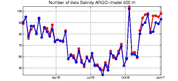
40 Figure 14: Time series of weekly RMS misfit of salinity ARGO-Model (Left) and number of observed profiles (right) at 8, 30, 150, 300 and 600 m (S-<X-Y>m-W-CLASS4 PROF-RMSD-MED-Jan2016-Dec2016) Page 40/ 60

41 The following panels in Figure 15 show the time series of salinity daily RMSs of the difference between model outputs and observations evaluated over the qualification testing period (2016): S-<X-Y>m-D- CLASS4-PROF-RMSD-MED-Jan2016-Dec The statistics are evaluated for nine different layers (0-10, 10-30, 30-60, , , , , , m). The differences between V4 and V3.2 systems are very small. The two systems present similar errors at all levels. The average value of RMS over the entire period is the one listed in Erreur! Source du renvoi introuvable.. The salinity error is generally higher above 150 m then the error decreases significantly below 150 m. Page 41/ 60

42 Page 42/ 60

43 Page 43/ 60

44 Figure 15: Time series of daily RMS of salinity at different vertical layers for V3.2 and V4 systems (S-<X-Y>m-D- CLASS4-PROF-RMSD-MED-Jan2016-Dec 2016) Table 13 summarizes the surface (3 m) salinity RMS differences and the Bias calculated comparing the analysis of product with the independent in-situ data (MB: coastal moored buoys) for the year In general, the two systems present similar skill and it has to be noticed that the number of available buoys is scarce in the qualification period. Variables/estimated accuracy: RMS diff Bias Depth Obs No. of Obs. S-SURF-D-CLASS2- MOOR-RMSD- Jan2016-Dec2016 S-SURF-D-CLASS2- MOOR-BIAS- Jan2016-Dec2016 SALINITY (psu) year 2016: V MB 8 SALINITY (psu) year 2016: V MB 8 Table 13: Salinity independent observation evaluation based on 1-year time series (2016) of analysis and Moored Buoys observations. Figure 16 shows an example of daily salinity time series of V3.2 (red line) and V4 (blue line) model outputs against Cabo de Gata coastal mooring (green line) for year The V3.2 and V4 modelling systems exhibit a good ability in representing the measurements and only little differences can be inferred by the two time series and in particular the two systems have similar RMS difference when comparing to the Cabo de Gata buoy. Page 44/ 60

45 Figure 16: Time series of daily surface salinity at Cabo de Gata buoy. Comparison between observations (green line), V3.2 model output (red line) and V4 model output (blue line). RMS and bias averaged over year 2016 are included in the plot (S-SURF-D-CLASS2-MOOR-RMSD-Jan2016-Dec2016, S-SURF-D-CLASS2-MOOR-BIAS-Jan2016- Dec2016). III.4 Sea Level Anomaly In Table 14 there are the RMS differences for the Sea Level Anomaly calculated comparing the analysis of product with each available satellite (along track observations) from January to December SEA LEVEL ANOMALIES (cm) RMS Diff Availability All Satellites /01/ /12/2016 ALTIKA 4 01/01/ /12/2016 CRYOSAT /01/ /12/2016 JASON 2/JASON 2N /01/ /09/2016 (Jason2) 3/11/ /12/2016 (Jason2N) JASON /09/ /12/2016 Table 14: Analysis evaluation based over 1 year time series (2016) for the Sea Level Anomaly for each available satellite. The following Figure 17 shows on the left panels the time series of weekly RMS of sea level anomaly misfits (observation minus model value transformed at the observation location and time before being assimilated), SLA-SURF-W-CLASS4-ALT-RMSD-MED-Jan2016-Dec2016, for the CMEMS Med-Currents Page 45/ 60

46 V3.2 system (red line) and the V4 system (blue line). On the right hand side the weekly time series of number of assimilated data is provided. The new system presents a better skill if compared to V3.2 system for each of the available satellite decreasing the RMS of about 0.4 cm in average. This improvement has been reached by changing the SLA assimilation scheme (as detailed in the description of the system), even if this change caused a reduction in the number of assimilated data (only in areas deeper than 1000 m) as can be noticed from the right panels of Figure 17. Page 46/ 60

47 Figure 17 Time series of weekly RMS of satellite-model misfit along SLA data track for all the satellites (top panel), Altika, Cryosat, Jason2/N and Jason3 (left) and corresponding number of assimilated data (right) (SLA- SURF-W-CLASS4-ALT-RMSD-MED-Jan2016-Dec2016) Figure 18 shows the time series of Sea Level Anomaly daily RMSs of the difference between model output and observations evaluated over the qualification testing period (2016): SLA-SURF-D-CLASS4- RMSD-MED-Jan2016-Dec Again the new system (blue line) presents better performances during all the simulated period if compared to V3.2 system (red line). Figure 18: Time series of daily RMS of Sea Level Anomaly for V3.2 and V4 systems (SLA-SURF-D-CLASS4-RMSD- MED-Jan2016-Dec 2016) Time series of daily basin averaged SLA compared to Satellite Delayed Time L4 AVISO dataset at 1/8 degree resolution is presented in Figure 19 for the year 2016 showing that the two numerical systems (V3.2 and V4) have almost the same pattern and are able to represent the temporal variability of the satellite data. In order to provide this comparison, the numerical SSH has been interpolated at 1/8 Page 47/ 60

48 degree resolution (same grid of the satellite data) and a yearly basin average SSH value (mean SSH) has been removed in order to obtain the numerical SLA. Figure 19: Time series of daily Sea Level Anomaly for V3.2 (red) and V4 (blue) systems compared to satellite delayed time L4 AVISO dataset at 1/8 degree resolution (green) III.5 Sea Surface Height Sea surface height quality is assessed by means of independent validation through coastal tide gauges. Table 15 summarizes the RMS differences and the Bias calculated comparing the analysis of product with the independent in-situ data (MB: coastal moored buoys) for the year The new system (V4) shows a slightly increased skill with lower Sea Level RMS with respect to the previous system (V3.2). Variables/estimated accuracy: RMS diff Bias Depth Obs No. of Obs. SL-SURF-D- CLASS2-TG-RMSD- Jan2016-Dec2016 SL-SURF-D-CLASS2- TG-BIAS-Jan2016- Dec2016 SSH (cm) year 2016: V MB 49 SSH (cm) year 2016: V MB 49 Table 15: Independent observation evaluation based on 1-year time series (2016) of analysis and Moored Buoys observations. Figure 20 shows an example of daily sea level time series of V3.2 (red line) and V4 (blue line) model outputs against Algeciras tide gauge next to the Gibraltar Strait (green line) for year The V3.2 and V4 modelling systems exhibit a good ability in representing the measurements and the V4 has a lower RMS with respect to the previous system. Page 48/ 60

49 Figure 20: Time series of daily sea level at Algeciras tide gauge. Comparison between observations (green line), V3.2 model output (red line) and V4 model output (blue line). RMS and bias averaged over year 2016 are included in the plot (SL-SURF-D-CLASS2-TG-RMSD-Jan2016-Dec2016, SL-SURF-D-CLASS2-TG-BIAS-Jan2016- Dec2016). III.6 Currents The predicted sea surface currents skill is assessed by means of independent validation through coastal moorings. Table 16 summarizes the RMS differences and the Bias calculated comparing the analysis of product with the independent in-situ data (MB: coastal moored buoys) for the year In general, the two systems present similar skills (better performance of the new system can be noticed when considering zonal currents) and it has to be noticed that the number of available buoys is scarce in the qualification period. Variables/estimated accuracy: RMS diff Bias Depth Obs UV-SURF-D- CLASS2-MOOR- RMSD-Jan2016- Dec2016 UV-SURF-D- CLASS2- MOOR-BIAS- Jan2016- Dec2016 Zonal Current (cm/s) year 2016: V MB 8 Zonal Current (cm/s) year 2016: V MB 8 Meridional Current (cm/s) year 2016: V MB 8 Meridional Current (cm/s) year 2016: V MB 8 No. of Obs. Table 16: Independent observation evaluation based on 1-year time series (2016) of analysis and Moored Buoys observations. Page 49/ 60

50 Figure 21 shows an example of daily zonal (left) and meridional (right) sea surface currents time series of V3.2 (red line) and V4 (blue line) model outputs against the Cabo de Palos coastal mooring (green line) for year The V3.2 and V4 modelling systems exhibit a quite good ability in representing the measurements and only small differences can be inferred by the two time series. Figure 21: Time series of daily sea surface currents at Cabo de Palos buoy. Comparison between observations (green line), V3.2 model output (red line) and V4 model output (blue line). Left: Zonal current 2016; right: Meridional current RMS and bias averaged over 1 year period are included in the plot (UV-SURF-D-CLASS2- MOOR-RMSD-Jan2016-Dec2016, UV-SURF-D-CLASS2-MOOR-BIAS-Jan2016-Dec2016). In addition to surface currents validation, an assessment of velocity derived variables is provided in terms of transport through the strait of Gibraltar. In Figure 22 the time series of the mean daily Net flux through the Gibraltar Strait is represented for Med-Currents V3.2 (red line) and V4 (blue line) systems. Page 50/ 60

51 Figure 22: Time series of daily mean Net Flux through the Gibraltar Strait for Mer-Currents V3.2 (red line) and V4 (blue line) systems. In Table 17 the comparison with literature fluxes (Soto-Navaro et al., 2010) is included showing that the new system (V4) fluxes are closer to the ones provided by literature with respect to the V3.2 system. Gibraltar Mean Flux [Sv] CMEMS V3.2 CMEMS V4 Soto-Navarro et al., 2010 Net ± Eastward ± 0.06 Westward ± 0.05 Table 17: Gibraltar mean fluxes [Sv] from Med-Currents V3.2 and V4 systems compared to literature values. Moreover a comparison of geostrophic currents has been performed for the year The geostrophic currents are evaluated using delayed time SLA satellites L4 data at 1/8 degree resolution and from model geostrophic currents interpolated on the same satellite resolution. U g = -g/f(dsla/dy) ; V g = g/f(dsla/dx) where U g and V g are the zonal and meridional geostrophic velocity anomaly; g is the gravity acceleration and f is the Coriolis parameter. Figure 23 shows 2016 winter (January-February-March) SLA maps and geostrophic currents (arrows) from satellite 1/8 degree resolution dataset and corresponding model outputs. The model is able to Page 51/ 60

52 represent the spatial pattern of the satellite SLA and geostrophic currents while it presents a positive bias. Figure 24 shows the same comparison, but for the summer period (July-August-September), showing the ability of the model to represent the satellite geostrophic currents. Figure 23: Maps of 2016 winter (Jan-Feb-Mar) geostrophic currents and SLA: satellite observations (top), V4 modelling system (bottom) Page 52/ 60

53 Figure 24: Maps of 2016 summer (Jul-Aug-Sep) geostrophic currents and SLA: satellite observations (top), V4 modelling system (bottom) III.7 Mixed Layer Depth In order to assess the model ability to reproduce the Mixed Layer Depth (MLD), monthly averaged 2D maps of MLD have been compared to a climatological datasets available from literature (Houpert et al., 2015) providing monthly gridded climatologies produced using MBT, XBT, Profiling floats, Gliders, and ship-based CTD data from different database and carried out in the Mediterranean Sea between 1969 and Figure 25 to Figure 28 show the 2D maps of climatological MLD from literature (top), monthly averaged MLD from MED-Currents V3.2 (bottom-left) and MED-Currents V4 system (bottomright). It can be noticed that during March 2016 (Figure 25), the modelled MLD in the Gulf of Lyon is shallower than the climatological value and slightly deeper in the Aegean Sea; during June 2016 (Figure 26) the modelled MLD is in general similar to the climatological one with a slightly deeper MLD in the North Adriatic Sea; during September 2016 (Figure 27) the Med-Currents V4 and V3.2 systems are very close to the climatology with a similar spatial pattern; in November 2016 (Figure 28) the 2 systems have similar performances with slightly deeper MLD in the Adriatic Sea and in the Aegean Sea South to Greece. In general it can be noticed that the numerical systems are able to represent the spatial and seasonal distribution of the MLD and the main differences can be due to the low resolution of the climatological dataset that moreover do not cover the whole domain of the Mediterranean Sea. Page 53/ 60

54 Figure 25: March MLD 2D maps. Top: climatological data from literature; left: March 2016 monthly averaged MLD from MED-Currents V3.2; right: March 2016 monthly averaged MLD from MED-Currents V4: MLD-D-CLASS1- CLIM-MEAN_M-MED Figure 26: June MLD 2D maps. Top: climatological data from literature; left: June 2016 monthly averaged MLD from MED-Currents V3.2; right: June 2016 monthly averaged MLD from MED-Currents V4: MLD-D-CLASS1-CLIM- MEAN_M-MED Page 54/ 60

55 Figure 27: September MLD 2D maps. Top: climatological data from literature; left: September 2016 monthly averaged MLD from MED-Currents V3.2; right: September 2016 monthly averaged MLD from MED-Currents V4: MLD-D-CLASS1-CLIM-MEAN_M-MED Figure 28: November MLD 2D maps. Top: climatological data from literature; left: November 2016 monthly averaged MLD from MED-Currents V3.2; right: November 2016 monthly averaged MLD from MED-Currents 4: MLD-D-CLASS1-CLIM-MEAN_M-MED Page 55/ 60